
Submitted:
09 November 2026
Posted:
11 November 2026
You are already at the latest version
Abstract
Financial stability may support investment and employment, yet environmental and social progress may respond differently. This study examines how bank capital adequacy, loan portfolio quality and financial market stress relate to renewable energy, per-capita greenhouse gas emissions and employment across European Union countries. Using unbalanced panels for 2010–2024 and 2015–2024, we estimate models with country and year fixed effects; common-sample comparisons and a composite sustain-ability index are exploratory. In the primary 26-country financial-stress panel, a 0.1-point higher stress index was associated with a 0.305 percentage-point smaller annual change in the employment rate. Still, the association was not statistically significant after adjustment for three outcomes. Environmental estimates and primary bank-capital estimates were uncertain, and inference methods disagreed for installed wind capacity. Exploratory models with outcome-specific controls retained a negative stress–employment association, although its statistical significance depended on the scope of multiple-testing adjustment. The composite index reflected this pattern mainly through employment. These findings highlight a recurring association between financial stress and employment and show why environmental and social outcomes should be assessed separately.
Keywords:
financial stability
; financial stress
; bank capitalisation
; sustainability
; renewable energy
; greenhouse gas emissions
; employment
; European Union
1. Introduction
Sustainable economic development requires sustained investment, firms able to adapt to economic change, and employment opportunities. The financial system supports these processes by financing firms and allocating resources across activities. Disruptions to financial intermediation can restrict access to credit, delay investment projects and increase the costs of adjustment. The European Central Bank defines financial stability as the system's ability to withstand shocks and avoid major disruptions to financial intermediation and real economic activity [1]. This resilience matters for a sustainable economy, but its environmental and social contribution also depends on the activities that finance supports.
Financial resilience and the contribution of finance to sustainability address different questions. Well-capitalised banks may continue to finance high-emission activities, while calm financial markets do not necessarily support investment in renewable energy. At the same time, the transition to a lower-carbon economy requires investment in new infrastructure and technologies and may alter firms' risk profiles and financing needs. As Campiglio explains, credit market imperfections and lending decisions can constrain low-carbon investment even when carbon pricing provides an incentive to invest [2]. Whether financial conditions support sustainability therefore depends both on the continuity of financing and on where financial resources are directed.
European Union policy brings these questions together. The European Commission's strategy for financing the transition to a sustainable economy emphasises economic transformation, inclusiveness and financial resilience [3]. Pursuing these objectives together does not guarantee equally favourable outcomes across all dimensions. Sustainable finance concerns the allocation of resources towards environmental and social objectives, whereas financial stability concerns the system's ability to function under adverse conditions [4]. Examining environmental and social outcomes separately helps establish how these related policy aims align in practice.
Previous studies do not show a uniform relationship between financial stability and sustainability. In EU countries, Şahin and Arzova [5] report different associations with green growth for banking stability and access to credit. Ozili and Iorember [6] find that associations vary across sustainability indicators and economic contexts. Hoang [7] reports heterogeneous links between financial stress and environmental outcomes, while Javed et al. [8] examine how macro-financial stability shapes the finance–green-growth relationship in developing economies. These studies use different financial measures, samples and outcomes, making it difficult to generalise their findings to environmental and social changes in the EU. Together, these studies raise a more specific question for the EU: do distinct aspects of financial stability accompany similar changes in environmental and social outcomes?
Three issues motivate that question. First, the stability indices and risk measures used in the previous studies capture different financial conditions. Their results leave open the question of whether bank capital adequacy, loan portfolio quality, and market stress have similar relationships with sustainability. Second, studies centred on green growth or environmental indicators give less insight into whether environmental improvements coincide with social progress. Third, the choice of environmental measure matters: a higher share of renewable energy, more generating capacity, and lower emissions describe different aspects of the transition. Examining these issues within an EU framework can reveal which relationships recur across measures and which are specific to a particular outcome.
This study aims to assess the associations between different dimensions of financial stability and changes in environmental and social sustainability indicators across European Union countries. Financial stability is examined through three measures: the Tier 1 capital ratio, the non-performing loan ratio, and the Country-Level Index of Financial Stress (CLIFS). CLIFS and Tier 1 define the two primary analyses; the non-performing loan ratio is examined in a separate banking comparison and exploratory common-sample models. Environmental sustainability is assessed using renewable energy expansion and changes in per-capita greenhouse gas emissions. At the same time, the social dimension is represented by changes in the employment rate among people aged 20–64. A supplementary composite sustainability index covering environmental, social, and economic dimensions is also examined. This approach enables assessment not only of the associations between individual financial stability measures and selected sustainability outcomes, but also of whether these associations are consistent across sustainability dimensions.
The study uses two unbalanced EU panels: a financial market-stress panel for 2010–2024 and a bank-capitalisation panel for 2015–2024. Models with country and year fixed effects relate financial conditions to annual outcome changes. Subsequent exploratory analyses compare financial measures on common country-years, add controls relevant to each outcome, and examine a composite sustainability index and nonlinear relationships. Section 3 explains the samples, timing and measures; the appendices provide the technical details.
The study provides evidence on how distinct aspects of financial stability relate to environmental outcomes and employment. It examines capital adequacy, loan quality and market stress separately, and places environmental outcomes alongside employment. The common-sample comparisons show how the findings change with outcome-specific controls, while the supporting index reveals which components account for an aggregate association. This approach makes it possible to assess how far a broad claim about financial stability and sustainability is supported by the individual relationships.
Higher financial market stress is associated with smaller annual increases in the employment rate in the primary and exploratory common-sample analyses. However, the primary association is not statistically significant after adjustment for the three outcomes, and the exploratory result depends on how many tests are included in the adjustment. The environmental estimates do not establish a consistent favourable association with lower stress or higher bank capitalisation. The composite index result largely reflects its employment component. Overall, the evidence is more specific to employment than to sustainability outcomes as a whole.
The remainder of the article reviews the theoretical and empirical literature, describes the data and methods, presents the results, discusses their research and policy implications, and concludes.
2. Financial Stability and Sustainability: Mechanisms and Evidence
2.1. Financing Continuity and Low-Carbon Investment
Financing continuity provides one reason to expect a relationship between financial stability and sustainability. Renewable energy infrastructure and production changes often require large initial investments, with returns and financial obligations extending over many years. Disruptions to credit can delay these projects or threaten their completion. Resilient intermediaries may be better able to absorb losses and maintain lending when economic conditions deteriorate. The environmental contribution, however, depends on financing projects that reduce emissions, expand renewable energy, or introduce cleaner technologies. Campiglio (2016) explains how credit market imperfections, lending decisions and project risk–return characteristics can constrain low-carbon investment, and discusses the potential role of monetary and macroprudential policies in addressing these barriers [2].
The relationship between financial system conditions and environmental sustainability is not straightforward, as access to finance does not necessarily ensure that investment is directed towards environmentally sustainable activities. Mensah and Näsström (2022), using a broad international sample, examine the relationship between banking sector performance and renewable energy consumption and find that the results differ across country groups [9]. Beka and Abazi-Alili (2024), analysing 38 OECD countries and five Western Balkan countries over 2010–2022, similarly identify differences in the associations between banking sector performance indicators and renewable energy consumption across the two country groups [10]. OECD countries report a statistically significant positive association between financial stability, measured by the banking system Z-score, and renewable energy consumption. In the Western Balkan countries, the association with the Z-score was negative but not statistically significant at the 5% level. In contrast, a statistically significant positive association was reported for the non-performing loan ratio, which the authors use as an asset-quality indicator. Since a higher non-performing loan ratio indicates poorer loan portfolio quality, this result should not be interpreted as evidence that improvements in asset quality are positively associated with renewable energy consumption. Overall, these findings suggest that the relationships between banking sector conditions and environmental outcomes may vary across economic and financial environments.
Renewable energy consumption captures one part of this relationship. Financial systems can finance clean energy while also supporting activities that raise total energy demand and emissions. Examining renewable energy expansion alongside greenhouse gas emissions, therefore, provides a fuller view of the environmental changes associated with financial conditions.
Financial resilience and access to investment finance can also move differently. A higher capital adequacy ratio may result from more regulatory capital, fewer risk-weighted assets, or both. Banks can therefore improve the ratio while restricting lending. Better loan quality may strengthen their capacity to finance new projects, but the destination of that finance remains a separate question. Capital and loan-quality ratios describe resilience and credit risk; they do not directly measure lending to environmentally sustainable activities.
The distinction between financial stability and access to finance is also illustrated by Şahin and Arzova (2026), who examined the relationships between political, macroeconomic, and financial stability and green economic growth using data from 27 EU countries over 2012–2021 [5]. Their findings indicate that the association between banking stability, measured by the Z-score, and green economic growth was not statistically significant in the full sample. Domestic credit to the private sector showed a positive association, but was statistically significant only at the 10% level. Additional subgroup analyses revealed a weak positive association between credit provision and green economic growth in the more economically developed EU countries. In contrast, the corresponding association was not statistically significant in Central and Eastern European countries. These findings suggest that financial system resilience and access to finance may exhibit different relationships with environmental outcomes and that these relationships may vary with countries’ economic and institutional characteristics. This provides a rationale for separately examining the associations between various financial stability indicators and selected environmental sustainability outcomes, including renewable energy expansion and per-person greenhouse gas emissions.
2.2. Capitalisation, Asset Quality and Financial Market Stress
Assessing the relationship between financial stability and sustainability requires consideration of different aspects of financial system conditions, as bank capital adequacy, asset quality, and financial market stress reflect distinct mechanisms of financial resilience and risk. The Tier 1 capital ratio, defined as Tier 1 capital relative to risk-weighted assets, indicates banks’ capacity to absorb potential losses. The non-performing loan (NPL) ratio reflects the quality of the loan portfolio and the level of credit risk. Meanwhile, the Country-Level Index of Financial Stress (CLIFS) captures financial market stress associated with asset price fluctuations, increased uncertainty, and co-movements across financial market segments. Duprey et al. (2017) developed a methodology for identifying episodes of systemic financial stress. They demonstrated that periods of elevated financial market stress may be associated with substantial declines in real economic activity. They also found that, in most identified systemic stress episodes, financial market stress preceded real economic stress [11]. These findings support the relevance of financial market stress measures when examining the relationship between financial stability and economic and sustainability outcomes.
These financial dimensions suggest different pathways to sustainability outcomes. Capital adequacy and better loan quality may help banks sustain lending through difficult periods. Market stress may accompany tighter financing conditions, postponed investment and more cautious hiring, affecting both renewable projects and employment. At the same time, an economic slowdown can reduce energy consumption and emissions. The same deterioration in financial conditions could therefore coincide with weaker employment and lower emissions, making separate outcome comparisons essential.
The complexity of the relationship between financial stability and sustainability is further illustrated by Ozili and Iorember (2024), who analysed data from 26 countries over 2011–2018 using the system generalised method of moments (system GMM) [6]. They found that the relationship between financial stability and sustainable development depends on the sustainability measure employed and countries’ economic characteristics. Their analysis of a composite sustainable development index identified a statistically significant association with financial stability, with a negative relationship reported for Asian countries. Analyses of individual Sustainable Development Goals (SDGs) also revealed heterogeneous findings. Notably, financial stability was positively associated with SDG 3 (Good Health and Well-Being) and SDG 7 (Affordable and Clean Energy) in countries with higher banking-sector capital buffers. These findings suggest that bank capital buffers may condition the relationship between financial stability and specific dimensions of sustainable development, and that the nature of the association depends on the sustainability outcome considered.
The role of financial stability in green economic growth was further investigated by Javed et al. (2026), who examined 34 developing economies from 1991 to 2022 [8]. Their study used a financial risk rating covering external financial vulnerabilities to examine whether macro-financial stability conditions the relationship between financial development and environmental outcomes. The authors reported that greater macro-financial stability strengthened the positive associations between financial institution and financial market development and green economic growth. Their interaction analyses also indicated more favourable associations with renewable energy consumption and lower carbon dioxide emissions intensity. These findings suggest that financial stability may be relevant not only as an independent characteristic of the financial system but also as a condition shaping the relationship between financial development and environmental outcomes.
The complexity of the relationship between financial market stress and environmental sustainability is also highlighted by Hoang (2026), who analysed 36 countries over 1991–2023 using panel quantile regression [7]. The results indicate that the associations between financial stress, renewable energy consumption, and carbon dioxide emissions vary across conditional quantiles of the outcome distributions. Both positive and negative associations were identified, suggesting that increases in financial stress are not uniformly associated with improved or deteriorating environmental outcomes. The study also reports adverse associations between geopolitical risk and the energy transition and environmental conditions. These findings complement previous research by indicating that the relationships between financial instability and environmental outcomes may depend on economic conditions and the characteristics of the indicators examined.
The literature thus provides reasons to distinguish between financial measures and outcomes. Bank capital ratios, loan quality, composite stability measures and macro-financial risk ratings describe different conditions. Studying capital adequacy, asset quality and market stress separately in EU countries allows us to compare their relationships with selected environmental and social changes without assuming that they represent equivalent improvements in stability.
2.3. Renewable Energy, Emissions and Employment
Improvements in environmental outcomes do not necessarily coincide with improvements in social outcomes. Renewable energy can expand through new infrastructure, technological improvements and public support. Emissions can decline because production becomes cleaner, energy use becomes more efficient, or economic activity contracts. Employment encompasses participation in economic activity and access to labour market opportunities. During periods of financial stress, a slowdown may therefore lead to both lower emissions and weaker employment. Assessing those outcomes separately distinguishes a cleaner economy from an economy that emits less because it produces less.
Renewable energy development can also be assessed using different indicators that capture distinct aspects of the energy transition. Tu et al. (2022), examining the determinants of renewable energy development in EU countries, highlight the importance of economic, technological, and institutional factors [12]. Valdés Lucas et al. (2016), investigating the relationship between renewable energy deployment and energy security in the EU, emphasise their interdependence and the relevance of energy system structure and reliance on external energy resources [13]. These studies suggest that renewable energy development depends on a range of economic and structural conditions, which may lead to heterogeneous associations with financial stability indicators. Moreover, an increase in the renewable share of energy consumption does not necessarily imply a proportional expansion of new generation capacity, as the change in the share also depends on total energy consumption. By contrast, the net change in installed wind capacity directly captures the expansion or contraction of physical generation capacity. Still, it does not measure actual electricity generation or the monetary value of investment. These indicators therefore provide complementary rather than equivalent information about the energy transition.
The STIRPAT framework developed by York et al. (2003) provides a theoretical basis for analysing changes in GHG emissions by relating environmental impacts to population, affluence, and technology [14]. This perspective helps explain why emissions are influenced not only by the energy transition but also by the scale of economic activity and production technologies. The European Environment Agency identifies several interrelated drivers of declining GHG emissions in the EU, including lower energy-production carbon intensity, improvements in energy efficiency, changes in the structure of economic activity, and climate policy measures [15]. At the same time, expanding economic activity may increase energy demand and emissions, making the relationship between financial stability and GHG emissions ambiguous. A financial system capable of supporting investment may facilitate the adoption of less carbon-intensive technologies while also financing broader economic expansion. Because these mechanisms may operate in opposing directions, the relationship between financial stability and changes in GHG emissions remains an empirical question.
Within the social dimension of sustainability, the employment rate captures an important aspect of economic participation. However, changes in employment depend not only on financing conditions but also on the business cycle, workforce qualifications, and demographic structure. Consolo et al. (2026), examining labour force developments in the euro area, highlight the roles of population ageing, educational attainment, and migration in shaping labour supply and labour force participation [16]. An, Bluedorn, and Ciminelli (2021), investigating Okun’s law across economies and worker groups, demonstrate that the cyclical sensitivity of unemployment varies with economic development and demographic characteristics [17]. Although these studies focus on labour force participation and unemployment rather than the employment rate used in the present study, they provide a basis for considering how economic and structural conditions may shape the relationship between financial market stress and employment. Increasing financial stress may restrict firms’ ability to finance operations and investment, encourage more cautious hiring decisions, and consequently be associated with weaker employment outcomes. However, the strength of these associations may vary according to labour market structure and broader economic conditions.
These differences form the basis for the empirical comparison. Renewable expansion, emissions and employment each require measures and controls suited to the outcome being studied. An index combining environmental, social and economic indicators can then summarise their joint movement. Reading that index alongside its components shows whether an aggregate association reflects broad progress or is concentrated in one dimension.
3. Data and Empirical Approach
3.1. Country Panels and Measures
The unit of observation is a country in an outcome year. The primary financial market-stress panel contains 371 country-year observations from 26 current EU members over 2010–2024. The primary bank-capitalisation panel contains 258 observations covering the current EU27 over 2015–2024. Estonia is excluded from analyses requiring CLIFS, including the stress and common-sample analyses, but remains in the primary capital analysis. Data availability and the exclusion of employment changes crossing reported statistical breaks produce unbalanced panels. The country group follows current EU membership; some countries were not members throughout the study period. Appendix A explains sample construction.
Financial stress is measured using the average monthly CLIFS value from the year preceding the outcome year. The annual average is calculated only when all 12 monthly observations are available. The Tier 1 and non-performing loan ratios use the preceding year-end observation from ECB consolidated banking data. A higher Tier 1 capital ratio indicates stronger bank capital adequacy, whereas higher NPL and CLIFS values indicate poorer asset quality and greater financial market stress, respectively. A five-percentage-point increase is the reported contrast for each banking ratio; a 0.1-index-unit increase is the contrast for CLIFS. These scales support readable interpretation within each measure. They are not a claim that the contrasts represent equivalent changes in risk. Table 1 summarises the financial measures, their interpretation and the corresponding study coverage.
The primary financial market-stress analysis examines annual changes in the share of renewable energy in gross final energy consumption, territorial greenhouse gas emissions per capita, and the employment rate among individuals aged 20–64. Renewable and employment changes are measured in percentage points. Changes in greenhouse gas emissions are measured in tonnes of CO₂ equivalent per capita, excluding emissions and removals from land use, land-use change and forestry (LULUCF), as well as separately reported emissions from international aviation, maritime transport and other memorandum items. The primary Tier 1 analysis uses annual net changes in installed wind power capacity, logarithmic changes in greenhouse gas emissions, and the same change in the employment rate. The wind outcome is the change in capacity between 31 December of consecutive years, divided by the population on 1 January of the outcome year, in millions. Its unit is megawatts per million residents. Emissions log changes are 100 times the logarithm of the ratio between successive years, expressed as log-per cent points.
The environmental measures provide complementary views of the transition. The stress analysis examines changes in the energy mix and absolute changes in per-person emissions. The capital analysis examines net additions in wind capacity and proportional changes in emissions. A decline in wind capacity is retained because it can reflect retirements or statistical revisions; it is a net stock change, not negative investment expenditure. All employment models use the rate among people aged 20–64. Appendix A documents the source series, flags and reporting parameters.
The sample rules preserve the distinction between economic changes and reporting changes. Employment changes crossing a reported break are excluded, while observations with remaining definition differences receive a separate sensitivity check. Missing financial observations are not replaced by zero, and missing controls are not interpolated. Differences between the primary panels therefore reflect both outcome definitions and available observations. The common-sample extension holds the observations fixed when comparing specifications within each outcome.
3.2. Within-Country Comparisons and Timing
The linear models compare annual changes within countries. Country fixed effects account for each country's typical annual-change pattern over the observed period; year fixed effects account for shifts shared across countries. The original controls are log real GDP per person, adjusted for purchasing power, and consumer-price inflation, both measured two years before the outcome. Each country-year receives equal weight. The comparison asks whether different levels of financial stress, bank capitalisation, and loan quality are associated with different annual changes in outcomes within countries.
The timing of financial stress is central to that interpretation. An annual outcome change compares two successive years, with the first year also being the CLIFS averaging period. Stress, therefore, precedes the endpoint but overlaps with the baseline of the change. The estimated relationship may reflect financial and economic conditions already developing together in that baseline year. Stricter timing checks move the financial exposure before the baseline and the controls earlier still, testing whether the pattern also appears with greater temporal separation. These lag choices help interpret the association, though the observational design remains vulnerable to confounding and feedback.
The uncertainty procedures allow observations from the same country to be related over time. In the capital models, a small-sample adjustment also accounts for the limited independent country-level information informing the estimate [18, 19]. This adjusts the standard errors, confidence intervals and tests, rather than the observed data or coefficient estimates. Within each primary analysis, Holm's adjustment considers the three outcome tests together. A separate bootstrap calculation checks how the results depend on the uncertainty procedure. This comparison matters particularly for capitalisation, where much of the informative variation comes from a few countries. Appendix B gives the covariance methods, degrees of freedom, interval definitions and groups of tests used in each adjustment.
3.3. Exploratory Comparisons and Aggregation
We distinguish the two primary analyses from later exploratory comparisons. The market-stress analysis plan was fixed locally before its estimation. The bank-capital analysis was developed after the market-stress results were known, and the tailored-control models, composite index and nonlinear analyses followed both primary analyses. This sequence explains which questions guided each analysis and which arose from the preceding findings; it does not constitute external preregistration.
The subsequent comparisons use common recent country-years for all three financial measures and incorporate additional controls selected to reflect economic and structural factors relevant to each outcome. The wind capacity specifications also account for economic growth, energy import dependence, and existing installed wind capacity. The emissions specifications include economic growth, manufacturing share and energy intensity, while the employment specifications control for economic growth, tertiary educational attainment and the share of older individuals in the working-age population. These controls are dated two years before the outcome. The matched original-control models use the same country-years as their tailored counterparts, allowing a clearer comparison of specifications. Appendix D explains the controls and retained source sensitivities.
The models examining changes in installed wind power capacity and employment rates are each estimated using 246 country-year observations covering 26 countries. The emissions specifications use 238 country-year observations across 25 countries because eight Bulgarian manufacturing observations are unavailable and are not imputed. The nine financial coefficients from the tailored-control models are treated as a single family of tests for multiple-testing adjustment. A broader multiple-testing adjustment covers 57 designated exploratory tests, including financial coefficients from additional model specifications and tests of nonlinear relations. Reporting both adjustments makes clear how conclusions change when a broader set of hypotheses is considered. Differences between coefficients are descriptive unless a direct statistical contrast is provided. Neither the common sample nor its tailored controls displace the original primary results.
Finally, a supporting index combines the renewable energy share, favourably oriented emissions per person, employment, and real income per person. It follows the principle that normalisation, weighting and sensitivity should be transparent [20]. Each component is standardised against the fixed EU27 distribution in 2014. The environmental, social, and economic pillars receive equal weight, with the two environmental components each accounting for half of the pillar's weight. The main index regressions use 246 eligible country-year observations. Annual-change and level models form an exploratory family of six tests, with a broader adjustment reported as well. Appendix E provides construction and alternatives; Appendix F reports the nonlinear comparisons. These exploratory comparisons supplement the primary results.
4. Results
4.1. Financial Market Stress and Employment Progress
Higher financial market stress accompanies weaker annual employment improvement in the primary EU26 panel. A 0.1-point higher prior-year CLIFS is associated with a 0.305-percentage-point smaller change in the employment rate among people aged 20–64. This means a smaller increase, or a larger decline, in the share employed. The marginal 95% interval runs from −0.574 to −0.037 percentage points. After considering the three outcomes together, however, the Holm-adjusted p-value is 0.083; the separately adjusted bootstrap p-value is 0.206. Neither procedure rejects the null hypothesis at the 5% level.
Figure 1 places this employment pattern beside the environmental results from both primary analyses. The point estimates suggest that financial conditions carry different information about labour-market adjustment and environmental progress. The environmental intervals allow associations in either direction, while the negative stress–employment estimate remains uncertain after the three-outcome adjustment.
The negative employment estimate is not driven by a single country. Removing each country in turn leaves all 26 coefficients negative, ranging from approximately −0.343 to −0.183 percentage points. The direction thus persists across samples with different combinations of national banking systems and labour markets.
The timing check gives a different picture. When stress is measured before the baseline year of the employment change, the estimate is positive and imprecise: 0.0666 percentage points per 0.1-point increase in CLIFS (95% CI: −0.3021 to 0.4353; p = 0.713). A model containing both stress lags gives a negative but imprecise sum of −0.1229 percentage points (95% CI: −0.5319 to 0.2862; p = 0.542). The recurring negative pattern therefore concerns stress during the baseline year and the annual change that follows, when financial and labour-market conditions may already be evolving together. Appendix C reports the timing and country-deletion checks.
4.2. Environmental Progress and Bank Capitalisation
The environmental estimates allow for both favourable and unfavourable relationships. In the primary financial market-stress analysis, a 0.1-unit increase in CLIFS is associated with a 0.060-percentage-point decrease in the renewable energy share (95% interval: −0.307 to 0.188). The emissions estimate is 0.027 tonnes of CO₂ equivalent per person, with an interval from −0.065 to 0.118. Both point estimates suggest less favourable environmental changes under greater stress, but each Holm-adjusted p-value is 1.000. These estimates do not establish an environmental advantage associated with lower stress.
The bank-capitalisation analysis also produces mixed results, with no clear pattern emerging across the outcomes. A five-percentage-point higher Tier 1 ratio is associated with 15.66 MW less in annual net wind capacity expansion per million residents. Its primary 95% interval extends from 37.72 MW less to 6.41 MW more, with a three-test adjusted p-value of 0.354. The negative point estimate is substantively different from the expected financing-continuity benefit, but the primary uncertainty does not establish that higher capitalisation reduces wind expansion. For emissions, the coefficient is −1.061 log-per cent points, with an interval from −3.250 to 1.128. Employment is near zero at −0.031 percentage points, with an interval from −0.449 to 0.388.
For wind capacity, statistical support depends on the uncertainty method. The primary capital test does not reject at the 5% level, whereas the separately adjusted restricted wild-cluster bootstrap gives a p-value of 0.041. Both assess the same negative coefficient; the disagreement concerns its statistical significance. We use the primary analysis for the main conclusion and report the bootstrap result as evidence of sensitivity to the inference method. Figure 1 shows the primary intervals; Appendix C provides both sets of adjusted tests.
The distribution of capital variation helps explain this sensitivity. Estonia accounts for almost half of the Tier 1 variation remaining after other model factors are accounted for. Although the panel covers 27 countries, much of the information about the capital relationship comes from a single national experience. The primary uncertainty procedure accounts for that concentration and produces a wide wind interval. Appendix C reports the concentration and degrees-of-freedom measures.
Taken together, the environmental results show why the measures need to remain distinct. Renewable shares describe the energy mix, wind capacity records physical expansion, and emissions reflect both production and technology. Figure 1 uses a separate scale for each outcome. The clearer recurring pattern concerns employment, while understanding the environmental relationships will require data linking financing conditions more closely to the type and timing of transition activity.
4.3. Comparing Financial Dimensions with Outcome-Specific Controls
In the common recent sample, financial market stress continues to accompany weaker employment improvement, while capitalisation and asset quality do not exhibit a generally favourable relationship across outcomes. The tailored employment estimate is −0.226 percentage points per 0.1-point increase in CLIFS, with a marginal 95% interval from −0.347 to −0.105. Its adjusted p-value is 0.015 across the nine tailored coefficients, but 0.093 across the broader set of 57 designated tests. The exploratory estimate has the same negative sign as the primary estimate, although differences in samples, controls and testing groups prevent a direct comparison of statistical support. Its adjusted statistical significance also depends on which hypotheses are included in the multiple-testing adjustment.
Figure 2 compares original and tailored controls on identical country-years within each outcome. Holding the sample fixed shows how the estimates change when economic demand and outcome-specific circumstances are included in the comparison. For employment, the additional factors are growth, educational attainment, and the age composition of the working-age population. The estimated association between financial market stress and annual changes in the employment rate remains negative after accounting for the additional control variables. The analysis of installed wind power capacity also considers existing installed capacity and energy import dependency, while the greenhouse gas emissions analysis accounts for manufacturing share and energy intensity. These additional controls help interpret the results in the context of relevant economic and energy-sector characteristics, while recognising that the outcomes measure different aspects of sustainability.
Capitalisation and non-performing loans show no common favourable pattern across wind, emissions and employment. The signs and uncertainty differ by outcome. Their interpretation also differs: a higher Tier 1 ratio indicates more capital relative to risk exposure, whereas a higher NPL ratio indicates poorer loan quality. The separate estimates identify the stress–employment pattern as a specific relationship, rather than a result shared by all financial measures.
The employment direction persists after additional country deletions in the tailored model: all 26 omitted-country coefficients are negative, ranging from approximately −0.245 to −0.195 percentage points. A sensitivity analysis excluding flagged education and age-composition controls retains a negative estimate of about −0.286, but uses only 180 country-years and has a nominal p-value near 0.040. The smaller sample is a material part of that comparison. Source flags deserve attention, yet deleting flagged observations changes both the information and the coverage; it cannot be interpreted as a purely measurement correction applied to an otherwise identical panel. Appendix D reports the matched comparisons and relevant source sensitivities.
The exploratory comparisons add a specific finding to the primary analysis: the negative stress–employment pattern recurs after accounting for growth, education and age composition. Financial market stress is the measure most consistently linked to weaker employment progress in these models. The environmental and bank-ratio evidence remains less settled. The smaller emissions sample excludes Bulgaria, and changes in national policies, investment conditions, and other unmeasured factors may still shape the observed relationships.
4.4. What an Aggregate Sustainability Measure Adds
The supporting annual sustainability index reproduces the negative association with financial market stress mainly through employment. A 0.1 higher CLIFS is associated with a −0.0225-point annual index change, with a marginal 95% interval from −0.0356 to −0.0093. The six-test adjusted p-value is 0.019; the broader 57-test adjustment gives 0.176. Statistical support is weaker when all 57 exploratory questions are considered together. Within the focused index comparison, it gives a coherent summary of slower progress under greater financial market stress. The score uses fixed component standardisation and weights, so its units are weighted component score points rather than percentages or an official sustainable-development rating.
Figure 3 shows the annual index estimates alongside the point decomposition of financial market stress. The employment-based social pillar supplies approximately 57.3% of the negative CLIFS coefficient. A negative index association can be driven by weaker employment progress even if environmental relationships remain uncertain. Aggregation thus makes the outcome pattern easier to summarise while also illustrating how a broad label can hide its principal component.
The negative financial market stress sign persists across all 36 pillar-weight combinations and under income exclusion. Its nominal p-value nevertheless rises to approximately 0.159 in the weight comparisons. The sign is therefore less sensitive to these choices than the degree of precision. Capitalisation is more sample-sensitive: its annual-index coefficient is positive on its own 258 available country-years and negative on the 246 matched country-years, with neither estimate precise. No level result passes the six-test adjustment. Appendix E records these comparisons. The nonlinear checks in Appendix F provide no adjusted evidence for the specified curvature or threshold. Their small, inconsistent improvements when predicting omitted country-year observations do not change the substantive interpretation of the linear results.
5. Discussion
The EU evidence points to different relationships across financial and sustainability dimensions. The recurring negative stress–employment pattern stands out relative to the environmental and banking-ratio estimates. The two primary analyses cover different periods, samples and environmental measures, while loan quality enters chiefly through secondary and exploratory analyses. The contribution is therefore a comparison of specific relationships, with common-sample extensions helping to distinguish changes in specification from changes in coverage.
The most persistent directional pattern concerns financial market stress and employment. In the original panel, a 0.1-unit increase in CLIFS was associated with a 0.305-percentage-point smaller annual change in the employment rate. Although the marginal confidence interval excluded zero, neither the three-outcome Holm adjustment (p = 0.083) nor the separate bootstrap adjustment (p = 0.206) rejected at the 5% level. The exploratory estimate with employment-specific controls was also negative (−0.226 percentage points), passing the nine-test adjustment (p = 0.015) but not the broader 57-test adjustment (p = 0.093). When financial market stress was measured before the baseline year for the employment change, the estimate was positive and imprecise. Thus, the repeated negative estimates concern models in which measured stress overlaps the baseline year; they do not demonstrate a delayed employment response or show that reducing stress would increase employment.
The environmental findings provide no consistent evidence of a favourable association with greater financial stability. Estimates of renewable share and per-person emissions in the primary stress analysis were imprecise. In the primary capital analysis, a 5-percentage-point higher Tier 1 ratio was associated with 15.66 MW less in annual net wind capacity change per million residents. The primary adjusted test did not reject the null hypothesis (p = 0.354), whereas the separate bootstrap test did (p = 0.041); statistical support for the negative estimate therefore depends on the inference procedure. The capital–emissions estimate was also imprecise, and the exploratory NPL estimates did not show a consistent favourable pattern across wind, emissions, and employment. These findings leave open the possibility of relationships that this study cannot estimate precisely. They also caution against comparing the two primary analyses as direct replications: renewable share differs from physical wind capacity, and absolute changes in emissions differ from logarithmic changes.
Financing continuity offers a plausible interpretation to investigate. Resilient banks may sustain lending through difficult periods, but a higher Tier 1 ratio can also reflect a reduction in risk-weighted assets. These country-level models do not observe the lending decisions needed to distinguish those pathways. Şahin and Arzova similarly find different green-growth associations for banking stability and domestic credit [5], while Ozili and Iorember report relationships that vary with the sustainability outcome and conditioning factors [6]. Together, these findings support the study of financial resilience and the allocation of finance as related but distinct questions.
Differences from earlier environmental studies also reflect what each study measures. Hoang reports associations between financial stress and environmental outcomes that vary across countries and conditional quantiles of environmental outcomes [7]. Javed and colleagues examine whether a macro-financial risk rating conditions the relationship between financial development and green growth in developing economies [8]. The present study adds employment to the EU comparison and distinguishes market stress from bank capital and loan quality. Across these settings, the choice of financial measure and sustainability outcome is central to the interpretation.
The supporting index illustrates both the value and the limits of aggregation. Its negative annual-change association with CLIFS passes the six-test adjustment but not the broader 57-test adjustment. Employment accounts for approximately 57.3% of the weighted point estimate in the index decomposition. That share has no reported confidence interval and is neither a causal contribution nor a proportion of explained variation. Fixed reference values and explicit weights make the construction transparent, as recommended for composite indicators [20], but the index permits improvement in one component to offset deterioration in another. It also omits aspects such as job quality, distribution, and environmental conditions beyond the selected energy and emissions measures. The exploratory nonlinear tests found no adjusted evidence for the specified curvature or fixed-median threshold; this does not rule out other nonlinear relationships.
The fixed-effects design describes conditional within-country relationships. Changing national conditions may affect both finance and sustainability, and the timing results show why baseline-year stress requires particular care. Country-clustered inference accounts for dependence within countries but still relies on assumptions about dependence across them [18]. Concentrated capital variation and differences in reporting perimeters further affect precision and comparability. These features guide the next research step: combining identified financial disturbances with project, firm or lending data to examine how financing continuity connects financial resilience to investment and employment. The present evidence identifies a recurring stress–employment pattern and an environmental relationship that remains uncertain.
6. Policy Implications
Financial and sustainability monitoring benefit from keeping capital adequacy, loan quality and market stress visible as separate indicators. The recurring negative stress–employment estimates make the CLIFS measure relevant to discussions of social adjustment alongside labour-market information. The primary estimate does not reach statistical significance after the three-outcome adjustment, and the earlier-stress check changes its direction. CLIFS is therefore a contextual indicator in this study, rather than a validated employment predictor or intervention trigger. Decisions about capital requirements need evidence on their own effects; these associations do not establish such effects.
Sustainability reporting should preserve the component outcomes behind an aggregate score. In this study, employment accounts for most of the negative CLIFS point estimate in the supporting index; the index does not establish a general environmental association. Reporting employment, renewable energy share, net wind capacity, and emissions separately would show which outcome drives the aggregate result. Renewable share and wind capacity should also retain their distinct definitions, since a change in the energy mix does not necessarily indicate an equivalent change in generating capacity. The index can summarise a stated set of measures, but should not substitute for them in assessing policy progress.
For investment and labour policy, the findings help identify where more direct evidence would be most useful. Project and lending records could reveal whether financing interruptions delay transition investment and which projects are affected. Linked firm and worker data could show whether employment adjustment comes through hiring, job losses or changes in participation. Evaluating policies using those data would link financial conditions to decisions that aggregate country indicators cannot capture.
7. Conclusions
Does financial system stability foster sustainability? In these EU country panels, the answer depends on the financial dimension, the outcome, and the strength of the required inference. In the primary financial market-stress analysis and the exploratory common-sample models, higher financial market stress is associated with smaller annual changes in the employment rate. However, the primary association is not statistically significant after adjustment for the three outcomes, and measuring stress before the baseline year gives a positive but imprecise estimate. The environmental estimates and primary Tier 1 results do not establish a consistent favourable relationship with the outcomes studied. For wind capacity, the primary and bootstrap tests reach different conclusions about statistical significance. Overall, the evidence points to a recurring stress–employment pattern, while a broader environmental benefit from greater financial stability remains unestablished.
The study contributes by bringing capitalisation, asset quality and market stress into a differentiated account of environmental and social change. A supporting sustainability index reproduces the stress pattern largely through employment, thereby showing why an aggregate association should be interpreted with caution. The common-sample comparisons add evidence under outcome-specific controls, yet remain exploratory and sensitive to broader adjustment. Taken together, the results highlight a recurring stress–employment pattern, while the environmental associations and the evidence for Tier 1 capitalisation and loan quality remain less conclusive.
This distinction matters for assessing progress. A financial indicator may accompany changes in employment without showing a clear relationship with environmental outcomes. Reporting the components makes that pattern visible and keeps the interpretation of an aggregate sustainability score tied to what actually changes.
Further research can address this boundary in three focused ways. Designs with externally identified financial disturbances can distinguish stress responses from conditions already developing in the baseline year. Project, firm and lending data can connect national financial conditions to the allocation and continuity of transition finance. Broader social and environmental measures can test whether the employment-centred pattern extends to job quality, distribution and other ecological outcomes. The policy lesson from this comparison is to assess financial resilience, transition investment, and social adjustment together while preserving their differences.
Author Contributions
Conceptualisation, A.M.-Š. and M.B.; methodology, M.B.; software, M.B.; validation, A.M.-Š., M.B. and K.M.; formal analysis and investigation, A.M.-Š., M.B. and K.M.; resources, A.M.-Š.; data curation, M.B.; writing—original draft preparation, K.M.; writing—review and editing, A.M.-Š. and M.B.; visualisation, M.B. All authors have read and agreed to the published version of the manuscript.
Funding
This research received no external funding.
Institutional Review Board Statement
Not applicable.
Informed Consent Statement
Not applicable.
Data Availability Statement
The data used in this study are publicly available from Eurostat (https://ec.europa.eu/eurostat/web/main/data/database), the ECB Data Portal (https://data.ecb.europa.eu/), and the World Bank’s World Development Indicators (https://databank.worldbank.org/source/world-development-indicators). The exact series identifiers, variable definitions, and transformations are reported in the Methods section and Appendix A (Table A1 and Table A2).
Acknowledgments
Grammarly EDU was used for text editing purposes.
Conflicts of Interest
The authors declare no conflicts of interest.
Abbreviations
The following abbreviations are used in this manuscript:
| CBD2 | Consolidated Banking Data dataset |
| CDD / HDD | Cooling/heating degree days |
| CI | Confidence interval |
| CO₂ / CO₂e | Carbon dioxide/carbon dioxide equivalent |
| NPL | Non-performing loan |
| CLIFS | Country-Level Index of Financial Stress |
| CPI | Consumer price index |
| CR1 / CR2 | Type 1 / bias-reduced type 2 cluster-robust variance estimators |
| ECB | European Central Bank |
| FINREP | Financial Reporting Framework |
| GDP | Gross domestic product |
| GHG | Greenhouse gas |
| GMM | Generalised method of moments |
| Holm3, Holm6, Holm9, Holm21, Holm42, Holm57 | Holm adjustment across the stated number of tests |
| LULUCF | Land use, land-use change and forestry |
| STIRPAT | Stochastic Impacts by Regression on Population, Affluence, and Technology |
| SDG | Sustainable Development Goal |
| RMSE | Root mean squared error |
| AC/DC | Alternating current/direct current |
| EU | European Union |
| MW | Megawatt |
| OECD | Organisation for Economic Co-operation and Development |
| PPP | Purchasing power parity |
| pp | Percentage points |
| SD | Standard deviation |
Appendix A. Measures, Sources and Sample Construction
The analyses use public aggregate country series from the ECB, Eurostat and the World Bank. Table A1 identifies the retained financial and outcome measures, and Table A2 identifies the controls. Provider flags remain relevant to interpretation: a statistical break is different from a genuine economic change, and a provisional or estimated observation is different from a missing value. Missing observations are not recoded as zero. Missing values are not filled by interpolation or imputation, and extreme values are not capped (winsorised).

Table A1.
Financial measures and individual sustainability outcomes: sources, units and timing.
| Measure | Provider and series | Definition | Unit or coefficient contrast | Timing | Analytical role |
|---|---|---|---|---|---|
| Country financial stress | ECB CLIFS.M.{country}._Z.4F.EC.CLIFS_CI.IDX | Annual mean of monthly country financial stress; retain only complete 12-month years | 0.1 index point higher stress | t−1; annual average overlaps the outcome baseline year | Original financial exposure; common-sample comparison and exploratory extension |
| Tier 1 capital ratio | ECB CBD2.A.{country}.W0.67._Z._Z.A.A.I4002._Z._Z._Z._Z._Z._Z.PC | Tier 1 capital divided by total risk exposure amount; full reporting sample, domestic and foreign entities, all sizes | 5 percentage points higher capital ratio | Prior year-end, t−1; t−2 in strict timing sensitivity | Primary banking exposure; greater capitalisation |
| Gross nonperforming loan ratio | ECB CBD2.A.{country}.W0.67._Z._Z.A.F.I3632._Z._Z._Z._Z._Z._Z.PC | Gross nonperforming loans divided by gross loans; FINREP reporters, domestic and foreign entities, all sizes | 5 percentage points higher NPL ratio | Prior year-end, t−1 | Secondary banking comparison; worse asset quality |
| Renewable energy share change | Eurostat sdg_07_40; nrg_bal=REN; unit=PC | Share of renewable energy in gross final energy consumption at t minus t−1 | Percentage points | Annual change, t−1 to t | Original primary energy outcome; supporting banking outcome |
| Net wind capacity change | Eurostat nrg_inf_epc; siec=RA300; plant_tec=CAP_NET_ELC; operator=TOTAL; unit=MW. Population: demo_pjan; sex=T; age=TOTAL; unit=NR | 31 December wind capacity at t minus t−1, divided by 1 January t population in millions | MW per million people | Annual net stock change, t−1 to t | Primary banking energy outcome; net stock change, not gross installations or expenditure |
| Absolute GHG change | Eurostat sdg_13_10; src_crf=TOTX4_MEMO; unit=T_HAB | Territorial GHG emissions per person at t minus t−1; excludes LULUCF and memo items | Tonnes CO₂ equivalent per person | Annual change, t−1 to t | Original primary emissions outcome; supporting banking outcome |
| Log GHG change | Eurostat sdg_13_10; src_crf=TOTX4_MEMO; unit=T_HAB | One hundred times the natural logarithm of the ratio of current to preceding-year GHG per person | Log-percent points | Annual change, t−1 to t | Primary banking emissions outcome; differs from exact arithmetic percentage growth |
| Employment rate change | Eurostat sdg_08_30; sex=T; age=Y20-64; unit=PC_POP | Employment rate among people aged 20–64 at t minus t−1 | Percentage points | Annual change, t−1 to t | Primary social outcome in both analyses |
Note: t denotes the outcome year; {country} denotes an ISO two-letter country code to be substituted in the source key. The remaining characters, including _Z in the CLIFS key, are part of the provider's series code. Higher CLIFS and NPL values indicate worse financial conditions; higher Tier 1 values indicate greater risk-adjusted capitalisation. The financial measures have different reporting perimeters and do not constitute interchangeable measures of whole-system stability. Annual CBD2 observations match archived fourth-quarter values on available country-year pairs; the source collection code is retained. Employment intervals crossing a reported break are excluded; definition-difference endpoints are retained in the primary sample and tested separately. No interpolation or capping of extreme values is used, and negative wind stock changes are retained. CLIFS annual-maximum and earlier-lag specifications are sensitivity checks. In nonlinear models, financial exposures are centred on the fixed common-sample median, scaled by the stated contrast, and then squared or used in a continuous hinge at zero.
Table A2.
Original, outcome-specific and sensitivity controls.
| Control | Provider and series | Unit or transformation | Timing | Specification role |
|---|---|---|---|---|
| Real GDP per person | World Bank WDI NY.GDP.PCAP.PP.KD | Natural log of PPP GDP per person in constant 2021 international dollars | t−2; t−3 in strict timing and earlier-stress sensitivities | Original control in all three individual-outcome models; omitted in a specified composite-index sensitivity |
| Consumer price inflation | World Bank WDI FP.CPI.TOTL.ZG | Annual CPI inflation, per cent | t−2; t−3 in strict timing and earlier-stress sensitivities | Original control in all three individual-outcome models |
| Real GDP growth | World Bank WDI NY.GDP.MKTP.KD.ZG | Annual real GDP growth, per cent | t−2 in tailored models; t in the original descriptive emissions-conditioned comparison | Added to all three tailored sets; contemporaneous growth is a separate sensitivity, not a mediation estimate |
| Energy import dependency | Eurostat sdg_07_50; siec=TOTAL; unit=PC | Per cent; negative values for net exporters retained | t−2 | Tailored wind control and alternative wind specification |
| Installed wind capacity | Eurostat nrg_inf_epc; siec=RA300; plant_tec=CAP_NET_ELC; operator=TOTAL; unit=MW. Population: demo_pjan; sex=T; age=TOTAL; unit=NR | 31 December capacity divided by 1 January population in millions, MW per million | Both stock and population dated t−2 | Tailored wind installed-base control |
| Electricity consumption growth | Eurostat nrg_ind_ured; siec=TOTAL; nrg_bal=GFC_ELC | One hundred times the natural logarithm of the ratio of current to preceding-year total electricity consumption | Growth dated t−2 | Replaces real GDP growth in the alternative wind specification |
| Manufacturing share | World Bank WDI NV.IND.MANF.ZS | Manufacturing value added, per cent of GDP | t−2 | Tailored GHG control; missing eligible Bulgarian observations are not imputed |
| Energy intensity | Eurostat nrg_ind_ei; nrg_bal=EI_GDP_CLV15; unit=KGOE_TEUR | Natural log of kilograms of oil equivalent per thousand euros of chain-linked 2015 GDP | t−2 | Tailored GHG control |
| Tertiary educational attainment | Eurostat edat_lfse_03; sex=T; age=Y25-64; isced11=ED5-8; unit=PC | Per cent of people aged 25–64 in private households with tertiary education | t−2 | Tailored employment control; source break and reliability flags retained |
| Older working-age population share | Eurostat demo_pjan; sex=T; unit=NR; single-year ages Y20–Y64 | Population aged 55–64 as a percentage of population aged 20–64 | 1 January t−2 | Tailored employment control; population break flags retained |
| Urban population share | World Bank WDI SP.URB.TOTL.IN.ZS | Urban population, per cent of total population | t−2 | Added GHG sensitivity control |
| Heating degree-day change | Eurostat nrg_chdd_a; indic_nrg=HDD; unit=NR | Current-minus-preceding-year heating degree days, divided by 1,000 | Contemporaneous annual weather change | Added GHG sensitivity control; treated as external weather |
| Cooling degree-day change | Eurostat nrg_chdd_a; indic_nrg=CDD; unit=NR | Current-minus-preceding-year cooling degree days, divided by 1,000 | Contemporaneous annual weather change | Added GHG sensitivity control; treated as external weather |
| Private credit depth | World Bank WDI FS.AST.PRVT.GD.ZS | Domestic credit to private sector, per cent of GDP | t−2 | Matched-sample supporting control in the original and banking analyses |
| German NPL reporting regime | Archived ECB CBD2 reporting notes; constructed country-by-period indicator | One for Germany in the later reporting regime; zero otherwise | Exposure year ≥2017; outcome year ≥2018 | Known NPL regime adjustment in specified matched banking, composite-index and nonlinear sensitivities |
| Slovak NPL reporting regime | Archived ECB CBD2 reporting notes; constructed country-by-period indicator | One for Slovakia in the later reporting regime; zero otherwise | Exposure year ≥2016; outcome year ≥2017 | Known NPL regime adjustment in specified matched banking, composite-index and nonlinear sensitivities |
| Country and year effects | Constructed from country and outcome-year identifiers | Country and year indicator variables | Current observation | Included in the original, banking and exploratory fixed-effects specifications |
| Country-specific linear trends | Constructed from country and outcome year | Country-specific linear time trends; one redundant common trend omitted | Outcome year | Specified original and banking sensitivity |
Note: The original control set comprises log real GDP per person and CPI inflation. Tailored wind capacity models include lagged GDP growth, energy import dependency, and installed wind capacity; tailored GHG models include lagged GDP growth, manufacturing share, and log energy intensity; tailored employment models include lagged GDP growth, tertiary attainment, and the older working-age share. The alternative wind specification replaces GDP growth with electricity growth. The expanded GHG sensitivity includes changes in heating and cooling degree days and in urban share. Controls are lagged by two years, except for the explicitly stated timing and weather variants. Matched employment sensitivities exclude lagged education observations flagged b or u and age-population observations flagged b; this exclusion does not establish an invariant measurement regime. Historical energy conditions may mediate earlier finance, so these associations are conditional. No lagged dependent outcome or lagged employment-rate control is added.
Table A3 summarises the analysis populations. The financial market-stress sample is defined using current EU membership and excludes Estonia because its CLIFS series ends too early for the required later-exposure period. The common recent sample also omits Estonia, and Czech NPL gaps remove additional country-years. The smaller tailored emissions sample arises from eight missing Bulgarian manufacturing-control records. The complete index-component panel has 297 country-year observations; the main regressions use 246 eligible country-years after restricting the analysis period and requiring the financial measures and controls needed for the common-sample models.
Table A3.
Sample construction and coverage.
| Panel or step | Years | Country-years | Countries | Eligibility or loss of coverage |
|---|---|---|---|---|
| Original stress candidates | 2010–2024 | 390 | 26 | Complete original-control and outcome availability before the common break filter |
| Primary financial market stress analysis | 2010–2024 | 371 | 26 | 19 employment changes crossing a break flag removed; same country-years for all three outcomes |
| Bank-capital candidates | 2015–2024 | 270 | 27 | No required-variable missingness before the break filter |
| Primary bank capital specification | 2015–2024 | 258 | 27 | 12 employment changes crossing break flags removed |
| Original matched Tier 1/NPL sensitivity | 2015–2024 | 256 | 27 | Two Czech NPL exposure gaps reduce the primary sample |
| Common recent finance panel | 2015–2024 | 246 | 26 | Joint finance availability; Estonia absent and Czech NPL gaps retained |
| Tailored emissions comparison | 2015–2024 | 238 | 25 | Eight Bulgarian manufacturing-control records unavailable; no imputation |
| Flag-free employment sensitivity | 2015–2024 | 180 | 26 | Exclude flagged education/age controls from the matched common panel |
| Complete index-component panel | 2014–2024 | 297 | 27 | Four components observed; main regressions retain 246 eligible common country-years |
Note: Country-years denote observations, not distinct people. The stress and common recent panels use current EU membership and omit Estonia where the required CLIFS history is unavailable. An available index-component record is not necessarily eligible for a regression. Missing observations are not recoded as zero.
The Tier 1 measure uses the ECB full-reporting sample, covering domestic and foreign banks of all sizes. The NPL measure uses the FINREP gross non-performing loan measure and has a different reporting perimeter. The two ratios should not be treated as measurements from an identical banking population. The annual preparation reconciles year-end values with the quarterly source where available. Retained estimated and provisional statuses do not create a common historical reporting regime. Known German and Slovak NPL regime changes are examined with country-local indicators in Appendix D, Table A9.
Employment changes crossing a Eurostat break flag are excluded from the primary samples. Observations with a definition-difference flag are retained, with separate exclusions. The employment outcome refers to ages 20–64; the tertiary-education control refers to ages 25–64. The demographic control uses the share of ages 55–64 among ages 20–64. Education and population flags motivate the flag-exclusion comparisons, whose changed coverage is reported alongside their estimates.
Wind capacity uses the uniform total-operator series. The outcome is the difference between two end-year stock levels, divided by the population at 1 January of the outcome year. Negative changes can reflect retirements, source revisions, and other stock adjustments, and remain valid net changes. The alternate renewable-capacity table differs materially for Romania in 2023–2024; the matched-source sensitivity excludes those two changes rather than declaring one series an observed investment flow. No generic conversion between photovoltaic AC and DC measures is made; photovoltaic results are secondary and are not used to define the principal wind conclusion.
Appendix B. Specifications and Uncertainty
The annual-change definitions are given in Equations (A1)–(A3). The subscripts i and t denote country and outcome year, respectively. Y is the outcome level, g its emissions log-change form, and W the population-scaled net wind changes. The outcome-specific quantities are renewable share, employment, per-person greenhouse gas emissions and installed wind capacity. Population is measured at the beginning of the outcome year. The logarithmic transformation is used only where specified; the absolute change in emissions in the original financial market stress specification is calculated as shown in Equation (A1).
Equation (A4) describes the linear fixed-effects comparisons. The change in the outcome depends on the scaled financial exposure, the original or tailored controls, country effects, outcome-year effects, and a residual. Financial exposure is dated one year earlier in the principal models; original and tailored controls are dated two years earlier. Financial regressors are divided by five for the percentage-point bank ratios and by 0.1 for CLIFS. Thus, the reported coefficient already represents the stated contrast. Each finance measure is entered separately unless a sensitivity analysis explicitly identifies a joint comparison.
In Equation (A4), F is the scaled financial regressor, X is the vector of controls, αi is the country effect and λt is the year effect. The financial coefficient is β, the control coefficients are γ, and εit is the residual. Observations receive equal country-year weight.
The original stress protocol was frozen locally before its first outcome estimation; it was not an external preregistration. The bank-capital analysis likewise retains its adopted primary specification. The outcome-specific controls, index and nonlinear comparisons form part of a subsequent exploratory extension. Table A4 distinguishes the uncertainty procedures and testing families. Holm adjustments are applied within the designated families of tests, with an additional correction across all 57 tests: nine tailored-control coefficients, six index coefficients and 42 curvature tests. It does not cover every coefficient in every fitted sensitivity model.
Table A4.
Uncertainty procedures and designated testing families.
| Testing family | Main covariance and reference | Focal tests | Multiplicity | Intervals / separate sensitivity |
|---|---|---|---|---|
| Primary financial market stress tests | Country CR1; Student reference with 25 df | Three stress slopes | Holm3 | Marginal 95%; Bonferroni-adjusted simultaneous 95% CIs; Bootstrap Holm3 (sensitivity analysis) |
| Original bank capital | Country CR2; coefficient-specific Satterthwaite df | Three Tier 1 slopes | Holm3 | Marginal 95%; Bonferroni-adjusted simultaneous 95% CIs; Bootstrap Holm3 (sensitivity analysis) |
| Matched Tier 1/NPL banking sensitivity | Country CR2 / Satterthwaite | Six finance slopes | Holm6 within this separate comparison | Secondary; does not replace either primary family |
| Outcome-specific controls | Country CR2 / Satterthwaite | Nine tailored finance slopes | Holm9 and additional Holm57 | Marginal 95%; exploratory |
| Main supporting index | Country CR2 / Satterthwaite | Six annual-change / level slopes | Holm6 and additional Holm57 | Marginal 95%; exploratory; conditional on index construction |
| Specified curvature | Country CR2 / Satterthwaite | 42 quadratic / hinge terms | Holm42 and additional Holm57 | Separate restricted-null bootstrap Holm42 |
| Quadratic endpoint shape | Endpoint-slope intersection–union test; CR2 adaptation | 21 quadratic comparisons | Two orientations, then Holm21 | Shape evidence does not follow from an in-range turning point alone |
Note: All designated tests are two-sided at 5% where applicable. The additional Holm57 spans the nine tailored slopes, six index slopes and 42 curvature tests. The country Rademacher bootstrap uses 9,999 draws, restricted-null estimation, CR1-based t-statistics without cluster-leverage adjustment. Marginal intervals are not simultaneous. Inference retains independence across country clusters; other sensitivities are nominal unless labelled.
CR1 inference uses the finite-sample country-cluster adjustment and a Student distribution with one fewer degree of freedom than countries. CR2 uses bias-reduced linearisation with the full fixed-effects projection and an identity working model, followed by coefficient-specific Satterthwaite degrees of freedom [19]. The restricted-null bootstrap applies country-level Rademacher weights, CR1 studentisation, no leverage correction, 9,999 draws and a plus-one Monte Carlo correction; it is a separate sensitivity procedure. Marginal confidence intervals do not provide simultaneous coverage across the tested coefficients. The primary tables also report conservative Bonferroni-adjusted simultaneous confidence intervals. Cluster leverage, heterogeneity and dependence can materially affect inference [18].
Country clustering and the bootstrap rely on independence across country clusters. Country and year fixed effects remove stable country differences and shared annual shifts, but do not guarantee that remaining disturbances are independent across countries. Two-way and residual-dependence diagnostics are sensitivities rather than proof of robustness to arbitrary dependence. Timing models move exposure and controls earlier as specified in Appendix C. In all main interpretations, annual-average baseline overlap and changing national confounding remain relevant to the meaning of an association.
Appendix C. Primary Estimates and Consequential Sensitivities
Table A5 and Table A6 preserve the original three-test families. Each coefficient uses the contrast identified in the table note. The marginal and Bonferroni intervals answer different uncertainty questions. Holm-adjusted p-values are calculated across the three tests in each table, using either the primary or bootstrap-based inference procedure. For capital and wind, the primary and bootstrap tests lead to different decisions; both are reported because the difference affects interpretation.
Table A5.
Original market-stress primary estimates.
| Outcome (unit) | Estimate | Marginal 95% CI | Simultaneous 95% CI (Bonferroni) | Holm3-adjusted p | Bootstrap Holm3-adjusted p |
|---|---|---|---|---|---|
| Renewable-share change (pp) | −0.0596 | [−0.3068, 0.1876] | [−0.3675, 0.2484] | 1.000 | 1.000 |
| GHG/person absolute change (tonnes CO₂e/person) | 0.0266 | [−0.0651, 0.1183] | [−0.0876, 0.1408] | 1.000 | 1.000 |
| Employment-rate change (pp) | −0.3051 | [−0.5736, −0.0366] | [−0.6396, 0.0295] | 0.083 | 0.206 |
Contrast: 0.1 higher prior-year annual-average CLIFS. All models use 371 country-years from 26 current EU countries, 2010–2024. Marginal CR1 intervals and Holm3 tests are the primary focus. The employment marginal interval excludes zero, while its Holm3 and bootstrap Holm3 tests do not reject. Country and year effects, log real GDP/person and inflation controls are included. Bonferroni-adjusted intervals provide at least 95% simultaneous coverage across the three coefficients; bootstrap tests are reported as a separate sensitivity analysis.
Table A6.
Original bank-capital primary estimates.
| Outcome (unit) | Estimate | Marginal 95% CI | Simultaneous 95% CI (Bonferroni) | Holm3-adjusted p | Bootstrap Holm3-adjusted p |
|---|---|---|---|---|---|
| Wind net capacity change (MW/million residents) | −15.6553 | [−37.7225, 6.4120] | [−47.5157, 16.2052] | 0.354 | 0.041 |
| GHG/person log change (log-per cent points) | −1.0610 | [−3.2503, 1.1284] | [−4.2219, 2.1000] | 0.488 | 0.628 |
| Employment-rate change (pp) | −0.0307 | [−0.4494, 0.3881] | [−0.6353, 0.5739] | 0.846 | 0.828 |
Contrast: 5 percentage points higher prior year-end Tier 1 ratio. All models use 258 country-years from EU27, 2015–2024. Marginal CR2/Satterthwaite intervals and Holm3 tests are the primary ones. The separate wind bootstrap (Holm3, p=0.0411) disagrees with the primary CR2 decision. Country and year effects, log real GDP/person and inflation controls are included. Bonferroni-adjusted intervals provide at least 95% simultaneous coverage across the three coefficients; bootstrap tests are reported as a separate sensitivity analysis.
Table A7 reports selected sensitivities needed to judge the central claims. The stress-before-baseline model uses stress two years before the outcome and controls three years before it. The two-lag model includes both stress lags with earlier controls; the reported sum uses their covariance. These comparisons change both the temporal question and the regressor. Country deletions describe fitted influence within the observed sample. The concentration measures for Tier 1 describe residualised exposure information and do not quantify a country's contribution to a causal effect.
Table A7.
Consequential timing, influence and information-concentration sensitivities.
| Comparison or diagnostic | Estimate, interval or diagnostic value | p-value | N / countries | Interpretation |
|---|---|---|---|---|
| Original stress-employment | −0.3051 [−0.5736, −0.0366] |
0.028 | 371 / 26 | Stress t−1, controls t−2; employment change in pp |
| Stress before baseline | 0.0666 [−0.3021, 0.4353] |
0.713 | 371 / 26 | Stress t−2, controls t−3; employment change in pp |
| Sum of two stress lags | −0.1229 [−0.5319, 0.2862] |
0.542 | 371 / 26 | Both stress lags with earlier controls; covariance retained in sum |
| Original stress-employment: delete one country | −0.3426 to −0.1833 | Nominal range 0.014–0.096 | 26 deletions | All 26 point estimates negative |
| Tailored stress-employment: delete one country | −0.2446 to −0.1953 | Not applicable (descriptive analysis) | 26 deletions | All 26 point estimates negative |
| Tier 1 residualised variation: Estonia share | 47.25% | — | 258 / 27 | Share of residualised exposure information |
| Tier 1 effective contributing clusters | 4.087 | — | 258 / 27 | Concentration diagnostic, not number of observed countries |
| Tier 1 primary Satterthwaite df | 3.767 | — | 258 / 27 | Low effective information affects CR2 uncertainty |
Stress estimates are per 0.1 CLIFS; employment outcomes are percentage points. Timing estimates use marginal CR1 intervals and nominal p-values; the original Holm3 p is .083 (Table A5). Deletion ranges are influence summaries, not confidence intervals. The capital diagnostics describe concentration of identifying variation, not shares of observations or causal effects.
Appendix D. Common-Sample Comparisons and Source Sensitivity
Table A8 compares the original and outcome-specific control sets on identical observations within each outcome. All models retain country and year fixed effects, log real GDP per person and inflation. Added controls play a substantive role: wind controls represent demand, external energy reliance, and the installed base; emissions controls represent activity, production structure, and energy intensity; employment controls represent the cycle, skills, and age composition. These choices follow the rationale developed in the main text [12, 13, 14, 15, 16, 17]. They are conditional comparison models, not an established causal adjustment set.
Table A8.
Matched original-control and outcome-specific-control associations.
| Outcome / financial contrast | Original: estimate [95% CI] | Tailored: estimate [95% CI] | N / countries | Holm9 p | Holm57 p |
|---|---|---|---|---|---|
| Wind net capacity change (MW/million residents) Tier 1 (+5 pp) |
−21.702 [−51.520, 8.116] |
−14.575 [−35.561, 6.411] |
246 / 26 | 1.000 | 1.000 |
| Wind net capacity change (MW/million residents) NPL (+5 pp) |
6.329 [−4.741, 17.399] |
6.332 [−2.400, 15.064] |
246 / 26 | 0.790 | 1.000 |
| Wind net capacity change (MW/million residents) CLIFS (+0.1) |
0.426 [−6.126, 6.977] |
0.615 [−6.688, 7.918] |
246 / 26 | 1.000 | 1.000 |
| GHG/person log change (log-per cent points) Tier 1 (+5 pp) |
−1.427 [−5.269, 2.416] |
−1.716 [−6.483, 3.052] |
238 / 25 | 1.000 | 1.000 |
| GHG/person log change (log-per cent points) NPL (+5 pp) |
−0.159 [−1.977, 1.659] |
−0.378 [−1.925, 1.169] |
238 / 25 | 1.000 | 1.000 |
| GHG/person log change (log-per cent points) CLIFS (+0.1) |
0.402 [−1.302, 2.105] |
0.152 [−1.463, 1.767] |
238 / 25 | 1.000 | 1.000 |
| Employment-rate change (pp) Tier 1 (+5 pp) |
−0.156 [−0.644, 0.333] |
−0.186 [−0.694, 0.322] |
246 / 26 | 1.000 | 1.000 |
| Employment-rate change (pp) NPL (+5 pp) |
−0.074 [−0.380, 0.232] |
−0.051 [−0.378, 0.275] |
246 / 26 | 1.000 | 1.000 |
| Employment-rate change (pp) CLIFS (+0.1) |
−0.247 [−0.367, −0.126] |
−0.226 [−0.347, −0.105] |
246 / 26 | 0.015 | 0.093 |
All models are exploratory, span 2015–2024, and use country/year effects with marginal CR2/Satterthwaite intervals. Each original/tailored pair uses identical country-years. All controls are dated t−2. Original controls are log GDP/person and inflation; tailored additions are listed in Table A2. Adjusted tests refer only to the tailored slope. Differences between slopes are not tested by comparing their individual p-values.
All added controls are dated two years before the outcome. The augmented emissions sensitivity includes the urban share at that date and contemporaneous changes in heating- and cooling-degree days; the latter are treated as external weather measures. The alternative wind-demand comparison replaces GDP growth with electricity-use growth. The current renewable rollout is not included as an emissions control because it may be part of the relationship under study. Table A9 summarises targeted source sensitivities, including the reduced flag-free employment panel and NPL reporting regimes.
Table A9.
NPL reporting-regime and flagged-control sensitivities.
| Sensitivity | Outcome/finance | Estimate | Marginal 95% CI | Nominal p | N / countries |
|---|---|---|---|---|---|
| Known NPL regime controls | Wind net capacity change (MW/million residents) NPL |
6.8077 | [−2.0161, 15.6315] |
0.087 | 246 / 26 |
| Known NPL regime controls | GHG/person log change (log-per cent points) NPL |
−0.3619 | [−1.9698, 1.2459] |
0.522 | 238 / 25 |
| Known NPL regime controls | Employment-rate change (pp) NPL |
−0.0487 | [−0.3921, 0.2947] |
0.673 | 246 / 26 |
| Flag-free original controls | Employment-rate change (pp) CLIFS |
−0.3041 | [−0.5723, −0.0359] |
0.029 | 180 / 26 |
| Flag-free tailored controls | Employment-rate change (pp) CLIFS |
−0.2864 | [−0.5576, −0.0152] |
0.040 | 180 / 26 |
Contrasts: +5 percentage points NPL or +0.1 CLIFS. These exploratory sensitivities retain country/year effects and CR2/Satterthwaite inference. NPL regime indicators are country-local, beginning in outcome year 2018 for Germany and 2017 for Slovakia; no conventional scalar country-cluster significance claim is made for the indicators. Flag-free employment excludes flagged education/age controls and uses 180 rather than 246 country-years; p-values are nominal.
Country-local NPL regime indicators begin in outcome year 2018 for Germany and 2017 for Slovakia, reflecting the exposure date. Their coefficients are not given conventional country-cluster-level scalar significance claims because each indicator is local to a single cluster. The finance coefficient and the changed sample remain interpretable as labelled sensitivity results. The separate original banking comparison uses 256 observations in matched Tier 1 and NPL samples and applies Holm’s adjustment across six tests. It is separate from the two primary analyses, each of which applies the adjustment across three outcome tests.
Appendix E. Supporting Sustainability Index
The index is a study-specific formative summary, guided by transparent component choice, orientation, fixed normalisation and sensitivity analysis [20]. Table A10 records the reference distribution and weights. Renewable share, employment, and log real income are oriented favourably; log emissions per person is multiplied by -1 before standardisation. Each reference mean and sample standard deviation is fixed from the 27-country cross-section in 2014. Reference parameters are not re-estimated each year, and component values are not clipped to an arbitrary interval.
Table A10.
Fixed reference distribution and main-index weights.
| Component before standardisation | Favourable orientation | EU27 2014 mean | EU27 2014 sample SD | Overall weight |
|---|---|---|---|---|
| Renewable-energy share (%) | Positive | 19.792556 | 11.682264 | |
| GHG/person: negative natural log | Negative log emissions | −2.136426 | 0.336022 | |
| Employment rate ages 20–64 (%) | Positive | 68.381481 | 6.397117 | |
| Real GDP/person PPP: natural log | Positive | 10.659482 | 0.372394 |
Reference means and sample standard deviations (denominator n−1) use the 27-country cross-section in 2014 and remain fixed in every year. The environment pillar averages the renewable share and the negative log of emissions; the social and economic pillars use employment and the log of income. Each pillar receives one-third weight. A score point is a weighted combination of standardised component units, not a final-index standard deviation or 0–100 score. GDP is measured in constant 2021 international dollars before logging.
Equations (A5) and (A6) define component standardisation and equal-pillar aggregation. The environmental pillar averages renewable share and low emissions; the social pillar is employment; the economic pillar is real income per person. A score point is a weighted combination of component-standardised units, not one standard deviation of the final index. The regression intervals condition on the chosen construction and do not include uncertainty about the social value of the weights. Table A11 presents the six designated annual-change and level coefficients.
Here, k denotes a component, xkit its favourable-oriented value, μk,2014 its reference mean, sk,2014 its reference sample standard deviation and zkit its standardised value. In Equation (A6), Rit, Git, Eit and Iit denote the standardised components for renewables, low-emissions, employment, and income, respectively. The equation writes the equal-pillar construction after multiplying through by six; Sit denotes the composite score. The same country and year subscripts apply throughout.
Table A11.
Six designated main-index annual-change and level associations.
| Index outcome/finance | Estimate | Marginal 95% CI | Holm6 p | Holm57 p | N / countries |
|---|---|---|---|---|---|
| Annual change / Tier 1 | −0.0073 | [−0.0372, 0.0225] |
0.600 | 1.000 | 246 / 26 |
| Annual change / NPL | −0.0055 | [−0.0178, 0.0067] |
0.491 | 1.000 | 246 / 26 |
| Annual change / CLIFS | −0.0225 | [−0.0356, −0.0093] |
0.019 | 0.176 | 246 / 26 |
| Level / Tier 1 | −0.0520 | [−0.1278, 0.0237] |
0.491 | 1.000 | 246 / 26 |
| Level / NPL | −0.0418 | [−0.0925, 0.0089] |
0.381 | 1.000 | 246 / 26 |
| Level / CLIFS | −0.0372 | [−0.0861, 0.0118] |
0.491 | 1.000 | 246 / 26 |
Exploratory country/year fixed-effects models with original controls, 2015–2024. Contrasts: +5 percentage points Tier 1/NPL; +0.1 CLIFS. The six slope coefficients are tested as a single family using the Holm6 adjustment, with an additional Holm57 adjustment also reported. Intervals are marginal CR2/Satterthwaite and conditional on the fixed index construction. Units are score points (annual changes or levels as labelled). No level coefficients pass the Holm6 test; level associations do not establish cointegration.
The CLIFS annual change-point decomposition allocates the coefficient across the weighted environment, social, and economic pillars. Their sum equals the main-index coefficient because the outcome construction is linear and the regression design is unchanged. The social share is approximately 57.3% of the negative point coefficient; it is neither mediation nor a proportion of explained variance. Figure 3 shows the weighted point contributions without displayed confidence intervals. Table A12 summarises alternative constructions and coverage.
Table A12.
Selected annual-index construction and sample sensitivities.
| Annual-index specification | Finance | Estimate [marginal 95% CI] or range | Nominal p | N / countries |
|---|---|---|---|---|
| Main index, matched sample | Tier 1 | −0.0073 [−0.0372, 0.0225] |
0.600 | 246 / 26 |
| Main index, own available sample | Tier 1 | 0.0055 [−0.0277, 0.0387] |
0.662 | 258 / 27 |
| Main index, own available sample | NPL | −0.0059 [−0.0174, 0.0056] |
0.189 | 256 / 27 |
| Main index, own available sample | CLIFS | −0.0226 [−0.0357, −0.0095] |
0.003 | 248 / 26 |
| Equal four-indicator weights | CLIFS | −0.0216 [−0.0396, −0.0036] |
0.023 | 246 / 26 |
| Income excluded; equal environment/social | CLIFS | −0.0288 [−0.0460, −0.0116] |
0.004 | 246 / 26 |
| Fixed-2014 min–max scaling | CLIFS | −0.0054 [−0.0087, −0.0022] |
0.004 | 246 / 26 |
| Main index; GDP control omitted | CLIFS | −0.0239 [−0.0362, −0.0115] |
0.001 | 246 / 26 |
| All 36 fixed pillar-weight combinations | CLIFS | Coefficient range −0.0337 to −0.0136 | Range <0.001–0.159 | 246 / 26 |
All rows are exploratory with CR2/Satterthwaite inference; no additional adjusted-test claim is made for these selected sensitivities. Contrasts: +5 percentage points Tier 1/NPL; +0.1 CLIFS. The main matched results for all three finance measures are in Table A11. Own-available sample sizes are finance-specific. The weight grid uses increments of 0.1; each pillar is at least 0.1, with weights summing to 1; all 36 CLIFS point estimates are negative. Ranges are across specifications, not confidence intervals. Min–max units differ from standardised-score units.
Thirty-six fixed pillar-weight combinations use weights in increments of 0.1, each at least 0.1, and sum to 1. They are a sensitivity grid, not weights selected to maximise the financial association. Equal-indicator weighting, income exclusion, omission of the income control and fixed-2014 min–max scaling address different construction choices. Improvements in one component can compensate for deterioration in another under these indices. The level models are descriptive associations and do not establish stationarity or cointegration.
Appendix F. Exploratory Nonlinear Evidence
The nonlinear comparisons ask whether the specified departures from a straight line are supported in the observed panel. Finance is centred at a fixed common-sample median and divided by the same contrast used in the linear models. Equations (A7) and (A8) respectively add a squared term and a continuous hinge at that median. The hinge location is fixed, not searched to obtain a favourable result. The linear coefficient in either model is not a constant marginal relationship across all exposure values.
The centred and scaled exposure is fi,t−1; β1 is its linear coefficient and β2 is the quadratic or hinge coefficient as labelled. Other symbols retain their meanings from Equation (A4).
The 21 comparisons cover the financial measures, relevant outcomes and control sets specified in the exploratory design. They yield 42 curvature tests. For quadratics, endpoint-slope assessments examine the central observed support, with a factor-of-two correction to choose between U and inverse-U orientations and a Holm adjustment across 21 shape tests. A squared-term p-value or a turning point inside the plotted range does not alone establish a U shape [21]. The endpoint procedure is a CR2 adaptation of this logic, rather than a claim to run the original authors' software.
Table A13.
Summary of the bounded nonlinear comparisons.
| Assessment | Result | Scope/interpretation |
|---|---|---|
| Matched linear/nonlinear comparisons | 21 | Finance × outcome × control comparisons on the observed samples |
| Curvature tests | 42 | One quadratic and one fixed-median hinge term per comparison |
| CR2 curvature rejections after Holm42 | 0 | Minimum adjusted p=0.567 |
| Bootstrap curvature rejections after Holm42 | 0 | Minimum adjusted p=0.844 |
| Quadratic endpoint-shape rejections after Holm21 | 0 | 21 two-orientation assessments; minimum adjusted p=1.000 |
| Quadratic held-out-cell RMSE below linear | 5 of 21 | Largest improvement 1.271% |
| Fixed-knot line held-out-cell RMSE below linear | 3 of 21 | Largest improvement 0.197% |
The exploratory curvature tests using CR2/Satterthwaite inference and the separate restricted-null country-bootstrap sensitivity analyses each retain their specified groups of tests for multiple-testing adjustment. The hinge knot is the fixed common-sample exposure median. Endpoint shapes use central observed support and adjust for two orientations before Holm21. Five fixed held-out-cell folds retain observed countries/years elsewhere in training; this is within-panel interpolation, not future-year or new-country validation. No empirically supported optimal threshold is supplied.
Held-out-cell prediction uses five fixed folds within the observed countries and years. A held-out country-year can retain other years from that country and other countries from the same year in training, so the exercise evaluates interpolation within this panel. It is not forecasting into future years or validation in new countries. Quadratic RMSE is lower than the corresponding linear model in five of 21 comparisons, and the fixed-knot line is lower in three. The largest improvements are 1.271% and 0.197%, respectively. These small, inconsistent gains do not supply an empirical threshold for policy. Failure to reject the specified curvature does not establish that every possible nonlinear relationship is absent.
References
- European Central Bank. Financial Stability and Macroprudential Policy. Available online: https://www.ecb.europa.eu/ecb/orga/tasks/stability/html/index.en.html.
- Campiglio, E. Beyond carbon pricing: The role of banking and monetary policy in financing the transition to a low-carbon economy. Ecol. Econ. 2016, 121, 220–230. [CrossRef]
- European Commission. Strategy for Financing the Transition to a Sustainable Economy; COM(2021) 390 final; European Commission: Brussels, Belgium, 2021. Available online: https://eur-lex.europa.eu/legal-content/EN/TXT/?uri=celex:52021DC0390.
- Schoenmaker, D.; Schramade, W. Principles of Sustainable Finance; Oxford University Press: Oxford, UK, 2019. ISBN 9780198826606.
- Şahin, B. Ş.; Arzova, S. B. The impact of stability on green growth: Empirical evidence from European Union countries. Cent. Eur. Econ. J. 2026, 13, 153–171. [CrossRef]
- Ozili, P. K.; Iorember, P. T. Financial stability and sustainable development. Int. J. Finance Econ. 2024, 29, 2620–2646. [CrossRef]
- Hoang, D. P. Renewable transition and environmental sustainability in an uncertain world: The influence of financial stress and geopolitical instability. Environ. Model. Assess. 2026, advance online publication. [CrossRef]
- Javed, A.; Yong, L.; Ashraf, J. Financial systems and green growth in developing economies: The catalytic role of financial stability for sustainable development. Sustain. Dev. 2026, advance online publication. [CrossRef]
- Mensah, J. T.; Näsström, M. Role of banking sector performance in renewable energy consumption. Appl. Energy 2022, 306, 118023. [CrossRef]
- Beka, A.; Abazi-Alili, H. Role of banking sector performance in renewable energy consumption: A comparative analysis of OECD countries and the Western Balkans. Int. J. Sustain. Dev. Plan. 2024, 19, 2709–2718. [CrossRef]
- Duprey, T.; Klaus, B.; Peltonen, T. Dating systemic financial stress episodes in the EU countries. J. Financ. Stab. 2017, 32, 30–56. [CrossRef]
- Tu, Y.-X.; Kubatko, O.; Piven, V.; Sotnyk, I.; Kurbatova, T. Determinants of renewable energy development: Evidence from the EU countries. Energies 2022, 15, 7093. [CrossRef]
- Valdés Lucas, J. N.; Escribano Francés, G.; San Martín González, E. Energy security and renewable energy deployment in the EU: Liaisons dangereuses or virtuous circle? Renew. Sustain. Energy Rev. 2016, 62, 1032–1046. [CrossRef]
- York, R.; Rosa, E. A.; Dietz, T. STIRPAT, IPAT and ImPACT: Analytic tools for unpacking the driving forces of environmental impacts. Ecol. Econ. 2003, 46, 351–365. [CrossRef]
- European Environment Agency. Key Trends and Drivers in Greenhouse Gas Emissions in the European Union. Available online: https://www.eea.europa.eu/en/analysis/publications/key-trends-and-drivers-in-ghg-emissions-in-the-eu.
- Consolo, A.; Dias da Silva, A.; Furbach, N.; Gomez-Salvador, R. Drivers of the labour force in the euro area. ECB Economic Bulletin 2026, 3. Available online: https://www.ecb.europa.eu/press/economic-bulletin/articles/2026/html/ecb.ebart202603_02~9069e70e7a.en.html.
- An, Z.; Bluedorn, J. C.; Ciminelli, G. Okun's Law, Development, and Demographics: Differences in the Cyclical Sensitivities of Unemployment across Economy and Worker Groups; IMF Working Paper 2021/270; International Monetary Fund: Washington, DC, USA, 2021. [CrossRef]
- MacKinnon, J. G.; Nielsen, M. Ø.; Webb, M. D. Cluster-robust inference: A guide to empirical practice. J. Econom. 2023, 232, 272–299. [CrossRef]
- Pustejovsky, J. E.; Tipton, E. Small sample methods for cluster-robust variance estimation and hypothesis testing in fixed effects models. J. Bus. Econ. Stat. 2018, 36, 672–683. [CrossRef]
- OECD; European Union; European Commission Joint Research Centre. Handbook on Constructing Composite Indicators: Methodology and User Guide; OECD Publishing: Paris, France, 2008. [CrossRef]
- Lind, J. T.; Mehlum, H. With or without U? The appropriate test for a U-shaped relationship. Oxf. Bull. Econ. Stat. 2010, 72, 109–118. [CrossRef]
Figure 1.
Primary associations with environmental and employment changes. Note: Points show contrasts of 0.1 CLIFS or 5 percentage points Tier 1. Marginal 95% country-cluster intervals use CR1 for stress and CR2 for capital; adjusted p-values use the Holm adjustment across the three outcomes for each. Each panel has its own scale. Wind bootstrap inference conflicts with the primary result (Appendix C).
Figure 1.
Primary associations with environmental and employment changes. Note: Points show contrasts of 0.1 CLIFS or 5 percentage points Tier 1. Marginal 95% country-cluster intervals use CR1 for stress and CR2 for capital; adjusted p-values use the Holm adjustment across the three outcomes for each. Each panel has its own scale. Wind bootstrap inference conflicts with the primary result (Appendix C).
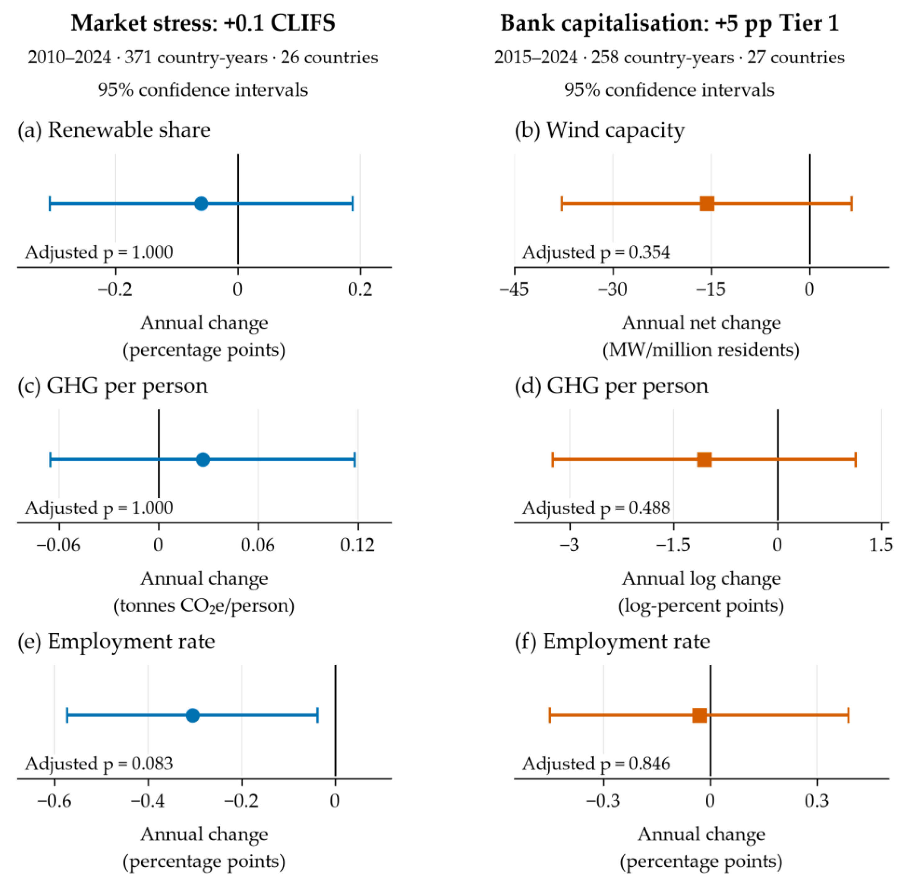
Figure 2.
Associations under outcome-specific controls. Note: Exploratory comparisons use identical country-years within each pair and marginal 95% CR2 intervals. Contrasts are 5 percentage points for Tier 1/NPL and 0.1 CLIFS. Wind/employment use 246 observations; emissions use 238. Tailored stress–employment passes Holm9 (p = 0.015), but not Holm57 (p = 0.093).
Figure 2.
Associations under outcome-specific controls. Note: Exploratory comparisons use identical country-years within each pair and marginal 95% CR2 intervals. Contrasts are 5 percentage points for Tier 1/NPL and 0.1 CLIFS. Wind/employment use 246 observations; emissions use 238. Tailored stress–employment passes Holm9 (p = 0.015), but not Holm57 (p = 0.093).
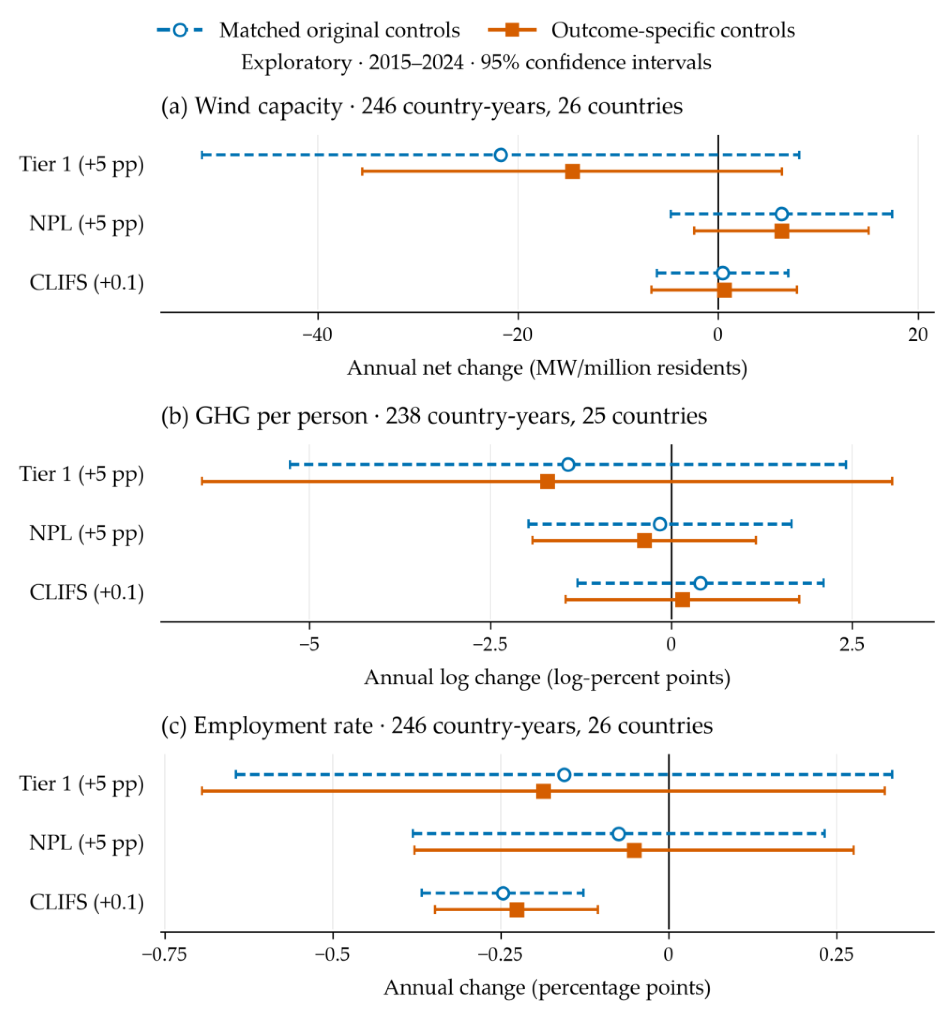
Figure 3.
Aggregate sustainability and its component pattern. Note: Panel (a) gives exploratory annual-index estimates with marginal 95% CR2 intervals; contrasts match Figure 2. Panel (b) shows weighted CLIFS point contributions without intervals; employment supplies 57.3%. Score points are weighted component units. CLIFS passes Holm6 (p = 0.019), but not Holm57 (p = 0.176).
Figure 3.
Aggregate sustainability and its component pattern. Note: Panel (a) gives exploratory annual-index estimates with marginal 95% CR2 intervals; contrasts match Figure 2. Panel (b) shows weighted CLIFS point contributions without intervals; employment supplies 57.3%. Score points are weighted component units. CLIFS passes Holm6 (p = 0.019), but not Holm57 (p = 0.176).
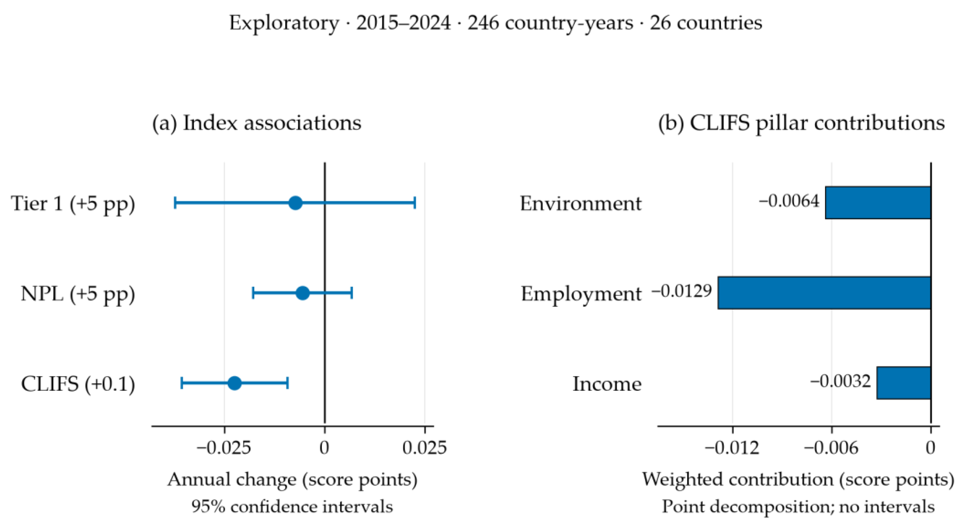
Table 1.
Financial dimensions, outcome definitions and study coverage.
| Measure or outcome | Interpretation | Contrast or change unit | Principal coverage |
|---|---|---|---|
| Tier 1 capital ratio | Bank capitalisation; higher means more Tier 1 capital relative to risk exposure | +5 percentage points | EU27, 258 country-years; 2015–2024 |
| Non-performing loan ratio | Asset quality; higher means a larger gross non-performing loan share | +5 percentage points | Secondary banking and exploratory common panels |
| Country-Level Index of Financial Stress (CLIFS) | Market stress; higher means more stress | +0.1 index units | EU26, 371 country-years; 2010–2024 |
| Renewable-energy expansion | Renewable share in stress models; net wind-capacity change in capital models | Percentage points; MW/million residents | Stress and capital panels, respectively |
| Greenhouse gas emissions per person | Absolute annual change in stress models; annual log change in capital models | Tonnes CO₂e/person; log-percent points | Stress and capital panels, respectively |
| Employment rate, ages 20–64 | Annual employment-rate change | Percentage points | Both principal panels |
Note: All principal models include country and year effects. The exploratory matched panel contains 246 country-years from 26 countries in 2015–2024; tailored emissions models use 238 country-years from 25 countries. Financial measures enter separately and represent distinct constructs. The outcome units and periods differ between the two main outcome groups.
Disclaimer/Publisher’s Note: The statements, opinions and data contained in all publications are solely those of the individual author(s) and contributor(s) and not of MDPI and/or the editor(s). MDPI and/or the editor(s) disclaim responsibility for any injury to people or property resulting from any ideas, methods, instructions or products referred to in the content. |
© 2026 by the authors. Licensee MDPI, Basel, Switzerland. This article is an open access article distributed under the terms and conditions of the Creative Commons Attribution (CC BY) license.
Copyright: This open access article is published under a Creative Commons CC BY 4.0 license, which permit the free download, distribution, and reuse, provided that the author and preprint are cited in any reuse.