
Submitted:
09 November 2026
Posted:
10 November 2026
You are already at the latest version
Abstract
This study investigates Graph Neural Networks (GNNs) for predicting the solvability of finite groups represented by Cayley graphs. A two-layer Graph Convolutional Network (GCN) is employed to learn structural information from these graphs and classify groups as solvable or non-solvable. Experiments on 300 groups consider two settings: S-reserved and A-reserved, in which symmetric and alternating group families, respectively, are excluded from both training and validation. Both settings also include groups from non-reserved families in their test sets. Across 40 random seeds, the GNN achieved mean balanced accuracies of 0.9423 and 0.9014, respectively, outperforming Logistic Regression, Decision Tree, and Random Forest classifiers. Paired one-sided t-tests indicated statistically significant differences in performance relative to all three baselines. Five-fold cross-validation was also conducted to evaluate model stability. These findings suggest that GNNs can capture graph-based structural information relevant to finite-group solvability, with promising results on test sets containing previously unseen group families.
Keywords:
graph neural networks
; finite groups
; solvability
; Cayley graphs
; group classification
; generalization
1. Introduction
Finite groups are traditionally studied through their algebraic operations [1]. Cayley’s theorem [1, Section 4.2] states that every finite group is isomorphic to a subgroup of a symmetric group. Consequently, finite groups can be represented concretely as permutation groups. Among the structural properties of finite groups, solvability [1] occupies a central role in algebra. A group is solvable if it admits a subnormal series with abelian quotients. Examples include cyclic, dihedral, and quaternion groups, whereas symmetric and alternating groups are non-solvable for n ≥ 5.
Let G be a finite group and let S ⊆ G∖{e} be a generating set. The undirected Cayley graph associated with G and S, denoted , is the graph whose vertices correspond to the elements of G, where two vertices are adjacent whenever one is obtained from the other by multiplication by a generator in S [2,3]. Cayley graphs provide a geometric and combinatorial representation of finite groups, encoding algebraic information in a graph structure. This naturally raises the question of whether algebraic properties such as solvability can be inferred directly from these graph representations.
Cayley graphs have been extensively studied for their structural and geometric properties [2,3]. Meanwhile, Graph Neural Networks (GNNs) have demonstrated strong performance on graph-structured data [4,5,6,7,8,9,10]. Despite these advances, the application of GNNs to abstract algebra remains relatively unexplored. In particular, predicting the solvability of finite groups directly from Cayley graphs warrants further investigation.
Motivated by these advances, this study investigates whether a GNN can predict the solvability of finite groups directly from their Cayley graphs, without explicitly using algebraic information such as subgroup structure or the derived series. Experiments are conducted on 300 finite groups using a graph convolutional network (GCN) [7]. Two experimental settings, S-reserved (symmetric-reserved) and A-reserved (alternating-reserved), evaluate generalization by excluding symmetric and alternating group families, respectively, including direct products containing these factors, from both training and validation. In both settings, the test set includes the reserved groups alongside groups from other families. Unlike conventional random splits, these settings assess whether the GNN can generalize to group families not encountered during training or validation.
2. Methodology
This section presents the methodology used to investigate whether GNNs can predict the solvability of finite groups from their associated Cayley graphs. The proposed framework is evaluated under two experimental settings, in which either the alternating or symmetric group family is reserved for testing. Each experiment is repeated across 40 random seeds to assess the robustness of the results. Figure 1 provides an overview of the framework, and the following subsections describe its components and experimental procedures in detail.
1.1. Dataset
The dataset consists of 300 finite groups drawn from seven group families: cyclic, dihedral, quaternion, symmetric, alternating, special linear, and projective special linear groups, together with direct products of groups from these families. Each group is assigned a binary label indicating whether it is solvable. Table 1 summarizes the composition of the dataset.
To evaluate generalization to unseen group families, two experimental settings were considered: S-reserved and A-reserved. In the S-reserved setting, symmetric groups and direct products containing symmetric-group factors were excluded from training and validation and assigned to the test set. Similarly, in the A-reserved setting, alternating groups and direct products containing alternating-group factors were reserved for testing. In both settings, the test set also includes groups from non-reserved families.
In both settings, the dataset was partitioned into training, validation, and test sets using approximately 50%, 20%, and 30% of the groups, respectively. The resulting distributions are summarized in Table 2.
1.2. Generating Sets
For each group family, a generating set was selected to construct the corresponding Cayley graphs. The generating sets used in this study are summarized in Table 3.
1.3. Cayley Graph
For each finite group G, a Cayley graph Γ(G, S) is constructed using a generating set S selected according to the group family. The construction employs breadth-first search (BFS), starting from the identity element e and applying the selected generators.
The Cayley graph Γ(G, S) = (V, E) is undirected and defined by
1.4. GNN Architecture
Overview
The proposed GNN architecture consists of two graph convolutional layers, followed by global mean pooling and two fully connected layers for graph-level classification. The architecture is summarized schematically below, followed by a description of its three main components.
Message Passing → Mean Pooling → Classification
Message Passing. The model employs two graph convolutional layers (GCNConv), based on the Graph Convolutional Network (GCN) propagation mechanism, to learn node representations by aggregating information from neighboring vertices. The first layer transforms the two-dimensional input features into 32-dimensional embeddings, while the second layer produces refined 32-dimensional embeddings. Each convolutional layer is followed by a Gaussian Error Linear Unit (GELU) activation function.
Mean Pooling. Following the graph convolutional layers, global mean pooling aggregates the learned node embeddings into a single graph-level representation by averaging the embeddings of all vertices. The resulting 32-dimensional vector represents the entire graph and serves as input to the classification layers.
Classification. The graph-level embedding is passed through two fully connected linear layers. The first layer maps the 32-dimensional embedding to a 32-dimensional representation, followed by a GELU activation function. The second layer produces two output logits corresponding to the solvable and non-solvable classes.
Message passing
Message passing is the process by which each node aggregates information from its neighboring nodes and updates its feature representation. In the proposed GCN architecture, this process is performed using a degree-normalized weighted sum of neighboring node representations, including the node itself. Specifically, the update rule at layer k is given by:
Mean Pooling
Following the two message-passing layers, each node v has a final feature vector . Let V(G) denote the set of nodes in the Cayley graph G. Mean pooling computes the average of these vectors over all nodes in V(G), producing a single graph embedding
Following mean pooling, the resulting graph embedding zG is passed through two fully connected layers. The first layer applies a linear transformation followed by the GELU activation function, while the second produces two logits corresponding to solvable and non-solvable groups. Specifically,
sG = W2 ⋅ GELU(W1 ⋅ zG + b1) + b2
Here, W1 and W2 are learnable weight matrices, b1 and b2 are bias vectors, and sG contains the two output logits. The predicted class is determined by the larger logit.
1.5. Model Training
The model training procedure consists of three main components: Loss-Function, Backpropagation, and Optimization. The loss function measures the discrepancy between the predicted and true solvability labels. Backpropagation computes the gradients of the loss with respect to the model parameters, while optimization uses these gradients to update the parameters and minimize the loss. The following paragraphs describe each component in detail.
Loss Function. The model uses a class-weighted cross-entropy loss function to measure the difference between predicted and true solvability labels. The weights are calculated as wₛ = N/(2Nₛ) and wₙ = N/(2Nₙ), where Nₛ and Nₙ are the numbers of solvable and non-solvable groups in the training set, respectively, and N = Nₛ + Nₙ. Thus, the class with fewer groups receives a larger weight, reducing the effect of class imbalance during training.
Backpropagation. For each training graph, backpropagation computes the gradients of the loss function with respect to the model’s trainable parameters. These gradients indicate how changes in the parameters affect the loss and are subsequently used by the optimizer to update the model.
Optimization. The model parameters are updated using the Adam optimizer, which uses the gradients computed during backpropagation to minimize the loss function. Parameter updates are performed after processing each training graph. Two training configurations were considered, using 5 and 10 epochs, both with a learning rate of 0.005.
1.6. Evaluation Metrics
The performance of the GCN model was evaluated using two metrics: Balanced Accuracy (BA) [11,13] and Area Under the Receiver Operating Characteristic Curve (AUC). BA was used as the primary metric for selecting the best model, while AUC [14] provided an additional assessment of classification performance. BA is defined as the average recall of the solvable and non-solvable classes:
AUC measures the model’s ability to distinguish between solvable and non-solvable groups across different classification thresholds. An AUC of 1 indicates perfect discrimination, while an AUC of 0.5 corresponds to random discrimination.
3. Results
This section presents the experimental results for two settings: S-reserved, in which symmetric groups are reserved for testing, and A-reserved, in which alternating groups are reserved for testing. In both experiments, the proposed GNN model is compared with Logistic Regression (LR), Decision Tree (DT), and Random Forest (RF) classifiers. Performance is evaluated using BA and ROC-AUC. The baseline classifiers use two graph-level features: the number of vertices and the average vertex degree of each Cayley graph. The baseline classifiers were implemented using scikit-learn. LR was configured with a maximum of 1000 iterations, DT with a maximum depth of 3, and RF with 100 trees. The random state was fixed at 0 for DT and RF. All other hyperparameters retained their default values.
S-reserved Experiment
Test performance and error analysis. Model selection was performed using the validation set described in Table 2, using BA as the selection criterion. The GNN model trained for 5 epochs achieved the highest validation BA (0.9271) and was therefore selected for testing. Table 4 presents its test performance compared with the baseline classifiers.
As shown in Table 4, the GNN achieved the highest BA (BA = 0.9459) and ROC-AUC (1.0000), outperforming all three baseline classifiers. The GNN correctly classified all 53 non-solvable groups and 33 of the 37 solvable groups. The four misclassified groups, all of which are solvable, are presented in Table 5.
Multi seed evaluation. To assess the stability of the results, the experiment was repeated across 40 random seeds. Each seed determined the training, validation, and test split, subject to the reserved-family constraints and fixed proportions of approximately 50%, 20%, and 30%, respectively. For each seed, the GNN model was selected from models trained for 5 and 10 epochs, based on validation BA. Table 6 presents the mean and std of BA and ROC-AUC for the GNN and baseline classifiers.
As shown in Table 6, the GNN achieved the highest mean BA (0.9423) and ROC-AUC (0.9873), outperforming all three baseline classifiers. The relatively low standard deviations indicate consistent performance across the 40 seeds.
Statistical significance. To assess the statistical significance of the GNN’s performance advantage, one-sided paired t-tests were performed against LR, DT, and RF using the BA scores across 40 different random seeds. For each baseline model, the paired differences were defined as
Dᵢ = BA(GNN, i) − BA(baseline, i), i = 1, …, 40,
where baseline denotes LR, DT, or RF, considered separately. The hypotheses were
H₀: μD = 0
H₁: μD > 0
where μD denotes the expected difference in BA. The test statistic was calculated as
All three comparisons rejected H0 (p < 0.001), providing statistically significant evidence that the GNN outperforms LR, DT, and RF in mean balanced accuracy across the 40 random seeds.
Cross validation. To further evaluate the robustness of the GNN model, five-fold stratified cross-validation was performed using the combined training and validation sets, excluding the reserved test set. Table 8 presents the BA and ROC-AUC obtained for each fold, together with their mean values.
A-reserved Experiment
The A-reserved experiment follows the same evaluation procedure as the S-reserved experiment, with alternating groups reserved for testing. The results are presented in Table 9, Table 10, Table 11, Table 12 and Table 13.
Test performance and error analysis. The GNN model was selected based on validation BA. Table 9 compares its test performance with the baseline classifiers.
The GNN achieved the highest BA (0.9357) and AUC (0.9829), outperforming all baseline classifiers. The four misclassified groups are presented in Table 10.
Multi-seed evaluation. The experiment was repeated across 40 random seeds using the same procedure as S-reserved. Table 11 presents the multi-seed performance results.
The GNN achieved the highest mean BA (0.9014) and AUC (0.9781), outperforming all baselines.
Statistical significance. Paired t-tests were performed using BA scores across 40 seeds. Table 12 presents the statistical significance results.
Cross-validation. Five-fold stratified cross-validation was performed using the combined training and validation sets. Table 13 presents the five-fold cross-validation results.
The A-reserved results demonstrate that the GNN outperforms LR, DT, and RF in test performance, with only four misclassified groups. The multi-seed evaluation and statistical significance tests confirm its superior mean performance across random seeds, while the cross-validation results indicate consistently high performance across different data splits.
4. Discussion
Main Findings. In the S-reserved experiment, the GNN achieved a mean BA of 0.9423 and a mean ROC-AUC of 0.9873 across 40 random seeds, outperforming LR, DT, and RF. Statistical tests confirmed that these improvements were significant.
In the A-reserved experiment, the GNN achieved a mean BA of 0.9014 and a mean ROC-AUC of 0.9781 across 40 random seeds, again outperforming all baseline classifiers. Statistical tests confirmed significant improvements over LR, DT, and RF.
Generalization. The S-reserved and A-reserved experiments evaluate the GNN’s ability to generalize to group families excluded from both training and validation. Since the test sets also contain non-reserved groups, the reported performance reflects both types of groups.
Robustness. The multi-seed experiments demonstrate consistent GNN performance across different random seeds, while five-fold cross-validation supports its consistency across different training and validation splits. Together, these results suggest that the model’s performance is stable across random seeds and data splits.
Limitations. The experiments were conducted on 300 finite groups from selected families, limiting the scope of the conclusions. Although the experiments included previously unseen group families, performance on other group families remains untested. Furthermore, the study examined a single GNN architecture and graph representation.
5. Conclusions
This study investigated the use of Graph Neural Networks to predict the solvability of finite groups from their Cayley graphs. Across 40 random seeds, the proposed GCN achieved mean balanced accuracies of 0.9423 and 0.9014 in the S-reserved and A-reserved experiments, respectively, outperforming Logistic Regression, Decision Tree, and Random Forest classifiers. These findings suggest that GNNs can learn structural information relevant to group solvability. The reserved-family experiments provide evidence of generalization, although the test sets contain both reserved and non-reserved groups. Future work will consider additional group families and GNN architectures.
Author Contributions
Tal Weissblat conceived the study, designed the methodology, implemented the graph neural network models, performed the experiments, analyzed the results, and wrote the manuscript.
Funding
No funding was received for this work.
Data Availability Statement
The data and source code supporting the findings of this study are available from the corresponding author upon reasonable request.
Conflicts of Interest
The author declares no conflict of interest.
Declaration of Generative AI Use
Generative AI tools were used solely for language editing. They were not used to generate scientific content, conduct experiments, or analyze results.
References
- Dummit, D. S.; Foote, R. M. Abstract Algebra, 3rd ed.; John Wiley & Sons, 2004. [Google Scholar]
- de la Harpe, P. Topics in Geometric Group Theory. In Chicago Lectures in Mathematics; University of Chicago Press: Chicago, 2000. [Google Scholar]
- Konstantinova, E. Some Problems on Cayley Graphs. In Linear Algebra and its Applications; 2008; vol. 429, pp. 2754–2769. [Google Scholar]
- Bronstein, M. M.; Bruna, J.; Cohen, T.; Veličković, P. Geometric Deep Learning: Grids, Groups, Graphs, Geodesics, and Gauges. arXiv 2021, arXiv:2104.13478. [Google Scholar]
- Wu, Z.; Pan, S.; Chen, F.; Long, G.; Zhang, C.; Yu, P. S. A Comprehensive Survey on Graph Neural Networks. IEEE Trans. Neural Netw. Learn. Syst. 2021, vol. 32(no. 1), 4–24. [Google Scholar] [CrossRef] [PubMed]
- Scarselli, F.; Gori, M.; Tsoi, A. C.; Hagenbuchner, M.; Monfardini, G. The Graph Neural Network Model. IEEE Trans. Neural Netw. 2009, vol. 20(no. 1), 61–80. [Google Scholar] [CrossRef] [PubMed]
- Kipf, T. N.; Welling, M. Semi-Supervised Classification with Graph Convolutional Networks. In Proceedings of the International Conference on Learning Representations (ICLR), 2017. [Google Scholar]
- Xu, K.; Hu, W.; Leskovec, J.; Jegelka, S. How Powerful are Graph Neural Networks? In Proceedings of the International Conference on Learning Representations (ICLR), 2019. [Google Scholar]
- Gilmer, J.; Schoenholz, S. S.; Riley, P. F.; Vinyals, O.; Dahl, G. E. Neural Message Passing for Quantum Chemistry. In Proceedings of the 34th International Conference on Machine Learning (ICML), PMLR, 2017; vol. 70, pp. 1263–1272. [Google Scholar]
- Ying, R.; You, J.; Morris, C.; Ren, X.; Hamilton, W. L.; Leskovec, J. Hierarchical Graph Representation Learning with Differentiable Pooling. Adv. Neural Inf. Process. Syst. (NeurIPS) 2018, vol. 31, 4894–4904. [Google Scholar]
- García, V.; Mollineda, R. A.; Sánchez, J. S. “Index of Balanced Accuracy: A Performance Measure for Skewed Class Distributions,” in Pattern Recognition and Image Analysis. In Lecture Notes in Computer Science; Springer: Berlin, Heidelberg, 2009; vol. 5524, pp. 441–448. [Google Scholar] [CrossRef]
- Fey, M.; Lenssen, J. E. Fast Graph Representation Learning with PyTorch Geometric. ICLR Workshop on Representation Learning on Graphs and Manifolds, 2019. [Google Scholar]
- Brodersen, K. H.; Ong, C. S.; Stephan, K. E.; Buhmann, J. M. The Balanced Accuracy and Its Posterior Distribution. In Proceedings of the 20th International Conference on Pattern Recognition (ICPR), 2010; pp. 3121–3124. [Google Scholar]
- Fawcett, T. An Introduction to ROC Analysis. Pattern Recognit. Lett. 2006, vol. 27(no. 8), 861–874. [Google Scholar] [CrossRef]
Figure 1.
Overview of the proposed framework for predicting the solvability of finite groups from their associated Cayley graphs using GNN.
Figure 1.
Overview of the proposed framework for predicting the solvability of finite groups from their associated Cayley graphs using GNN.
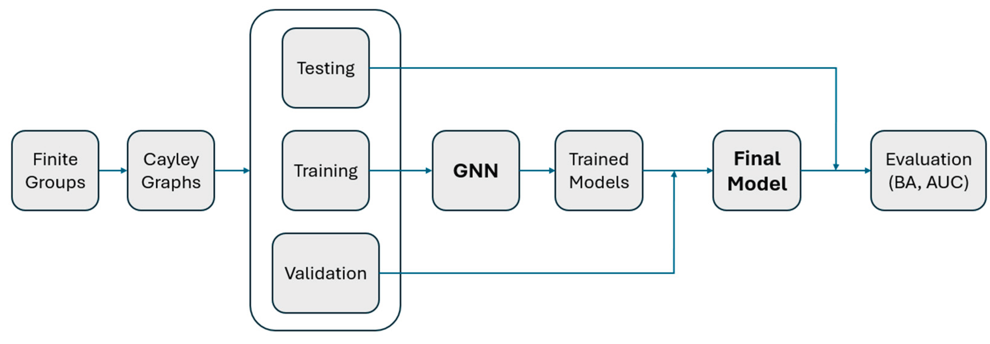

Table 1.
Benchmark dataset composition by group family.
| Family | Notation | Number of groups |
| Cyclic | Cn | 23 |
| Dihedral | Dn | 41 |
| Quaternion | 5 | |
| Symmetric | Sn | 3 |
| Alternating | An | 4 |
| Special Linear | SL(2,q) | 5 |
| Projective Special Linear | PSL(2,q) | 6 |
| Direct Products | G × H | 213 |
| Total | 300 |
Table 2.
Dataset distributions for the S-reserved and A-reserved experiments.
| Experiment | Split | Pos. | Neg. | Total | % Pos | % Neg | % Total |
| S-reserved | Train | 104 | 45 | 149 | 69.8% | 30.2% | 49.7% |
| Valid | 43 | 18 | 61 | 70.5% | 29.5% | 20.3% | |
| Test | 37 | 53 | 90 | 41.1% | 58.9% | 30.0% | |
| Total | 184 | 116 | 300 | 61.3% | 38.7% | 100.0% | |
| A-reserved | Train | 116 | 33 | 149 | 77.9% | 22.1% | 49.7% |
| Valid | 48 | 13 | 61 | 78.7% | 21.3% | 20.3% | |
| Test | 20 | 70 | 90 | 22.2% | 77.8% | 30.0% | |
| Total | 184 | 116 | 300 | 61.3% | 38.7% | 100.0% |
Table 3.
Generating sets and generator properties for the group families.
| Group | Generating set | Generator properties |
| Cn | {r, r−1} | rn = e |
| Dn | {r, r−1, s} | rn = s2 = e, srs = r−1 |
| {a, a−1, b, b−1} | ||
| Sn | {a, a−1, b, b−1} | a = (1 2), b = (1 2 ... n), a2 = bn = e |
| An | {a, a−1, b, b−1} |
n odd: a = (1 2 3),b = (1 2...n), a3 = bn = e n even: a = (1 2 3),b = (2 3 ... n),a3 = bn−1 = e |
| SL(2,q) | {A, A−1, B, B−1} | {A = [[1,1],[0,1]],B = [[0,−1],[1,0]]} det(A) = det(B) = 1 q is prime; matrix operations are modulo q |
| PSL(2,q) | {A, A−1, B, B−1} | {A = [[1,1],[0,1]], B = [[1,0],[1,1]]} det(A) = det(B) = 1, M∼−M(mod q) q is prime; matrix operations are modulo q |
| G × H | SG×H = (SG × {eH}) ∪ ({eG} × SH) | (g,h)(g',h') = (gg',hh') |
Table 4.
Test performance (S-reserved).
| Model | TP | FN | TN | FP | BA | AUC |
| GNN | 33 | 4 | 53 | 0 | 0.9459 | 1.0000 |
| LR | 36 | 1 | 4 | 49 | 0.5242 | 0.6652 |
| DT | 29 | 8 | 53 | 0 | 0.8919 | 0.9735 |
| RF | 31 | 6 | 43 | 10 | 0.8246 | 0.8774 |
Table 5.
Misclassified groups (S-reserved).
| Group | True | Pred | Prob |
| D2xS4 | 1 | 0 | 0.4210 |
| C3xQ32 | 1 | 0 | 0.3831 |
| D4xQ16 | 1 | 0 | 0.3452 |
| C4xQ32 | 1 | 0 | 0.2737 |
Table 6.
Multi-seed performance (S-reserved).
| Statistic | BA | AUC | ||||||
| GNN | LR | DT | RF | GNN | LR | DT | RF | |
| Mean | 0.9423 | 0.4735 | 0.8460 | 0.8131 | 0.9873 | 0.6584 | 0.9451 | 0.8934 |
| Std | 0.0256 | 0.0270 | 0.0453 | 0.0405 | 0.0147 | 0.0581 | 0.0352 | 0.0399 |
Table 7.
Statistical significance (S-reserved).
| Comparison | Mean Difference | Std | t-statistic | p-value |
| GNN vs LR | 0.4688 | 0.0398 | 74.5563 | 5.54 × 10−44 |
| GNN vs DT | 0.0963 | 0.0519 | 11.7331 | 1.15 × 10⁻¹⁴ |
| GNN vs RF | 0.1292 | 0.0510 | 16.0157 | 4.80 × 10⁻¹⁹ |
Table 8.
Five-fold cross-validation (S-reserved).
| Fold | BA | AUC |
| 1 | 0.9333 | 0.9639 |
| 2 | 0.9333 | 0.9806 |
| 3 | 0.9098 | 0.9337 |
| 4 | 0.8117 | 0.9284 |
| 5 | 0.9828 | 1.0000 |
| Mean | 0.9142 | 0.9613 |
Table 9.
Test performance (A-reserved).
| Model | TP | FN | TN | FP | BA | AUC |
| GNN | 18 | 2 | 68 | 2 | 0.9357 | 0.9829 |
| LR | 20 | 0 | 6 | 64 | 0.5429 | 0.7789 |
| DT | 20 | 0 | 6 | 64 | 0.5429 | 0.5643 |
| RF | 20 | 0 | 7 | 63 | 0.5500 | 0.7007 |
Table 10.
Misclassified groups (A-reserved).
| Group | True | Pred | Prob |
| A5 | 0 | 1 | 0.5718 |
| C3xA5 | 0 | 1 | 0.5132 |
| C60xQ8 | 1 | 0 | 0.1948 |
| D27 | 1 | 0 | 0.2882 |
Table 11.
Multi-seed performance (A-reserved).
| Statistic | BA | AUC | ||||||
| GNN | LR | DT | RF | GNN | LR | DT | RF | |
| Mean | 0.9014 | 0.5058 | 0.5538 | 0.5567 | 0.9781 | 0.8216 | 0.5500 | 0.6709 |
| Std | 0.0413 | 0.0134 | 0.0105 | 0.0068 | 0.0188 | 0.0548 | 0.0209 | 0.0598 |
Table 12.
Statistical significance (A-reserved).
| Comparison | Mean difference | Std | t-statistic | p-value |
| GNN vs LR | 0.3956 | 0.0448 | 55.8050 | 4.03 × 10−39 |
| GNN vs DT | 0.3477 | 0.0422 | 52.1261 | 5.56 × 10−38 |
| GNN vs RF | 0.3447 | 0.0416 | 52.4571 | 4.36 × 10−38 |
Table 13.
Five-fold cross-validation (A-reserved).
| Fold | BA | AUC |
| 1 | 1.0000 | 1.0000 |
| 2 | 0.9697 | 0.9865 |
| 3 | 1.0000 | 1.0000 |
| 4 | 1.0000 | 1.0000 |
| 5 | 0.9187 | 0.9781 |
| Mean | 0.9777 | 0.9929 |
Disclaimer/Publisher’s Note: The statements, opinions and data contained in all publications are solely those of the individual author(s) and contributor(s) and not of MDPI and/or the editor(s). MDPI and/or the editor(s) disclaim responsibility for any injury to people or property resulting from any ideas, methods, instructions or products referred to in the content. |
© 2026 by the authors. Licensee MDPI, Basel, Switzerland. This article is an open access article distributed under the terms and conditions of the Creative Commons Attribution (CC BY) license (http://creativecommons.org/licenses/by/4.0/).
Copyright: This open access article is published under a Creative Commons CC BY 4.0 license, which permit the free download, distribution, and reuse, provided that the author and preprint are cited in any reuse.