
Submitted:
06 November 2026
Posted:
10 November 2026
You are already at the latest version
Abstract
Counting how many vehicles crossed an intersection produces a report; finding which vehicles move together, and through which cameras, reveals the structure of urban traffic. License plate recognition cameras make that structure observable. Sets of cameras frequently shared by the same vehicles expose the corridors that traffic actually uses, and groups of vehicles repeatedly seen together at the same cameras support automated convoy detection for traffic enforcement. Both are frequent itemset mining problems, and they are precisely where relational databases lose ground as data grow. We quantify that loss for the corridor formulation, comparing a self join in indexed PostgreSQL with distributed FP-Growth on a four-worker Apache Spark cluster over 100 million simulated detections from 500 cameras on the road network of Pereira, Colombia, at eight nested scales from 50 thousand to 15 million rows. For reports, histograms, lookups and alerts, PostgreSQL wins at every scale by up to five orders of magnitude, and Spark never leaves a fixed overhead of two to four minutes. Structure mining behaves differently: the relational advantage collapses from 328 to 1.6 times, because the self join grows super-linearly while FP-Growth grows almost linearly. Extrapolated growth exponents place the crossover between 30 and 73 million detections, four to nine days of operation, which tells a city when structural analysis must move off the relational engine.
Keywords:
frequent itemset mining
; FP-Growth
; license plate recognition
; big data architectures
; Apache Spark
; PostgreSQL
; intelligent transportation systems
; scalability benchmark
; smart cities
1. Introduction
Smart city programmes increasingly instrument the road network with cameras whose primary purpose is enforcement, but whose by-product is a dense, structured record of vehicle movement [1,2]. Once each frame has been reduced to a tuple containing a timestamp, a camera identifier and a license plate, the camera network stops being a video problem and becomes a data problem, with the volume, velocity and variety that characterise big data workloads [3,4,5]. Automatic number plate recognition (ANPR) data of this kind already support travel-time estimation, queue estimation, origin–destination inference and trajectory reconstruction [6,7,8,9]. In a mid-sized Colombian city such as Pereira, a deployment of a few hundred cameras would produce tens of millions of detections per week, a volume at which the choice of storage and query engine stops being an implementation detail and starts determining which questions can be asked at all.
Among the questions a traffic authority can pose over such a stream, the most valuable are not the ones that count events but the ones that reveal structure. Knowing how many vehicles passed a given intersection last Tuesday is a report. Knowing which groups of cameras are frequently traversed by the same vehicles describes the corridors that traffic actually uses, which supports signal coordination and enforcement planning. The same reasoning applied the other way round, to the groups of vehicles that repeatedly pass the same cameras together, is the basis of automated convoy detection, a direct tool for traffic enforcement [10]. Formally, both questions are instances of frequent itemset mining [11,12]. In the first, each plate is a transaction and each camera an item, and a frequent itemset is a set of cameras that recurs with at least a specified support; in the second, the roles are exchanged, with camera and time windows as transactions and plates as items. This paper measures the first formulation. The second shares its cost structure, and because a busy camera window contains many more plates than a single plate has detections, its relational cost per transaction is expected to be even higher.
The engineering difficulty is that this workload sits exactly at the boundary between the two families of engine that a smart city platform typically has available [13,14]. On one side, a relational database management system materialises the detections in indexed tables, paying once for extraction, loading and index construction, and thereafter touching only the rows relevant to each query. On the other, a distributed processing engine reads columnar files directly and parallelises the computation across workers, investing nothing up front but rescanning the data on every query [15,16,17]. The received wisdom is that the distributed engine wins when data are large, but at what volume, for which query, and under which cluster topology this actually happens is rarely reported with enough detail to support a sizing decision.
This paper answers that question for the frequent itemset workload specifically. The contribution is threefold. First, a reproducible benchmark that measures five decision-making workloads on an indexed PostgreSQL instance and on a four-worker Spark cluster across eight nested data scales spanning almost three orders of magnitude. Second, a characterisation of the fixed coordination overhead that dominates the distributed engine below roughly one million rows, which explains why the naive expectation of distributed superiority fails at moderate volumes. Third, and centrally, a quantitative account of the frequent itemset workload as the only one in the suite whose engine preference is projected to invert with scale, together with an extrapolated crossover volume derived from the fitted growth exponents of the two curves.
One caveat frames every number that follows: the whole benchmark ran on a single machine, where the four Spark workers share the disk and memory bandwidth of one host. Independent I/O paths on real distributed hardware would improve the behaviour of the cluster, so the distributed engine is reported here under a handicap it would not face in a physical deployment. The remainder of the paper is organised as follows. Section 2 reviews related work, Section 3 describes the dataset, the two implementations and the experimental protocol, Section 4 presents the measurements, Section 5 discusses their architectural implications and limitations, and Section 6 concludes.
2. Related Work
2.1. License Plate Recognition Data in Smart Cities
ANPR cameras are deployed mainly for law enforcement and toll collection, but because they are often owned by the authorities that would use their data, they have become an inexpensive source of vehicle-level mobility information [8]. Published uses include travel-time and queue-length estimation [6], origin–destination estimation from reconstructed trajectories [7], trajectory reconstruction from sparse camera networks [9], the regularity of individual vehicle arrivals [18] and the detection of vehicles travelling in convoy [10]. Hadavi et al. analysed two weeks of data from 122 cameras in a Belgian police district and showed that camera-pair frequencies recover the main corridors also seen in GPS data [8]. These studies share a methodological focus: they describe what can be learned from the data, and treat the storage and processing infrastructure as given. Surveys of big data for traffic estimation note that the tooling question remains comparatively under-examined [14], and architectural proposals for smart city transport combine stream and batch layers without quantifying where the boundary between them should lie [13]. The present work addresses that gap for one specific and computationally demanding question.
2.2. Frequent Itemset Mining
The problem was formalised by Agrawal and Srikant in the context of association rule discovery over retail baskets. Their Apriori algorithm exploits the downward closure property of support, generating candidate itemsets of increasing cardinality and pruning any candidate with an infrequent subset [11]. The cost of Apriori is dominated by repeated candidate generation and by one database pass per level, which becomes prohibitive when transactions are long or support thresholds low. Han et al. removed candidate generation altogether with FP-Growth, which compresses the transaction database into a prefix tree of frequent items, the FP-tree, and mines it recursively by projecting conditional pattern bases [12]. FP-Growth requires two passes over the data and scales substantially better; its parallel formulation, PFP [19], is the basis of the implementation in the MLlib package of Apache Spark [20]. A broad survey of the itemset mining family is given in [21], and the relation between itemsets and trajectory patterns is discussed in [22].
A third route exists that is rarely discussed in the mining literature because it belongs to the database tradition: expressing co-occurrence directly in relational algebra. A self join of the transaction table with itself, keyed on the transaction identifier and constrained to avoid duplicate pairs, enumerates every co-occurring pair of items and counts them in a single declarative statement. This route requires no specialised library and benefits from decades of query optimiser engineering, but it materialises a quadratic number of intermediate tuples per transaction and does not generalise gracefully beyond pairs. Understanding when this pragmatic option stops being viable is precisely the practical question faced by an engineering team that already operates a relational database.
2.3. Query Engines and Processing Regimes
The distinction between transactional and analytical processing regimes is long established. Online transaction processing is characterised by many short, selective operations over few rows and benefits from indexed access paths; online analytical processing aggregates over large row counts and prioritises efficient scanning over the latency of any individual operation [17]. Column-oriented storage was introduced specifically to serve the second regime [23], and the columnar file formats used by contemporary distributed engines are its direct descendants.
The distributed lineage begins with MapReduce [15] and its distributed file system [24], and continues with in-memory engines that retain fault tolerance while avoiding disk materialisation between stages [16,25], including a relational layer over the same runtime [26]. Whether parallel databases or MapReduce-style systems are the better substrate for analytical work was debated explicitly by Pavlo et al., whose benchmark found well-tuned parallel databases faster on most analytical tasks at the cost of longer loading times [27,28]; the trade-off between paying for loading once and rescanning on every query is the same one examined here. On the streaming side, structured streaming models an unbounded stream as an incrementally executed relational query [29], and the Kappa architecture argues for a single streaming substrate [30] in place of the separate batch and speed layers of the Lambda architecture [31]. Comparative benchmarking of these engines has focused predominantly on streaming latency and throughput [32], leaving the batch analytical regime, and mining workloads in particular, comparatively under-measured against a well-tuned relational baseline.
2.4. From Video to Detections
The event stream analysed here is the output of a computer vision pipeline whose components are mature (Figure 1a). Single-stage detectors process video at real-time rates [33], and the YOLOv8 family is a current practical choice for plate localisation [34]. Tracking-by-detection associates detections across frames to preserve identity, with the SORT family and its appearance-aware and low-confidence extensions being the standard options [35,36]. Optical character recognition then converts the plate crop into a string [37], and multi-camera vehicle datasets such as CityFlow [38] establish benchmark conditions for city-scale deployments. This work takes the existence of such a pipeline as given and concerns itself exclusively with what happens downstream, once detections have been persisted.
3. Materials and Methods
3.1. Synthetic Detection Dataset
Real detections at the volume required are not obtainable, both because no such archive was available and because license plate records carry privacy restrictions. The dataset was therefore produced by a microscopic traffic simulation over the real road network of Pereira, Risaralda, Colombia. The simulation is microscopic in the usual sense of the term [39]: each vehicle is an individual agent with its own origin, destination, route and speed, rather than an aggregate flow density. That granularity is what makes the dataset usable here, since each camera emits its own independent detection stream and the co-visitation structure emerges from individual trajectories rather than being imposed by the generator. The road graph is downloaded from OpenStreetMap through the OSMnx library restricted to drivable ways [40], and only its largest strongly connected component is retained so that every origin can reach every destination; each edge carries its speed limit, length and traversal time.
Five hundred cameras are placed on the nodes of highest betweenness centrality [41], that is, the intersections through which the largest number of shortest paths pass, mirroring the criterion an urban planner would apply when siting enforcement cameras (Figure 2). Each vehicle receives a random origin and destination and follows the time-shortest path; it is assigned a type (car with probability , motorcycle , truck ), a colour, a uniform speed in km/h and a plate in the Colombian format, ABC123 for cars and trucks and ABC12D for motorcycles. A route completion probability distributed as models vehicles that abandon their planned trajectory, reproducing unanticipated turns.
The simulation advances in discrete steps of s with between and concurrent vehicles. When a vehicle crosses a camera-equipped node, a detection event is emitted with ten fields: timestamp, camera identifier, plate, internal vehicle identifier, graph node and edge, speed, vehicle type, colour and heading. Output is persisted as Hive-partitioned Parquet by year/month/day/hour, which enables temporal predicate pushdown, using a fixed seed and checkpointing every events for reproducibility. Table 1 summarises the window actually loaded for the benchmark; every evaluated scale is a nested temporal sub-window of this range, all starting at the same instant.
Three properties of this dataset matter for the mining workload. First, the mean number of detections per plate over the full window is , so transactions are short but not trivially so. Second, because every scale is a window that opens at the same instant, short windows cut trips that are still in progress and therefore contain truncated, shorter transactions; the mean transaction length grows with the window until the window comfortably exceeds the typical trip duration. At the generation rate of Table 1, the smallest scale of 50 thousand rows corresponds to roughly nine minutes of simulated traffic and the 1 million row scale to about three hours. Third, the camera population is fixed at 500 items, so the itemset lattice does not grow with the data volume; only the transaction database does.
The dataset is synthetic, and its mobility is not calibrated against observed counts. Origins and destinations are drawn at random and plates do not recur across trips, so the frequent itemsets it yields reflect the shortest-path structure of the network around high-centrality intersections rather than the habitual behaviour of real drivers. This is adequate for the purpose of the study, which is to measure the computational cost of mining as a function of volume, because that cost depends on the number and length of transactions and not on their semantic content. It does mean that the mined itemsets themselves should not be read as findings about traffic in Pereira.
3.2. Problem Formulation
Let D be the set of detections, each a tuple of plate, camera and timestamp. The transaction database is obtained by grouping detections by plate,
where P is the set of distinct plates. Cameras are the items and each plate contributes one transaction consisting of the set of cameras it was seen at, with multiplicity discarded (Figure 1b). The support of an itemset is its relative frequency among transactions,
and the mining task is to return every X with for a threshold , fixed here at . A frequent itemset of cardinality two or more is, in this domain, a set of cameras traversed together by at least five percent of the observed vehicles.
3.3. The Two Implementations
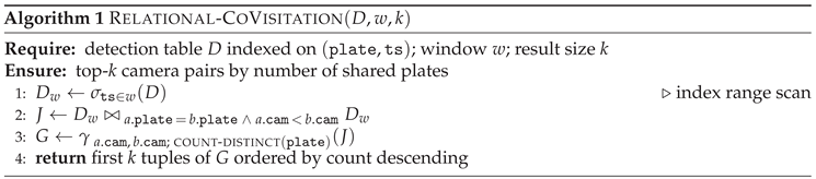
The relational implementation expresses pairwise co-visitation directly, joining the detection table with itself on the plate and breaking the symmetry with a strict inequality on the camera identifier, as sketched in Algorithm 1. It is declarative, requires no library beyond the database, and exploits the index on to restrict the scan to the temporal window. Its cost, however, is governed by the number of intermediate tuples it materialises. For a plate observed times the join emits pairs, so the total intermediate volume is
with and the first and second moments of the per-plate detection count. This is the precise sense in which the self join is quadratic: it is quadratic in the detections per transaction, not in the global row count. Equation (3) therefore predicts a measured growth exponent above one only while is still growing with the window, which in this dataset happens while windows are short enough to truncate trips. Once the transaction length distribution stabilises, Equation (3) predicts linear growth, and any additional steepening must come from the physical cost of materialising and aggregating the intermediate tuples rather than from their number.
 |
The distributed implementation, sketched in Algorithm 2, builds the transaction database of Equation (1) explicitly with a shuffle-based grouping and hands it to the FP-Growth implementation of MLlib [12,19,20]. It reads the Parquet files directly, with no prior loading or indexing of any kind, and relies on partition pruning for the temporal filter.
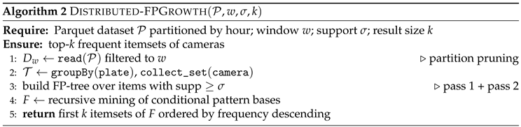 |
The two implementations are deliberately not equivalent in output, and the asymmetry favours the relational side. The self join solves only the pairwise case, enumerating co-visited camera pairs, whereas FP-Growth mines itemsets of arbitrary cardinality and additionally returns the frequent singletons. The relational engine is therefore given the strictly easier problem, and any erosion of its advantage with scale is a conservative estimate of the advantage of the distributed formulation. Where the outputs do overlap, on the support of pairs, their agreement is checked at every scale as described in Section 4.4.
3.4. Workload Suite
Frequent itemset mining is measured alongside four other workloads, listed in Table 2, chosen so that the suite covers the decision-making primitives an operational camera platform must serve: reports, distribution histograms, individual lookups and alerts. Their role in this study is diagnostic. Because they exercise the same two engines over the same data at the same scales but with radically different computational profiles, they separate the fixed cost of each engine from the data-dependent cost, which is what makes the behaviour of the mining workload interpretable. Each workload was implemented twice, in SQL and in PySpark, and the two implementations were verified to produce identical results at every scale.
3.5. Storage Configurations
The comparison contrasts two radically different storage philosophies, shown end to end in Figure 3. In PostgreSQL 16 the data are materialised in a relational table range-partitioned by month on the timestamp, over which three indexes are built, , and , tailored to the evaluated queries. Loading is performed by an ETL process that copies the Parquet into the table with COPY, dropping the indexes before the bulk load and recreating them at the end. In Apache Spark 3.5.8 there is no prior loading of any kind: the engine reads the hour-partitioned Parquet files directly and has no indexes.
This asymmetry is the interpretive key to the whole experiment. PostgreSQL pays once for the ETL and the indexing and thereafter answers each query touching only the pertinent rows; Spark invests nothing up front but rescans the relevant Parquet on every query. The reported times exclude the one-off ETL and index construction cost entirely, which is again a choice that favours the relational engine.
3.6. Execution Environment
The Spark cluster is brought up with Docker Compose on a single host of 24 threads and 80 GB of memory, on an internal network shared with PostgreSQL. It comprises one master and four workers of four cores and 12 GB each, totalling 16 cores and 48 GB of execution capacity, plus a client node acting as driver; each executor operates with a 10 GB heap and four cores, with spark.cores.max and 400 shuffle partitions. No dataset was cached between queries. PostgreSQL 16 ran with shared_buffers4 GB, work_mem256 MB, effective_cache_size12 GB and max_parallel_workers_per_gather4. As an infrastructure constraint worth recording, the default WSL2 configuration caps memory at fifty percent of the host, which is insufficient to sustain the cluster; it had to be raised to 64 GB through the .wslconfig file to avoid termination by memory exhaustion.
Two consequences of this topology must be stated before the results are read. First, as anticipated in the introduction, the four workers share CPU, memory and disk bandwidth, so the measurements are a lower bound on the benefit of the distributed solution relative to a multi-machine cluster. Second, PostgreSQL runs on the same host and thus competes for the same resources, which is symmetric in principle but favours the engine with the smaller working set.
3.7. Measurement Protocol
The protocol is a systematic sweep over a scalability ladder. Each scale is defined as a temporal window which, at the rate of M rows per day, yields the target volume; the evaluated scales are s50K, s100K, s150K, s200K, s500K, s1M, s10M and s15M, all beginning at the same instant so that each is nested in the next. For PostgreSQL each cell is executed three times and the median reported, preceded by a warm-up run; for Spark a single repetition is executed, a decision justified by the low variance of its overhead floor, below two percent between repetitions in prior tests, and which allows the sweep to complete in about three hours instead of twelve.
Only the execution of the workload is timed, that is, the filter, the computation and the collection of the result, using time.perf_counter; the start-up of the Spark session and the opening of the PostgreSQL connection are left outside the clock. The complete design spans eight scales, five workloads and two engines, producing eighty measurement cells from 160 timed runs. Raw results are persisted as CSV, from which a single script regenerates every figure and table without Spark or Docker. Growth exponents are obtained by ordinary least squares on against ; over a segment with only two scales the fit reduces to the slope between the two points.
4. Results
Table 3 consolidates the eighty measurement cells and Figure 4 presents the corresponding curves. The first observation is blunt: over the entire evaluated range and in all five workloads, indexed PostgreSQL responds faster than Spark. No crossover is observed below 15 M rows in any workload.
4.1. The Fixed Overhead Floor of the Distributed Engine
Spark exhibits a fixed overhead floor. In W1, W2 and W4 its response time is essentially constant between 50 K and 1 M rows, with medians of 124, 126 and 125 s respectively and spreads of at most 27 s across a twentyfold change in data volume. In W3 and W5, which require an additional shuffle pass, the floor sits higher, at medians of 243 and 248 s. Within this regime the size of the data is irrelevant against the fixed cost of planning the job, launching tasks on the four workers and rescanning the Parquet. The data only begin to matter from the s10M scale onwards. PostgreSQL, by contrast, starts from sub-millisecond times and grows smoothly. Figure 5 contrasts the two behaviours on the lightest and the heaviest workload.
The extreme case is W3, the trajectory of a single plate. PostgreSQL resolves an index seek on in a median of ms at any scale, while Spark requires a full scan taking a median of 242 s, a difference of roughly that remains constant across the ladder. Reading up to 10.8 GB to return a handful of rows is pure waste, and this is a consequence of the distributed execution model rather than a configuration defect.
4.2. Frequent Itemset Mining
W5 is the only workload whose engine preference is in motion. Table 4 and Figure 6 give its detail. The relational self join goes from s at s50K to s at s15M, growing by a factor of 821 while the data grow by a factor of 300. Distributed FP-Growth, in contrast, stays pinned to its floor between 231 and 261 s over the first six scales and only then begins to climb, reaching s at s15M.
The consequence is a monotone erosion of the relational advantage, quantified in Figure 7 as the ratio of Spark time to PostgreSQL time. That ratio falls from at s50K to , , , and , and then to at s10M and at s15M. Over a 300-fold increase in volume the relative advantage of the relational engine contracts by a factor of two hundred.
The ratio erodes in the other workloads too, from to in W1, from to in W2 and from to in W4, while staying flat near in W3. Those erosions, however, are artifacts of the flat overhead floor rather than evidence about marginal cost: at s15M the distributed engine is still on its floor in W1, W2 and W4, at 121, 108 and 112 s, so its curve has not yet begun to respond to the data at all. W5 is the only workload in the suite where the distributed engine has demonstrably left its floor within the measured range, rising to 684 s and s at the last two scales, and where the ratio nevertheless keeps falling. It is therefore the only workload for which both engines’ marginal costs are simultaneously observable and the comparison of growth rates is meaningful.
4.3. Growth Exponents and Extrapolated Crossover
Fitting a power law on the log–log curves quantifies the two growth regimes (Table 5). For the relational self join the exponent is over the full ladder, over and between the last two scales. This is the highest relational exponent in the suite: the same fit over the full ladder gives for W4, for W1, for W2 and for the indexed lookup of W3. For distributed FP-Growth the exponent over is only , but this figure is contaminated by the overhead floor at s1M and understates the marginal cost; between the last two scales, where the floor no longer dominates, the exponent is , that is, close to linear.
The super-linear and increasing relational exponent has two plausible sources, and the present data do not fully separate them. At the bottom of the ladder, where windows last minutes and truncate most trips, the mean transaction length grows with the window and Equation (3) accounts for super-linear growth directly. At the top of the ladder, windows of 30 to 45 hours are much longer than any trip, the transaction length distribution should be close to stationary, and Equation (3) by itself predicts linear growth. The steepening to between s10M and s15M is therefore more plausibly a physical effect of the join than a combinatorial one: on the order of intermediate pairs must be hashed and aggregated, which can exceed the 256 MB of work_mem available to each hash operation and force spilling to disk, on a host whose memory is shared with the Spark workers. Either way the effect is real for the hardware measured, but its origin matters for extrapolation, and Section 5 returns to it.
Extrapolating the two fits from the last measured point, where the ratio is , gives the crossover volume at which the curves meet:
Using the exponents, and rows; using the wider window, where the difference is , . The crossover therefore lies between roughly thirty and seventy-three million detections, that is, between four and nine days of operation for this five-hundred-camera deployment. The spread between the two estimates reflects genuine sensitivity to the fitting window, and the narrower window rests on two points per engine, so the bracket should be read as an order-of-magnitude estimate rather than a precise threshold.
4.4. Cross-Validation of the Mined Patterns
Because the two implementations mine the same patterns by entirely different means, their agreement is a useful correctness check on the two code paths. The check is deliberately narrow in scope: at each of the eight scales, the support of the top-ranked pair returned by the relational self join was compared against the frequency of the top-ranked two-item itemset returned by FP-Growth. The two agree exactly at all eight scales, with counts of 404, 704, , , , , and shared plates respectively. This establishes that the SQL and the PySpark code paths compute the same quantity, so the timing comparison is one of cost rather than of semantics. It does not verify the complete result set: only the leading itemset of each run was retained, and extending the check to the full top-k lists is left for a future sweep.
5. Discussion
Three findings follow from these measurements, and their joint reading is an architectural recommendation rather than an engine preference.
The first is that a distributed engine is structurally unsuited to small and medium query volumes, and this has little to do with tuning. Below roughly one million rows the response time is independent of data size and dominated by job planning, task distribution and Parquet rescanning. In this regime the relational engine wins by factors ranging from tens to hundreds of thousands. Any architecture that routes interactive or operational queries through a distributed batch engine pays a two-minute floor for answers a relational index would return in milliseconds. This is consistent with the earlier finding that well-tuned parallel databases outperform MapReduce-style systems on most analytical tasks once their loading cost has been paid [27].
The second is that the dominance of the relational engine over the rest of the suite stems from its storage model. It invests once in ETL and index construction, and thereafter every query touches only the pertinent rows; the distributed engine rescans on every query. For the operational queries typical of a city the size of Pereira, such as reports by camera, re-identification alerts and plate lookups over windows of hours or a few days, a partitioned and indexed relational schema answers in milliseconds to tens of seconds, orders of magnitude below the distributed alternative.
The third finding is the substantive one. Frequent itemset mining reveals the regime where the balance begins to tip. Its relational cost is governed by the volume of intermediate pairs and by the cost of aggregating them, which is why its exponent is the highest in the suite and keeps rising across the measured range. Distributed FP-Growth, by contrast, grows close to linearly once its floor is paid, and two curves with different exponents must eventually cross. The relational engine reached this point while solving only the pairwise case and without being charged for its ETL and indexing; a fair accounting on either axis would move the crossover earlier.
The practical reading is therefore a hybrid architecture consistent with the Lambda and Kappa patterns [13,29,30,31]. An indexed relational engine should serve as the serving layer for interactive queries, near-real-time alerts and point lookups, where its indexed access is unbeatable. A distributed engine should be reserved for massive batch analytics, co-visitation mining over months of data and model retraining, where its parallelism and direct columnar reads repay the fixed coordination cost. The exponents reported here turn that qualitative recommendation into a first-order sizing rule: for this deployment, co-visitation mining should migrate to the distributed engine somewhere between four and nine days of accumulated history. For a municipal operator the rule is simple to apply, since the relevant quantity is the number of detections in the mining window, which follows directly from the number of cameras and the traffic they observe.
These findings are bounded by several limitations. The cluster runs on a single host and is therefore starved of the I/O bandwidth a physical multi-machine deployment would provide, so every figure reported for it is a lower bound. Spark was run at a single repetition; although the low variance of its overhead floor justifies this, a future sweep should use three repetitions to give it error bars symmetric with those of PostgreSQL. The ladder has no scales between 1 M and 10 M rows, the range was capped at 15 M rows and the crossover was not reached, so the narrower exponent estimate rests on two points and confirming the crossover requires extending the ladder into the 30–75 M range. The comparison couples engine and algorithm, since the self join runs only on PostgreSQL and FP-Growth only on Spark; a Spark SQL self join [26] would separate the two effects. The source of the late steepening of the relational curve was not isolated: query plans and spill statistics at the largest scales would show whether it is combinatorial or a memory effect, and if it is the latter, more memory per operation would delay the crossover. The PostgreSQL indexes were designed to fit the evaluated workloads, and a less favourable schema would bring the curves closer together. Finally, the dataset is synthetic and uncalibrated, with random origins and destinations and no recurring trips, so the transaction length distribution of a real deployment may differ; since the relational cost depends on that distribution through Equation (3), real data with longer or more variable transactions would move the crossover.
6. Conclusions
This work measured frequent itemset mining over urban camera detections on two engines that embody opposite storage philosophies, across eight nested scales from fifty thousand to fifteen million rows, using a synthetic dataset of one hundred million detections generated by microscopic traffic simulation over the real road network of Pereira.
Indexed PostgreSQL was faster than a four-worker Spark cluster in all five workloads over the entire evaluated range, with no crossover below fifteen million rows. The distributed engine exhibits a fixed overhead floor of about two minutes for scan-and-aggregate workloads and four minutes for shuffle-heavy ones, below which data volume is irrelevant to its response time, making it unsuited to interactive and operational queries.
Frequent itemset mining is nevertheless the workload where the balance demonstrably tips. The relational advantage erodes from a factor of 328 to a factor of across the ladder, and the fitted growth exponents place the crossover between thirty and seventy-three million detections. The relational engine reached that point while solving only the pairwise subproblem and without being charged for its ETL and indexing. The support of the top-ranked itemset agrees exactly at all eight scales, which confirms that the two code paths compute the same quantity.
The contribution is therefore a sizing rule rather than a recommendation for either engine: the analytical layer of a smart city camera platform should be hybrid, with an indexed relational engine serving operational queries and a distributed engine reserved for combinatorial mining beyond a volume threshold that this work estimates empirically. Future work should extend the ladder past fifty million rows on physically distributed hardware to confirm the crossover directly, add a Spark SQL self join to separate engine from algorithm, replicate the measurement with real or calibrated detections, and extend the comparison to itemsets of cardinality greater than two on the relational side, where the self-join formulation becomes impractical.
Finally, the exchanged formulation, with camera and time windows as transactions and plates as items, should be benchmarked directly, since automated convoy detection is the enforcement application where the cost of the relational self join is expected to grow fastest.
Author Contributions
Conceptualization, D.A.M.-G., G.A.H.-L. and M.H.-L.; methodology, D.A.M.-G. and K.D.O.-Q.; software, D.A.M.-G.; validation, D.A.M.-G., K.D.O.-Q. and D.B.-L.; formal analysis, D.A.M.-G., K.D.O.-Q. and D.B.-L.; investigation, D.A.M.-G.; resources, G.A.H.-L.; data curation, D.A.M.-G.; writing—original draft preparation, D.A.M.-G. and K.D.O.-Q.; writing—review and editing, K.D.O.-Q., D.B.-L., G.A.H.-L. and M.H.-L.; visualization, D.A.M.-G. and K.D.O.-Q.; supervision, G.A.H.-L. and M.H.-L.; project administration, G.A.H.-L.; funding acquisition, G.A.H.-L. All authors have read and agreed to the published version of the manuscript.
Funding
This research received no external funding.
Institutional Review Board Statement
Not applicable.
Informed Consent Statement
Not applicable.
Data Availability Statement
The simulation code, benchmark scripts, raw timing results and the scripts that regenerate every figure and table are hosted in a private repository (https://github.com/kevin-ortega2724/city-traffic-monitoring), as they belong to an ongoing study. Access is granted upon reasonable request to the corresponding author. The synthetic detection dataset can be regenerated from the fixed random seed provided with the code.
Acknowledgments
The authors thank the Vice-Rectorate for Research, Innovation and Extension, the Doctoral Program in Engineering and the Master’s Program in Electrical Engineering of the Universidad Tecnológica de Pereira for their institutional support. During the preparation of this manuscript, the authors used Claude Opus 5.5 (Anthropic, San Francisco, CA, USA) for grammar review, for suggestions to improve the structure of the text, and to draft the schematic diagrams in Figure 1 and 3, which illustrate the method and do not present results. The authors have reviewed, verified and edited all content and take full responsibility for this publication.
Conflicts of Interest
The authors declare no conflicts of interest.
Abbreviations
The following abbreviations are used in this manuscript:
| ANPR | Automatic Number Plate Recognition |
| ETL | Extract, Transform, Load |
| FIM | Frequent Itemset Mining |
| FP-Growth | Frequent Pattern Growth |
| ITS | Intelligent Transportation System |
| MLlib | Spark Machine Learning Library |
| OCR | Optical Character Recognition |
| OLAP | Online Analytical Processing |
| OSM | OpenStreetMap |
| PFP | Parallel FP-Growth |
| WSL2 | Windows Subsystem for Linux 2 |
References
- Kitchin, R. The Real-Time City? Big Data and Smart Urbanism. GeoJournal 2014, 79, 1–14. [Google Scholar] [CrossRef]
- Zheng, Y.; Capra, L.; Wolfson, O.; Yang, H. Urban Computing: Concepts, Methodologies, and Applications. ACM Trans. Intell. Syst. Technol. 2014, 5, 38. [Google Scholar] [CrossRef]
- Zanella, A.; Bui, N.; Castellani, A.; Vangelista, L.; Zorzi, M. Internet of Things for Smart Cities. IEEE Internet Things J. 2014, 1, 22–32. [Google Scholar] [CrossRef]
- Leskovec, J.; Rajaraman, A.; Ullman, J.D. Mining of Massive Datasets, 3rd ed.; Cambridge University Press: Cambridge, UK, 2020. [Google Scholar]
- Sarrab, M.; Pulparambil, S.; Awadalla, M. Development of an IoT Based Real-Time Traffic Monitoring System for City Governance. Glob. Transit. 2020, 2, 230–245. [Google Scholar] [CrossRef]
- Zhan, X.; Li, R.; Ukkusuri, S.V. Lane-Based Real-Time Queue Length Estimation Using License Plate Recognition Data. Transp. Res. Part C Emerg. Technol. 2015, 57, 85–102. [Google Scholar] [CrossRef]
- Rao, W.; Wu, Y.J.; Xia, J.; Ou, J.; Kluger, R. Origin-Destination Pattern Estimation Based on Trajectory Reconstruction Using Automatic License Plate Recognition Data. Transp. Res. Part C Emerg. Technol. 2018, 95, 29–46. [Google Scholar] [CrossRef]
- Hadavi, S.; Buldeo Rai, H.; Verlinde, S.; Huang, H.; Macharis, C.; Guns, T. Analyzing Passenger and Freight Vehicle Movements from Automatic-Number Plate Recognition Camera Data. Eur. Transp. Res. Rev. 2020, 12, 37. [Google Scholar] [CrossRef]
- Ng, J.; Liu, Z.; Shi, J.; Li, R. TravelForest: A Trajectory Reconstruction and Travel Path Selection Analysis Framework Based on Sparse License Plate Recognition Data. Travel Behav. Soc. 2026, 44, 101281. [Google Scholar] [CrossRef]
- Lawlor, S.; Sider, T.; Eluru, N.; Hatzopoulou, M.; Rabbat, M.G. Detecting Convoys Using License Plate Recognition Data. IEEE Trans. Signal Inf. Process. Over Netw. 2016, 2, 391–405. [Google Scholar] [CrossRef]
- Agrawal, R.; Srikant, R. Fast Algorithms for Mining Association Rules. In Proceedings of the 20th International Conference on Very Large Data Bases (VLDB), Santiago, Chile, 1994; pp. 487–499. [Google Scholar]
- Han, J.; Pei, J.; Yin, Y. Mining Frequent Patterns without Candidate Generation. In Proceedings of the 2000 ACM SIGMOD International Conference on Management of Data, Dallas, TX, USA, 2000; pp. 1–12. [Google Scholar] [CrossRef]
- Asaithambi, S.P.R.; Venkatraman, R.; Venkatraman, S. MOBDA: Microservice-Oriented Big Data Architecture for Smart City Transport Systems. Big Data Cogn. Comput. 2020, 4, 17. [Google Scholar] [CrossRef]
- Jiang, W.; Luo, J. Big Data for Traffic Estimation and Prediction: A Survey of Data and Tools. Appl. Syst. Innov. 2022, 5, 23. [Google Scholar] [CrossRef]
- Dean, J.; Ghemawat, S. MapReduce: Simplified Data Processing on Large Clusters. In Proceedings of the 6th USENIX Symposium on Operating Systems Design and Implementation (OSDI), San Francisco, CA, USA, 2004; pp. 137–150. [Google Scholar]
- Zaharia, M.; Das, T.; Li, H.; Hunter, T.; Shenker, S.; Stoica, I. Discretized Streams: Fault-Tolerant Streaming Computation at Scale. In Proceedings of the 24th ACM Symposium on Operating Systems Principles (SOSP), Farmington, PA, USA, 2013; pp. 423–438. [Google Scholar] [CrossRef]
- Chaudhuri, S.; Dayal, U. An Overview of Data Warehousing and OLAP Technology. ACM SIGMOD Rec. 1997, 26, 65–74. [Google Scholar] [CrossRef]
- McLeod, F.N.; Cherrett, T.J.; Box, S.; Waterson, B.J.; Pritchard, J.A. Using Automatic Number Plate Recognition Data to Investigate the Regularity of Vehicle Arrivals. Eur. J. Transp. Infrastruct. Res. 2017, 17, 86–102. [Google Scholar] [CrossRef]
- Li, H.; Wang, Y.; Zhang, D.; Zhang, M.; Chang, E.Y. PFP: Parallel FP-Growth for Query Recommendation. In Proceedings of the 2008 ACM Conference on Recommender Systems (RecSys), Lausanne, Switzerland, 2008; pp. 107–114. [Google Scholar] [CrossRef]
- Meng, X.; Bradley, J.; Yavuz, B.; Sparks, E.; Venkataraman, S.; Liu, D.; Freeman, J.; Tsai, D.B.; Amde, M.; Owen, S.; et al. MLlib: Machine Learning in Apache Spark. J. Mach. Learn. Res. 2016, 17, 1–7. [Google Scholar] [CrossRef]
- Fournier-Viger, P.; Lin, J.C.W.; Vo, B.; Chi, T.T.; Zhang, J.; Le, H.B. A Survey of Itemset Mining. WIREs Data Min. Knowl. Discov. 2017, 7, e1207. [Google Scholar] [CrossRef]
- Zheng, Y. Trajectory Data Mining: An Overview. ACM Trans. Intell. Syst. Technol. 2015, 6, 29. [Google Scholar] [CrossRef]
- Stonebraker, M.; Abadi, D.J.; Batkin, A.; Chen, X.; Cherniack, M.; Ferreira, M.; Lau, E.; Lin, A.; Madden, S.; O’Neil, E.; et al. C-Store: A Column-Oriented DBMS. In Proceedings of the 31st International Conference on Very Large Data Bases (VLDB), Trondheim, Norway, 2005; pp. 553–564. [Google Scholar]
- Shvachko, K.; Kuang, H.; Radia, S.; Chansler, R. The Hadoop Distributed File System. In Proceedings of the IEEE 26th Symposium on Mass Storage Systems and Technologies (MSST), Incline Village, NV, USA, 2010; pp. 1–10. [Google Scholar] [CrossRef]
- Zaharia, M.; Xin, R.S.; Wendell, P.; Das, T.; Armbrust, M.; Dave, A.; Meng, X.; Rosen, J.; Venkataraman, S.; Franklin, M.J.; et al. Apache Spark: A Unified Engine for Big Data Processing. Commun. ACM 2016, 59, 56–65. [Google Scholar] [CrossRef]
- Armbrust, M.; Xin, R.S.; Lian, C.; Huai, Y.; Liu, D.; Bradley, J.K.; Meng, X.; Kaftan, T.; Franklin, M.J.; Ghodsi, A.; et al. Spark SQL: Relational Data Processing in Spark. In Proceedings of the 2015 ACM SIGMOD International Conference on Management of Data, Melbourne, Australia, 2015; pp. 1383–1394. [Google Scholar] [CrossRef]
- Pavlo, A.; Paulson, E.; Rasin, A.; Abadi, D.J.; DeWitt, D.J.; Madden, S.; Stonebraker, M. A Comparison of Approaches to Large-Scale Data Analysis. In Proceedings of the 2009 ACM SIGMOD International Conference on Management of Data, Providence, RI, USA, 2009; pp. 165–178. [Google Scholar] [CrossRef]
- Stonebraker, M.; Abadi, D.; DeWitt, D.J.; Madden, S.; Paulson, E.; Pavlo, A.; Rasin, A. MapReduce and Parallel DBMSs: Friends or Foes? Commun. ACM 2010, 53, 64–71. [Google Scholar] [CrossRef]
- Armbrust, M.; Das, T.; Torres, J.; Yavuz, B.; Zhu, S.; Xin, R.; Ghodsi, A.; Stoica, I.; Zaharia, M. Structured Streaming: A Declarative API for Real-Time Applications in Apache Spark. In Proceedings of the 2018 ACM SIGMOD International Conference on Management of Data, Houston, TX, USA, 2018; pp. 601–613. [Google Scholar] [CrossRef]
- Kreps, J. Questioning the Lambda Architecture. O’Reilly Radar. 2014. Available online: https://www.oreilly.com/radar/questioning-the-lambda-architecture/ (accessed on 14 June 2026).
- Marz, N.; Warren, J. Big Data: Principles and Best Practices of Scalable Realtime Data Systems; Manning: Shelter Island, NY, USA, 2015. [Google Scholar]
- Karimov, J.; Rabl, T.; Katsifodimos, A.; Samarev, R.; Heiskanen, H.; Markl, V. Benchmarking Distributed Stream Data Processing Systems. In Proceedings of the IEEE 34th International Conference on Data Engineering (ICDE), Paris, France, 2018; pp. 1507–1518. [Google Scholar] [CrossRef]
- Redmon, J.; Divvala, S.; Girshick, R.; Farhadi, A. You Only Look Once: Unified, Real-Time Object Detection. In Proceedings of the IEEE Conference on Computer Vision and Pattern Recognition (CVPR), Las Vegas, NV, USA, 2016; pp. 779–788. [Google Scholar] [CrossRef]
- Jocher, G.; Chaurasia, A.; Qiu, J. Ultralytics YOLOv8, 2023. Version 8.0.0. Available online: https://github.com/ultralytics/ultralytics (accessed on 18 May 2026).
- Wojke, N.; Bewley, A.; Paulus, D. Simple Online and Realtime Tracking with a Deep Association Metric. In Proceedings of the IEEE International Conference on Image Processing (ICIP), Beijing, China, 2017; pp. 3645–3649. [Google Scholar] [CrossRef]
- Zhang, Y.; Sun, P.; Jiang, Y.; Yu, D.; Weng, F.; Yuan, Z.; Luo, P.; Liu, W.; Wang, X. ByteTrack: Multi-Object Tracking by Associating Every Detection Box. In Proceedings of the European Conference on Computer Vision (ECCV), Tel Aviv, Israel, 2022; Lecture Notes in Computer Science ; Vol. 13682, pp. 1–21. [Google Scholar] [CrossRef]
- Laroca, R.; Severo, E.; Zanlorensi, L.A.; Oliveira, L.S.; Gonçalves, G.R.; Schwartz, W.R.; Menotti, D. A Robust Real-Time Automatic License Plate Recognition Based on the YOLO Detector. In Proceedings of the 2018 International Joint Conference on Neural Networks (IJCNN), Rio de Janeiro, Brazil, 2018; pp. 1–10. [Google Scholar] [CrossRef]
- Tang, Z.; Naphade, M.; Liu, M.Y.; Yang, X.; Birchfield, S.; Wang, S.; Kumar, R.; Anastasiu, D.C.; Hwang, J.N. CityFlow: A City-Scale Benchmark for Multi-Target Multi-Camera Vehicle Tracking and Re-Identification. In Proceedings of the IEEE/CVF Conference on Computer Vision and Pattern Recognition (CVPR), Long Beach, CA, USA, 2019; pp. 8797–8806. [Google Scholar]
- Lopez, P.A.; Behrisch, M.; Bieker-Walz, L.; Erdmann, J.; Flötteröd, Y.P.; Hilbrich, R.; Lücken, L.; Rummel, J.; Wagner, P.; Wießner, E. Microscopic Traffic Simulation Using SUMO. In Proceedings of the 21st International Conference on Intelligent Transportation Systems (ITSC), Maui, HI, USA, 2018; pp. 2575–2582. [Google Scholar] [CrossRef]
- Boeing, G. OSMnx: New Methods for Acquiring, Constructing, Analyzing, and Visualizing Complex Street Networks. Comput. Environ. Urban Syst. 2017, 65, 126–139. [Google Scholar] [CrossRef]
- Freeman, L.C. A Set of Measures of Centrality Based on Betweenness. Sociometry 1977, 40, 35–41. [Google Scholar] [CrossRef]
Figure 1.
(a) Each camera passage is reduced by a standard detection, tracking and OCR pipeline to a tuple of timestamp, camera and plate, which is persisted as partitioned Parquet; this tuple is the input to every benchmark in this paper. (b) Grouping the detections of a temporal window by plate, with repeated cameras discarded, yields one transaction per vehicle; frequent itemsets are camera sets whose support exceeds a threshold . The plates shown are illustrative.
Figure 1.
(a) Each camera passage is reduced by a standard detection, tracking and OCR pipeline to a tuple of timestamp, camera and plate, which is persisted as partitioned Parquet; this tuple is the input to every benchmark in this paper. (b) Grouping the detections of a temporal window by plate, with repeated cameras discarded, yields one transaction per vehicle; frequent itemsets are camera sets whose support exceeds a threshold . The plates shown are illustrative.
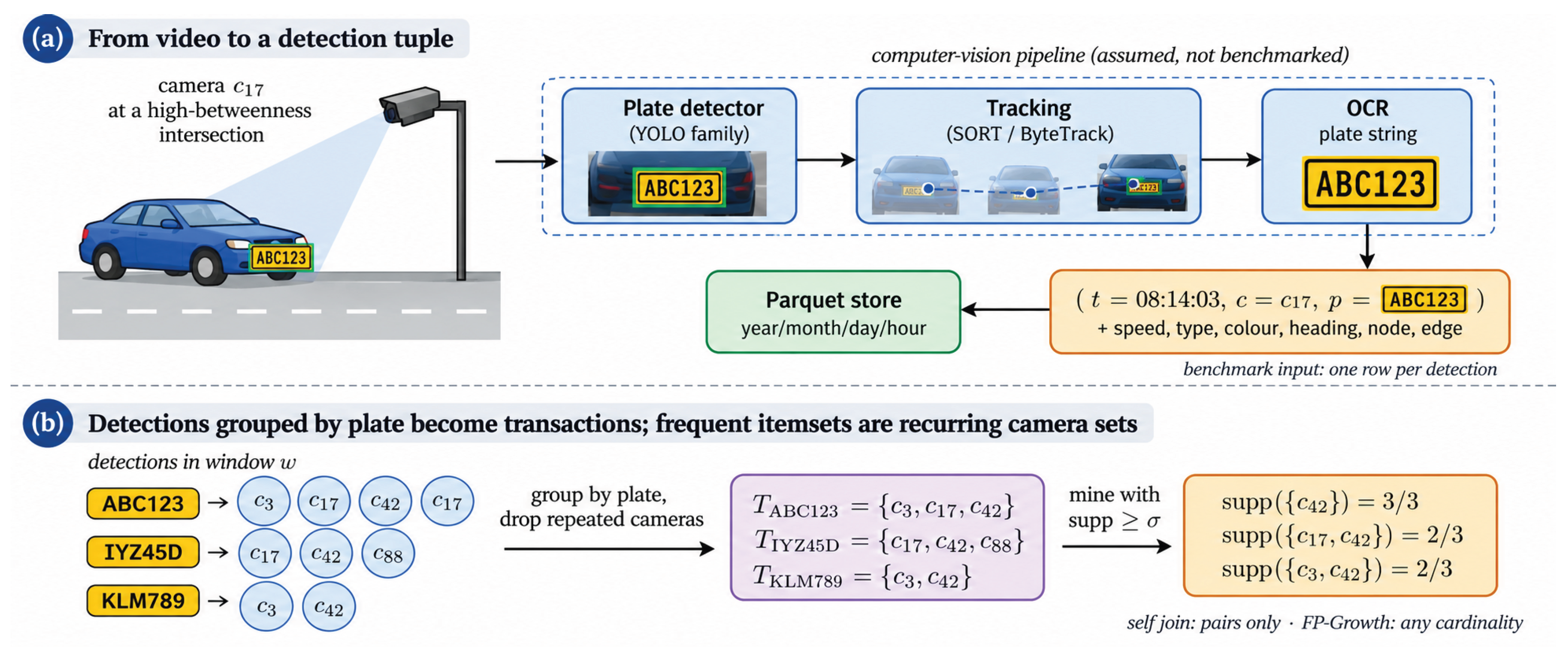
Figure 2.
Drivable road network of Pereira (largest strongly connected component, OpenStreetMap) and the 500 simulated camera locations, placed on the intersections of highest betweenness centrality. Marker colour and size are proportional to betweenness.
Figure 2.
Drivable road network of Pereira (largest strongly connected component, OpenStreetMap) and the 500 simulated camera locations, placed on the intersections of highest betweenness centrality. Marker colour and size are proportional to betweenness.
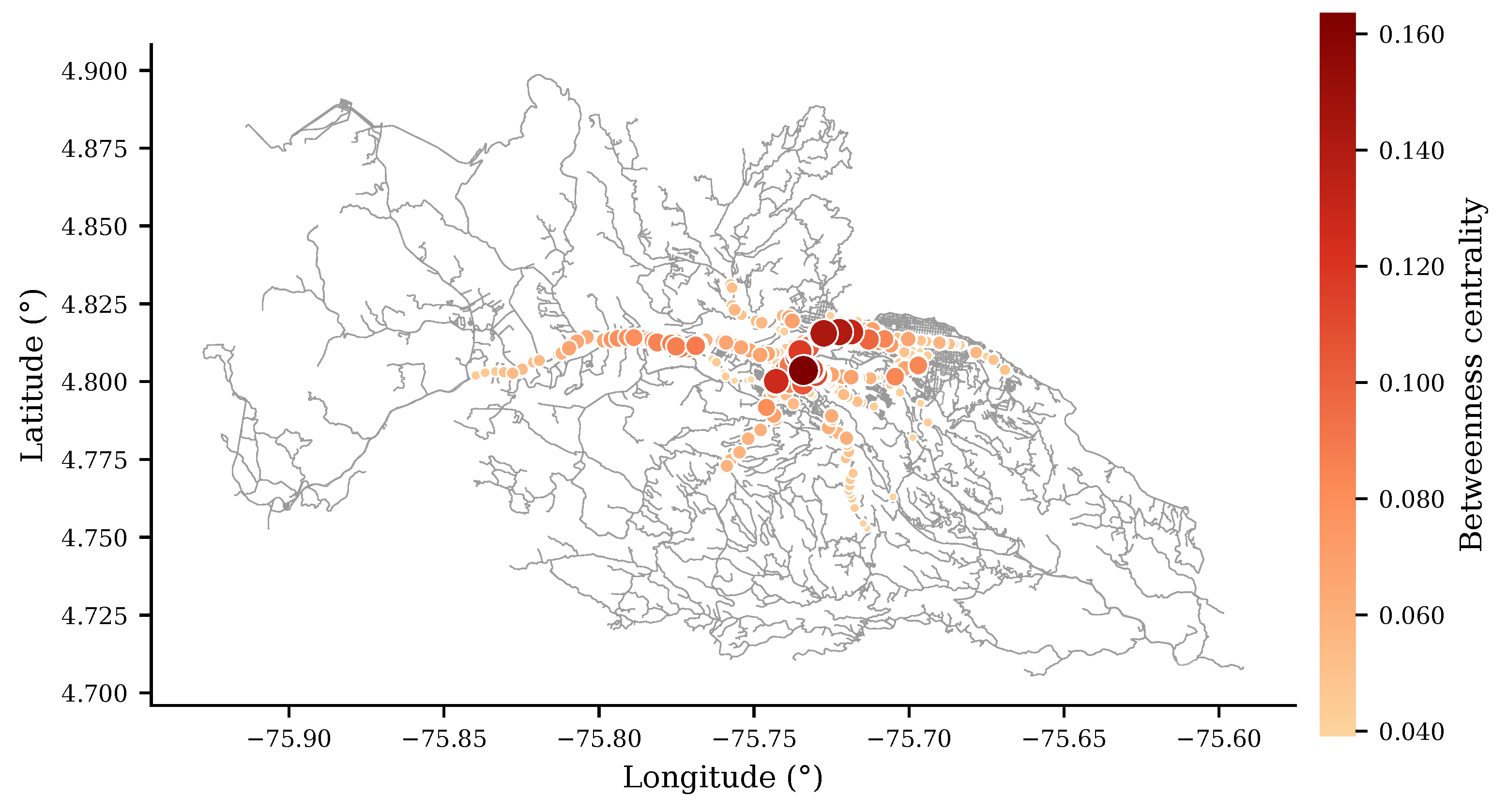
Figure 3.
End-to-end architecture of the experiment. The traffic simulation over the Pereira road graph produces a partitioned Parquet dataset; this is loaded into PostgreSQL through ETL and indexing, while Spark reads it directly. Five workloads are executed on both engines along a scalability ladder from 50 K to 15 M detections.
Figure 3.
End-to-end architecture of the experiment. The traffic simulation over the Pereira road graph produces a partitioned Parquet dataset; this is loaded into PostgreSQL through ETL and indexing, while Spark reads it directly. Five workloads are executed on both engines along a scalability ladder from 50 K to 15 M detections.
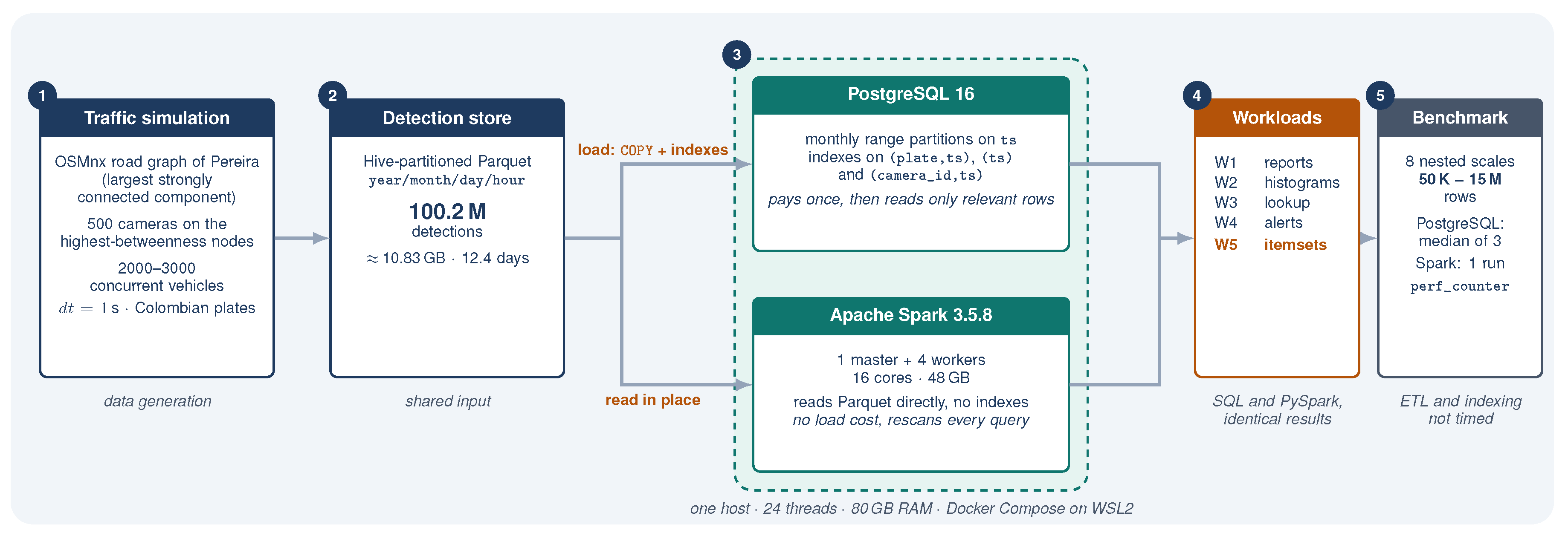
Figure 4.
Response time against number of rows on log–log axes for the five workloads. PostgreSQL (lower curve) dominates at every scale; the separation narrows drastically only in W5.
Figure 4.
Response time against number of rows on log–log axes for the five workloads. PostgreSQL (lower curve) dominates at every scale; the separation narrows drastically only in W5.
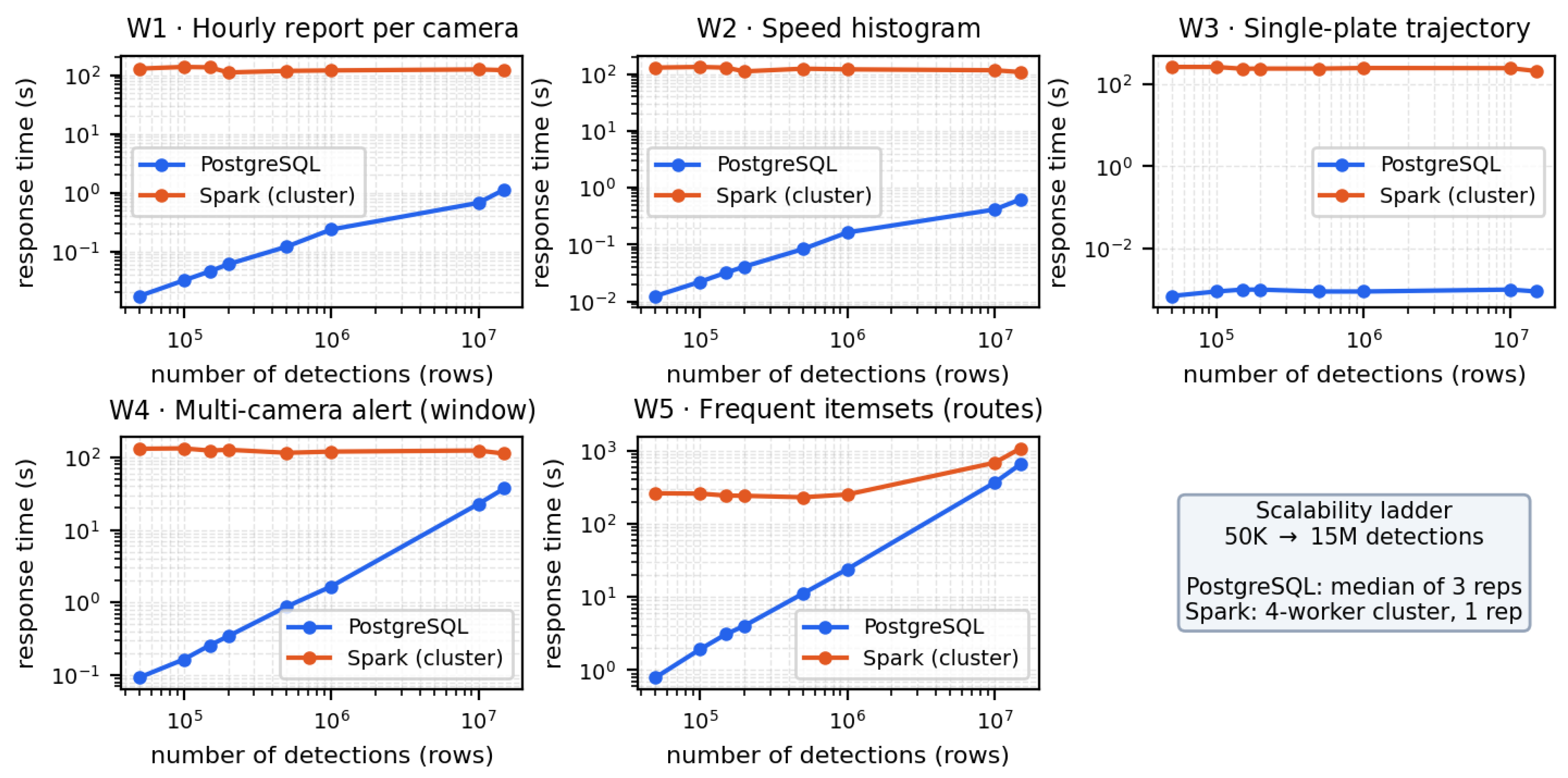
Figure 5.
Fixed overhead floor of Spark against the smooth scaling of PostgreSQL, on the report workload (W1, solid) and the mining workload (W5, dotted).
Figure 5.
Fixed overhead floor of Spark against the smooth scaling of PostgreSQL, on the report workload (W1, solid) and the mining workload (W5, dotted).
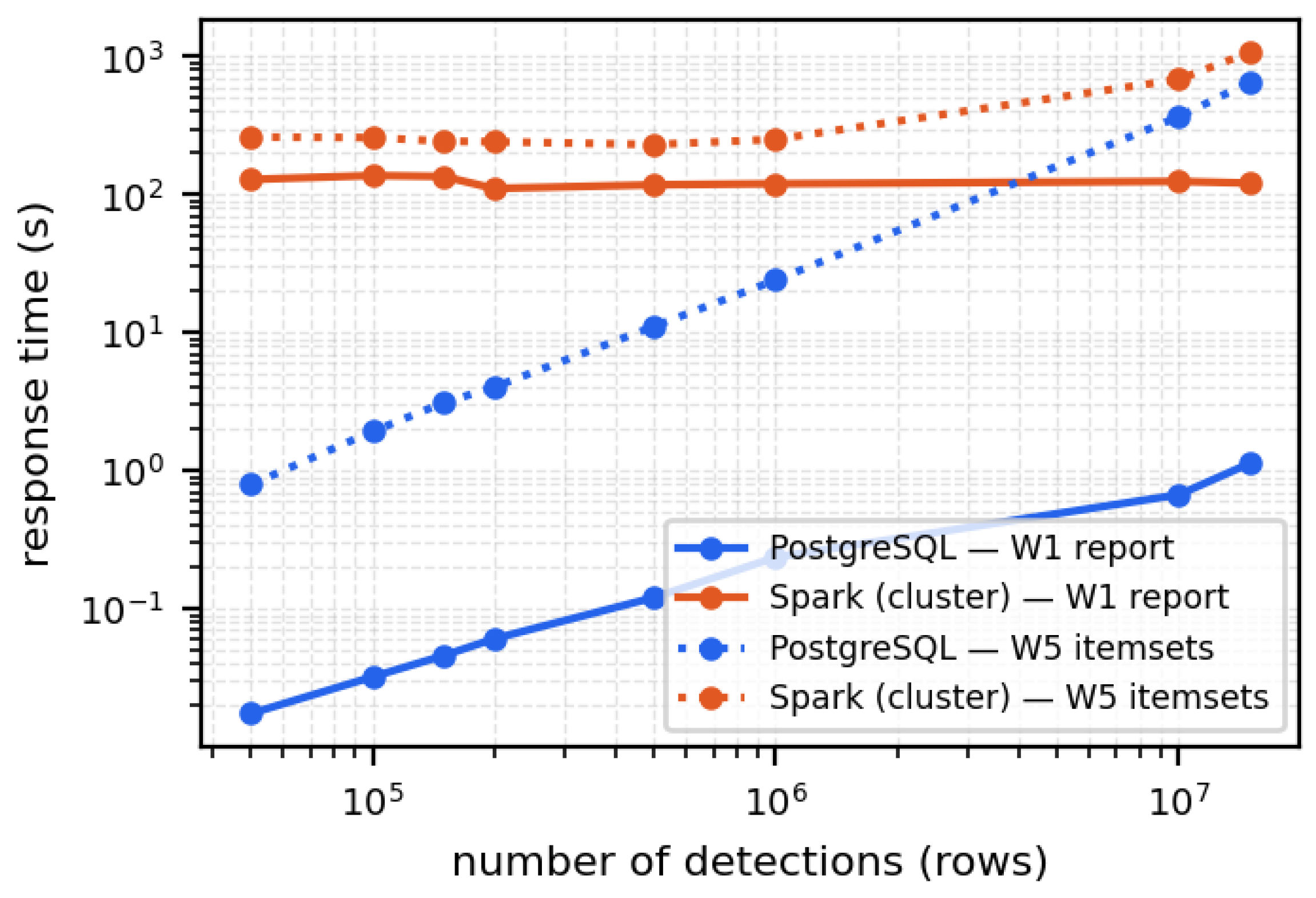
Figure 6.
Frequent itemset mining: response time against number of detections. The relational curve rises steeply from below one second while the distributed curve stays flat on its overhead floor until 1 M rows.
Figure 6.
Frequent itemset mining: response time against number of detections. The relational curve rises steeply from below one second while the distributed curve stays flat on its overhead floor until 1 M rows.
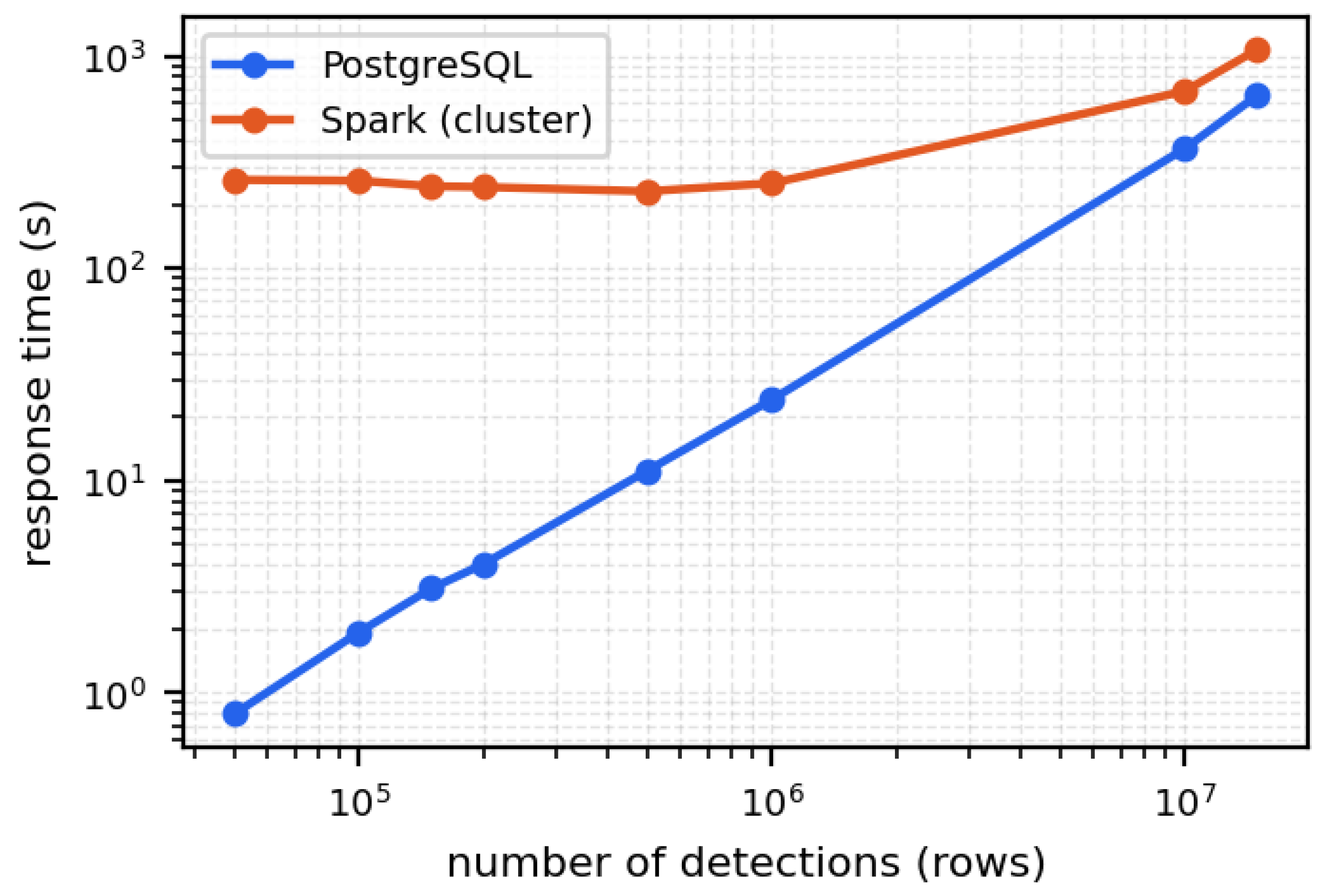
Figure 7.
Convergence in W5. Ratio of Spark time to PostgreSQL time against volume. The relational advantage erodes from to , indicating where the crossover would lie at larger scale.
Figure 7.
Convergence in W5. Ratio of Spark time to PostgreSQL time against volume. The relational advantage erodes from to , indicating where the crossover would lie at larger scale.
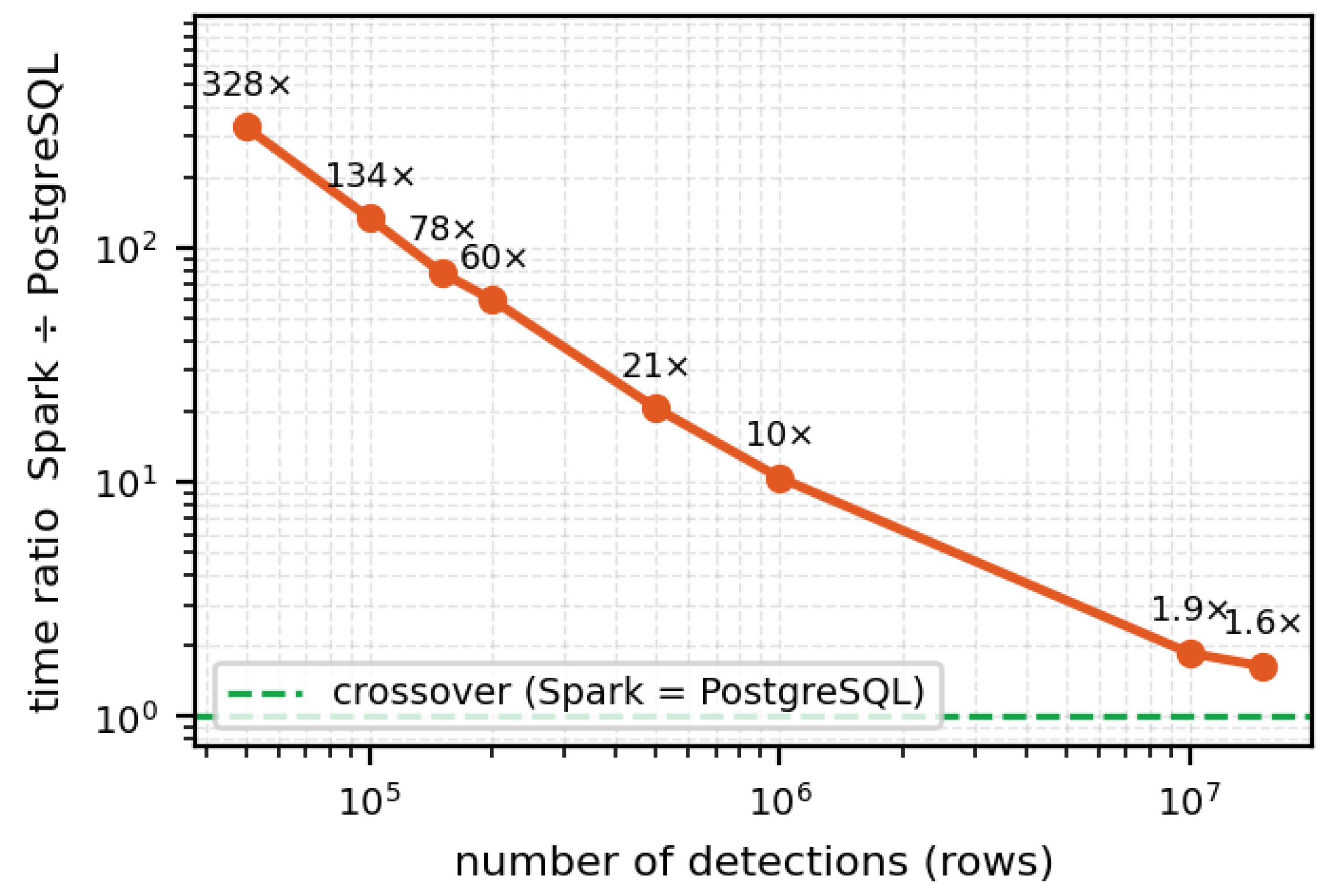

Table 1.
Statistics of the loaded dataset.
| Metric | Value |
|---|---|
| Rows (detections) | 100 225 733 |
| Distinct plates | 3 180 285 |
| Cameras | 500 |
| Temporal range | 12.41 days |
| Generation rate | M rows/day |
| Parquet size | GB |
| Vehicle mix | car 78.0% · motorcycle 18.0% · truck 4.0% |
Table 2.
Evaluated workloads.
| ID | Category | Question | SQL / PySpark implementation |
|---|---|---|---|
| W1 | Reports | Detections per camera and hour | GROUP BY / groupBy |
| W2 | Histograms | Speed histogram by vehicle type | WIDTH_BUCKET / floor |
| W3 | Lookup | Full trajectory of one plate | index seek / full scan |
| W4 | Alerts | Same plate at two cameras within 120 s | LEAD() / Window |
| W5 | Itemsets | Frequently co-visited camera sets | self join / FP-Growth |
Table 3.
Response time by workload, engine and scale (seconds). PostgreSQL: median of three repetitions; Spark: one repetition.
Table 3.
Response time by workload, engine and scale (seconds). PostgreSQL: median of three repetitions; Spark: one repetition.
| Workload | Engine | 50K | 100K | 150K | 200K | 500K | 1M | 10M | 15M |
|---|---|---|---|---|---|---|---|---|---|
| W1 | PostgreSQL | 0.0175 | 0.0322 | 0.0459 | 0.0607 | 0.1211 | 0.2365 | 0.6716 | 1.1 |
| Spark | 128.8 | 137.6 | 135.4 | 110.9 | 117.8 | 120.0 | 124.7 | 121.2 | |
| W2 | PostgreSQL | 0.0125 | 0.0222 | 0.0321 | 0.0410 | 0.0835 | 0.1633 | 0.4136 | 0.6249 |
| Spark | 129.3 | 132.8 | 129.2 | 111.0 | 123.7 | 120.5 | 116.2 | 107.8 | |
| W3 | PostgreSQL | 0.0007 | 0.0009 | 0.0010 | 0.0010 | 0.0009 | 0.0009 | 0.0010 | 0.0009 |
| Spark | 262.6 | 261.9 | 237.5 | 239.4 | 239.1 | 247.4 | 245.1 | 207.6 | |
| W4 | PostgreSQL | 0.0931 | 0.1649 | 0.2577 | 0.3440 | 0.8803 | 1.7 | 22.8 | 37.3 |
| Spark | 130.7 | 132.3 | 123.4 | 126.6 | 115.0 | 119.5 | 123.6 | 112.0 | |
| W5 | PostgreSQL | 0.7962 | 1.9 | 3.1 | 4.0 | 11.1 | 24.1 | 366.4 | 654.0 |
| Spark | 261.3 | 258.9 | 243.7 | 241.7 | 230.8 | 251.7 | 683.6 | 1074.4 |
Table 4.
Frequent itemset mining (W5): relational self join versus distributed FP-Growth. Ratio is Spark time over PostgreSQL time.
Table 4.
Frequent itemset mining (W5): relational self join versus distributed FP-Growth. Ratio is Spark time over PostgreSQL time.
| Scale | Rows | Self-join [s] | FP-Growth [s] | Ratio |
|---|---|---|---|---|
| s50K | 50K | 0.796 | 261.3 | 328× |
| s100K | 100K | 1.9 | 258.9 | 134× |
| s150K | 150K | 3.1 | 243.7 | 78× |
| s200K | 200K | 4.0 | 241.7 | 60× |
| s500K | 500K | 11.1 | 230.8 | 21× |
| s1M | 1.0M | 24.1 | 251.7 | 10× |
| s10M | 10.0M | 366.4 | 683.6 | 1.9× |
| s15M | 15.0M | 654.0 | 1074.4 | 1.6× |
Table 5.
Fitted growth exponents b in for W5. The values are two-point slopes.
| Engine | 50K–15M | 1M–15M | 10M–15M |
|---|---|---|---|
| PostgreSQL self join | 1.16 | 1.21 | 1.43 |
| Spark FP-Growth | — | 0.50 | 1.12 |
| Difference | — | 0.71 | 0.31 |
| Extrapolated crossover | — |
Disclaimer/Publisher’s Note: The statements, opinions and data contained in all publications are solely those of the individual author(s) and contributor(s) and not of MDPI and/or the editor(s). MDPI and/or the editor(s) disclaim responsibility for any injury to people or property resulting from any ideas, methods, instructions or products referred to in the content. |
© 2026 by the authors. Licensee MDPI, Basel, Switzerland. This article is an open access article distributed under the terms and conditions of the Creative Commons Attribution (CC BY) license (http://creativecommons.org/licenses/by/4.0/).
Copyright: This open access article is published under a Creative Commons CC BY 4.0 license, which permit the free download, distribution, and reuse, provided that the author and preprint are cited in any reuse.