

Submitted:
04 November 2026
Posted:
06 November 2026
You are already at the latest version
Abstract
The prevailing perception is that the transition to renewable energy will lead to a decrease in demand for hydrocarbons and petrochemicals. The present work empirically demonstrates that this common sense may be more imaginary than real: it finds evidence that renewable energy deployment may have a positive impact on hydrocarbons through its growing demand for petrochemicals. To obtain rigorous results, we employ state-of-the-art panel time-series methods that account for the main issues in panel data (e.g., cross-sectional dependence, non-stationarity, and heterogeneity) and provide insights for individual countries. Our key finding that renewables have a positive impact on petrochemical import demand is robust across various model specifications considered in the empirical analysis. Using the polymer intensities of the renewable energy systems and the estimated elasticities of demand for petrochemical imports, the global petrochemical polymer demand to meet projected renewable energy system penetration in a net-zero emissions scenario by 2050 was quantified to be in the range of 155 to 223 million metric tons (which translates to a growth in equivalent crude oil demand of 0.80 to 1.13 million barrels per day between 2025 and 2050), depending on the energy system design preferences. Import demand, which is an opportunity for petrochemical exporters, arising mainly from growth in the economies of India and China, accounts for between 67 and 96 million metric tons of polymer materials. The insights into policymaking in the petrochemical-importing economies are that their renewable transition will require more petrochemicals to be imported. The development of manufacturing capabilities for renewable energy technologies and high domestic petrochemical prices would further boost this import. Policymaking in petrochemical-exporting economies should consider that the findings may suggest opportunities to expand petrochemicals and related sectors, such as hydrocarbons.
Keywords:
renewables
; petrochemicals
; hydrocarbons
; imports
; developing economies
; panel time series analysis
1. Introduction
In 2015, all the United Nations (UN) member countries adopted 17 Sustainable Development Goals (SDGs) with 169 targets to be achieved by 2030 (https://sdgs.un.org/goals). Two of these goals constitute supportive steps towards implementing the Paris Agreement in practice. Energy transition from hydrocarbon to renewable sources is considered essential for achieving goal 7 – Affordable and Clean Energy, and goal 13 – Climate Action. Therefore, many studies have investigated various aspects of the renewable energy transition ranging from its economic growth effects to carbon emission features (see [1] and references therein).
Renewables as sources of energy are alternatives to fossil fuel sources, including hydrocarbons. Consequently, the renewable energy transition may negatively affect the hydrocarbon sector through two main channels. Firstly, through its effect on the heating and cooling (representing about half of the global final energy consumption) demand for fossil fuels (https://www.irena.org/Innovation-landscape-for-smart-electrification/Power-to-heat-and-cooling/Status). Secondly, the energy transition may reduce the transport sector’s demand for hydrocarbons. This sector is considered the main source of demand for crude oil, representing around 60% of the global consumption of crude oil [2]. Nevertheless, some forecasts indicate that this demand may decline by 40%, driven by an anticipated boom in electric vehicle adoption [3]. To this end, the prevailing view in the literature is that expansion in renewables would diminish hydrocarbon industry [4,5]. Such a view has formed (or largely contributed to) the prevailing common sense in the research community and policy making that the development of the renewable energy sector is negatively related to the hydrocarbon sector [6,7,8,9,10] (A downturn in the hydrocarbon sector would result in a decrease in petrochemicals due to the reduced availability of key feedstocks such as ethane, liquefied petroleum gases (LPG), naphtha, and methane. Additionally, due to complexity and other challenges alternative green feedstocks are not yet produced at sufficient levels to offset any decline in hydrocarbon-based feedstocks [11,12]).
The adverse effect of renewables on hydrocarbon described above is intuitive from the energy demand standpoint. From the non-energy use (e.g., non-combustion or feedstock) demand standpoint, however, it can be thought that the growing renewables may introduce opportunities for the hydrocarbon sector. Such opportunities have mostly materialized through the expected growth in petrochemicals such as plastic and rubber driven by the planned growth in the demand and thereby production of renewable energy equipment such as solar panels and wind turbines as projected by World Energy Outlook WEO [3] inter alia (Another opportunity might be the demand of the electric vehicle production for petrochemicals [19,20]. Increasing demand for electric vehicles is projected to accelerate demand for petrochemicals, such as rubber and plastic products (e.g. [12,18]). Since this channel does not directly link renewable energy to petrochemicals, it might be found to be a bit arguable. Hence, we do not consider it in this present work). Renewable energy industry relies heavily on products of petrochemicals [14,15]. Essential polymers, like ethylene and polyurethane, from petrochemicals, are crucial for manufacturing solar panels, which convert sunlight into energy. Similarly, the production of wind turbines necessitates materials such as steel, which is manufactured using powdered coal and natural gas. Additionally, various parts of the turbines, including engine houses, airfoils, and rotor blades, are crafted using resins sourced from petrochemical-based products, while oil-based lubricants are essential for the gearbox (e.g., see [12,14,15,16]). As IEA [12] and Bennett & Page [13] discuss, petrochemicals are rapidly becoming the largest driver of global oil demand for feedstock. Obviously, an expansion in the petrochemical sector will require more feedstock to be consumed, which is predominantly coming from the hydrocarbon sector, such as ethane, methane, naphtha, and liquefied petroleum gases (see projections in [12,17,18]) (The share of green feedstock such as biorefinery in total feedstock for petrochemical is quite small due to its given complexity and other challenges (e.g., see [11,12])). Thus, the emphasis of international energy agencies such as IEA and IRENA, through their future energy outlooks also suggest opportunities for substantial growth in the demand for petrochemical products.
To summarize the discussions above, on the one hand, many studies considered hydrocarbons and renewables as alternative sources to meet energy demand and concluded a negative relationship between the two. On the other hand, to date there is no dedicated applied research study estimating the impact of renewables, particularly solar and wind, industry on hydrocarbons particularly via demand for petrochemicals such as plastics and rubbers using realized/actual data, to the best of our knowledge (Note that Giannikopoulos et al. [8] simulated the impact of electrical vehicles on the US petrochemical sector. However, this research explores the petroleum refining industry and petrochemicals effects of vehicles, running on renewably generated electricity, but not the effect of renewable energy production or installed capacity. Additionally, that is a simulation analysis using optimization-based model not a behavioral analysis quantifying the impact by applying econometric method(s) to actual data). To this imbalanced end, the prevailing view in the research literature and (to some extent) in policymaking is that expansions in renewables negatively affect hydrocarbons, which should translate to a similar negative affect on petrochemicals which are derived from hydrocarbons.
This present work empirically demonstrates that the above-mentioned prevailing perception may be more imaginary than real by conducting a decent econometric analysis. This is the primary contribution of this study.
Dictated by data availability, we consider the top 7 developing economics in terms of renewable energy scale and investigate their petrochemicals imports (Our forthcoming study will examine the same topic for the developed countries). We consider petrochemicals because the renewable industry creates demand for petrochemicals such as plastics and rubber but not directly for hydrocarbons as discussed above. The advantage of considering petrochemicals’ import demand not aggregate demand is that derived policy insights could be useful for not only importing countries but also exporting ones.
In addition to its primary contribution above, this work possesses a few other merits. First, to the best of our knowledge, this is the first study to numerically assess the impact of renewables on petrochemical imports. The renewable energy transition is a phenomenon that every industry including petrochemicals and hydrocarbons should assess for its potential effects. Second, we base our analysis on the theory of import demand and expand upon it by incorporating renewable installed capacity. Such an extension aligns with previous studies on import demand (e.g. [21,22,23,24,25]). Furthermore, it can be characterized as a combination of theory-driven and data-driven approaches – a practice widely employed and endorsed for applied research by leading scholars (see, for example [26,27,28,29,30,31,32]). Third, to obtain sound results and suggest grounded policy insights, we address the main issues of the panel data, namely cross-sectional dependency, non-stationarity, and heterogeneity using the state-of-the-art panel time-series methods. Fourth, many panel studies conducted pooled analysis and ended up suggesting the same policy recommendations for all countries in the panel. Such ‘one size fits all’ type recommendations ignore country specificities and hence, would not be quite useful for individual countries’ policymaking. To avoid this and being able to suggest country-specific policy recommendations, we estimate petrochemicals import demand function for each individual country separately.
This study is organized as follows. Section 2 presents the theoretical framework and empirical model of the study. Data is discussed in Section 3. Section 4 describes empirical analysis strategy and econometric methodology. The results of the empirical analysis are documented in Section 5 and their discussion is given in Section 6. Section 7 concludes the study with some policy insights.
2. Theoretical Framework and Empirical Model
The theoretical underpinning of our study is the international trade theories developed in Leamer and Stern [33], Goldstein and Khan [34], Rose and Yellen [35] and Rose [36]. According to these theories, in the framework of the imperfect substitutes model of a Marshallian demand, total quantity of imports demanded by a country is related to its real income (or real expenditure or any other scale variable which captures domestic demand conditions) and relative prices. This is the standard form of the import demand function and widely used in empirical studies (e.g., see [21,37]). It can be expressed with the following un-specified function as:
Where, M and Y are demand for goods to be imported and income of the importing country, respectively. PR is the relative prices. It can be defined as . That is, the ratio of the prices of imported goods in the international markets (PF) to the prices of imported goods in domestic markets (PD), both expressed in the same currency, for example in the US$, respectively. Usually, PDis in local currency multiplied by the exchange rate of say US$ against the local currency. This is to express the domestic price in US$, so both prices will be in the same currency, i.e., US$.
As discussed above, this research is interested in exploring the role of renewable energy in the import demand for petrochemicals, to come up with policy insights that are useful for both importers and exporters of petrochemicals. Therefore, we include our variable of interest, that is, renewable energy (RE) in the equation of petrochemicals import demand (MP). Note that extending a standard import function with a variable of interest is widely considered in literature. For example, the standard import demand specification is extended by income inequality in Adam et al. [21] and Konstantakopoulou [22], by transitory income in Doroodian [23], by foreign exchange reserves in Hosen [24] and by expenditure components in Chani et al. [25]. Moreover, extending theoretical framework (e.g., equation (2.1)) with the variable of interest, that is, RE can be considered as the combination of theory-driven approach with data-driven approach, which is widely used and also recommended for empirical studies by seminal scholars (see e.g. [26,27,28,29,30,31,32]). Such an extended equation in the case of the panel data and econometrically estimable form can be expressed as follows:
where, ln denotes the natural logarithm, εit denotes the error term. α0 is the constant term, while α1 − α3 are the elasticities of petrochemical imports with respect to income, relative prices, and renewable energy, respectively. α0 − α3 coefficients are to be estimated econometrically. i and t indicate sections/panel members and time, respectively. i = 1, 2,…N and t = 1, 2,…T. N and T are the number of panel members and time series observations, respectively.
Theoretically, one should expect, α1 > 0 meaning that demand for import increases when the income of the importing country rises. α2 < 0, which suggests that a country’s demand for imports should decrease if the international market prices of petrochemicals are higher than the domestic prices, both expressed in the same currency, e.g., US$. Conceptually, we expect α3 > 0 based on our discussion above.
The coefficients in equation (2.2) are the pooled coefficients. In other words, they are the same for each member/section of the panel. This is the traditional panel methodology. However, one of the merits of our study, as we discussed above, is that we will use modern panel methodology, which allows us to estimate the coefficients of a given relationship for each panel member/section. This is extremely important as it enables us to provide section/member-specific policy recommendations, which cannot be derived from the application of the traditional panel methodology. Thus, our empirical model of petrochemical imports in the case of section/member-specific coefficients can be expressed as below:
3. Data
In the ideal case, we should consider renewable manufacturing, mainly solar panels and wind turbines, in the analysis. The available data show that the top countries of solar panel manufacturing in 2021 are China, Vietnam, Malaysia, South Korea, United States, India, Thailand, Taiwan, Europe, Japan, Singapore, and Canada; with China having the share of 75% out of 100% (https://www.statista.com/statistics/668749/regional-distribution-of-solar-pv-module-manufacturing/#:~:text=China dominates the solar industry, leader in installed PV capacity). Regarding wind turbines, 9 out of the top 15 manufacturer in 2022 are located in China while the rest 6 are in Germany, Denmark, Spain, and France (https://www.blackridgeresearch.com/blog/top-wind-turbine-manufacturers-makers-companies-suppliers). The above are the only data available on manufacturing of solar panels and wind turbines. Obviously, they are not sufficient for our econometric analysis because we need data by country and year, and that is not available. Therefore, we adopt data on the installed capacity of solar and wind power systems, which are the closest representation of the solar panels and wind turbines manufacturing. We take this position because one can reasonably think that manufacturers of these renewable energy systems are more likely to consider the domestic market first before exploring export opportunities to other countries, considering the pressing climate change related to local and international commitments, policies, agreements, and measures, in addition to energy security issues.
To this end, we considered the top 7 developing countries in terms of the share of installed solar and wind power generation capacities over the last 10 years, using data from the Statistical Review of World Energy database 2023 release. They are ranked as China, India, Brazil, Turkey, Mexico, Chile, and Thailand (Initially we had also Poland, Romania, and Czechia in our sample, and an empirical analysis was conducted considering all these 10 countries in the previous version of this paper. In the current version of the paper, we have excluded these three countries following a referee’s suggestion expressing that they are classified as developed countries for the second half of the sample (see the United Nations World Economic Situation and Prospects reports)).
The time dimension of our sample covers 1996-2022. The starting year of the sample is dictated by the availability of the data on renewable installed capacity for solar and wind energy systems, which go back as far as 1996. Table 1 below documents the variables through their definition, measurement, and source.
Table 2 below presents essential descriptive statistics for the variables of petrochemicals import and the installed capacity of solar and wind power systems in the countries under consideration.
Figure 1 below illustrates the same variables for each country over the time sample of 1996-2022.
Figure 1.
Petrochemical imports (left axis, blue line) and renewable energy installed capacity (right axis, orange line).
Figure 1.
Petrochemical imports (left axis, blue line) and renewable energy installed capacity (right axis, orange line).
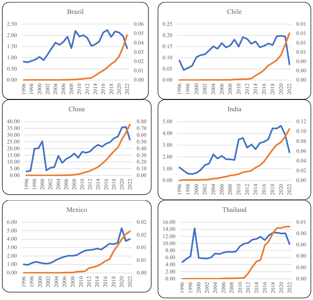
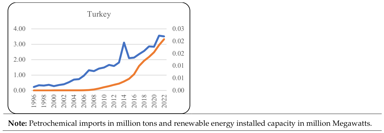
One of the noteworthy observations from the figure is that installed renewable capacity increased significantly since 2012 or so in each country. Another observation is that petrochemical imports have been increasing over time, although they declined in 2022 in almost every country. This decline was mainly due to low growth in the selected economies and the Russia-Ukraine conflict [38,39]. Lastly, installed renewable capacities are smooth over time with less variation whereas petrochemical imports demonstrate more variation in the countries under consideration. Even, the latter variable has spikes in some countries, such as China, Mexico, Thailand, and Turkey.
4. Empirical Analysis Strategy and Methodology
Figure 2 below illustrates our strategy for empirical analysis while Table 3 presents panel methods that can be potentially considered depending upon the conclusion of the strategy.
Figure 2.
Empirical analysis strategy. Source: Re-produced from Hasanov et al. [40]. Note. CD=Cross-sectional dependence; UR=Unit Root; FG=First Generation; SG=Second Generation; LR=Long-run; SR=Short-run.
Figure 2.
Empirical analysis strategy. Source: Re-produced from Hasanov et al. [40]. Note. CD=Cross-sectional dependence; UR=Unit Root; FG=First Generation; SG=Second Generation; LR=Long-run; SR=Short-run.
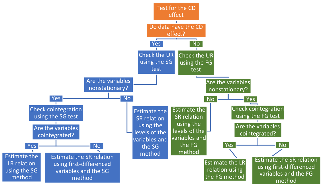
A conclusion from Figure 2 is that one should use second-generation panel methods to test unit root, cointegration and to estimate the long-run relationship between petrochemical imports and explanatory variables if the data demonstrate cross-sectional dependency (CD), which will be decided based on the CD test results.
In the case of two explanatory variables (regressors), the panel version of the Autoregressive Distributed Lags (ARDL) assuming heterogeneity of all coefficients, i.e., the Mean Group (MG) method due to Pesaran and Smith [49], in the level form of the variables, can be written as below:
where Y is the dependent variable; X and Z are the regressors; i=1,2,…,N and t=1,2,…,T denote panel cross/member and time, respectively; k changes from unity to p for the dependent variable and from zero to p for explanatory variables; p and q are the maximum numbers of lags for the dependent and explanatory variables, respectively.
where ft is an m × 1 vector of unobserved common factors, Γi is an m × k vector of factor loadings and εit is the individual-specific, i.e., idiosyncratic errors.
To approximate unobserved common factors, , the MG in equation (4.1) can be augmented by cross sectional averages (CSAs) of the variables, as discussed in Pesaran [50], Chudik and Pesaran [51] inter alia.
Where ; ; .
Note that contemporaneous and lagged values of CSAs of the variables can be used for this purpose. Pesaran [46] discusses that usually one lag of the level and contemporaneous value of the first difference of CSAs are sufficient to filter out the effects of the unobserved common factors, . It further notes that the lag orders can be high if N, i.e., the number of cross-sections are large. Thus, the MG with CSAs of the variables can be expressed in the following equation:
where α1i, α2i, and α3i are the coefficients to be estimated econometrically. εit is the individual-specific, that is, idiosyncratic error terms. p1 − p6 are the lag orders and not necessarily equal to each other.
The long-run coefficients for X and Z can be calculated from (4.2) using the formulas below:
Thus, the long run equation of Y can be expressed as follows:
5. Results of the Empirical Analysis
This section provides the results of the econometric estimations and testing. The first part of the section presents the results of cross-sectional dependence, unit root tests, and cointegration test, while the long-run estimations results are given in the second part.
We used recently developed tests of Pesaran [52], Fan et al. [53], and Pesaran and Xie [54] to check whether the variables have the issue of cross-sectional dependence (CD). The test results are documented in Table 4.
For mp, reic, and y, all three tests performed reject the null hypothesis of weak CD effect in favor of the alternative hypothesis of strong CD effect. For pr only two out of three tests reject the null hypothesis. In overall, the test results suggest that the variables, particularly our main variables of interest, i.e., mp and reic, are cross sectionally dependent. Statistically, the key message from these results is that for checking unit root and cointegration properties of the variables, as well as for estimating mp equation in (2.4), we need to use methods that account for CD effect.
Table 5 documents the results of the panel unit root tests developed by Pesaran [46], which is the second-generation test accounting for CD effect.
The table indicates that the cross-sectionally augmented Im-Pesaran-Shin (CIPS) test by Pesaran [46] decisively suggests unit root process in the form of integrated order of one, i.e., I(1) for all the variables except for pr. This is because none of the sample Z statistics in the table from the test of the levels of the variables is greater than the critical values in absolute terms (see the second column). Hence, the null hypothesis of unit root cannot be rejected for all variables. However, the sample Z statistics are greater than the critical values from the test of the first difference of the levels, which lead to the rejection of the null hypothesis, except for pr (see the third column). These results are satisfactory enough to conclude that the log level of the variables, i.e., mp, reic, and y are unit root processes. Regarding pr, we tested the second difference of it, that is, d2_pr. The test sample statistic is hugely greater than the critical value. This suggests stationarity of the second difference of pr meaning that pr is second order difference stationary variable, i.e., I(2) process. Thus, the implication of the unit root test results is that in the long-run analysis, such as cointegration test and estimation, mp, reic, y, and first difference of pr, d_pr, should be used. While in the short-run analysis, the first difference of the other variables and the second difference of pr, that is, d_mp, d_reic, d_y, and d2_pr should be considered.
Since we found the variables to be non-stationary in their levels, it gives a good reason to think that they may establish a long-run relationship. If it is the case, then we will be interested in estimating numerical parameters of this long-run relationship for mp. To check whether variables establish the long-run relationship, we use Westerlund [47] cointegration test accounting for the CD effect. The results are recorded in Table 6.
The Westerlund [47] test statistics, Ga, Pt and Pa, with bootstrapping confirms the existence of cointegration among the variables. It is well-known that Westerlund [47] test statistics under-reject the null hypothesis if data span is small like our case here, as he discusses it in Westerlund [47]. Given that, it is very promising that three out of four test statistics indicate a co-integration among the variables even though we have a small sample span. In conclusion, the variables under consideration, i.e., mp, reic, y, and d_pr are cointegrated. Put differently, mp may establish a long run relationship with the explanatory variables considered.
As mentioned above, finding cointegrating relation among the variables gives ground to estimate equation (2.3) for mp, which would provide us with the long-run elasticities of it with respect to the explanatory variables. We used the CCE MG as a method for estimating the long-run elasticities. The impact of renewable energy on petrochemicals import is our main interest in this study. Therefore, we report its impact both for a pool of countries (in Table 7) and for each individual country in the pool (in Table 8). The effects of the relative prices and income, on the other hand, are only reported at the pooled level.
In deciding on the statistical significance of the estimated coefficients we consider till 16%. This is because we have a small number of observations. Note that considering 16% of significance level is in line with the empirical studies conducted by seminal econometricians, such as David Hendry, James Stock and Lutz Kilian (see [55,56,57,58]). Note that even if we adopt statistical significance till 16%, our main variable of interest, reicit is statistically significant at the 5% level. Moreover, the relative prices variable is statistically significant at the 10% level with the theoretically expected negative sign. The Income variable also takes theoretically expected sign, which is positive, although it is not statistically significant. If we exclude it from the estimation, we still get positive and more statistically significant impact of reicit our variable of interest, being 0.173 with the probability of 0.008. Constant is statistically significant at 16%. Even if it is statistically insignificant, we would not exclude it from the estimation because it is hard to assume that the initial level of mpit is zero. Thus, we prefer to stick with the estimation results of equation (2.3) as it retains theoretically articulated factors namely income and relative prices, in which our variable of interest is statistically significant with the expected positive sign. Table 8 presents the country specific long-run elasticities of petrochemicals import with respect to renewable energy installed capacity estimated from equation (2.3).
The main takeaway from the table is that the impact of reict on mpt is positive for all countries at different levels of statistical significance, none of them is negative.
For Brazil, the impact of reict on mpt initially was negative 0.060 with the p-value of 0.788 from the standard PMG estimation. A s it is discussed in the data section, Brazil is ranked number third in terms of installed capacities of solar panels and wind turbines. In addition, the graph for Brazil in Figure 1 illustrates that reict and mpt co-move with upwarding trend over time. Hence, obtaining a negative coefficient would cast some doubt. Thus, we further investigate Brazil to make sure that the obtained estimate is an accurate representation of the impact of reict on mpt and is not the result of data issue. In this regard, one should have a good reason to suspect that the estimation results for Brazil might be caused by the huge drops in the time trajectory of mpt in 2008 and 2022. Numerically speaking, mpt dropped as largely as 31% and 32% in 2008 and 2022 relative to the previous years, respectively. This drops in the mpt series were not captured in the panel estimation. Therefore, we re-estimated the ARDL equation for Brazil by accounting for these huge drops using two dummy variables. All the post-estimation and cointegration test results are acceptable (The ARDL(1,1,0,0) was selected by the Akaike information criterion from the ARDL(1,1,1,1) for the mpt equation with the regressors d_prit, yit, and reicit. The null hypotheses of no autocorrelation, no serial correlation, normality, homoscedasticity cannot be rejected at the conventional significance levels. Additionally, the Bounds test indicates cointegration among the variables, as the sample F-value of 8.74 is higher than the critical upper bound F-value of 5.966 in the case of 30 observations and intercept is included in the long-run equation.). The estimation yields the long-run elasticity of mpt with respect to d_prit, yit, and reicit to be -0.167, 2.566, and 0.178 with the probability values of 0.042, 0.000, and 0.000 i.e., all three being statistically significant. If we replace these elasticities above with the ones estimated from the standard PMG for Brazil, then the panel elasticities for the pool of seven countries reported in Table 7 will change to -0.858, 1.043, and 0.229 for d_prit, yit, and reicit , respectively.
Robustness Check for the Estimated Positive Impact of Renewables on Petrochemicals
We estimated a positive impact of renewables on demand for petrochemicals’ import from the equation (2.3) as reported in Table 7. Econometrically, this is a multiple regression, in which an estimation of the coefficient of a regressor involves variance and covariance of the regressors in the equation as well ([59], Chapter 7). Given that income elasticity of the petrochemicals’ import demand was statistically insignificant in the estimation of equation (2.3.), one can be interested in exploring what would happen to the estimate of renewables elasticity if the equation were estimated without income variable in it. In other words, whether the impact of renewables on petrochemicals’ import demand will still preserve its robustness by getting positive and statistically significant coefficient. As a further robustness, one can challenge the renewables’ impact by estimating various modifications of equation (2.3). To this end, we considered all possible relevant reduced forms of equation (2.3) by excluding regressors. This yielded the following four specifications: (i) without income; (ii) without relative prices; (iii) without income and relative prices; (iv) without renewables. (By relevant we mean specifications, which include renewables and a standard import demand specification including income and relative prices only. Table 9 reports the estimation results.
The key takeaway from the table, with respect to our focus, is that renewables consistently exhibit positive and statistically significant elasticities across all three specifications, from Model 1 to Model 3. Two other notable findings are as follows: First, none of the estimations from these four specifications outperform theoretically and statistically those from equation (2.3) in Table 8, which was our preferred specification. This finding reaffirms our choice even though the income elasticity is statistically insignificant. Second, the standard import demand model, that is, equation (2.3) without renewables in Model 4 does not yield any superior results compared to our preferred specification, i.e., equation (2.3), where renewables are included. This suggests that augmenting equation (2.1), that is, the theoretical import demand model with renewables was a reasonable strategy, which is in line with suggestions of combining theory-driven and data-driven approaches as discussed in Section 2.
In summary, the analysis conducted here demonstrates that the positive impact of renewables on petrochemicals remains robust if various specifications are considered.
6. Discussion of the Results
According to Table 4, the variables under consideration are correlated across the countries in our sample. Such a cross-country correlation or dependence of a given variable can happen due to the existence of factors that are common for these countries. These factors might be due to globalization, international spillover effect of technologies and efficiency measures as developing economies try to catch up with advanced economies, international economic linkages including trade, capital/investment flows, prices at the global markets, shocks and recessions that have a global coverage, climate change related policies and measures (see discussions in Bai et al. [60]; Pesaran [61], Chapter 29; Baltagi and Pesaran [62]).
The unit root process, i.e., non-stationarity, suggests that the variables are continuously drifting over time and do not return to their previous average as the average value itself changes. Any disturbance or shock to such drifting variables can have a lasting impact. Predicting future values of these variables is challenging due to the changing average and the permanent effects of shocks. For prediction purposes, it is advisable to use a stationary transformation of the variables to overcome this issue. Stationary series have consistent mean, variance, and covariance over time, and they fluctuate around their mean values. These stationary series are known as mean-reverting processes because they tend to revert to their mean values.
From the cointegration test results, we found that imports of petrochemicals have a long-run relationship with renewable energy, relative prices, and income. In other words, petrochemical imports share a common trend with these factors, and they move together, establishing an equilibrium relationship in the long run. Another interpretation of cointegration is that the relationship among (the logarithmic levels of) the variables is not a chance occurrence, i.e., spurious, rather it aligns with economic thinking. Consequently, the estimated long-run coefficients can be used for analysis and projections.
We estimated the long-run impacts of renewable energy, relative prices, and income on petrochemicals import for the pool of countries as well as for each country. Since renewable energy is our main variable of interest in this study, we discuss its impact on petrochemical imports both for a pool of countries and for each individual country, whereas the impacts of the relative prices and income are discussed at the pooled level only.
Table 7 shows that for the panel of the countries, a 1% increase in renewable energy installed capacity increases petrochemical imports by 0.2% in the long run keeping other factors unchanged. Turning to the country specific results reported in Table 8, the first observation is that the elasticity of petrochemical imports with respect to renewable energy installed capacity is expectedly positive for all seven countries in our sample. This finding shows that expansion in the renewable energy installed capacity can lead to more imports of petrochemicals in 100% of the entire sample under consideration.
It is conceptually/theoretically expected that an increase in renewable installed capacity requires an increase in its manufacturing, which requires more consumption of petrochemicals such as rubber and plastics. In particular, the demand for (reinforced) plastic materials, resin, polymer matrix would increase to produce encapsulant, back-sheet, wind turbine blades (e.g. [63]). Such plastics, which are sourced from chemical and petrochemical substances, can also play a role in the next round of cost reductions in renewable energy generation. For example, in the wind energy sector, light-weight plastic-based materials can help address the challenges of making longer turbine blades, thereby increasing generation efficiency. Innovative materials can also help increase the durability of wind turbines, thus reducing the cost of maintenance. This is especially beneficial in harsh environments, such as those offshore or similar remote locations (see e.g. [12]).
There are a number of processing pathways for non-combustion oil demand as feedstock for petrochemical industry. The most common and existing commercial pathway is via oil products from refineries such as naphtha and liquefied petroleum gas (LPG), and these account for about 17% of current global oil demand. With ethane feedstock from other hydrocarbon liquids (natural gas liquids) included, the number rises to about 22% of the oil demand [64]. Under various IEA scenarios for 2050, global oil demand arising from petrochemical production is projected to be in the range of 50% and 80% of total oil demand by 2050 [64]. The majority of this demand is expected to emanate from developing and emerging economies where factors such as population growth, rising standard of living, and industrialization would be the drivers.
Moreover, the IEA’s projected scenarios for sectoral energy consumption by 2040 pointed out that non-combustion demand for oil – i.e., as a feedstock for petrochemicals and chemicals production – is expected to lead the final energy consumption growth, as petrochemical sector’s demand for feedstocks is forecasted to rise by 41% and 29%, according to the Stated Policies (STEP) and Sustainable Development (SD) scenarios, respectively [18].
Thus, as calls for combating climate change propels global energy transition towards higher renewable energy penetration major expansions of the global petrochemicals sector are envisaged.
The estimation results also show that, the size of the elasticity varies from the minimum of 0.021 in Thailand to the maximum of 0.610 in China. This reveals differences in the response of petrochemical imports to the renewable energy installed capacity in the countries considered driven by their specificities, although all of them are developing nations. Such specificities include the degree of diversity of applications of petrochemical products in the country, among others. Indeed, one would not expect the response of say India to be the same as that of Chile.
Moreover, none of the positive elasticities are greater than unity, that is, they are inelastic, meaning that an increase in the renewable energy installed capacity causes less than the same magnitude of increase in the imports of petrochemicals in the countries considered. Furthermore, the elasticities are statistically significant at the 16% level or higher for 4 of 7 countries, that is, China, Brazil, Mexico, and Turkey. While they are not statistically significant in Chile, India, and Thailand. This might be interpreted that in China, Brazil, Mexico, and Turkey the level of the development of the renewable energy installed capacity is high enough to significantly influence imports of petrochemicals. On the contrary, the level is not high enough in other countries to make a significant impact.
Table 7 further reports that for the panel of the countries, 1.0% fall in petrochemical imports is caused by 1% increase in the relative prices of international to domestic in the long run. The negative relationship found here is in line with demand theories, including those for imports. When it comes to the magnitude of the impact, the estimated opposite one-to-one relationship between petrochemical imports and the relative prices is due to country characteristics. It shows that these seven countries’ petrochemical imports are quite sensitive to changes in petrochemical prices in the domestic and international markets.
Lastly, Table 7 documents that a 1.0% increase in the income of the countries considered, measured by manufacturing value added, leads to a 0.7% increase in their demand for petrochemical imports. This finding is consistent with demand theories, although it is not statistically significant at the conventional levels. The statistically insignificant income effect found might imply that petrochemical products are a kind of necessary good for the manufacturing sectors of these countries. Hence, regardless of the level of income, these goods have to be imported to materialize the production process. Such an explanation is supported by previous studies. For example, Guo et al. [19] found that electrical vehicle production increases demand for petrochemicals and hence, oil imports.
Moreover, our finding of the positive impact of the manufacturing sector on (imported) demand for petrochemicals (i.e., plastics and rubber) is also consistent with the findings of other previous studies. They find that a higher demand for petrochemical products such as plastics and rubber is created by manufacturing of automobiles, electrical and electronics [8,19], healthcare [12], textiles [65], food processing [66], and packaging [67]. As IEA [12], among others discusses, petrochemicals are the raw materials/intermediate goods for many manufacturing sectors including but not limited to fertilizers, packaging, food, pharmaceuticals, and automobiles. Thus, the overall demand for petrochemicals is derived from demand for these manufacturing sectors’ output. Therefore, the structure of economies can considerably affect demand for petrochemicals. This is especially true for developing and less-developed economies given that structural transformations in these economies are towards industrialization.
Popular Perceptions Regarding Petrochemicals: Insights from a Survey
Our first goal was to assess the general public’s perceptions regarding the relationship between climate change mitigation and petrochemicals. To do this, we conducted a survey based on the UN’s “People’s Climate Vote,” a 2021 UN survey in which 1.2 million people from over 50 countries participated. We made this decision for two reasons. The first was to economize on the survey design effort in light of how well-designed the UN survey was. The second was to leverage the UN survey’s policy tone: the survey sought to understand global public opinion on climate change with the aim of informing and encouraging more ambitious climate action by governments, businesses, and international organizations. This matched our desire to gauge the sorts of opinions that might be used to influence policy. A full description of the methods we used is included in the Methods section of this paper.
The original UN survey’s questions were structured to assess people’s personal experiences with climate change and their level of concern, with specific inquiries about how the issue impacts their daily lives and if they believe it constitutes a global emergency. The survey also explored public support for a wide range of policy priorities, in addition to asking whether countries should set aside geopolitical differences to work together on climate action. Notably, it included no questions about petrochemicals. However, we added two petrochemicals questions that were loose analogues to equivalent questions relating to fossil fuels:
Original question 1: How quickly should your country replace coal, oil, and gas with renewable energy, such as power from the wind or sun? (Very quickly / Somewhat quickly / Slowly / Not at all / Don’t know).
New question 1: Should your country increase or decrease its demand for petrochemicals such as ethylene, polyurethane, resins, and oil-based lubricants? (Increase / Decrease / About the same as now / Don’t know).
Original question 2: Should countries work together on climate change even if they disagree on other issues, such as trade or security? (Yes, they should work together despite their disagreements / No, they should work separately / It doesn’t matter, no country should work on climate change / Don't know).
New question 2: Should countries work together to decrease global production of petrochemicals such as ethylene, polyurethane, resins, and oil-based lubricants? (Yes / No / Don’t know).
We also added two novel questions that were not inspired by (or modified versions of) ones from the UN survey, with the goal of more directly gauging people’s opinions about the net impact of fossil fuels and petrochemicals.
New question 3: On balance, what role do you think that fossil fuels (coal, oil, natural gas) can play in your country in the transition toward clean energy? (Positive / Negative / Don’t know).
New question 4: On balance, what role do you think that petrochemicals (ethylene, polyurethane, resins, and oil-based lubricants, etc.) can play in your country in the transition toward clean energy? (Positive / Negative / Don’t know).
Approximately 2,000 participants completed the survey during the month of August 2025: 500 from each of the UK and the US, with the remaining 1,000 coming from four of the world’s most aggressive investors in renewable energy capacity (Brazil, Chile, India, and Mexico). The main findings are shown in Figures 1–3.
Figure 1.
Preferences regarding home country demand for petrochemicals. Should your country increase or decrease its demand for petrochemicals such as ethylene, polyurethane, resins, and oil-based lubricants?
Figure 1.
Preferences regarding home country demand for petrochemicals. Should your country increase or decrease its demand for petrochemicals such as ethylene, polyurethane, resins, and oil-based lubricants?
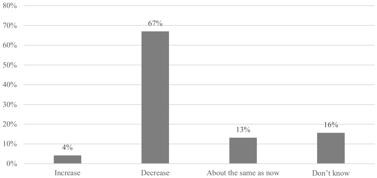
Figure 2.
Preferences regarding global production of petrochemicals. Should countries work together to decrease global production of petrochemicals such as ethylene, polyurethane, resins, and oil-based lubricants?
Figure 2.
Preferences regarding global production of petrochemicals. Should countries work together to decrease global production of petrochemicals such as ethylene, polyurethane, resins, and oil-based lubricants?
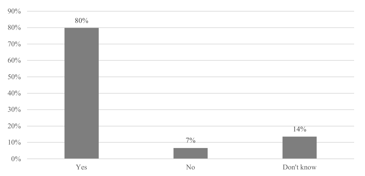
Figure 3.
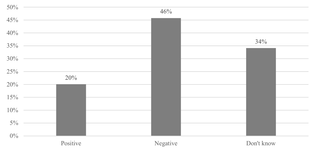
Beliefs regarding the role of petrochemicals in energy transition. On balance, what role do you think that petrochemicals (ethylene, polyurethane, resins, oil-based lubricants, etc.) can play in your country in the transition toward clean energy?
Figure 3.
Beliefs regarding the role of petrochemicals in energy transition. On balance, what role do you think that petrochemicals (ethylene, polyurethane, resins, oil-based lubricants, etc.) can play in your country in the transition toward clean energy?
The first main result is that the general public has a strongly negative view of petrochemicals: 67% believe that their country should work to decrease the demand for petrochemicals compared to only 4% supporting an increase (Figure 1), while 80% believed that the international community should work together to decrease global petrochemical production compared to only 7% calling for a collaborative increase (Figure 2).
When focusing on the clean energy transition, while a large percentage of participants professed ignorance (34%), of the majority that expressed an opinion, 46% viewed petrochemicals negatively, compared to 20% having a positive view (Figure 3).
Collectively, these results convey robust public opposition to petrochemical production, which is in stark contrast to the more ambivalent or qualified view expressed by some international experts. Accordingly, in so far as public opinion has an impact on government policy relating to petrochemicals, it is likely to be soundly negative, with participants seemingly supportive of interventions that seek to curtail the production of petrochemicals.
Future Opportunities for Petrochemicals in the Renewable Energy Transition
In all IEA energy transition scenarios, solar and wind power systems are expected to account for over 70% of global electricity capacity additions between now and 2050 (WEO [17]). In 2022, global installed wind and solar PV systems were about 2083 GW with wind turbines representing about 43.5% and solar PV accounting for 56.5%. India and China alone accounted for about 43% of the overall global installed wind turbines and solar PV. These two countries are also major sources of import demand for petrochemicals investigated in this paper. According to the IEA Net Zero Emissions Scenario (WEO [17]), global solar PV and wind turbine installed capacities are expected to cumulatively rise to about 18750 GW and 7620 GW by 2050, respectively. Future growths of installed capacities of these energy systems are anticipated to be dominated by China and India as well (WEO [17]).
If future capacity additions continue to be dominated by China and India at their current share of 43%, it is possible to evaluate potential opportunities for future petrochemical polymer material import demand in these countries if the historical import dependence is not altered significantly in the anticipated future Net Zero Transition scenario. Furthermore, considering the scale of capacity growth projected for a net-zero future, material composition data can also furnish estimates of the global petrochemical polymer requirements to manufacture these renewable energy systems. Table 10 shows the typical design attributes of solar PV and wind turbine systems, indicating the ranges of values reported by various manufacturers of these systems in their materials specification data sheets.
To quantify the petrochemical polymer demand for these energy systems, it is instructive to take a conservative approach considering the range in values of the design attributes of each system. The design attributes of focus include the unit design capacity, unit weight, and petrochemical polymer composition. Using a cautious approach, estimate of petrochemical polymer demand for the solar photovoltaic and wind turbine systems can be bounded within the range of their minimum and maximum values by applying the upper range value of their respective polymer composition to the lower range value of the unit weight of each of the energy systems. This is a reasonable approach to follow because the systems with higher compositions of petrochemical polymers are more likely to be of lighter weight, though not necessarily of lower capacity than those with lower compositions of the polymers. Light-weighting of wind turbines in particular is a known measure for energy efficiency performance improvement. Figure 3 presents the results for NZE global demand for petrochemical polymers along with the demand by China and India, and the potential import demand opportunities in both countries.
Figure 3.
Petrochemical polymer demand for energy transition under the NZE scenario.
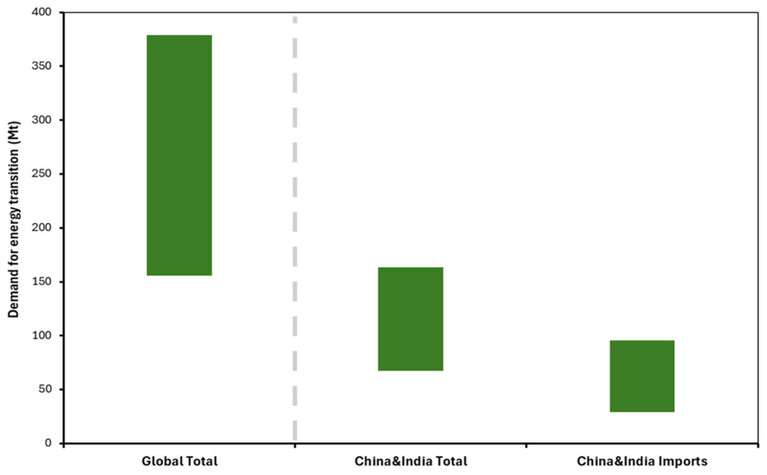
Depending on the choices of the design types of solar photovoltaic and wind turbine systems deployed globally towards achieving NZE targets by 2050, the total global petrochemical polymer demand required to manufacture those energy systems have been quantified to range between 155 to 223 million metric tons (Mt); this translates to an equivalent crude oil demand of between 0.80 to 1.13 million barrels per day over the period from 2025 to 2050), . The lower bound value represents the material requirement if only existing designs of the systems with the lowest content of petrochemical polymers are deployed in the transition, whereas the upper bound value represents the requirement if systems with the highest content of polymers are built. Similarly, China and India alone would require between 67 and 96 Mt of polymer materials for their solar and wind power systems deployments towards the global NZE ambition by 2050.
Using the estimated country-specific elasticities of import demand of petrochemical polymers with respect to annual installed solar and wind power systems capacities in China and India, the import demand of petrochemicals corresponding to the NZE transition scenario capacity additions requirements in both countries is also quantified (right of the dashed line in Figure 3). Consequently, the NZE installed capacity growth requirement of around 1150% entails additional import demand of about 67 Mt by China and India in the transition period from 2022 to 2050.
7. Concluding Remarks and Policy Insights
Many studies considered renewables and hydrocarbons as alternative sources of energy and found the negative relationship between the two. However, to date there is no dedicated applied research study estimating the impact of renewables (e.g., solar and wind) industry on demand for petrochemicals (e.g., plastics and rubber) using actual data to the best of our knowledge. In this imbalanced context, the prevailing view is that the shift towards renewable energy would diminish the demand for hydrocarbons. The survey we conducted also shows that ordinary people believe that mitigating climate change requires reducing petrochemical production.
Our study challenges this notion by empirically demonstrating that renewable energy developments could positively impact hydrocarbons, driven by the growing demand for petrochemicals. Just the capacity expansion requirements for wind and solar energy systems under IEA Net Zero scenario entails an increase in crude oil equivalent petrochemical feedstock demand of around 6%. Our primary finding, that renewables positively impact the import demand for petrochemicals, remains robust across various model specifications considered in our empirical analysis.
For policymakers in petrochemical-importing economies, the findings of this study suggest that their transition to renewables may necessitate increased demand for petrochemical imports. Furthermore, developments in domestic manufacturing and high domestic petrochemical prices could further boost this import demand. Meanwhile, policymakers in petrochemical-exporting economies should recognize the potential opportunities presented by these findings for expanding petrochemicals and related sectors. This also encompasses hydrocarbon feedstocks such as ethane, propane, butane, and naphtha that are fundamental to the petrochemical industry, and currently, there are no readily available substitutes with better environmental impact, cost-effectiveness, or efficiency for these energy transition technologies.
A parallel educational and public awareness drive may be necessary to ensure that these policies are deemed acceptable to the general public, and that ordinary people act as supportive stakeholders rather than disgruntled antagonists. The failure to do so risks forcing governments into a choice between a “productive but unpopular policy” (supporting inputs) and a “counterproductive but popular one” (curtailing inputs).
Author Contributions
FH, EU, and OA conceived the study. SM collected and processed the secondary data. FH and OA developed theoretical framing and policy interpretation. FH, EU, and OA contributed to the survey design and implementation. All authors contributed to the interpretation of the results and to writing and revising the manuscript.
Acknowledgments
We would like to thank the participants of the third ERF GCC Conference – GCC Economies in an Era of Energy Transition. Particularly. We also thank Andrea Bollino and Walid Matar for their comments and suggestions. The views expressed in this paper are those of the authors and do not necessarily represent the views of their affiliated institutions. We are responsible for any errors and omissions.
Competing Interests: The authors declare no competing interests.
Appendix A. Details of the Survey
As explained above, the survey was adapted from the UN “People’s Climate Vote” with additional questions relating to petrochemicals, specifically focusing on the demand for petrochemicals, views regarding international cooperation, and their perceived role in energy transition. Most questions were multiple choice with answers along the lines of “increase/decrease/same/don’t know”. The full questions are available in the supplement to this paper.
The survey completion platform was SurveyMonkey while the survey recruitment and distribution platform was the online system Prolific. Prolific is an online platform that connects researchers with a large, pre-screened pool of participants for academic and market research studies. Researchers design surveys or experiments and specify eligibility criteria (e.g., age, nationality, education), and Prolific recruits matching participants from its global user base. Participants are compensated for completing tasks, typically at rates aligned with ethical research standards. The platform is widely used in social science research because it provides rapid data collection, transparent sampling, and tools for screening, quality control, and demographic targeting.
In the present survey, Prolific was instructed to recruit 500 participants from each of the UK and the US, along with 1,000 participants from four countries (Brazil, Chile, India, Mexico). Three countries (China, Thailand, Turkey) from the seven studied in the empirical model were excluded because they did not have a large enough number of registrants on Prolific’s database. The UK and US were included as a benchmark. The implied sampling method is therefore non-probability, panel-based quota sampling. None of the samples were nationally representative. Participants had to complete the survey to receive compensation, meaning that there were no partially complete surveys. The survey was distributed and completed during the month of August 2025.
The original survey was in English. Participants from China and Mexico were given the option of participating in English or Spanish. Those from Brazil had the options of English and Portuguese, while those from India had the options of English and Hindi. Translation was done via machine translation with native speakers specializing in energy confirming the accuracy. Back-translation was done using a different machine learning translation platform to ensure precision.
Since the goal of the survey was to illustrate the core ideas through the data shown in Figure 1 to Figure 3, no formal statistical analysis was conducted. Given the voluntary and anonymous nature of participation (from the perspectives of the research team – Prolific knows the participants but does not transmit that information to the researchers) and the absence of tangible risks to participants, an exemption from IRB oversight was obtained (Advarra protocol Pro00083903).
References
- Elshurafa, A.; Hasanov, F.; Hunt, L. C. Macroeconomic, energy, and emission effects of Solar PV Deployment at Utility and Distributed Scales in Saudi Arabia. KAPSARC Discuss. Pap. [CrossRef]
- IEA; International Energy Agency. Assessing the effects of economic recoveries on global energy demand and CO2 emissions in 2021; Paris, 2021a. [Google Scholar]
- International Energy Agency. World Energy Outlook 2022; IEA: Paris, France, 2022; Available online: https://www.iea.org/reports/world-energy-outlook-2022.
- Genc, T.S.; Kosempel, S. Energy transition and the economy: A review article. Energies 2023, 16, 2965. [Google Scholar] [CrossRef]
- Oxford Institute for Energy Studies (OIES). Energy transition: Key challenges for incumbent players in the global energy system. 2021. Available online: https://www.oxfordenergy.org/wpcms/wp-content/uploads/2021/09/Energy-Transition-Key-challenges-for-incumbent-players-in-the-global-energy-system-ET01.pdf.
- Puyo, D.M.; Panton, A.J.; Sridhar, T.; Stuermer, M.; Ungerer, C.; Zhang, A.T. Key Challenges Faced by Fossil Fuel Exporters during the Energy Transition. Int. Monet. Fund. 2024, 001. [Google Scholar] [CrossRef]
- IPCC. Intergovernmental Panel on Climate Change. “Working Group III Contribution to the Sixth Assessment Report of the Intergovernmental Panel on Climate Change: Summary for Policymakers.”. Sixth Assessment Report, Geneva, 2022. [Google Scholar]
- Giannikopoulos, I.; Skouteris, A.; Edgar, T. F.; Baldea, M.; Allen, D. T.; Stadtherr, M. A. Probing the Impact of an Energy and Transportation Paradigm Shift on the Petrochemicals Industry. Ind. Eng. Chem. Res. 2022, 61(33), 12169–12179. [Google Scholar] [CrossRef]
- Welsby, D.; Price, J.; Pye, S.; Ekins, P. Unextractable fossil fuels in a 1.5° C world. Nature 2021, 597(7875), 230–234. [Google Scholar] [CrossRef]
- IEA; International Energy Agency. Net Zero by 2050: A Roadmap for the Global Energy Sector; Paris, 2021b. [Google Scholar]
- Kelly, H.; Hart, D. Petrochemicals Without Fossil Fuels: A National Climate-Tech Initiative. Information Technology & Innovation Foundation. 2023. Available online: https://itif.org/publications/2023/03/03/petrochemicals-without-fossil-fuels-a-national-climate-tech-initiative/.
- IEA. The Future of Petrochemicals. International Energy Agency, 2018. Available online: https://www.iea.org/reports/the-future-of-petrochemicals.
- Bennett, S.J.; Page, H.A. Implications of Climate Change for the Petrochemical Industry: Mitigation Measures and Feedstock Transitions. In Handbook of Climate Change Mitigation and Adaptation; Chen, W.Y., Suzuki, T., Lackner, M., Eds.; Springer: New York, NY. [CrossRef]
- United States Geological Survey (USGS). United States Wind Turbine Database. Wind Energy Technology Office of the Department of Energy. 2018. Available online: https://www.usgs.gov/programs/energy-resources-program/science/wind-energy.
- Rosenbloom, E. A Problem with Wind Power; Size Specifications of Common Industrial Wind Turbines. Available online: http://www.aweo.org/windmodels.html (accessed on 12 February 2024).
- Fourteau, T. Opportunities in a fossil-fuel based sector indispensable to the energy transition in Indonesia. 2022. Available online: https://www.whitecase.com/insight-our-thinking/opportunities-fossil-fuel-based-sector-indispensable-energy-transition#article-content.
- WEO. World Energy Outlook; International Energy Agency, 2023. [Google Scholar]
- WEO. World Energy Outlook; International Energy Agency, 2019. [Google Scholar]
- Guo, Z.; Sun, S.; Wang, Y.; Ni, J.; Qian, X. Impact of new energy vehicle development on china’s crude oil imports: an empirical analysis. World Electr. Veh. J. 2023, 14(2), 46. [Google Scholar] [CrossRef]
- Buchard, A.; Junkers, T. Introduction to the themed collection on sustainable polymers. Polym. Chem. 2022, 13, 1785–1786. [Google Scholar] [CrossRef]
- Adam, A.; Katsimi, M.; Moutos, T. Inequality and the import demand function. Oxf. Econ. Pap. 2012, 64(4), 675–701. [Google Scholar] [CrossRef]
- Konstantakopoulou, I. Further evidence on import demand function and income inequality. Economies 2020, 8(4), 91. [Google Scholar] [CrossRef]
- Doroodian, K. The Permanent Income Theory of Demand for Imports of Finished Manufactured Goods: The Case of the United States. Q. J. Bus. Econ. 1987, 78–85. [Google Scholar]
- Hosen, M. Z. Aggregated imports and expenditure components in Bangladesh: A cointegration and equilibrium correction analysis; Heliyon, 2023. [Google Scholar]
- Chani, M. I.; Pervaiz, Z.; Chaudhary, A. R. Determination of Import Demand in Pakistan: The Role of Expenditure Components. Theor. Appl. Econ. 2011, 18(8). [Google Scholar]
- Hendry, D. F. Deciding between alternative approaches in macroeconomics. Int. J. Forecast. 2018, 34(1), 119–135. [Google Scholar] [CrossRef]
- Castle, J.; Hendry, D. An improved approach to empirical modelling. Climate Econometrics. 2017. Available online: http://www.climateeconometrics.org/2017/02/10/an-improved-approach-to-empirical-modelling/.
- Castle, J. L.; Hendry, D. F.; Castle, J. L.; Hendry, D. F. The Polymath: Combining Theory and Data. In Modelling our Changing World; 2019; pp. 85–99. [Google Scholar]
- Hendry, D. F.; Johansen, S. Model discovery and Trygve Haavelmo’s legacy. Econom. Theory 2015, 31(1), 93–114. [Google Scholar] [CrossRef]
- Juselius, K. Searching for a theory that fits the data: A personal research odyssey. Econometrics 2021, 9(1), 5. [Google Scholar] [CrossRef]
- Juselius, K. On the role of theory and evidence in macroeconomics. In The Elgar Companion to Recent Economic Methodology; Edward Elgar Publishing, 2011. [Google Scholar]
- Campos, J.; Ericsson, N.R.; Hendry, D.F. General-to-specific modeling: An overview and selected bibliography. FRB International Finance Discussion Paper No. 838, 2005. [Google Scholar]
- Leamer, E.E.; Stern, R.M. Quantitative International Economics; Allyn and Bacon: Boston, MA, USA, 1970. [Google Scholar]
- Goldstein, M.; Khan, M.S. Income and price effects in foreign trade. In Handbook of International Economics, Volume II; Jones, R.W., Kenen, P.B., Eds.; North Holland: Amsterdam, The Netherlands, 1985; pp. 1041–1105. [Google Scholar]
- Rose, A.K.; Yellen, J.L. Is there a J-curve? J. Monet. Econ. 1989, 24, 53–68. [Google Scholar] [CrossRef]
- Rose, A.K. Exchange rates and the trade balance: Some evidence from developing countries. Econ. Lett. 1990, 34, 271–275. [Google Scholar]
- Carone, G. Modeling the US demand for imports through cointegration and error correction. J. Policy Model. 1996, 18(1), 1–48. [Google Scholar] [CrossRef]
- McKinsey (Ed.) Petrochemicals in 2022: A Return to Normalcy, with Uncertainty Ahead. McKinsey & Company, 2022. Available online: https://www.mckinsey.com/industries/chemicals/our-insights/petrochemicals-in-2022-a-return-to-normalcy-with-uncertainty-ahead.
- S; P Global. Petrochemical trends H2 2022: Petrochemical makers target resilient earnings despite market tailwinds in H2 2022. 2022. Available online: https://www.spglobal.com/commodityinsights/en/market-insights/special-reports/chemicals/petrochemical-trends-h2-2022.
- Hasanov, F.J.; Mukhtarov, S.; Suleymanov, E.; Shannak, S. The role of renewable energy and total factor productivity in reducing CO2 emissions: A case of top-ranked nations in the renewable energy country attractiveness index. J. Environ. Manag. 2024, 361, 121220. [Google Scholar] [CrossRef]
- Maddala, G.S.; Wu, S. A comparative study of unit root tests with panel data and a new simple test. Oxf. Bull. Econ. Stat. 1999, 61, 631–652. [Google Scholar] [CrossRef]
- Hadri, K. Testing for stationarity in heterogeneous panel data. Econom. J. 2000, 3, 148–161. [Google Scholar] [CrossRef]
- Pedroni, P. Critical values for cointegration tests in heterogeneous panels with multiple regressors. Oxf. Bull. Econ. Stat. 1999, 61, 653–670. [Google Scholar] [CrossRef]
- Pedroni, P. Panel cointegration: Asymptotic and finite sample properties of pooled time series tests with an application to the PPP hypothesis. Econom. Theory 2004, 20, 597–625. [Google Scholar] [CrossRef]
- Kao, C. Spurious regression and residual-based tests for cointegration in panel data. J. Econom. 1999, 90, 1–44. [Google Scholar] [CrossRef]
- Pesaran, M.H. A simple panel unit root test in the presence of cross-sectional dependence. J. Appl. Econom. 2007, 22, 265–312. [Google Scholar] [CrossRef]
- Westerlund, J. Testing for error correction in panel data. Oxf. Bull. Econ. Stat. 2007, 69, 709–748. [Google Scholar] [CrossRef]
- Hasanov, F.J.; Liddle, B.; Mikayilov, J.I. The impact of international trade on CO2 emissions in oil exporting countries: Territory vs consumption emissions accounting. Energy Econ. 2018, 74, 343–350. [Google Scholar] [CrossRef]
- Pesaran, M. H.; Smith, R. Estimating long-run relationships from dynamic heterogeneous panels. J. Econom. 1995, 68(1), 79–113. [Google Scholar] [CrossRef]
- Pesaran, M. H. Estimation and inference in large heterogeneous panels with a multifactor error structure. Econometrica 2006, 74(4), 967–1012. [Google Scholar] [CrossRef]
- Chudik, A.; Pesaran, M. H. Common correlated effects estimation of heterogeneous dynamic panel data models with weakly exogenous regressors. J. Econom. 2015, 188(2), 393–420. [Google Scholar] [CrossRef]
- Pesaran, M. H. Testing weak cross-sectional dependence in large panels. Econom. Rev. 2015, 34(6-10), 1089–1117. [Google Scholar] [CrossRef]
- Fan, J.; Liao, Y.; Yao, J. Power enhancement in high-dimensional cross-sectional tests. Econometrica 2015, 83(4), 1497–1541. [Google Scholar] [CrossRef]
- Pesaran, M. H.; Xie, Y. A bias-corrected CD test for error cross-sectional dependence in panel data models with latent factors. arXiv 2021, arXiv:2109.00408. [Google Scholar]
- Castle, J.L.; Doornik, J.A.; Hendry, D.F. Selecting a model for forecasting. Econometrics 2021, 9, 26. [Google Scholar] [CrossRef]
- Metcalf, G. E.; Stock, J. H. Measuring the macroeconomic impact of carbon taxes. In AEA papers and Proceedings; American Economic Association: Nashville, TN 37203, 2014; Vol. 110, pp. 101–106. [Google Scholar]
- Kilian, L. Not all oil price shocks are alike: Disentangling demand and supply shocks in the crude oil market. Am. Econ. Rev. 2009, 99(3), 1053–1069. [Google Scholar] [CrossRef]
- Kilian, L.; Park, C. The impact of oil price shocks on the US stock market. Int. Econ. Rev. 2009, 50(4), 1267–1287. [Google Scholar] [CrossRef]
- Gujarati, D.N.; Porter, D.C. Basic Econometrics; McGraw-Hill: New York, NY, USA, 2009. [Google Scholar]
- Bai, J.; Baltagi, B.; Pesaran, H. Cross-sectional dependence in panel data models: A special issue. 2016. [Google Scholar] [CrossRef]
- Pesaran, M. H. Time series and panel data econometrics; Oxford University Press, 2015. [Google Scholar]
- Baltagi, B.H.; Pesaran, M.H. Heterogeneity and cross section dependence in panel data models: Theory and applications introduction. J. Appl. Econom. 2007, 22, 229–232. [Google Scholar] [CrossRef]
- Korniejenko, K.; Kozub, B.; Bąk, A.; Balamurugan, P.; Uthayakumar, M.; Furtos, G. Tackling the circular economy challenges—Composites recycling: Used tyres, wind turbine blades, and solar panels. J. Compos. Sci. 2021, 5, 243. [Google Scholar] [CrossRef]
- International Energy Agency. The Oil and Gas Industry in Net Zero Transitions; IEA: Paris, France, 2023; Available online: https://www.iea.org/reports/the-oil-and-gas-industry-in-net-zero-transitions.
- Halawani, Z. A.; Al Dabbagh, M. A. Petrochemical polymers and technical textile industry in the Kingdom of Saudi Arabia. Fibres Text. 2020, 27(2), 96–102. [Google Scholar]
- Raj, T.; Chandrasekhar, K.; Kumar, A. N.; Kim, S. H. Recent biotechnological trends in lactic acid bacterial fermentation for food processing industries. Syst. Microbiol. Biomanufacturing 2021, 1–27. [Google Scholar] [CrossRef]
- Mangaraj, S.; Yadav, A.; Bal, L. M.; Dash, S. K.; Mahanti, N. K. Application of biodegradable polymers in food packaging industry: A comprehensive review. J. Packag. Technol. Res. 2019, 3, 77–96. [Google Scholar] [CrossRef]
- Latunussa, C.; Mancini, L.; Blengini, G.; Ardente, F.; Pennington, D. Analysis of material recovery from silicon photovoltaic panels. EUR 27797; Publications Office of the European Union: Luxembourg (Luxembourg), 2016; p. JRC100783. Available online: https://publications.jrc.ec.europa.eu/repository/handle/JRC100783.
- Dominish, E.; Florin, N.; Teske, S. Responsible Minerals Sourcing for Renewable Energy. Report prepared for Earthworks by the Institute for Sustainable Futures, University of Technology Sydney. 2019. Available online: https://earthworks.org/assets/uploads/2019/04/MCEC_UTS_Report_lowres-1.pdf.

Table 1.
Variables used in the study.
| Variable | Definition | Measurement | Source |
| Imports of Petrochemicals (MP) | The import volumes of the petrochemical products of rubber and plastic. | Thousand tons | United Nation Commodity Trade database (UNCOMTRADE). |
| Renewable Energy Installed Capacity (REIC) | The installed capacity of solar and wind power systems. | Megawatts | Statistical Review of World Energy, 2023 release. |
| Income (Y) | Manufacturing value added. | Million US$ at 2015 constant prices | WDI database, 2023 release. |
| Relative Prices (PR) | The ratio of the international prices of rubber and plastic to domestic prices. The international price of rubber and plastic is calculated as the ratio of value of these products in thousand US$ to their volume in thousands of tons. The resulting series is divided by the figure in 2015 to get index as 2015=100. The domestic price is represented by the GDP deflator, 2015=100. This is dictated by the data availability, as we could not find either domestic petrochemical prices or manufacturing/industry prices for all countries and sample span under consideration. | Index, 2015=100 | The value and volume of rubber and plastic are from UNCOMTRADE. GDP deflator data are from WDI database, 2023 release. |
Table 2.
Descriptive statistics of the variables.
| Country | MP, in thousand tons | REIC, in Megawatts | ||||
| Mean | Max | Min | Mean | Max | Min | |
| Brazil | 1595.20 | 2236.89 | 790.77 | 7072.24 | 48241.99 | 0.00 |
| Chile | 140.22 | 197.87 | 44.70 | 1473.25 | 10080.12 | 0.00 |
| China | 18009.07 | 36100.30 | 2945.83 | 141037.83 | 759092.13 | 1.00 |
| India | 2377.18 | 4635.83 | 550.62 | 25058.14 | 105075.86 | 0.00 |
| Mexico | 2340.98 | 5306.39 | 949.67 | 3215.56 | 16338.55 | 10.00 |
| Thailand | 9157.34 | 14264.14 | 4717.03 | 1243.68 | 4610.60 | 0.00 |
| Turkey | 1510.27 | 3565.57 | 223.93 | 4258.76 | 20822.62 | 0.00 |
| Panel | 5018.61 | 36100.30 | 44.70 | 26194.21 | 759092.130 | 0.00 |
| Notes: Max and Min denote maximum and minimum values; there are 27 annual times series observations from 1996 to 2022 for each variable in each country. | ||||||
Table 3.
Methods to be considered.
| Method | PURT | PCT | Long-run Estimation | Short-run Estimation |
| First Generation | Maddala and Wu [41] Hadri [42] |
Pedroni [43,44], Kao [45] |
PDOLS, PFMOLS, MG or PMG |
PECM or PDR with GTSMS |
| Second Generation | Pesaran [46] | Westerlund [47] | CCEMG or CCEP AMG |
|
| Note. PURT=Panel Unit Root Test; PCT=Panel Cointegration Test; PDOLS=Panel Dynamic Ordinary Least Squares, PFMOLS=Panel Fully Modified Ordinary Least Squares, MG=Mean Group; PMG=Polled Mean Group, CCEMG=Common Correlation Effect Mean Group; CCEP= Common Correlation Effect Pooled; PECM=Panel Error Correction Model; PDR=Panel Dynamic Regression; GTSMS=General to Specific Modeling Strategy. | ||||
Source: Re-produced from Hasanov et al. [48].
Table 4.
The results of the CD tests.
| Variables | Pesaran [52] | Fan et al. [53] | Pesaran and Xie [54] |
| mp | 27.93*** | 185.84*** | -1.73* |
| reic | 32.18*** | 213.83*** | -3.60*** |
| y | 20.22*** | 100.80*** | 1.64* |
| pr | 20.24*** | 144.66*** | 0.54 |
| Notes: *, **, and *** indicate rejection of the null hypothesis of weak CD in favour of the alternative hypothesis of strong CD at the 1%, 5%, and 10% significance levels, respectively. | |||
Table 5.
The results of the Pesaran [46] panel unit root test.
Table 5.
The results of the Pesaran [46] panel unit root test.
| Variables | Level | First difference | Second difference |
| CIPS | CIPS | ||
| mp | 0.239 (0.594) | -6.033 (0.000) *** | |
| reic | -0.378 (0.353) | -3.573 (0.000) *** | |
| es | 0.495 (0.690) | -3.443 (0.000) *** | |
| y | -0.293 (0.385) | -3.839 (0.000) *** | |
| pr | -0.967 (0.167) | -0.551 (0.291) | -7.597 (0.000) *** |
| Notes: *, **, and *** indicate rejection of the null hypothesis of unit root in favour of the alternative hypothesis of (trend) stationarity at the 1%, 5%, and 10% significance levels, respectively. The values in the table are the Z statistics from the cross-sectionally augmented Im-Pesaran-Shin (CIPS) test by Pesaran [46] and values in the parentheses are the associated probabilities. The CIPS test assumes cross-section dependence in the form of a single unobserved common factor. The test equation includes intercept and time trend in testing the level of the variables while they include intercept only for the testing the first (or second) difference of the levels. This is based on the statistical significance of the mentioned deterministic regressors. The lag order of one is selected to remove serial correlation from the residuals of the test equation. | |||
Table 6.
The results of the Westerlund [47] panel cointegration test.
Table 6.
The results of the Westerlund [47] panel cointegration test.
| Statistics | Gt | Ga | Pt | Pa |
| Sample value | -1.794 | -8.989** | -7.189** | -12.393*** |
| p-values | 0.300 | 0.025 | 0.013 | 0.000 |
| Notes: *, **, and *** indicate rejection of the null hypothesis of no cointegration in favour of the alternative hypothesis of cointegration at the 1%, 5%, and 10% significance levels, respectively. Westerlund [47] cointegration tests were performed without intercept and trend, as this was dictated by the statistical significance of the deterministic components in the test equations. To address the CD effect and get robust probability values, the test is run with bootstrap (80 values). | ||||
Table 7.
The polled long-run estimation results for the panel of 7 countries.
| Regressor | Constant | d_prit | yit | reicit |
| 14.519* (0.125) |
-1.028** (0.068) |
0.660 (0.430) |
0.195*** (0.037) |
|
| Notes: Dependent variables is mpit. *, **, ***, and **** indicate rejection of the null hypothesis of no statistical significance at the 16%, 10%, 5% and 1% significance levels, respectively. Numbers in the parentheses are the associated probabilities. Exclusion of the time trend in the estimations was because of its statistical insignificance. Number of observations = 27 (Time series observations) x 7 (Number of countries) = 189. | ||||
Table 8.
Country-specific long-run elasticities of installed renewable capacity.
| Country | reict | P-value |
| Brazil | 0.178**** | (0.000) |
| Chile | 0.047 | (0.724) |
| China | 0.610** | (0.064) |
| India | 0.452 | (0.224) |
| Mexico | 0.086* | (0.134) |
| Thailand | 0.021 | (0.377) |
| Turkey | 0.211*** | (0.030) |
| Slope Heterogeneity Test: | ||
| Adjusted test value: 4.773**** (0.000) | ||
| Notes: Dependent variable is mpt. P-values are in parentheses. *, **, ***, and **** indicate rejection of the null hypothesis of no statistical significance at the 16%, 10%, 5% and 1% significance levels, respectively. T=27. Exclusion of the time trend from the estimations was because of its statistical insignificance. We did not exclude constant if it is statistically insignificant because it is hard to assume that MP initial level is zero. | ||
Table 9.
The long-run estimation results from reduced forms of equation (2.3).
| Regressor | Cit | d_prit | yit | reicit |
| Model 1 | 2.662**** (0.004) |
-0.500 (0.678) |
--- | 0.173**** (0.008) |
| Model 2 | 20.122*** (0.004) |
--- | 0.697 (0.263) |
0.165*** (0.046) |
| Model 3 | 2.611**** (0.004) |
--- | --- | 0.200*** (0.024) |
| Model 4 | -5.470 (0.591) |
-0.167 (0.913) |
0.508 (0.425) |
--- |
| Notes: Dependent variables is mpit. Cit is the country specific intercept *, **, *** and **** indicate rejection of the null hypothesis of no statistical significance at the 16%, 10%, 5% and 1% significance levels, respectively. | ||||
| Equation (2.3): Model 1: Equation (2.3) without yit; Model 2: Equation (2.3) without d_prit; Model 3: Equation (2.3) without yit and d_prit; Model 4: Equation (2.3) without reicit; | ||||
| Exclusion of the time trend in the estimations was based on its statistical significance. We did not exclude constant if it is statistically insignificant because it is hard to assume that MP initial level is zero. Number of observations = 27 (Time series observations) x 7 (Number of countries) = 189. | ||||
Table 10.
Design attributes of typical solar PV and wind turbine systems.
| Attribute | Renewable Energy System | Sources | |
| Solar Photovoltaic | Wind Turbine | ||
| Unit design capacity | 0.25 – 0.5 kilowatts | 1.5 – 5.0 megawatts | Latunussa et al. [68], Dominish et al. [69], USGS [14], Rosenbloom [15]. |
| Unit weight | 18.14 – 34.93 kilograms | 150 – 485 metric tons | |
| Polymer composition | 6.6 – 10% | 11 – 16% | |
Disclaimer/Publisher’s Note: The statements, opinions and data contained in all publications are solely those of the individual author(s) and contributor(s) and not of MDPI and/or the editor(s). MDPI and/or the editor(s) disclaim responsibility for any injury to people or property resulting from any ideas, methods, instructions or products referred to in the content. |
© 2026 by the authors. Licensee MDPI, Basel, Switzerland. This article is an open access article distributed under the terms and conditions of the Creative Commons Attribution (CC BY) license.
Copyright: This open access article is published under a Creative Commons CC BY 4.0 license, which permit the free download, distribution, and reuse, provided that the author and preprint are cited in any reuse.