Live Imaging Approach for Quantitative Characterization of Transcription Factor Properties

Introduction

Materials

• Fly line having the protein of interest tagged with a fluorescent protein and histone tagged with a spectrally distinct fluorescent protein
• For tagged His2Av, existing stocks such as w[*]; P{w[+mC]=His2Av-mRFP1}II.2 (BDCS# 23651) for RFP tagged His2Av or w[*]; P{w[+mC]=His2Av-EGFP.C}2/SM6a (BDSC# 24163) for GFP tagged His2Av can be used. Lines with His2Av tagged with BFP are also available in the fly community [19].

• Vials with molasses media (Archon Scientific, Catalog # B20101)
• Embryo Collection Cages (Flystuff® Drosophila Embryo Collection Cages, Genesee Scientific Catalog # 59-105)
• Petri dish (VWR Catalog # 10799-192)
• Grape juice agar
• Active dry yeast (VWR Catalog # 470303-062)
• Incubator that can be set to 25 °C
• Deionized water

• Mesh basket with 1” inside diameter (Flystuff® Drosophila Mesh Baskets, Genesee Scientific Catalog # 46-102)
• Mesh with pore size 120 µm (Flystuff® Drosophila Mesh, Genesee Scientific Catalog # 57-102)
• Paint brush (size 1-2)
• Deionized water
• Bleach (Clorox® Concentrated Germicidal Bleach, VWR Catalog # 89501-620)

• Paint brush (size 1-2)
• Stereo microscope
• Hair loop (prepared by looping a human hair and attaching it to a pipette tip with a piece of tape)
• Glass bottom dish, 35 mm Dish, No. 1.5 Coverslip, 20 mm Glass Diameter, Uncoated (Mattek, VWR Catalog # MSPP-P35G1520C)
• Deionized water
• Low melting point agarose (IBI Scientific, VWR Catalog # IB70050)
• Clear double-sided tape (Scotch, VWR Catalog # 500026-846)
• Heptane (VWR Catalog # MK513910)
• Microscope slides 75×25×1 mm (VWR Catalog # 16004-422)
• Cover glass 50×24×0.2 mm
• TetraSpeck beads (0.1 µm, T7279, Invitrogen)
• Ethanol (VWR Catalog # EM-EX0276-4S)

• Confocal microscope (LSM 900, Carl Zeiss, Germany) with

  ○

  40x objective (C-Apochromat 40x/1.2 water immersion Korr objective)

  ○

  Lasers depending on the fluorescent proteins (488 nm laser for GFP and 561 nm laser for RFP)

• ZEN Microscopy Software

• Fiji (ImageJ)
• MATLAB R2024a (MathWorks)

Methods

• Flies are harvested on a standard cornmeal-molasses-yeast diet at a 25 °C incubator in room with 12 h light/dark cycle
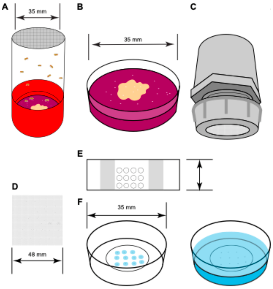
• Embryo collection cages are set with flies required to produce embryos containing desired proteins of interest tagged with fluorescent proteins two days before imaging (Figure 1A)
• Yeast paste is prepared by adding and mixing deionized water with active dry yeast
• The grape juice agar plates are streaked with yeast paste (grape juice plate streaked with yeast paste are referred to as plates henceforth)
• The plate is placed on the bottom of the cage for oviposition
• The plates are changed twice every day for two days before imaging is started
• To remove any older eggs which are often retained by the females before deposition, a plate is placed in the cage for an hour of pre-egg laying session
• After one hour the plate is replaced with another plate to collect embryos for two hours.
• After the embryo collection, the plate is removed and replaced with another plate
• The deposited embryos should be appropriately aged by placing the plate in an incubator at 25 °C so the desired stage for the experiments is reached. For nuclear cycle 14, the embryos should be aged at 25 °C for two hours (Figure 1B).

• Mesh is placed inside mesh baskets for embryo collection
• After aging, the embryos are transferred to the mesh basket and rinsed with deionized water from a wash bottle that filters out any residual yeast paste (Figure 1C)
• A Petri dish is filled three-quarters full with fresh bleach
• The embryos contained in the mesh basket is submerged in the bleach for 30 seconds for dechorionation
• After 30 seconds, the embryos in the mesh basket are rinsed with about 250 ml deionized water from a wash bottle to make sure all the residual bleach is removed
• The mesh containing the washed and dechorionated embryos is removed from the basket (Figure 1D)

• Appropriate immersion medium is used on the objective. In this case, a drop of water is pipetted on the 40x/1.2 objective
• The sample in the slide or glass bottom dish is placed on the microscope stage
• The focus is adjusted to view the surface of an embryo at appropriate stage
• Imaging parameters are selected

  ○

  Image is acquired by raster scanning where the laser moves unidirectionally, forming the image by linear scanning followed by line retracing

  ○

  Frame size 1024 pixels by 1024 pixels

  ○

  Pixel size of 31.95 nm obtained at 5x zoom

  ○

  Pixel dwell time of 2.06 µs, which results in a frame time of 5.06 s

  ○

  0.2% laser power are selected for both 488 nm laser and 561 nm laser. Laser power should be selected based on the intensity observed in both the channels for the proteins of interest and should be balanced to improve the signal-to-noise ratio but minimize photobleaching.

• The focus is adjusted to view the nuclei on the surface of the embryo.
• Time series acquisition is started after selecting the microscope parameters.
• Time series acquisition of at least 12 frames is taken per region of interest (ROI)
• If a longer time course is needed, the ROI can be moved to a different part of the embryo expected to have similar behavior as those in the current ROI
• Owing to the higher surface area of the embryo along anteroposterior (AP) direction compared to that in the dorsoventral (DV) direction, it is possible to move the ROI to a location along the AP direction after each acquisition.

  ○

  For ubiquitously expressed proteins, this enables long time course to be obtained with minimal photobleaching

  ○

  If the protein shows DV variation but no AP variation, a similar long time course is enabled by moving along the AP direction. And for observing the spatial variation along DV, embryos mounted at different DV coordinate need to be imaged

  ○

  If the protein shows AP variation but no DV variation, by changing the location of the ROI, the spatial variation along AP is obtained. If a long time course is needed at a particular AP position, photobleaching correction should be considered if a high laser power is used.

• 70% ethanol is added to diffraction-limited TetraSpeck beads for a 1:1000 dilution.
• The beads are uniformly suspended by sonicating in water bath for 20 minutes.
• The suspension is mounted following the same procedure as embryos:

  ○

  Using glass bottom dish: 5 µl of the suspension is added to the glass bottom dish and it is allowed to dry. 1% low melting point agarose solution is added over the dried sample and allowed to solidify. Then a thin layer of water is added over the agarose.

  ○

  Using slide with coverslip: 5 µl of the suspension is add to a slide and it is allowed to dry. 5 µl of water is added over the dried sample and covered with a coverslip.

• Same objective and microscope settings are used to obtain the images as mentioned in the point 4 of Image acquisition.
• An ROI is selected in which the beads are sparsely distributed far apart one another.
• z-stack is acquired with the imaging volume extending beyond the beads on both sides to include regions with minimal fluorescence signal. Each slice is separated by 0.05 microns, yielding around 80 slices in total.
• Three acquisitions are taken per batch of the mounted beads by repositioning the ROI to previously unimaged areas.
• The acquisition is repeated for three batches of mounted beads.
• For the PSF analysis, open the “run_fitPSF3D.m” file. The script calls the function “fitPSF3D.m” which loads the images in the specified file path, detects the fluorescent beads in the specified channel, fits a 3D Gaussian function to each bead, and saves the fitted parameters in the specified output folder path.

  ○

  The beads are detected in the average z projection image. The center of each bead (x and y coordinates) and the z-slice with the maximum intensity for each bead are used as an initial guess for the Gaussian fitting using lsqcurvefit. The fitted parameters include the bead center coordinates along each axis, standard deviations along each axis, amplitude, and background intensity. These parameters for each .czi file are saved in separate .mat files in the output folder. An average z-projection image for each CZI file is also saved as a .tif file.

• Open the “sc_main.m” file. This script will run the code to load the images, segment nuclei from the images, calculate the ACFs and CCFs, and fit a series of biophysical models to the ACFs and CCFs.
• The top of “sc_main.m” contains a series of editable options, including the image path and filename, size of the point spread function (PSF), background subtraction and image stabilization flags, the sliding window size for image grouping and averaging, and the channel numbers for the data and mask channels. A guess of the diffusivity of mobile components can also be chosen. The default values for everything except the image path and filename are pre-filled.
• The first block of code loads the image series. If the background subtraction and stabilization flags are set to “true,” these processes will also occur in this block of code. If the image series is tiled, the frames from each tile will be grouped into separate elements of a cell variable in Matlab.
• In the second block of code, the nuclei are segmented in the image. To increase robustness, groups of 7-12 frames are averaged together and the segmentation is performed on the averaged image. The nuclear segmentation mask is eroded by 0.5 microns to provide a conservative estimate of the nuclei, decreasing the probability of false positives. Similarly, the complement of the pre-eroded mask is the cytoplasmic mask, which is then also eroded by 0.5 microns to provide a conservative estimate of the cytoplasm.
• In the next block of code, the ACFs and CCF are calculated for each time point. The time points may consist of different tiles in the image or of groups of 7-12 image frames. ACFs are calculated for the total, nuclear, and cytoplasmic fractions of the data channel, and for the nuclear fraction of the nuclear channel. The CCF between the data and nuclear channel is calculated for the nuclear fraction.
• The next block of code fits the ACFs, or portions of the ACFs, to three models, resulting in estimated parameters:

  ○

  First, the fast direction of each ACF is fit to a Gaussian-shaped model of the PSF. This allows us to infer the amplitude of each ACF, which in turn allows us to infer absolute concentrations of the fluorescent species.

  ○

  Second, each full ACF is fit to a pure diffusion model, allowing us to estimate an effective overall diffusivity. This model is typically inaccurate as most species contain a mixture of mobile and immobile components.

  ○

  Third, each full ACF is fit to a two-component model, which accounts for a potential mixture of a single mobile component and one immobile component. This model estimates the fraction of the immobile component and the diffusivity of the mobile component. This fit may not accurately identify the diffusivity, as in some cases, it is unidentifiable. It is recommended to set a moderate value of the diffusivity, such as 3-5 μm²/s.

• The next block of code fits the CCF to a model specific to the CCF. As the CCF includes cross-correlation between a TF and histone, and likely represents TF bound to DNA, this model assumes a near-zero diffusivity. This model includes corrections for differences in volume and centroid location of the PSFs of the two imaged wavelengths. This model allows us to estimate the fraction of the TF that is bound to DNA.
• The final block of code produces a plot of the results

  ○

  For single time point acquisitions, the resulting plots include the ACFs and the CCF, and annotates the plots with the estimated model parameters (absolute concentration, diffusivity, immobile fraction, DNA-bound fraction).

  ○

  For time course acquisitions, the resulting plots include the estimated model parameters as functions of time.

• The final output data, including nuclear segmentation masks, ACFs, CCFs, image metadata (czi path and filename, image size, time step, pixel dwell time, etc.) and the chosen analysis flags (background subtraction, stabilization, etc), are stored as a structure variable. A separate structure variable, which also stores the image metadata and chosen flags, is produced that contains the estimated parameters. These two structures are kept separate due to the large size of the ACFs and CCFs stored in the first structure variable.
• If multiple image series are analyzed, the above structure variables for each image series should concatenated for visualization purposes (see below).
• Visualization of results
• To produce a plot of averages of the estimated parameters from either multiple time course acquisitions, or multiple acquisitions at different spatial locations, run “sc_extract_RICS_timecourse.m” or “sc_extract_RICS_spatialorientation.m”, respectively.
• For visualization of time courses, run “sc_extract_RICS_timecourse.m”. This script will first load the concatenated structure variable containing the time courses of estimated parameters (including absolute concentration, diffusivity, immobile fraction, DNA-bound fraction of the TF). In the beginning of the script, you must specify the path to a mat file containing this structure variable. The script then calls “extract_RICS_timecourse”, which outputs a structure variable that contains the time course of estimated parameters, averaged across all embryos. Error bars are also calculated. You can set a flag to have the error bars represent standard deviation or standard error of the mean. You can also set a flag to have the script plot the averaged time courses.
• For visualization of spatial variation, run “sc_extract_RICS_timecourse.m”. This script largely parallels the script discussed in the previous point. It will first load the concatenated structure variable containing the estimated parameters (including absolute concentration, diffusivity, immobile fraction, DNA-bound fraction of the TF) for each RICS acquisition. In the beginning of the script, you must specify the path to a mat file containing this structure variable. You must also supply the spatial location for each acquisition. The script outputs a structure variable that contains the estimated parameters, binned into different spatial locations. Error bars for each bin are also calculated. As with the previous script, you can set a flag to have the error bars represent standard deviation or standard error of the mean. You can also set a flag to have the script plot the binned values of the parameters.

References

1. Li, X.-Y.; Thomas, S.; Sabo, P. J.; Eisen, M. B.; Stamatoyannopoulos, J. A.; Biggin, M. D. The role of chromatin accessibility in directing the widespread, overlapping patterns of Drosophila transcription factor binding. Genome Biol. 2011, 12, R34. [Google Scholar] [CrossRef]
2. Spitz, F.; Furlong, E. E. M. Transcription factors: from enhancer binding to developmental control. Nat. Rev. Genet. 2012, 13, 613–626. [Google Scholar] [CrossRef]
3. Mir, M.; Reimer, A.; Haines, J. E.; Li, X.-Y.; Stadler, M.; Garcia, H.; Eisen, M. B.; Darzacq, X. Dense Bicoid hubs accentuate binding along the morphogen gradient. Genes Dev. 2017, 31, 1784–1794. [Google Scholar] [CrossRef]
4. Mir, M.; Stadler, M. R.; Ortiz, S. A.; Hannon, C. E.; Harrison, M. M.; Darzacq, X.; Eisen, M. B. Dynamic multifactor hubs interact transiently with sites of active transcription in Drosophila embryos. Elife 2018, 7, e40497–e40497. [Google Scholar] [CrossRef]
5. Dima, S. S.; Turner, M. A.; Garcia, H. G.; Reeves, G. T. Global maps of transcription factor properties reveal threshold-based formation of DNA-bound and mobile clusters. Sci. Adv. 2026, 12, eady3909. [Google Scholar] [CrossRef]
6. Munshi, R.; Ling, J.; Ryabichko, S.; Wieschaus, E. F.; Gregor, T. Transcription factor clusters as information transfer agents. Sci. Adv. 2025, 11, eadp3251. [Google Scholar] [CrossRef]
7. Zhang, L.; Hodgins, L.; Sakib, S.; Verbeem, A.; Mahmood, A.; Perez-Romero, C.; Marmion, R. A.; Dostatni, N.; Fradin, C. Both the transcriptional activator, Bcd, and repressor, Cic, form small mobile oligomeric clusters. Biophys. J. 2024. [Google Scholar] [CrossRef]
8. Digman, M. A.; Brown, C. M.; Sengupta, P.; Wiseman, P. W.; Horwitz, A. R.; Gratton, E. Measuring fast dynamics in solutions and cells with a laser scanning microscope. Biophys. J. 2005, 89, 1317–1327. [Google Scholar] [CrossRef]
9. Digman, M. A.; Sengupta, P.; Wiseman, P. W.; Brown, C. M.; Horwitz, A. R.; Gratton, E. Fluctuation correlation spectroscopy with a laser-scanning microscope: Exploiting the hidden time structure. Biophys. J. 2005, 88, L33–L36. [Google Scholar] [CrossRef]
10. Digman, M. A.; Gratton, E. Analysis of diffusion and binding in cells using the RICS approach. Microsc. Res. Tech. 2009, 72, 323–332. [Google Scholar] [CrossRef]
11. Schloop, E.; Hiremath, S. V.; Shaikh, R.; Williams, C. M.; Reeves, G. T. Spatiotemporal dynamics of NF-κB/Dorsal inhibitor IκBα/Cactus in Drosophila blastoderm embryos. bioRxiv 2024. [Google Scholar] [CrossRef]
12. Brown, M.; Dalal, R. B.; Hebert, B.; Digman, M. A.; Horwitz, A. R.; Gratton, E. Raster image correlation spectroscopy (RICS) for measuring fast protein dynamics and concentrations with a commercial laser scanning confocal microscope. J. Microsc. 2008, 229, 78–91. [Google Scholar] [CrossRef]
13. Al Asafen, H.; Clark, N. M.; Goyal, E.; Jacobsen, T.; Dima, S. S.; Chen, H.-Y.; Sozzani, R.; Reeves, G. T. Dorsal/NF-κB exhibits a dorsal-to-ventral mobility gradient in the Drosophila embryo. eLife 2024, 13, RP100462. [Google Scholar] [CrossRef]
14. Magde, D.; Webb, W. W.; Elson, E. L. Fluorescence correlation spectroscopy. III. Uniform translation and laminar flow. Biopolymers 1978, 17, 361–376. [Google Scholar] [CrossRef]
15. Dima, S. S.; Reeves, G. T. Bulk-level maps of pioneer factor binding dynamics during the Drosophila maternal-to-zygotic transition. Development 2025, 152, dev204460. [Google Scholar] [CrossRef]
16. Dima, S. S.; Reeves, G. T. Genome-wide mapping of Bicoid/DNA interactions reveals quantitative constraints on transcriptional regulation. In Developmental Biology [Preprint]; 2026. [Google Scholar] [CrossRef]
17. Bacia, K.; Schwille, P. Practical guidelines for dual-color fluorescence cross-correlation spectroscopy. Nat. Protoc. 2007, 2, 2842–2856. [Google Scholar] [CrossRef]
18. Weidemann, T.; Wachsmuth, M.; Tewes, M.; Rippe, K.; Langowski, J. Analysis of ligand binding by two-colour fluorescence cross-correlation spectroscopy. Single Mol. 2002, 3, 49–61. [Google Scholar] [CrossRef]
19. Lim, B.; Heist, T.; Levine, M.; Fukaya, T. Visualization of Transvection in Living Drosophila Embryos. Mol. Cell 2018, 70, 287–296.e6. [Google Scholar] [CrossRef]
20. Turner, M. A.; Gravina, N. M.; Moretti, B.; Dima, S.; Martini, G.; Reeves, G.; Garcia, H. G. Novel Fluorescent and Photoconvertible Fusions Reveal Dorsal Activator Dynamics. Dev. Biol. [Preprint] 2025. [Google Scholar] [CrossRef]
21. Nyberg, K. G.; Carthew, R. W. “CRISPR-/Cas9-Mediated Precise and Efficient Genome Editing in Drosophila” in Methods in Molecular Biology; Humana Press Inc., 2022; vol. 2540, pp. 135–156. [Google Scholar]
22. Supatto, W.; McMahon, A.; Fraser, S. E.; Stathopoulos, A. Quantitative imaging of collective cell migration during Drosophila gastrulation: multiphoton microscopy and computational analysis. Nat. Protoc. 2009, 4, 1397–1412. [Google Scholar] [CrossRef]