

Submitted:
02 November 2026
Posted:
05 November 2026
You are already at the latest version
Abstract
Network science frequently seeks general laws of connectivity that persist across scales and disciplines, regardless of specific edge weights. A primitive in this setting is the computation of unweighted all-pairs shortest paths (APSP), which underlies measures of distance, centrality [1], and navigability [2]. However, the canonical Zuse-Moore breadth-first search (ZM-BFS) [3,4] algorithm is prohibitively slow for large and dense networks. Here, leveraging network science principles [2], we introduce CC-BFS: a dynamic programming algorithm for APSP. By prioritizing influential hubs, memoizing intermediate results and exploiting network hierarchy, CC-BFS drastically reduces computational effort, with up to 2500× speedup over ZM-BFS on scale-free networks. Furthermore, CC-BFS substantially outperforms the state-of-the-art direction-optimizing BFS (DO-BFS) [5] across diverse artificial and real-world benchmarks, while utilizing around 80% less memory. In practice, solving the APSP problem on dense and scale-free topologies can approach a time complexity of 0 (n2.5) and in networks with 100,000 nodes passes from over 2 days for ZM-BFS to around 2 minutes for CC-BFS, which represents a milestone potentially impacting many domains of science. CC-BFS scales across shared-memory threads and generalizes to related problems like computing network diameter and radius. By integrating network science into algorithm design, CC-BFS overcomes long-standing scalability challenges, opening new avenues for network-based computational analysis.
Keywords:
all-pairs shortest path
; network science
; dynamic programming
; breadth-first search
; scale-free networks
Introduction
Network science offers a formalism for understanding how structure, dynamics and function co-emerge in complex systems, ranging from socio-economic [6] and biological networks [7,8] to artificial intelligence (AI) [9,10]. Yet, the slowing pace of Moore’s law [11], coupled with the explosive growth of network-structured data, demands efficient algorithms for large-scale complex networks.
From social networks to brain connectomes and molecular interactomes, one of the enduring goals of network science is to identify shared principles of connectivity that generalize across systems and scales [12,13,14,15]. For many questions, this entails moving beyond system-specific link weights or directions to characterize connectivity principles that rely solely on the information encoded by network topology [12,13,14,15]. Hence, from here forward, unless otherwise specified, we will intend all networks and operations defined on them as unweighted and undirected. A core primitive in this setting is the computation of all-pairs shortest paths (APSP), which underlies measures of distance, centrality [1], and navigability [2]. For instance, an important application of the APSP problem is the estimation of characteristic path length (i.e., the mean unweighted shortest-path length), a key metric for modelling [12] and characterizing [16] the small-world phenomenon in complex systems—ranging from social networks [17] to brain connectomes [18].
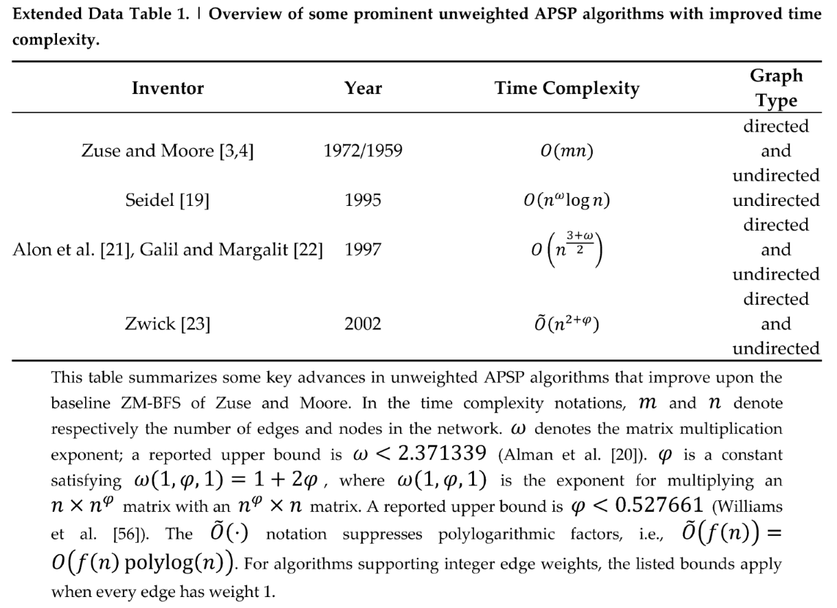
The widely employed Zuse-Moore algorithm [3,4] (ZM-BFS) solves APSP by executing n single-source breadth-first searches (BFS) in O(mn) time (m edges, n nodes). The state-of-the-art direction-optimizing BFS (DO-BFS) [5] accelerates each search by switching, level by level, between conventional top-down expansion from the frontier and a bottom-up step in which unvisited nodes look for a parent in the frontier. This avoids many redundant edge examinations in low-diameter networks, but each search still runs independently, so DO-BFS does not improve on the O(mn) bound. Substantial theoretical progress has also been made beyond this O(mn) bound (Extended Data Table 1). Using fast matrix multiplication (FMM), Seidel’s algorithm [19] achieves O(nωlogn) time, where ω denotes the matrix multiplication exponent, with the bound ω < 2.371339 [20]. Alon et al. [21] and Galil and Margalit [22] obtained time, and Zwick [23] improved this bound to using bridging sets and rectangular matrix multiplication. Here, suppresses polylogarithmic factors, and φ is determined by the rectangular multiplication exponent (Extended Data Table 1). Among the prominent bounds listed, Seidel’s is the strongest for dense networks where m~n2. However, these theoretical bounds generally do not translate into practical speedups because the FMM routines required to attain them carry very large constant factors. For example, FMM routines approaching ω ≈ 2.37 are widely regarded as “galactic” [24], with practical speedups expected only at impractically large matrix sizes [25]. Moreover, they are poorly suited to the sparse networks ubiquitous in real systems, where m~n and ZM-BFS already runs in O(n2) time. This gap between theory and practice underscores the need for algorithms that are both asymptotically efficient and practically scalable.
Here, we demonstrate that this gap can be bridged by leveraging network science principles of decomposition, prioritization, and memoization, previously explored by Cannistraci et al. [2] Building on these principles, we introduce Cannistraci-Chen BFS (CC-BFS), a dynamic programming variant of BFS. It operates through the three synergistic principles: decomposition breaks down APSP into heterogeneous single-source search (SSS) subproblems around a few influential hub nodes; prioritization orders these subproblems to maximize computational benefit from information reuse; and memoization captures and propagates SP information across subsequent searches, exploiting the dependencies created by decomposition and prioritization.
Specifically, the algorithm employs four optimization techniques: First, vector comparison (VC)-based memoization captures and reuses SP distance information from earlier computations, avoiding redundant exploration in subsequent searches. Second, hub-guided memoization selectively constructs SP structures for a few influential hub nodes, enabling efficient propagation of SP information to their neighboring sources. Third, a direction-adaptive propagation strategy dynamically switches between forward and backward search directions based on estimated edge-examination costs. Finally, topology-based distance data typing mitigates the memory bottleneck: by first bounding the network diameter, CC-BFS allocates the smallest sufficient data type for the distance matrix and cuts the memory footprint often by 4× to 8× versus double-precision storage.
This integration yields substantial performance gains while maintaining conceptual simplicity and scalability. On scale-free networks, CC-BFS achieves 40× to 2500× speedups over ZM-BFS and approximately 11× over DO-BFS on average. Across diverse real-world networks from a publicly released ATLAS benchmark, it delivers an average more than 15× speedup over both algorithms. These empirical results align with our theoretical analysis (Supplementary Information), which confirms the algorithm’s efficiency advantages. Beyond APSP, the approach effectively generalizes to related multi-source shortest path problems, for instance, computing network diameter and radius. A comparative summary of the time complexity and network suitability of these BFS variants is provided in Table 1.
This table compares the time complexity and network suitability of the classical ZM-BFS and its two variants, DO-BFS and CC-BFS. The “General-to-Dense” entry reports the average-case time complexity of each algorithm in general form before ∼ and its dense-regime simplification after ∼: over arbitrary graph types for ZM-BFS, over random graphs for DO-BFS, and over a simplified configuration model for CC-BFS (see Supplementary Note 4). The dense-regime simplification assumes m∼n2 and, for CC-BFS, the ultra-small-world condition α → 1. In the complexity notation, m and n denote the number of edges and nodes in the network, respectively. α is the average hub-coverage ratio, defined as , where B is the set of spoke nodes (hub-neighboring nodes), is the degree of the reference hub cs, and s ∈ B is a source processed as a spoke node. α is bounded in (0,1). Under these conditions, CC-BFS can be approximated by O(n2.5), representing a substantial improvement over O(n3) for ZM-BFS and DO-BFS.
Results
BFS with prioritization and memoization
A standard approach for the APSP problem executes a BFS from each node independently. This method has an overall running time of O(mn), where n is the number of nodes and m is the number of edges. While this complexity is manageable for sparse networks, the inherent repetitiveness of performing n independent BFS computations presents an opportunity for optimization by reusing SP information from earlier searches. This concept of reusing early SP search computation has been recently adopted for accelerating depth first search (DFS) in network geometry by Cannistraci et al. [2] under the general principle of memoization. Critically, Cannistraci et al. [2] also highlight a complementary dynamic programming principle, prioritization, asserting that effective memoization often depends on strategically prioritizing computations to maximize the utility of stored results. These synergistic principles have demonstrated their efficacy, for instance, in enhancing a depth-first search (DFS) based algorithm for calculating network geometrical congruence (GC) [2].
Motivated by Cannistraci et al. [2]’s previous network-science-inspired dynamic programming design, here CC-BFS incorporates a vector comparison (VC) technique to leverage prior SP information in BFS. As illustrated in Figure 1d, the algorithm first prioritizes sources in descending order of node degree, then processes them in this order. While computing the SSSP distance vector Ds from a source s, when the search encounters an intermediate node u for which the SSSP distance vector Du is already known, CC-BFS performs a vector comparison:
Here, V denotes the node set, v is any target node, Ds[v] is the current distance estimate from s to v, and du,v is the already known SP distance from u to v. This operation, conceptually similar to techniques used by Peng et al. [26] for weighted graphs, allows the algorithm to absorb u’s SP information, thereby avoiding redundant path exploration from u. This is equivalent to finding and reusing the overlapping parts of the shortest-path trees (SP-trees) rooted at s and u, a perspective consistent with prior analyses of unions of shortest-path trees in brain networks [27].
Figure 1.
| Study overview. Core concepts of the CC-BFS algorithm (a-d), its underlying design paradigm (e), its hub constraint rationale (f-g), and its topology-based distance data typing strategy (h). a, Degree-based hub selection on a small network by effective degree (e-deg): first node (red, e-deg:5), next node (green, e-deg:2), last node (blue, e-deg:1). Hub-surrounding (spoke) nodes are colored accordingly. b, Three types of SP structures are built from each hub: SP-shortcut (orange), SP-tree (cyan), and SP-DAG (blue). c, Hub-guided memoization processes spoke nodes via forward or backward propagation on the SP structures, pruning redundant edge examinations (red crosses). d, VC-based memoization processes spoke and peripheral nodes in a priority-ordered sequence S, reusing distance vectors from a limited number of previously processed nodes. e, A network-science-informed design paradigm combining decomposition, prioritization and memoization. The same principles may extend beyond APSP to diameter, radius and other network problems. f, Hub-constraint rationale in theory: maximum permitted number of hub nodes versus average node degree under the bounded-average-degree constraint (). n is the number of nodes. Solid and dashed curves show the inverse-average-degree and average-degree components. Their red lower envelope gives the maximum hub count and shading marks permitted counts. The curves intersect when both values equal . g, Hub-constraint rationale in practice: actual hub counts versus average degree for ATLAS, nPSO and WS networks; artificial networks have n = 10,000. The inverse-average-degree reference curve uses this same network size. h, Topology-based distance data typing: 4-SumSweep estimates the diameter upper bound DU, which determines the smallest sufficient type (uint8, uint16, uint32 or float64).
Figure 1.
| Study overview. Core concepts of the CC-BFS algorithm (a-d), its underlying design paradigm (e), its hub constraint rationale (f-g), and its topology-based distance data typing strategy (h). a, Degree-based hub selection on a small network by effective degree (e-deg): first node (red, e-deg:5), next node (green, e-deg:2), last node (blue, e-deg:1). Hub-surrounding (spoke) nodes are colored accordingly. b, Three types of SP structures are built from each hub: SP-shortcut (orange), SP-tree (cyan), and SP-DAG (blue). c, Hub-guided memoization processes spoke nodes via forward or backward propagation on the SP structures, pruning redundant edge examinations (red crosses). d, VC-based memoization processes spoke and peripheral nodes in a priority-ordered sequence S, reusing distance vectors from a limited number of previously processed nodes. e, A network-science-informed design paradigm combining decomposition, prioritization and memoization. The same principles may extend beyond APSP to diameter, radius and other network problems. f, Hub-constraint rationale in theory: maximum permitted number of hub nodes versus average node degree under the bounded-average-degree constraint (). n is the number of nodes. Solid and dashed curves show the inverse-average-degree and average-degree components. Their red lower envelope gives the maximum hub count and shading marks permitted counts. The curves intersect when both values equal . g, Hub-constraint rationale in practice: actual hub counts versus average degree for ATLAS, nPSO and WS networks; artificial networks have n = 10,000. The inverse-average-degree reference curve uses this same network size. h, Topology-based distance data typing: 4-SumSweep estimates the diameter upper bound DU, which determines the smallest sufficient type (uint8, uint16, uint32 or float64).
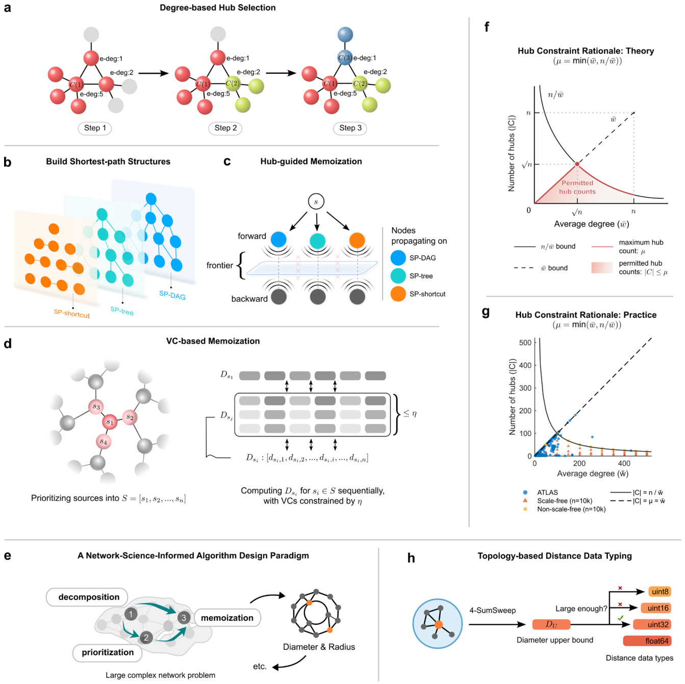
The degree-based prioritization enhances the effectiveness of vector comparison by making structurally influential nodes available earlier. It is easy to compute and we found that more complex measures (such as the sum or maximum of neighbor degrees) offer no significant efficiency improvements. Nonetheless, applying vector comparison unrestrictedly can potentially lead to O(n3) complexity in the worst case, as up to O(n2) comparisons can be involved, each requiring O(n) work. To mitigate this, CC-BFS imposes a constraint η on the maximum number of VC operations allowed per SSSP computation. We set , where is the network’s average node degree. This choice is derived from complexity optimization that balances graph traversal and vector comparison costs (details in Supplementary Note 2). This constrained VC-based memoization is a foundational component of CC-BFS that offers significant efficiency gains particularly in sparse networks. Building on this basic memoization strategy, we found that both highly heterogeneous and dense networks benefit from further network hierarchy exploitation, which leads to our next strategy: hub-guided memoization.
Hub-guided memoization for dense complex networks
While VC-based memoization is effective in sparse networks, its efficiency diminishes in networks with dense connectivity or complex SP patterns, topologies common in several domains among which are maritime networks [28] and online social platforms [29]. In these scenarios, the sheer number of alternative paths obscures the distance information captured by any single SP-tree, the O(n) cost per VC operation becomes prohibitive and offers little benefit. This limitation necessitates a more sophisticated strategy that can harness the deeper structural regularities inherent in dense complex networks.
CC-BFS addresses this challenge with a complementary hub-guided memoization strategy. This approach pivots from a global to a local reuse of information by selecting a small set of influential hub nodes and precomputing their associated hierarchical SP structures. For each selected hub s, CC-BFS constructs three specialized subgraphs from the original graph (Figure 1b), each designed for a specific computational purpose:
- SP-tree (Ts): A canonical tree representing one SP from hub s to all other nodes. It provides a lightweight structure for rapidly identifying nodes of interest at the next SP level. It keeps a memory of node hierarchy.
- SP-DAG (Γs): A directed acyclic graph (DAG) representing all SPs from hub s. It captures the complete SPs emanating from the hub, enabling efficient inter-level traversal for finding SPs exhibiting incremented distances from the hub. It keeps a memory of how nodes are connected along the shortest paths according to the node hierarchy.
- SP-shortcut (Hs): A subgraph of auxiliary edges connecting nodes at the same distance (SP level) from hub s. These shortcuts allow for efficient intra-level exploration, capturing paths that do not alter the distances from the hub. It keeps a memory of the connectivity redundancy that generates the same shortest path distances according to the node hierarchy.
These SP structures synergistically guide SSSP computations for hub-neighboring nodes (spoke nodes). When searching from a spoke node s with reference hub cs, the algorithm traverses corresponding parts of the hub’s SP structures in a proper order to progressively identify nodes at the target SP level. This hierarchical exploration drastically curtails edge examinations: instead of checking all O(|Adj(u)|) neighbors for each frontier node u (where Adj(u) is the adjacency list of u in the original graph, i.e., graph neighborhood, and a frontier node is a node one step closer to s than nodes at the target SP level), the algorithm inspects only edges within cs’s precomputed SP structures, which typically represent a small fraction of total adjacencies.
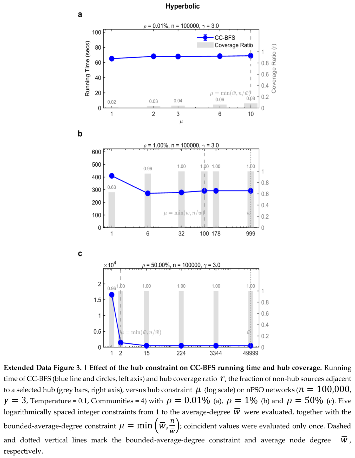
Constructing the SP structures for each hub involves an O(m) overhead, equivalent to executing a single-source BFS. To manage this overhead, CC-BFS employs a degree-based heuristic to select hub nodes based on their effective degrees at the time of selection (Figure 1a, SelectHubNodes in Procedure 3.1, Supplementary Note 1), with the objective of maximizing each hub’s coverage. Furthermore, we constrain the maximum number of hubs using the bounded-average-degree , where is average node degree and n is the number of nodes. This bounded formula for μ prevents excessive SP-structure construction in both sparse and dense connectivity regimes while retaining only influential hubs that actively participate in SP routing (Figure 1f; for detailed analysis, see Supplementary Note 3), and the practical effectiveness of this choice is supported by Extended Data Figure 3. Empirical evidence shows that this heuristic produces a sufficiently small hub set in negligible time, whereas finding the minimum hub set for full coverage (a minimum dominating set problem) is computationally demanding [30].
CC-BFS integrates the aforementioned strategies into a cohesive APSP solution: First, the algorithm selects at most μ hub nodes using SelectHubNodes. Then, for each hub s, it computes the SSSP distance vector Ds and the corresponding SP structures (Ts,Γs,Hs) (Figure 1b, BuildSPStructures in Procedure 3.2, Supplementary Note 1). Next, it prioritizes the remaining nodes in descending order of their degrees and partitions them into two disjoint categories: spoke nodes, which are adjacent to at least one hub (with the highest-degree neighboring hub serving as the reference hub); and peripheral nodes, which are neither hubs nor spokes. The algorithm then computes the SSSPs for all remaining source nodes according to this prioritized order:
- Peripheral nodes: Processed using MemoizedSSS, which employs only VC-based memoization.
HubGuidedSSS also uses direction-adaptive propagation analogous to the direction switching mechanism of DO-BFS [5]. At each level, it switches between forward traversal of the hub’s SP structures and backward traversal of candidate nodes’ graph neighborhoods according to estimated edge-examination costs. This avoids redundant edge traversal when edges are non-uniformly distributed. We detail the step-by-step description of CC-BFS in the Methods section, along with its pseudocode in Supplementary Note 1 and correctness proof in Supplementary Note 6.
This sophisticated interplay of decomposition, prioritization, and memoization endows CC-BFS with superior scalability. To formally characterize this, we analyze its average-case time complexity under a simplified configuration model (see Supplementary Note 4), which preserves the first-order effects of degree heterogeneity, hub coverage and edge density while randomizing higher-order structure. This provides a tractable null model for isolating the contribution of information reuse (memoization) without relying on specific network properties. We define an average hub-coverage ratio, , where B is the set of spokes (hub-neighboring nodes) and is the degree of the reference hub cs for a spoke s ∈ B. With this, we show that the average-case running time of CC-BFS is bounded by . Here, the mn(1 − α) term accounts for traversing SP structures, while the term covers VC operations.
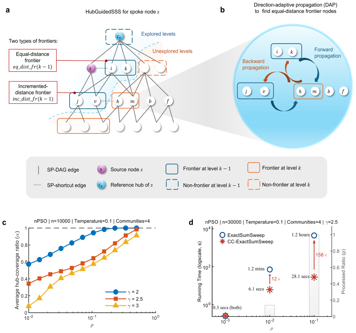
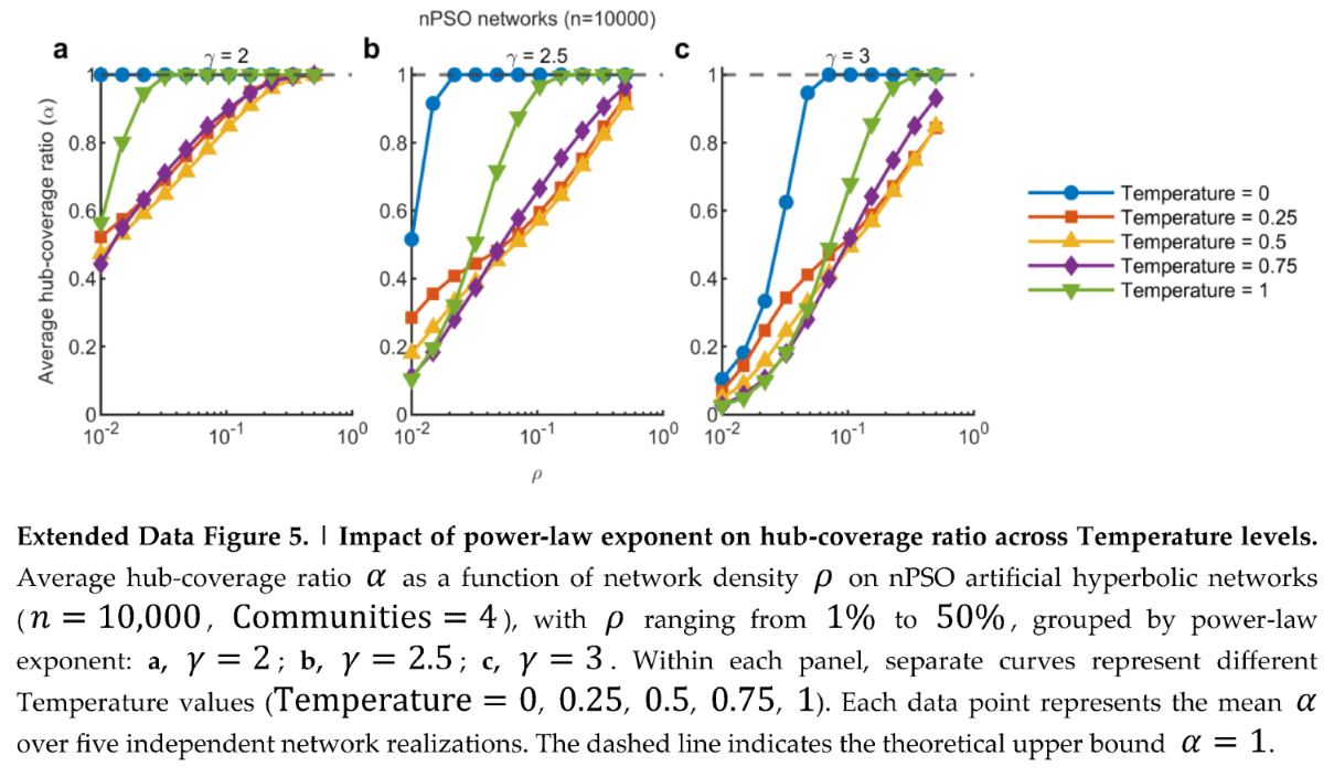
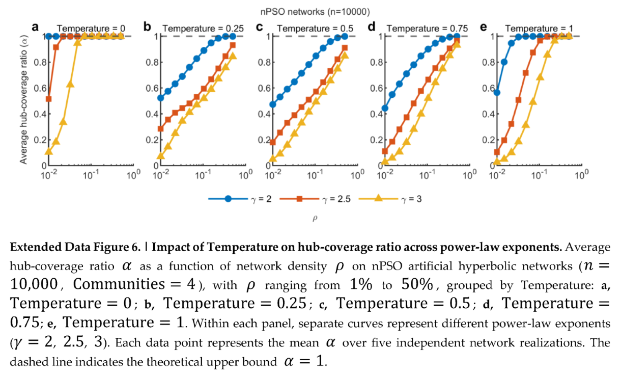
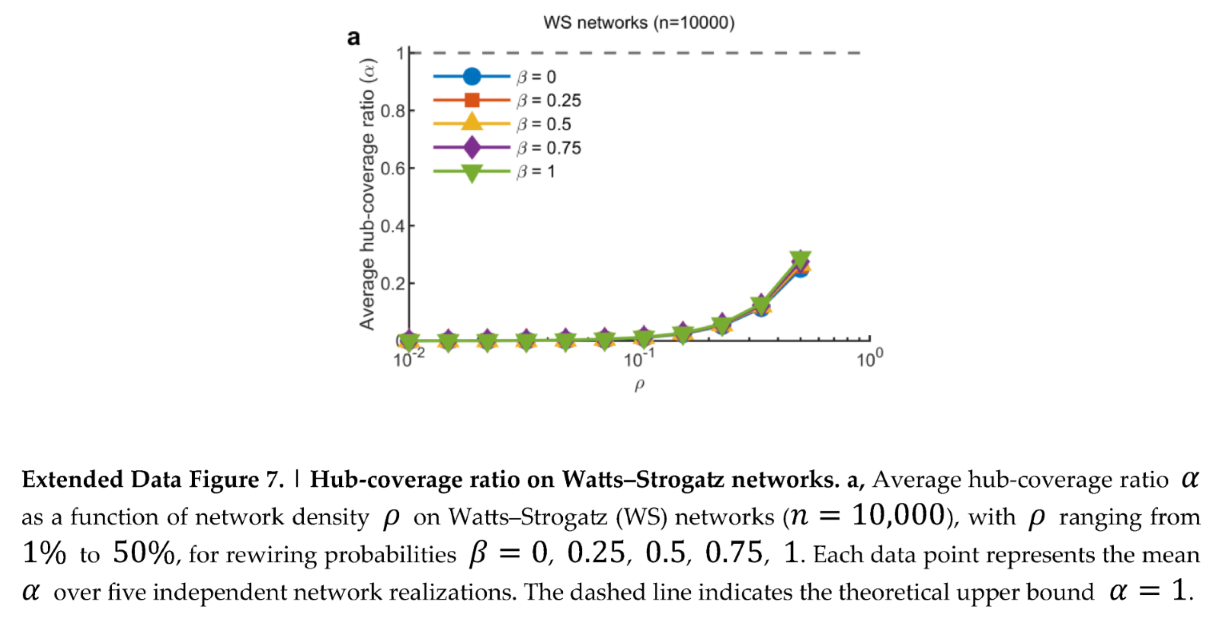
This bound reveals an ultra-small-world [2] advantage: in networks with dominant hubs (e.g., dense scale-free networks where the power-law exponent γ → 2), α approaches 1, which suppresses the mn(1 − α) term associated with traversing SP structures. To show this, we systematically characterized α across network conditions on the scale-free non-uniform popularity-similarity optimization (nPSO) networks [15,31] and the non-scale-free Watts-Strogatz (WS) networks [12] (Figure 4c and Extended Data Figure 5, Figure 6 and Figure 7; for detailed analysis, see Supplementary Note 9). Network density ρ and the power-law exponent γ are the dominant factors: α saturates near 1 for highly scale-free (γ = 2) and dense (ρ ≥ 0.1) networks, empirically confirming the α → 1 condition in the ultra-small-world regime. By contrast, WS networks maintained relatively low α across rewiring probabilities and densities, indicating that dense connectivity or small-world structure alone is insufficient; high hub coverage requires hub-dominated degree heterogeneity, as produced by scale-free organization. In this ultra-small-world regime triggered by scale-free topology, the running time is dominated by the remaining term , which is asymptotically smaller than the O(mn) baseline. Especially for dense networks where m~n2, this yields for CC-BFS, representing a substantial improvement over the O(n3) scaling of ZM-BFS and DO-BFS under the same density regime (see Table 1 for comparison). This theoretical finding is confirmed by our empirical evaluations reported in the performance benchmark section below.
Topology-based distance data typing
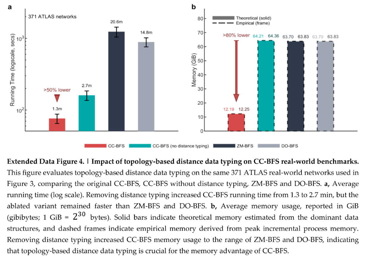
Beyond reducing computation time, CC-BFS also alleviates the memory bottleneck inherent to APSP. Standard implementations typically store the distance matrix in a fixed 64-bit type (e.g., uint64 or float64), which over-allocates memory for real-world small-world networks whose diameters remain modest. To address this, CC-BFS introduces a topology-based distance data typing strategy (Figure 1h): it first computes a strict upper bound on the network diameter using 4-SumSweep [32], then allocates the distance matrix with the smallest sufficient data type. This lossless memory optimization preserves exact shortest-path distances while reducing the memory footprint, often by a factor of 4 to 8 relative to standard 64-bit storage. To the best of our knowledge, existing exact APSP methods have not reported a similar strategy to optimize memory usage. CC-BFS remarkably outperforms other competitors also in absence of this data typing (Extended Data Figure 4), which further enhances its running time and memory saving.
Parallelizing CC-BFS
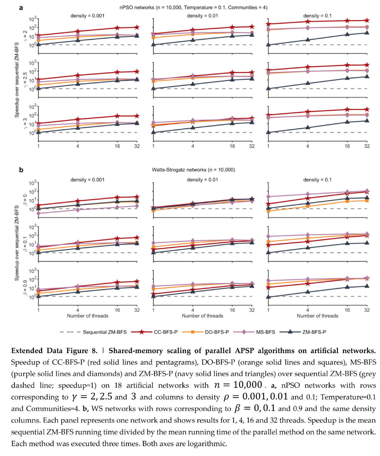
To make CC-BFS practical on modern multicore systems, we developed CC-BFS-P, a shared-memory parallel implementation that preserves both hub-guided and VC-based memoization. CC-BFS-P first constructs the independent hub structures in parallel and then processes the remaining, mutually dependent sources in synchronized batches, making completed distance vectors available between batches. In this way, parallelism is applied after much of the redundant graph traversal has already been removed. The full algorithm is presented in Algorithm 4 and analyzed in the Methods and Supplementary Note 7. Benchmarks demonstrated substantial practical speed advantages over competing parallel APSP algorithms across a range of network topologies (Extended Data Figure 8 and Figure 9), as discussed below.
Artificial and real-world benchmarks
We benchmarked three sequential APSP algorithms: ZM-BFS, the state-of-the-art DO-BFS and the proposed CC-BFS. We also compared CC-BFS-P with three competitive shared-memory parallel APSP algorithms: parallel ZM-BFS (ZM-BFS-P) [33], parallel DO-BFS (DO-BFS-P) [34] and multi-source BFS (MS-BFS) [35]. All benchmarks used unweighted, undirected networks, spanning both artificial networks with controlled structural parameters and real-world networks; the detailed setup is provided in the Methods.
Artificial scale-free networks with local clustering and communities
Hyperbolic scale-free networks [36], characterized by local node clustering, by power-law degree distributions P(k)∼k−γ, (where P(k) is the probability of node degree k and 2 < γ < 3) [13] and by small-world (for γ = 3, the average path length scales as logn) [37] or ultra-small-world properties (for γ → 2, the average path length scales as loglogn) [38], are prevalent in many complex network systems [14,39]. Their inherent hierarchical structure is well-suited for algorithms like CC-BFS that exploit hierarchical shortest-path (SP) structures. We employed the non-uniform popularity-similarity optimization (nPSO) model [15,31] to generate realistic hyperbolic networks, tuning parameters such as the power-law exponent γ (controlling scale-freeness), temperature (controlling clustering level), the number of communities, and connectivity density ρ.
Scalability with structural properties. We generated large networks (n = 100,000 nodes) with the nPSO model to analyze algorithm running time against key structural properties by varying one parameter at a time (Figure 2). CC-BFS consistently outperformed its competitors especially in highly power-law networks (Figure 2a). As γ increases (networks become less power-law Figure 2a), CC-BFS’s running time increased modestly but still substantially outperformed its competitors. Across different clustering levels (varied by Temperature, Figure 2b), CC-BFS again achieved significant efficiency boosts (on average approximately 14× over DO-BFS and 2400× over ZM-BFS), showing a non-monotonic trend with slight degradation at intermediate clustering, but performance improved when clustering continued decreasing (Temperature =0.9) due to effective VC-based memoization. Regarding network density ρ (Figure 2c), the running time of ZM-BFS increases linearly as expected. Interestingly, the running times of CC-BFS and DO-BFS remained relatively stable until certain density levels. Overall, CC-BFS retained a marked speed advantage owing to its network-science informed dynamic programming design for SP structure reuse. Increasing the number of communities (Figure 2d) generally enhanced CC-BFS performance as network modularity increased. Overall, CC-BFS achieved 40× to 2500× speedups over ZM-BFS and approximately 11× over DO-BFS on average.
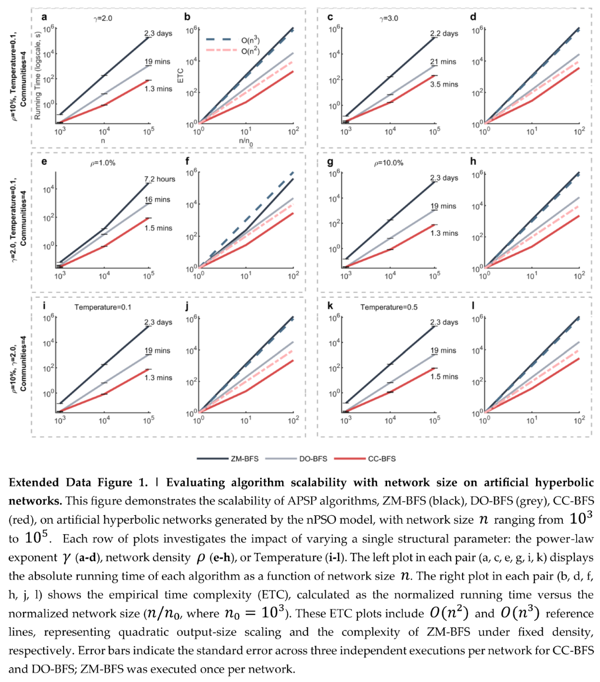
Scalability with network size. We examined how the algorithms scale with network size n, the most critical factor in practical scenarios. To do this, we generated artificial networks with different sizes (from 1,000 to 100,000) and other representative parameters, including γ and Temperature. Our empirical time complexity (ETC) analysis (Extended Data Figure 1, right plots in each pair, derived from running time curves in Extended Data Figure 1, left plots in each pair) showed that CC-BFS scales close to the quadratic lower bound of O(n2). In contrast, ZM-BFS scales nearly as O(n3) (or equivalently O(mn) for graphs with fixed density where m∝n2), while DO-BFS fell in between. These findings suggest CC-BFS offers a remarkable speedup over ZM-BFS and DO-BFS, making it more efficient for processing large-scale networks.
Scale-freeness helps but is not indispensable
CC-BFS exploits hierarchical shortest-path (SP) structures and therefore benefits strongly from the scale-free power-law degree heterogeneity and community organization present in nPSO networks. To stress-test the algorithm under a more adverse setting, we additionally benchmarked the algorithms on Watts-Strogatz (WS) networks [12], which can retain small-world structure and clustering but do not include both the scale-free hierarchy and the community hierarchy. This benchmark therefore probes how CC-BFS performs after these two favorable hierarchical layers are stripped away.
The results (Figure 2e,f) show that these hierarchies are important for the largest gains, but not necessary for performance improvement. Despite the absence of these two hierarchical properties, CC-BFS can still exploit network sparsity and small-world structure through complementary hub-guided and VC-based memoization. Finally, to assess the true impact of CC-BFS on real applications, we evaluated its performance on a large ATLAS of real-world networks.
Real-world networks
As an additional resource contribution, we expanded and made publicly available https://www.dropbox.com/scl/fi/owtzfdtegcuesaux1dmyj/ATLAS_extended.zip?rlkey=07pukzjasvc2hkafgl5kukw7u&st=srr82jrr&dl=0 the ATLAS dataset, increasing the 1,269-network, 14-class ATLAS benchmark of Zhao et al. [40] to 1,842 real-world networks spanning 35 classes (Supplementary Table 2). This broader dataset covers diverse biological, social, technological, transportation and information networks, making it a stringent benchmark for assessing algorithmic generalizability across network topologies. From this dataset, we employed 371 networks with sizes ranging from 10,000 to approximately 370,000 nodes to benchmark the empirical running times and scalability of the APSP algorithms.
CC-BFS was markedly faster than DO-BFS and ZM-BFS across nearly all size and density ranges, while CC-BFS-P (32 threads) achieved a further average speedup of around 11× over CC-BFS (Figure 3a-f). Network-by-network comparisons (Figure 3g,h) show that CC-BFS outperformed ZM-BFS on every ATLAS network, with a mean speedup of around 15×, with the advantage widening as network size increased. On two larger real-world networks of around one million nodes, CC-BFS-P completed com-YouTube and web-Google in 6.4 and 22.4 min respectively, compared with 1.8 and 6.1 h for CC-BFS and around two days for ZM-BFS (Figure 3i).
Figure 3.
| Benchmarking on real-world networks. Panels a–f compare the running times of ZM-BFS (black), DO-BFS (grey), CC-BFS (light red) and CC-BFS-P (32 threads; dark red) on real-world networks. Panels a–h and j use 371 ATLAS networks with size n ranging from 10,000 to approximately 370,000. Each algorithm was executed once per network. a-c, Running time (log-scale) versus network density ρ for networks grouped by size: a, small sizes (n ∈ [10k,50k)); b, medium sizes (n ∈ [50k,100k)); c, large sizes (n ≥ 100k). d-f, Running time (log-scale) versus network size n for networks grouped by density: d, low densities (ρ ∈ [0,0.0005)); e, medium densities (ρ ∈ [0.0005,0.003)); f, high densities (ρ ≥ 0.003). Each panel in a-f includes running-time moving-average curves and an inset bar plot showing average running times within the corresponding group; shaded bands denote local standard error of running times. g-h, Comparison of the running time of CC-BFS (x-axis) and ZM-BFS (y-axis) on log-log scatter plots, where each point represents one ATLAS network. The red dashed line represents y = x; points above this line indicate CC-BFS is faster. g, Points are colored by network density. h, Points are colored by network size. i, Running-time comparison of CC-BFS, DO-BFS, ZM-BFS and CC-BFS-P (32 threads) on two larger real-world networks, com-YouTube and web-Google. j, Memory usage comparison across all tested ATLAS networks, reported in GiB (gibibytes; 1 GiB = 230 bytes). Solid bars indicate theoretical memory estimated from the dominant data structures. Dashed frames indicate empirical memory derived from peak incremental process memory. The shared annotation indicates that CC-BFS and CC-BFS-P both required over 80% less memory than DO-BFS and ZM-BFS.
Figure 3.
| Benchmarking on real-world networks. Panels a–f compare the running times of ZM-BFS (black), DO-BFS (grey), CC-BFS (light red) and CC-BFS-P (32 threads; dark red) on real-world networks. Panels a–h and j use 371 ATLAS networks with size n ranging from 10,000 to approximately 370,000. Each algorithm was executed once per network. a-c, Running time (log-scale) versus network density ρ for networks grouped by size: a, small sizes (n ∈ [10k,50k)); b, medium sizes (n ∈ [50k,100k)); c, large sizes (n ≥ 100k). d-f, Running time (log-scale) versus network size n for networks grouped by density: d, low densities (ρ ∈ [0,0.0005)); e, medium densities (ρ ∈ [0.0005,0.003)); f, high densities (ρ ≥ 0.003). Each panel in a-f includes running-time moving-average curves and an inset bar plot showing average running times within the corresponding group; shaded bands denote local standard error of running times. g-h, Comparison of the running time of CC-BFS (x-axis) and ZM-BFS (y-axis) on log-log scatter plots, where each point represents one ATLAS network. The red dashed line represents y = x; points above this line indicate CC-BFS is faster. g, Points are colored by network density. h, Points are colored by network size. i, Running-time comparison of CC-BFS, DO-BFS, ZM-BFS and CC-BFS-P (32 threads) on two larger real-world networks, com-YouTube and web-Google. j, Memory usage comparison across all tested ATLAS networks, reported in GiB (gibibytes; 1 GiB = 230 bytes). Solid bars indicate theoretical memory estimated from the dominant data structures. Dashed frames indicate empirical memory derived from peak incremental process memory. The shared annotation indicates that CC-BFS and CC-BFS-P both required over 80% less memory than DO-BFS and ZM-BFS.
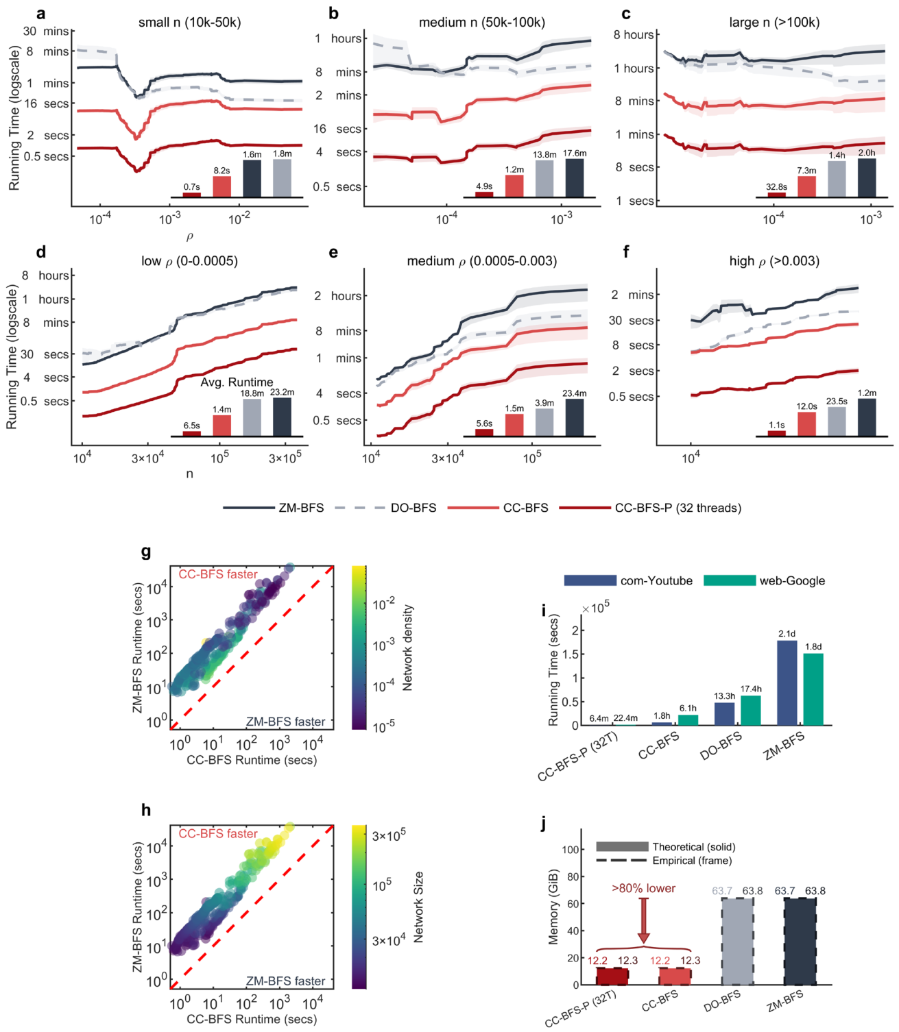
We also evaluated memory usage across all tested ATLAS real-world networks (Figure 3j). The theoretical memory was estimated from the dominant data structures of each algorithm, including the distance matrix for all methods and, for CC-BFS, also the SP-DAGs, SP-shortcuts and SP-trees. This estimate closely matched the empirical peak incremental process memory, showing that the theoretical approximation is accurate. Overall, CC-BFS and CC-BFS-P required over 80% less memory than DO-BFS and ZM-BFS owing to their topology-based distance data typing strategy.
Parallelization amplifies efficiency
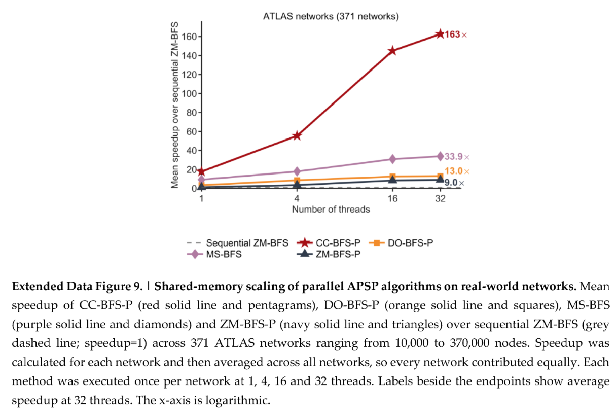
Reducing algorithmic work before distributing it across cores proved more effective than parallelizing BFS alone. By retaining memoization, CC-BFS-P gives each worker substantially fewer edges to traverse. At 32 threads, it substantially accelerates the sequential CC-BFS across the 100,000-node networks in Figure 2. Across the 18 networks used for thread-scaling analysis, CC-BFS-P achieved an average speedup of around 140× over sequential ZM-BFS, compared with around 49× for MS-BFS, 45× for DO-BFS-P and 14× for ZM-BFS-P (Extended Data Figure 8). CC-BFS-P led on all nine nPSO networks and five of nine Watts–Strogatz networks, whereas MS-BFS led on the remaining four. Across the same 371 ATLAS networks used in Figure 3, CC-BFS-P exhibited the same superior parallel scalability and outperformed its competitors by a huge margin (Extended Data Figure 9).
Ablation of CC-BFS components
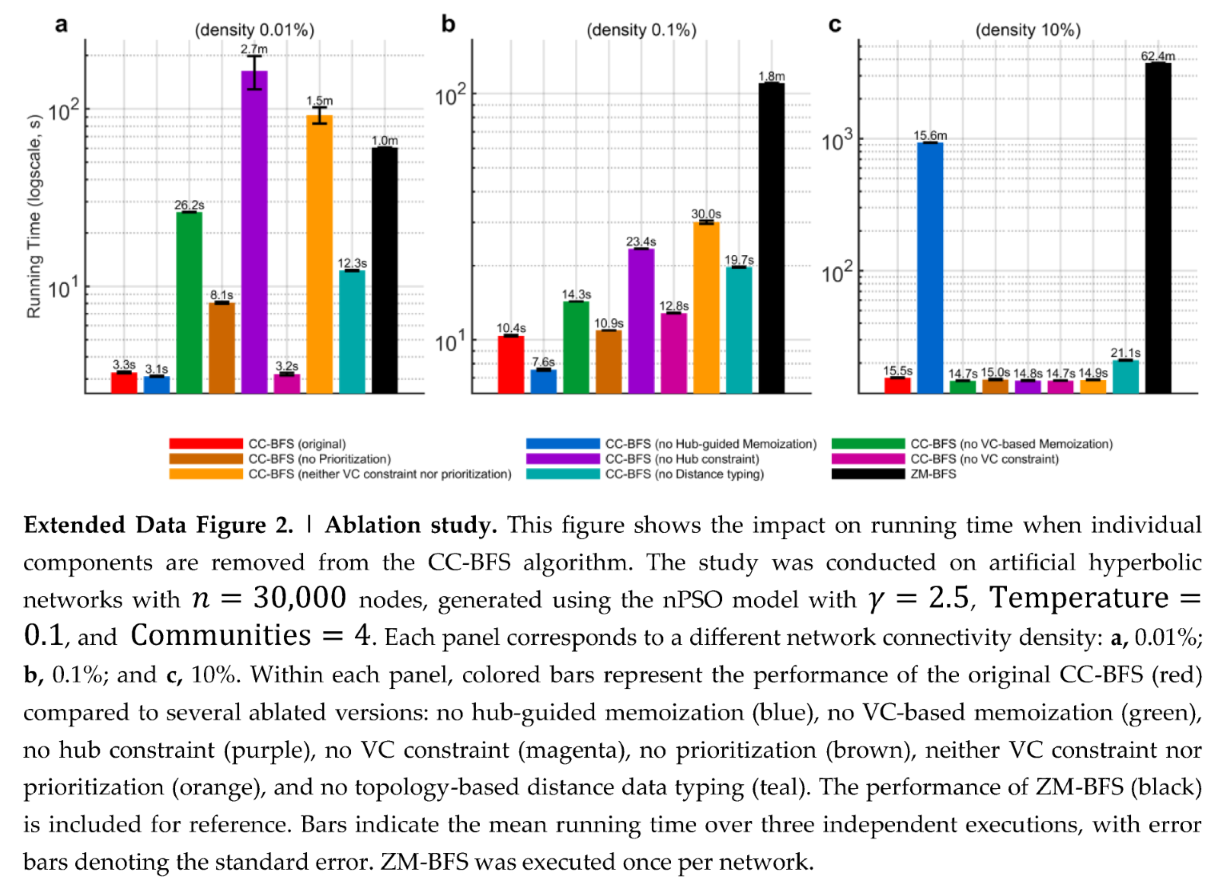
To isolate the contribution of each design choice in CC-BFS, we selectively disabled individual components and benchmarked the resulting variants on artificial networks with 30,000 nodes across densities from 0.01% to 10% (Extended Data Figure 2). The ablation results show that VC-based memoization is most important in sparse regimes, whereas hub-guided memoization becomes dominant in dense regimes; prioritization and the hub and VC constraints further stabilize performance. The full CC-BFS algorithm remained best or near-best across settings. The ATLAS ablation (Extended Data Figure 4) further showed that topology-based distance data typing (selecting the smallest distance data type based on network diameter) primarily accounts for the memory advantage of CC-BFS. Removing it increased memory usage to the range of DO-BFS and ZM-BFS, while the ablated variant remained substantially faster than both baselines (see Supplementary Note 8 for detailed analysis).
Generalization to diameter and radius
The network science principles underpinning CC-BFS extend beyond APSP to other multi-source shortest path problems. We demonstrate this by applying them to exact network diameter and radius computation. Although state-of-the-art methods [32,41] already reduce the cost relative to n independent BFS runs, they still treat the underlying SSSP computations largely as separate searches and do not explicitly reuse information across sources. CC-ExactSumSweep mitigates this limitation by enhancing ExactSumSweep [32], currently the fastest exact method for unweighted graphs, with CC-BFS-style reuse of SP information. On artificial hyperbolic networks (Figure 4d), CC-ExactSumSweep markedly outperformed ExactSumSweep as network density ρ increased (ρ ≥ 1%), confirming that CC-BFS’s core strategies generalize effectively to multi-source unweighted shortest path problems.
Figure 4.
| Hub-guided search mechanism, hub-coverage characterization, and generalization to diameter and radius computation. a, Illustration of the hub-guided single-source search (HubGuidedSSS) procedure for a spoke source node s with reference hub cs. The level-by-level search from s partitions frontier nodes at level k − 1 into two frontiers: the equal-distance frontier eq_dist_fr(k − 1) and the incremented-distance frontier inc_dist_fr(k − 1), which are used to discover nodes at the next unexplored level k by traversing the precomputed SP structures of the hub. Levels with depths <k are already explored and non-frontier nodes were settled via VC (e.g., using the distance vector of cs). b, Detailed view of the direction-adaptive propagation (DAP) used to find equal-distance frontier nodes at level k. The algorithm dynamically chooses between forward propagation, which traverses SP structure edges from the frontier nodes, and backward propagation, which traverses graph edges from candidate nodes at the next level. c, Average hub-coverage ratio α as a function of network density ρ on nPSO networks (n = 10,000, Temperature = 0.1, Communities = 4), with ρ ranging from 1% to 50%, for power-law exponents γ = 2, 2.5, and 3. The dashed line indicates the theoretical upper bound α = 1. Each data point represents the mean α over five independent network realizations. d, Running time comparison of network diameter and radius algorithms, CC-ExactSumSweep and ExactSumSweep, on nPSO networks (n = 30,000, γ = 2.5, Temperature = 0.1, Communities = 4), with network density ρ ranging from 0.1% to 10%. Running times are shown on the left y-axis (log scale), with ExactSumSweep shown as blue circles and CC-ExactSumSweep as red asterisks. Each point represents the average running time over three independent executions per network. Grey bars and the right y-axis show the processed ratio p, defined as the fraction of nodes for which SSSP distances were computed relative to the total number of nodes. Error bars are omitted for clarity.
Figure 4.
| Hub-guided search mechanism, hub-coverage characterization, and generalization to diameter and radius computation. a, Illustration of the hub-guided single-source search (HubGuidedSSS) procedure for a spoke source node s with reference hub cs. The level-by-level search from s partitions frontier nodes at level k − 1 into two frontiers: the equal-distance frontier eq_dist_fr(k − 1) and the incremented-distance frontier inc_dist_fr(k − 1), which are used to discover nodes at the next unexplored level k by traversing the precomputed SP structures of the hub. Levels with depths <k are already explored and non-frontier nodes were settled via VC (e.g., using the distance vector of cs). b, Detailed view of the direction-adaptive propagation (DAP) used to find equal-distance frontier nodes at level k. The algorithm dynamically chooses between forward propagation, which traverses SP structure edges from the frontier nodes, and backward propagation, which traverses graph edges from candidate nodes at the next level. c, Average hub-coverage ratio α as a function of network density ρ on nPSO networks (n = 10,000, Temperature = 0.1, Communities = 4), with ρ ranging from 1% to 50%, for power-law exponents γ = 2, 2.5, and 3. The dashed line indicates the theoretical upper bound α = 1. Each data point represents the mean α over five independent network realizations. d, Running time comparison of network diameter and radius algorithms, CC-ExactSumSweep and ExactSumSweep, on nPSO networks (n = 30,000, γ = 2.5, Temperature = 0.1, Communities = 4), with network density ρ ranging from 0.1% to 10%. Running times are shown on the left y-axis (log scale), with ExactSumSweep shown as blue circles and CC-ExactSumSweep as red asterisks. Each point represents the average running time over three independent executions per network. Grey bars and the right y-axis show the processed ratio p, defined as the fraction of nodes for which SSSP distances were computed relative to the total number of nodes. Error bars are omitted for clarity.
Discussion
Our findings show that CC-BFS substantially accelerates all-pairs shortest path (APSP) computation for unweighted graphs in many real-world networks with hierarchical structures, outperforming both ZM-BFS and DO-BFS. This addresses the practical O(mn)~O(n3)—in dense networks m~n2 with n number of nodes, m number of edges—scalability bottleneck of unweighted APSP through network-science-informed algorithm design.
The memoization strategies in CC-BFS are fundamentally rooted in dynamic programming and distinguish it from standard BFS; hence, we characterize CC-BFS as a dynamic programming variant of BFS. In contrast, ZM-BFS and its variant DO-BFS perform independent single-source search iterations with no inter-iteration information sharing; thus, their average-case time complexities are bounded by O(mn). CC-BFS transcends this limitation by strategically decomposing the APSP problem around influential hubs and memoizing their associated SP structures (SP-trees, SP-DAGs, and SP-shortcuts), which serve as meta-information about the network’s geodesic landscape [42,43], echoing the distance-backbone concept for weighted networks [44]. This hierarchical reuse, augmented by VC-based memoization, drastically prunes redundant explorations and yields the improved average-case time complexity , where α is the average hub-coverage ratio. This time complexity for ultra-small-world and dense networks can be approximated by O(n2.5) which significantly improves O(n3) for ZM-BFS and DO-BFS. Hence, the resulting advantage is especially strong in heterogeneous degree networks with scale-free topology, where hubs contribute disproportionately to shortest-path organization [45]. In WS networks, both CC-BFS and DO-BFS benefit from small-world structure, but CC-BFS remains more robust as clustering and path length increase. Finally, in our tests we show that the running time advantage of CC-BFS on DO-BFS and ZM-BFS remains consistent regardless of the usage of the topology-based distance data typing, which instead is crucial for the memory advantage of CC-BFS.
CC-BFS has notable strengths but also limitations. It is currently designed for unweighted, undirected graphs, and extending its memoization strategies to weighted and directed graphs remains an open problem. Hub-guided memoization is most effective in heterogeneous scale-free networks, although CC-BFS remains competitive when this hierarchy is less prominent. Importantly, the reduction in graph traversal makes CC-BFS particularly well suited to shared-memory parallelization, because graph traversal is typically limited by irregular memory access; a smaller traversal workload therefore places less pressure on shared memory bandwidth and caches as workers are added. As a result, CC-BFS-P showed strong multicore scaling and delivered the highest speedups on most networks tested. It reduced hour- or day-scale computations to minutes, making exact APSP practical on ordinary multicore systems. Further gains may be possible by adapting the batch size to network structure and hardware (Supplementary Note 7).
The hub-centric idea of CC-BFS is reminiscent of the remarkable information transmission efficiency observed in complex biological systems, such as the brain. While these analogies are not meant for direct biological mimicry [9,10,46,47], we believe that insights from biological systems and network science advancements are an important direction to explore for algorithmic innovation [9,10].
CC-BFS promotes a network-science-informed dynamic programming paradigm for algorithm design based on problem decomposition, prioritization, and memoization, which act synergistically to reuse intermediate results efficiently across structurally distinct subproblems (Figure 1e). As a further step, we’ve already applied CC-BFS and the same underlying paradigm to develop new algorithms [48] for the efficient computation of betweenness centrality [1] and congruence [2] measures, helping redefine the frontiers of large-scale network analysis. Our next step is a distributed-memory implementation of CC-BFS for supercomputers, which would remove the runtime and memory limits of a single machine. With it, we aim to compute exact APSP on the largest networks for which it has ever been computed.
Methods
The APSP problem and SP structures
In this subsection, we introduce the fundamental concepts and notation for APSP and related SP structures. Given an unweighted and undirected graph G = (V,E) with a single connected component, the general SP problem asks to find the SP between each given pair of nodes. Let V(G) and E(G) denote the set of nodes and edges in G, respectively, with n = |V| nodes and m = |E| edges. The SP distance from node i ∈ V to j ∈ V is denoted by di,j. We use Adj(i) = {j ∈ V∣(i,j) ∈ E} to represent the adjacency list of i, and wi = |Adj(i)| the degree of i. The eccentricity ecci of a node i ∈ V is defined as the maximum SP distance from i to any other node in the network:
Two network properties derived from eccentricity are the diameter diam(G) and radius rad(G), respectively defined as and . We use to denote an arbitrary path from node i to node j, where v1,v2,…,vk−1 are the intermediate nodes. The length of a path is the number of edges it contains, i.e., . The SP between two nodes, Pi→j, is a path with the minimum possible length, so that . We denote the SP distance by di,j = l(Pi→j), and V(Pi→j) denotes the set of nodes in path Pi→j. By definition, we let Pi→i=⟨i⟩. Furthermore, Pi→x∘Px→j denotes the concatenation of two paths. If x ∈ V(Pi→j), then the concatenated path is also a valid SP from i to j.
The all-pairs shortest path (APSP) problem asks to find an SP between all node pairs. It can be interpreted in two ways: (1) Computing for each node pair (i,j) the SP distance between them. This is known as the distance version of the APSP problem [19,49], in which case the output is an n × n distance matrix . (2) Finding for each node pair (i,j) a representative SP Pi→j. This is also referred to as the SP-tree problem [50], where the goal is to construct an SP-tree rooted at each node. This article primarily addresses the distance version, but the proposed method (CC-BFS) could be extended to compute path representatives without increased complexity (see Supplementary Table 1 for notation and terminology).
Beyond the graph itself, we consider three SP structures for efficient path-finding: SP-tree, SP directed acyclic graph (SP-DAG), and SP-shortcut. We denote the SP-tree rooted at i ∈ V by Ti. An SP-tree is a subgraph of the original graph containing exactly one SP between the root i and every other node. For a given node v, its neighborhood in Ti is:
An SP-tree organizes nodes hierarchically into different SP levels (or BFS levels); the k-th SP level for a source node i is denoted by Li(k). While an SP-tree provides a compact representation of single-source SPs, it is insufficient for representing all possible SPs. To address this, we introduce the SP-DAG, denoted by Γi for a root i ∈ V. The SP-DAG [1] is a subgraph of G containing all edges (v,j) ∈ E that lie on any SP from i. For a given v, its neighborhood in Γi is:
Both SP-trees and SP-DAGs encode hierarchical single-source SP information. However, while Ti is a tree in the formal sense, Γi is not, as a node may have multiple parents. Unlike an SP-tree, which may not be unique if multiple SPs exist between nodes, the SP-DAG is always unique as it encompasses the complete set of SPs from the root.
An SP-DAG captures the inter-level links of an SP-tree. Additionally, we introduce a third structure, SP-shortcut (denoted by Hi for node i), which captures the intra-level links of an SP-tree. Its neighborhood is defined as:
SP-shortcuts complement SP-DAGs and SP-trees to form a comprehensive roadmap for efficient path-finding in CC-BFS. Figure 1b provides illustrative examples of an SP-shortcut Hi, an SP-tree Ti, and an SP-DAG Γi, all rooted at node i. In general, SP-trees exhibit much sparser connectivity compared to their SP-DAG counterparts, and Ti ⊆ Γi ⊆ G holds.
In the following sections, we elaborate on the CC-BFS algorithm proposed in this article, which emphasizes a hybrid graph traversal strategy via the aforementioned three SP structures.
ZM-BFS
ZM-BFS refers to the BFS-based algorithm for computing all-pairs shortest paths (APSP) in unweighted networks G = (V,E). The canonical single-source BFS starts from a given source node s ∈ V and computes the SSSP via pure graph traversal. During this process, nodes transition through three states: undiscovered, discovered (queued for visiting), and visited. Initially, only s is marked as discovered. At each iteration, the algorithm visits all discovered nodes (i.e., nodes in the current frontier, not yet visited) by examining their graph neighbors and labeling their undiscovered neighbors as discovered, after which the previously discovered nodes are labeled as visited. This continues until all nodes are discovered. To compute APSP, ZM-BFS simply executes the single-source BFS from every source s ∈ V. The full procedure for ZM-BFS is detailed in Algorithm 1, Supplementary Note 1. For more information, see Cormen et al. [51].
The single-source BFS runs in O(n + m) time for visiting n nodes and examining m edges. For the APSP problem, ZM-BFS repeatedly calls the single-source BFS from a different source s ∈ V each time. This leads to an overall average- and worst-case time complexity of O(nm + n2) = O(nm) (since m ≥ n − 1 for connected graphs), which depends only on n and m rather than higher-order graph topology. The space complexity is O(n2) for storing the APSP distance matrix.
DO-BFS
DO-BFS (direction-optimizing BFS) is a variant of BFS that combines the standard top-down approach with a bottom-up approach to reduce redundant edge examinations [5]. In a top-down step (as in classical BFS), each node in the current frontier checks all its outgoing neighbors to find undiscovered children. In a bottom-up step, this process is inverted: each undiscovered node checks its neighbors to see if any are in the current frontier (i.e., if there is a valid parent in the SP-tree) before labeling itself discovered. By switching between the top-down and bottom-up approaches when appropriate, DO-BFS avoids examining many edges that would have been checked in a purely top-down approach. This yields potentially far fewer edge inspections in networks with small-world topology, where the frontier can encompass a large fraction of all nodes. The algorithm is detailed in Algorithm 2, Supplementary Note 1.
At each SP level, DO-BFS dynamically chooses the search direction (top-down or bottom-up) using a simple online heuristic based on frontier size and remaining unexamined edges. Intuitively, if continuing in top-down mode would require checking significantly more edges than the bottom-up alternative, the algorithm switches to the bottom-up mode. Formally, for a graph G = (V,E), where V is the node set and E is the edge set, let n = |V| and m = |E| denote the numbers of nodes and edges, respectively. Let nf be the number of nodes in the current frontier and let mf denote the number of edge examinations that a top-down step would perform (the sum of degrees of all frontier nodes). Let mu be the number of edge examinations required for a bottom-up step (i.e., the sum of degrees of all undiscovered nodes). DO-BFS initially starts a top-down search from the source. During the search, it triggers a direction switch once mf becomes much larger than mu (in practice, when for some tuning parameter αDO). This condition typically occurs when the frontier is large, occupying a substantial portion of the graph. Conversely, when the frontier size shrinks again (indicating the search has passed the dense middle levels), the algorithm switches back to the top-down mode for the remaining levels. A second threshold βDO is used to decide this reversal: when nf falls below (a small fraction of total nodes), bottom-up mode is no longer considered beneficial. In our benchmarks, for DO-BFS we used αDO = 14 and βDO = 24, the values selected in the original DO-BFS study [5]. To minimize switching overhead, the algorithm also changes the frontier representation for each mode: the top-down mode uses a queue to store frontier nodes, while the bottom-up mode uses a bitmask (or bitmap) for frontier representation to allow O(1) membership checking. Converting between these representations at each switch often incurs negligible cost compared to the savings in edge examinations.
The average-case time complexity of DO-BFS remains O(mn) for random graphs. In the worst case, however, DO-BFS may perform more work than ZM-BFS. This can occur in topologies like ring lattices, where a bottom-up step is not guaranteed to be cheaper than its top-down equivalent, potentially causing the algorithm to inspect more than mn edges overall. The space complexity is O(n2) for storing the APSP distance matrix.
CC-BFS
CC-BFS is a dynamic programming variant of BFS that integrates the network science principles of decomposition, prioritization and memoization to solve the APSP problem in unweighted graphs. The full algorithm is presented in Algorithm 3, Supplementary Note 1, and elaborated below.
Overview
CC-BFS proceeds in two stages. First, it selects a small set of influential hub nodes, C, whose SP structures are likely to cover a large fraction of all-pairs geodesics. These hubs are processed first: for each hub, the algorithm computes its SSSP distances and constructs its associated SP structures. The remaining non-hub nodes are then processed in descending order of degree. Specifically, spoke nodes (hub-neighboring nodes) perform a hub-guided SSS that reuses information from their reference hub. Peripheral nodes (remaining non-hub, non-spoke nodes) perform a memoized SSS that leverages only previously computed SSSP distance vectors. Throughout this process, CC-BFS maintains the SSSP distance vectors of all processed sources to accelerate subsequent computations, while preserving the source-by-source, level-by-level characteristic of classical ZM-BFS.
Select hub nodes
Given an unweighted, undirected graph G = (V,E) with n = |V| nodes and m = |E| edges, the SelectHubNodes procedure identifies a set of hub nodes C. It initializes an empty set C and computes the degree wi for each node i ∈ V as the initial effective degree. Initially, all nodes are marked as uncovered and unmasked. The algorithm iteratively selects a new hub node from the unmasked nodes with the highest effective degree, adds it to C, and marks its uncovered neighbors as covered. The effective degrees of all nodes are then updated by removing the degree contributions of the newly selected hub and its newly covered neighbors, therefore prioritizing nodes that are likely to cover more undiscovered regions of the network. The process repeats until all nodes are covered or the number of hubs reaches a predefined maximum (hub constraint), |C| = μ, where , with defining the average node degree; the resulting limit is rounded to the nearest integer in the implementation. This hub constraint formula is derived by the analysis of hub selection behavior across different network topologies (Supplementary Note 3), which shows that keeps the selected hub set small across connectivity regimes while preserving broad coverage. Its performance impact is further evaluated in Supplementary Note 5, where is compared with alternative hub constraints and is shown effective in all cases.
The greedy hub-selection heuristic runs in O(n + m + n|C|) time, which simplifies to O(m + n|C|) for a connected graph. We show in Figure 1f that the bounded constraint limits |C|, which prevents the construction of hub shortest-path structures from dominating the computation.
BuildSP structures
For each hub node s ∈ C, the BuildSPStructures procedure executes a BFS from s to compute its SSSP distance vector Ds while simultaneously constructing the following SP structures:
- SP-DAG (Γs) containing all SPs from s;
- SP-tree (Ts) providing a compact SP representation; and
- SP-shortcut (Hs) capturing intra-level connections.
In our implementation, we skip recording first-level edges in an SP-shortcut because these edges are never visited by HubGuidedSSS: the algorithm visits the SP-shortcut edges only from incremented-distance frontier nodes, and no such nodes exist at the first level (Figure 4a). The procedure also records SP levels Ls and the eccentricity eccs for each hub. These precomputed structures are used for accelerating SSSP computations for spoke nodes via HubGuidedSSS. As detailed in Procedure 3.2, constructing all SP structures for a source requires the same number of edge examinations as a standard BFS, keeping the complexity for processing each hub at O(m).
Hub-guidedSSS for spoke nodes
HubGuidedSSS computes the SSSP for spoke nodes utilizing both hub-guided memoization and VC-based memoization to drastically reduce redundant edge examinations. The core idea is that in many real-world networks, a few influential hubs lie on a disproportionate number of SPs, making them ideal reference points for pathfinding from their neighbors.
For a spoke source node s, the algorithm selects the highest-degree adjacent hub cs ∈ C as its reference. Every node v at distance k from s (denoted by v ∈ Ls(k)) can be categorized into one of two disjoint sets: either its SP from s passes through cs (i.e., ), or it does not (i.e., ). The algorithm settles the real SP distance of the reference hub cs and all nodes in the set via a single VC operation (comparing Ds and ). To identify the remaining set of nodes, HubGuidedSSS maintains two complementary frontiers for each level k (Figure 4a):
- Equal-distance frontier eq_dist_fr(k): the set of nodes at distance k from both s and cs;
- Incremented-distance frontier inc_dist_fr(k): the set of nodes at distance k from s but k + 1 from cs.
By construction, these two frontiers partition the set of nodes whose SPs from s do not pass through cs:
The search proceeds in rounds from k = 1 to eccs. The first level (k = 1) is handled specially: each neighbor t ∈ Adj(s)∖{cs} is assigned to either eq_dist_fr(1) or inc_dist_fr(1), and its distance is set to Ds[t] ← 1. For subsequent levels (k ≥ 2), HubGuidedSSS leverages the precomputed SP structures of cs to guide traversal for nodes in the two frontiers (i.e., hub-guided memoization):
- SP-tree traversal: For each node v ∈ eq_dist_fr(k − 1), traverse downward to retrieve its children at level k in . This step pre-identifies a subset of nodes for eq_dist_fr(k) at O(n) cost overall. Importantly, this traversal serves as an optimization when direction-adaptive propagation (elaborated below) is employed: by pre-populating candidate nodes in eq_dist_fr(k), it reduces the search space that backward propagation must examine (specifically, reducing the size of ). Consequently, SP-tree traversal is dispensable when the direction-adaptive propagation strategy is not used, as forward-only propagation can identify all necessary nodes through SP-DAG and SP-shortcut traversal.
- SP-DAG traversal: Each node v in both frontiers (eq_dist_fr(k − 1) ∪ inc_dist_fr(k − 1)) traverses the hub’s SP-DAG, . For each neighbor t of v in (where t is one level farther from cs), the algorithm attempts to relax the path to t through v. This step discovers SPs that span “vertically” relative to the hub’s SP levels.
- SP-shortcut traversal: Each node v ∈ inc_dist_fr(k − 1) is traversed along the hub’s shortcut structure, . For each shortcut edge connecting nodes at the same SP level from cs, the algorithm attempts to relax the path to t through v. This efficiently discovers SPs that span “horizontally” relative to the hub’s SP levels.
During this process, newly discovered nodes are assigned to the frontiers for the next level based on the aforementioned relationship. For instance, a node reached from eq_dist_fr(k − 1) (via or ) or from inc_dist_fr(k − 1) (via ) is placed into eq_dist_fr(k). A node reached from inc_dist_fr(k − 1) via is placed into inc_dist_fr(k). The search terminates when both frontiers are empty.
Besides hub-guided memoization, HubGuidedSSS employs two further optimizations:
- VC-based memoization: The algorithm can accelerate searches by reusing SSSP distance vectors from previously processed sources. This technique identifies SPs from the current source s that pass through an earlier source u by comparing their respective SSSP distance vectors. Specifically, if the search from s encounters a node u whose distance vector Du is already known, it performs a vector comparison (VC) operation:
This operation effectively merges u’s SP information into the tentative distance vector of s, avoiding redundant exploration of paths already investigated from u. To balance exploration and exploitation, VC is performed at most η times per source, where η is a tunable parameter. We derive the optimal constraint as
based on complexity minimization (Supplementary Note 2), where is the average network degree.
- 2.
- Direction-adaptive propagation: The aforementioned SP structure traversals propagate SPs in a forward direction, i.e., from depth k − 1 to k. To identify equal-distance frontier nodes at distance k (eq_dist_fr(k)) more efficiently, the algorithm dynamically switches between forward and backward propagation at each level by comparing estimated edge-examination cost (Figure 4b). In this direction choice, forward propagation explores the SP-DAG from eq_dist_fr(k − 1) and the SP-shortcut from inc_dist_fr(k − 1), while backward propagation starts from candidate nodes at the level k of the hub (i.e., , since ) and checks their incoming edges in the original graph G to find a parent in the previous frontiers. The forward cost fc(k) is the number of edges to be examined in this forward step:
To estimate the backward cost, we leverage the negative hypergeometric distribution [52]. Let be a population of candidate nodes around the objective level, and let N = |ξ(k)|. Let be the number of target nodes (successes) within this population. The expected number of draws from ξ(k) required to find one target node is given by . This value serves as a proxy for the search effort. The total backward cost bc(k) is the sum of costs for each node in the backward frontier, defined as
At each level, the algorithm chooses the direction with the lower estimated cost. This strategy, adapted from DO-BFS [5], is enhanced by using the SP level information to ensure each node is processed at most once per SSS, guaranteeing an O(m) worst-case bound for the traversal.
Essentially, HubGuidedSSS exploits network system heterogeneity by precomputing rich SP structures for a small set of hubs and then confining searches from spoke nodes largely to those structures, thus dramatically reducing the number of edges to be examined. Empirical evaluations show that this hub-guided search can reduce edge examinations by up to several orders of magnitude compared to ZM-BFS, with greater efficiency gains observed on larger and more degree-heterogeneous networks. Furthermore, since only a few hub nodes (often under 1% of V) undergo the full BFS, the time and space overhead for computing the SP structures remains manageable even for very sparse networks. Finally, the adaptive direction switching mechanism helps the algorithm adapt to varying connectivity patterns: at each step HubGuidedSSS automatically selects the most efficient search direction (forward or backward) for the region of the network being explored, contributing to its robust performance across diverse topologies. We prove the correctness of HubGuidedSSS in Supplementary Theorem 4, Supplementary Note 6.
Memoized SSS for peripheral nodes
For a peripheral source node s with no adjacent hub, CC-BFS uses MemoizedSSS to compute its SSSP. This procedure performs a BFS-like graph traversal while applying the same VC-based memoization described above, reusing distance vectors from up to η previously processed sources to avoid computing investigated SPs again. We prove the correctness of MemoizedSSS in Supplementary Theorem 3, Supplementary Note 6.
Topology-based distance data typing
To perform topology-based distance data typing, CC-BFS first computes an upper bound on the network diameter (Figure 1h). Specifically, it runs 4-SumSweep to obtain the eccentricity upper bound U[v] for each node v ∈ V, and then sets the diameter upper bound to DU = maxv∈VU[v]. Using this bound, the algorithm allocates the distance matrix with the smallest sufficient data type τ satisfying max(τ) ≥ 2DU. This requirement arises because DU is used as the initial distance value in CC-BFS, whereas VC-based memoization evaluates candidate path lengths of the form ds,u + du,v (equation (7)), where s is the current source, u is a previously processed source and v ∈ V; since both terms are bounded above by DU, the temporary candidate value can be as large as 2DU before the minimum update is applied. Accordingly, the implementation selects types such as uint8_t if 2DU ≤ 28 − 1, uint16_t if 2DU ≤ 216 − 1. Here, float64 serves as the default largest fallback type because it supports the IEEE 754 (+∞) representation and therefore avoids overflow during initialization and intermediate updates. This preprocessing step guarantees exact, overflow-free distance computation while avoiding unnecessary memory allocation.
Time complexity
The average-case time complexity of CC-BFS is (derived under a simplified configuration model, see Supplementary Note 4). Here, n = |V| and m = |E| denote the numbers of nodes and edges, respectively. The average hub-coverage ratio is bounded in (0,1), where B is the set of spoke nodes, cs ∈ C is the reference hub selected for a spoke source s, C is the set of selected hub nodes, and is the degree of cs. In this bound, mn(1 − α) accounts for the cost of traversing SP structures via hub-guided memoization, whereas captures the cost of VC-based memoization, under the optimal VC constraint , with denoting the average node degree. In the regime of ultra-small-world networks with dominant hubs (e.g., dense scale-free networks where the power-law exponent γ → 2), α → 1 and the SP structure traversal term mn(1 − α) is suppressed. In this regime, the running time is dominated by the remaining term , which is asymptotically smaller than the standard O(mn) baseline. For dense networks where m∼n2, this yields O(n2.5), a substantial improvement over the O(mn) = O(n3) scaling of ZM-BFS and DO-BFS under the same density regime (see Table 1 for comparison). We emphasize that this bound should be interpreted as an indicative average-case scaling rather than a strict worst-case guarantee, as its derivation relies on a simplified configuration model.
Space complexity
The space complexity of CC-BFS is O(n2) for storing the APSP distance matrix and SP structures of selected hub nodes, where n is the number of nodes. Topology-based distance data typing does not change this asymptotic complexity, but reduces the practical memory footprint by allocating the smallest sufficient distance data type.
CC-BFS-P
CC-BFS reduces exact APSP work through two complementary mechanisms: hub-guided memoization traverses precomputed shortest-path structures around selected hubs, whereas VC-based memoization reuses exact distance vectors from earlier sources. Only the latter creates dependencies between source searches. In CC-BFS-P, hub selection therefore remains sequential because it is greedy: selecting each hub changes the residual coverage scores that determine the next. Once the hub set C is fixed, the distance vectors and shortest-path structures of different hubs are independent and are constructed in parallel. The remaining n − |C| sources retain CC-BFS’s degree-descending priority and are partitioned into consecutive batches B1,…,BK of at most κP sources for P workers, with κ = 4. A persistent OpenMP team schedules sources dynamically within each batch to balance unequal search costs (Algorithm 4 and Supplementary Note 7).
During batch Bk, each search can reuse only distance vectors made available before that batch began. Every source writes to its own vector, and after all searches in the batch finish, their vectors become available together to subsequent batches. Delaying same-batch reuse can increase work but cannot alter the exact distances. We use κ = 4 to provide several tasks per worker for dynamic load balancing while amortizing synchronization; κ is tunable, and adapting it to the network and hardware may improve performance. Under the same simplified configuration model used for CC-BFS, and assuming balanced scheduling, the idealized average-case parallel time is . The first two terms describe sequential greedy hub selection, whereas the final term distributes the average CC-BFS search work across P workers. The bounded average-degree constraint gives and therefore). Reusable O(n) workspaces per worker add O(Pn) space, so total space remains O(n2) for a simple graph with P ≤ n. Unequal search costs, batch barriers and memory bandwidth limit ideal scaling; the full analysis is provided in Supplementary Note 7.
We compared CC-BFS-P with three shared-memory baselines. ZM-BFS-P distributes the independent source searches of textbook ZM-BFS across threads [33]. DO-BFS-P was adapted from the official direction-optimizing BFS implementation in the GAP Benchmark Suite by parallelizing independent sources and removing within-search parallelism [34]. This avoids its synchronization and atomic-operation overhead and provides a fair coarse-grained source-parallel comparison while preserving the direction-optimizing traversal [5]. MS-BFS was from the official implementation of Then et al. which combines bit-level with thread-level parallelism [35].
ExactSumSweep
The ExactSumSweep algorithm [32] computes network diameter and radius using a two-phase strategy. In the initial phase, SumSweep performs a series of BFS explorations from strategically chosen source nodes. This process yields a preliminary lower bound on diameter (DL) and an upper bound on radius (RU), along with eccentricity bounds—a lower bound EL(v) and an upper bound EU(v)—for each node v. Initially, EL(v) is set to the maximum distance from v observed during any BFS run, while EU(v) is the smallest upper estimate for v’s eccentricity (often derived from the triangle inequality using a BFS source). At this stage, the eccentricities of the BFS source nodes are known exactly (EL = EU), allowing DL and RU to be initialized with the maximum and minimum eccentricities found so far.
The refinement phase iteratively improves these bounds until they converge. In each iteration, if the current bounds are not yet exact (i.e., if or ), the algorithm selects a new source node and performs a BFS to reduce uncertainty. The source selection is guided by a heuristic that prioritizes nodes most likely to tighten the global bounds: either a node x with the highest current EU(x) (a candidate to increase DL) or a node y with the lowest EL(y) (a candidate to decrease RU).
Once a new source s is processed, its exact eccentricity, eccs, is determined. The global bounds are then updated: DL ← max(DL,eccs) and RU ← min(RU,eccs). Furthermore, the eccentricity interval [EL(v),EU(v)] for every other node v is refined using the newly computed distances ds,v:
For the processed source s itself, we set EL(s) = EU(s) = eccs. These updates often resolve the eccentricities of other nodes as well. The process continues until the stopping condition and is met, at which point further improvements are not possible. The final values of DL and RU are returned as the exact diameter and radius of the network. In this work, 4-SumSweep refers to the SumSweep initialization restricted to four BFS sweeps; it provides eccentricity upper bounds whose maximum is used as the diameter upper bound for topology-based distance data typing.
CC-ExactSumSweep
CC-ExactSumSweep is a variant of ExactSumSweep that replaces each canonical single-source BFS with a generalized CC-BFS procedure (namely, GeneralizedCCBFS) for distance computation. This generalized method, functionally equivalent to CC-BFS without predefined source ordering, can compute shortest-path distances from an arbitrary source leveraging precomputed SP information. By reusing information from a small set of preprocessed hub nodes, CC-ExactSumSweep performs partial SSSP computations that avoid redundant exploration of well-covered regions of the network. Crucially, it preserves the original ExactSumSweep strategy: the selection order of source nodes and the maintenance of eccentricity bounds (EL(v) and EU(v) for each node v) remain unchanged, ensuring the algorithm converges to the exact diameter and radius. Performance gains stem solely from substituting BFS with the more efficient generalized CC-BFS.
For a graph G = (V,E), where V is the node set, E is the edge set, n = |V| and m = |E|, GeneralizedCCBFS proceeds in two phases:
- Preprocessing: Apply SelectHubNodes to select the hub set C subject to |C| ≤ μ, where |C| is the number of selected hubs and μ is the maximum allowed hub-set size. In this work, we set , where is the average node degree.
- 2.
- Execution: For each input source s ∈ V chosen by the ExactSumSweep routine, check if s has already been processed. If so, return the precomputed Ds. Otherwise, the algorithm proceeds based on the node type: If s is a hub node, execute BuildSPStructures to build the SP-tree, SP-DAG, and SP-shortcut for s. If s is a spoke node (a hub-neighboring node), first execute BuildSPStructures for its reference hub if not yet processed, then compute the SSSP from s with HubGuidedSSS. If s is a peripheral node (non-hub, non-spoke), run MemoizedSSS instead. Nodes are labeled as processed once their SSSP distances are computed using any of the above methods.
For networks with low eccentricity dispersion—where nearly O(n) SSSP iterations are unavoidable—this approach can provide substantial speedups over ExactSumSweep, mirroring CC-BFS’s improvements over ZM-BFS.
Experimental setup
All algorithms were implemented in C++, compiled with MSVC 2017 using the /O2 optimization flag, and executed on two dedicated servers with identical configuration, each equipped with two Intel Xeon Gold 6242 processors (2.80 GHz; 32 physical cores in total) and 1 TB RAM. Intel Turbo Boost was enabled to reflect typical real-world deployment conditions. On each artificial network, CC-BFS and DO-BFS were typically executed three times (with their mean running times reported), whereas ZM-BFS was executed once per setting due to its substantially longer runtime. For real-world networks, each algorithm was executed once per network due to the broad coverage and substantially longer running time on large networks. Parallel methods were benchmarked at 1, 4, 16 and 32 threads, with other configurations the same. All benchmark networks were represented as simple, unweighted, undirected and connected graphs. Directed edges in the source data were treated as undirected, self-loops were removed, and multiple edges were collapsed into single edges.
nPSO model
To systematically investigate algorithm scalability with respect to network size and structural properties, we generated artificial hyperbolic networks using the non-uniform popularity-similarity optimization (nPSO) model [15]. The nPSO model is an efficient generative algorithm that creates realistic complex networks by operating within a hyperbolic geometry framework. It simulates network evolution by integrating two key mechanisms: popularity-based attachment, where nodes with higher pre-existing connectivity are inherently more attractive, and similarity-based clustering, where nodes closer in the hyperbolic space are more likely to connect.
The nPSO model allows for fine-grained control over key network features. Core parameters include the total number of nodes n; half the target average degree k; the power-law degree distribution exponent γ ≥ 2 (alternatively, a popularity fading parameter β ∈ (0,1] where γ = 1 + 1/β); and network Temperature ≥0. The Temperature primarily controls clustering: Temperature =0 maximizes clustering, which then decreases for Temperature ∈[0,1) and becomes asymptotically zero for Temperature >1. Increasing γ and Temperature generally makes the generated networks more homogeneous, approaching Erdős-Rényi random graphs.
Critically, nPSO can generate prescribed community structure by sampling node angular coordinates from a tailored non-uniform probability distribution (e.g., a mixture of Gaussians) instead of a uniform one. The parameters of this mixture (number of components, means μc, standard deviations σc, and mixing proportions πc) explicitly define the number, location, spread, and relative sizes of communities within the hyperbolic disk. This capability to efficiently generate large-scale networks with tunable, empirically observed topological properties allowed for a rigorous and controlled performance assessment. We leveraged nPSO to create ensembles of networks where size, scale-freeness, clustering, density, and community structure were systematically varied.
Watts–Strogatz model
Networks were generated using the standard Watts–Strogatz model [12] with n nodes and rewiring probability β. For a target connectivity density ρ, the number of clockwise lattice neighbours per node was set to K = round(ρ(n − 1)/2), where round(⋅) means rounding to the nearest integer. The resulting average degree was 2K.
ATLAS dataset
To assess algorithm performance on real-world networks, we constructed and made publicly available (https://www.dropbox.com/scl/fi/owtzfdtegcuesaux1dmyj/ATLAS_extended.zip?rlkey=07pukzjasvc2hkafgl5kukw7u&st=srr82jrr&dl=0) an extended ATLAS dataset by expanding the 1,269-network, 14-class ATLAS benchmark introduced by Zhao et al. [40] to 1,842 real-world networks organized into 35 distinct classes (Supplementary Table 2). These include biological systems (such as protein-protein interaction networks and connectomes), social structures (including collaboration networks and friendship graphs), transportation networks, information networks and technological infrastructures (such as internet topology). The networks within the extended ATLAS dataset vary considerably in size, with some containing millions of nodes, and exhibit diverse structural properties. Beyond size and density, these networks also differ in degree-mixing patterns such as assortative and disassortative organization, which capture structural features not described by the degree distribution alone [53]. This expanded and released resource provides a broader benchmark for evaluating the generalizability and practical performance of computational methods across different network topologies. In our analysis, we benchmarked all 371 ATLAS networks satisfying 10,000 ≤ n ≤ 370,000; the same cohort was used for the parallel thread-scaling analysis (Extended Data Figure 9).
One-million-node network benchmark
To extend the real-world benchmark beyond the ATLAS size range, we additionally evaluated the algorithms on two larger networks from the SNAP repository [54]: com-YouTube and web-Google. For each network, we converted the graph to undirected form and extracted the largest connected component, yielding networks with approximately 1.1 million and 0.86 million nodes, respectively.
For these benchmarks, storing the full n × n APSP distance matrix was infeasible. We therefore executed all four APSP methods in a no-distance-matrix mode: for ZM-BFS and DO-BFS, single-source distance vectors were computed but not retained after each search. For CC-BFS and CC-BFS-P, VC-based memoization still requires previously computed distance vectors; therefore, we retained only vectors from non-leaf sources, while excluding vectors from degree-1 leaf nodes because they do not contribute to subsequent memoization.
Empirical Time Complexity (ETC)
To evaluate algorithm scalability, we used a metric called empirical time complexity (ETC) [55], a data-driven, model-free, and parameter-free method that accounts for factors influencing algorithm performance, including the interplay between algorithm implementation, compilation, and hardware execution. ETC normalizes running times ti and input sizes Ni relative to their initial values (t0 and N0) as ETCi = ti/t0 and ki = Ni/N0, respectively. By plotting ETCi against ki, the growth trend of the resulting curve reflects the empirical time complexity of the algorithm, in contrast to its theoretical time complexity (TTC). This approach provides a practical assessment of algorithm performance that captures real-world implementation effects beyond asymptotic analysis.
Code Availability
The source code for CC-BFS, CC-BFS-P, and CC-ExactSumSweep is publicly available at https://github.com/biomedical-cybernetics/CC-BFS. The repository also contains the scripts used to generate the artificial benchmark networks.
Supplementary Materials
The following supporting information can be downloaded at the website of this paper posted on Preprints.org. Correspondence and requests for materials should be addressed to Carlo Vittorio Cannistraci.
Author Contributions
C.V.C. conceived the study of the network-science-informed APSP algorithm. J.C. and C.V.C. designed the hub-guided memoization mechanism in CC-BFS, the joint utilization of different SP structures, the VC-based memoization, and the constraint strategy in both memoization approaches. J.C. and C.V.C. designed the topology-based distance data typing strategy for memory and runtime optimization, as well as the degree-based hub selection strategy. J.C. incorporated the direction-adaptive propagation mechanism under the guidance of C.V.C. J.C. and C.V.C. developed the CC-ExactSumSweep algorithm for network diameter and radius computation. J.C. conducted the algorithm complexity analysis and correctness proofs under the supervision of C.V.C. C.V.C. designed all the experiments, and J.C. collected the data and conducted the experiments. C.V.C. and J.C. jointly analyzed the data and interpreted the results. J.C. and C.V.C. jointly wrote the manuscript. C.V.C. provided research infrastructure and financial support. All authors reviewed the manuscript. C.V.C. comprehensively supervised the project.
Data Availability Statement
Source data are provided with this paper. The artificial networks used in this study were generated using the non-uniform popularity-similarity-optimization (nPSO) model available at https://github.com/biomedical-cybernetics/nPSO_model and the Watts-Strogatz (WS) model available at https://uk.mathworks.com/help/matlab/math/build-watts-strogatz-small-world-graph-model.html. Owing to their large file size, the full raw network data are available from the corresponding author upon reasonable request. The extended ATLAS dataset of real-world networks is available at https://www.dropbox.com/scl/fi/owtzfdtegcuesaux1dmyj/ATLAS_extended.zip?rlkey=07pukzjasvc2hkafgl5kukw7u&st=srr82jrr&dl=0. The one-million-node networks were obtained from the SNAP dataset available at https://snap.stanford.edu/data/index.html. All other data supporting the findings of this study are available in the article and its Supplementary Information section.
Acknowledgments
This work was supported by: The National Natural Science Foundation of China grant number W2531064 to C.V.C. The Zhou Yahui Chair Professorship award of Tsinghua University to C.V.C. The National High-Level Talent Program of the Ministry of Science and Technology of China grant number 20241710001 to C.V.C. The authors thank Mo Yang for her administrative support.
Conflicts of Interest
The authors declare no competing interests.
References
- Brandes, U. A faster algorithm for betweenness centrality. J. Math. Sociol. 2001, 25, 163–177. [Google Scholar] [CrossRef]
- Cannistraci, C.V.; Muscoloni, A. Geometrical congruence, greedy navigability and myopic transfer in complex networks and brain connectomes. Nat. Commun. 2022, 13, 7308. [Google Scholar] [CrossRef] [PubMed]
- Zuse, K. Der Plankalkül, Konrad Zuse Internet Archive; 1972. [Google Scholar]
- Moore, E.F. The shortest path through a maze. In Proc. of the International Symposium on the Theory of Switching 285–292; Harvard University Press, 1959. [Google Scholar]
- Beamer, S.; Asanović, K.; Patterson, D. Direction-Optimizing Breadth-First Search. Sci. Program. 2013, 21, 137–148. [Google Scholar] [CrossRef]
- Bardoscia, M.; et al. The physics of financial networks. Nat. Rev. Phys. 2021, 3, 490–507. [Google Scholar] [CrossRef]
- Bassett, D.S.; Sporns, O. Network neuroscience. Nat. Neurosci. 2017, 20, 353–364. [Google Scholar] [CrossRef] [PubMed]
- Cannistraci, C.V.; Alanis-Lobato, G.; Ravasi, T. From link-prediction in brain connectomes and protein interactomes to the local-community-paradigm in complex networks. Sci. Rep. 2013, 3, 1613. [Google Scholar] [CrossRef] [PubMed]
- Zhang, Y.; et al. Brain network science modelling of sparse neural networks enables Transformers and LLMs to perform as fully connected. Adv. Neural Inf. Process. Syst. 2025, 38. [Google Scholar] [CrossRef]
- Zhang, Y.; Zhao, J.; Wu, W.; Muscoloni, A.; Cannistraci, C.V. Epitopological learning and Cannistraci-Hebb network shape intelligence brain-inspired theory for ultra-sparse advantage in deep learning. Proc. 12th International Conference on Learning Representations, 2024. [Google Scholar]
- Aimone, J.B. Neural algorithms and computing beyond Moore’s law. Commun. ACM 2019, 62, 110–119. [Google Scholar] [CrossRef]
- Watts, D.J.; Strogatz, S.H. Collective dynamics of ‘small-world’ networks. Nature 1998, 393, 440–442. [Google Scholar] [CrossRef] [PubMed]
- Barabási, A.-L.; Albert, R. Emergence of Scaling in Random Networks. Science 1999, 286, 509–512. [Google Scholar] [CrossRef] [PubMed]
- Papadopoulos, F.; Kitsak, M.; Serrano, M.Á.; Boguñá, M.; Krioukov, D. Popularity versus similarity in growing networks. Nature 2012, 489, 537–540. [Google Scholar] [CrossRef] [PubMed]
- Muscoloni, A.; Cannistraci, C.V. A nonuniform popularity-similarity optimization (nPSO) model to efficiently generate realistic complex networks with communities. New J. Phys. 2018, 20, 052002. [Google Scholar] [CrossRef]
- Newman, M.E.J. Models of the Small World. J. Stat. Phys. 2000, 101, 819–841. [Google Scholar] [CrossRef]
- Milgram, S. The small world problem. Psychol. Today 1967, 1, 60–67. [Google Scholar] [CrossRef]
- Sporns, O.; Zwi, J.D. The small world of the cerebral cortex. Neuroinformatics 2004, 2, 145–162. [Google Scholar] [CrossRef] [PubMed]
- Seidel, R. On the All-Pairs-Shortest-Path Problem in Unweighted Undirected Graphs. J. Comput. Syst. Sci. 1995, 51, 400–403. [Google Scholar] [CrossRef]
- Alman, J.; et al. More Asymmetry Yields Faster Matrix Multiplication. In in Proceedings of the 2025 Annual ACM-SIAM Symposium on Discrete Algorithms (SODA) 2005–2039, 2025. [Google Scholar] [CrossRef]
- Alon, N.; Galil, Z.; Margalit, O. On the Exponent of the All Pairs Shortest Path Problem. J. Comput. Syst. Sci. 1997, 54, 255–262. [Google Scholar] [CrossRef]
- Galil, Z.; Margalit, O. All Pairs Shortest Distances for Graphs with Small Integer Length Edges. Inf. Comput. 1997, 134, 103–139. [Google Scholar] [CrossRef]
- Zwick, U. All pairs shortest paths using bridging sets and rectangular matrix multiplication. J. ACM 2002, 49, 289–317. [Google Scholar] [CrossRef]
- Lipton, R.J.; Regan, K.W. David Johnson: Galactic Algorithms. In People, Problems, and Proofs 109–112; Springer Berlin Heidelberg, Berlin, Heidelberg, 2013. [Google Scholar] [CrossRef]
- Robinson, S. Toward an optimal algorithm for matrix multiplication. SIAM News 2005, 38, 1–3. [Google Scholar]
- Peng, W.; Hu, X.; Zhao, F.; Su, J. A fast algorithm to find all-pairs shortest paths in complex networks. Procedia Comput. Sci. 2012, 9, 557–566. [Google Scholar] [CrossRef]
- Meier, J.; Tewarie, P.; Van Mieghem, P. The Union of Shortest Path Trees of Functional Brain Networks. Brain Connect. 2015, 5, 575–581. [Google Scholar] [CrossRef] [PubMed]
- Xu, M.; Pan, Q.; Muscoloni, A.; Xia, H.; Cannistraci, C.V. Modular gateway-ness connectivity and structural core organization in maritime network science. Nat. Commun. 2020, 11, 2849. [Google Scholar] [CrossRef] [PubMed]
- Li, M.; et al. From sparse to dense and from assortative to disassortative in online social networks. Sci. Rep. 2014, 4, 4861. [Google Scholar] [CrossRef] [PubMed]
- Garey, M.R.; Johnson, D.S. Computers and Intractability: A Guide to the Theory of NP-Completeness; W. H. Freeman and Company: San Francisco, 1979. [Google Scholar]
- Alessandro, M.; Carlo Vittorio, C. Leveraging the nonuniform PSO network model as a benchmark for performance evaluation in community detection and link prediction. New J. Phys. 2018, 20, 063022. [Google Scholar] [CrossRef]
- Borassi, M.; et al. Fast diameter and radius BFS-based computation in (weakly connected) real-world graphs. With an application to the six degrees of separation games. Theor. Comput. Sci. 2015, 586, 59–80. [Google Scholar]
- Grama, A.; Gupta, A.; Karypis, G.; Kumar, V. Introduction to Parallel Computing; Addison-Wesley, 2003. [Google Scholar]
- Beamer, S.; Asanović, K.; Patterson, D. The GAP Benchmark Suite. Preprint at. 2017. [CrossRef]
- Then, M.; et al. The more the merrier: Efficient multi-source graph traversal. Proc. VLDB Endow. 2014, 8, 449–460. [Google Scholar]
- Krioukov, D.; Papadopoulos, F.; Kitsak, M.; Vahdat, A.; Boguñá, M. Hyperbolic geometry of complex networks. Phys. Rev. E 2010, 82, 036106. [Google Scholar] [CrossRef] [PubMed]
- Newman, M.E.J. The Structure and Function of Complex Networks. SIAM Rev. 2003, 45, 167–256. [Google Scholar] [CrossRef]
- Cohen, R.; Havlin, S. Scale-Free Networks Are Ultrasmall. Phys. Rev. Lett. 2003, 90, 058701. [Google Scholar] [CrossRef] [PubMed]
- Kitsak, M.; Voitalov, I.; Krioukov, D. Link prediction with hyperbolic geometry. Phys. Rev. Res. 2020, 2, 043113. [Google Scholar] [CrossRef]
- Zhao, J.; Muscoloni, A.; Michieli, U.; Zhang, Y.; Cannistraci, C.V. Adaptive Cannistraci-Hebb Network Automata Modelling of Complex Networks for Path-based Link Prediction. The Thirty-ninth Annual Conference on Neural Information Processing Systems, 2025. [Google Scholar]
- Crescenzi, P.; Grossi, R.; Habib, M.; Lanzi, L.; Marino, A. On computing the diameter of real-world undirected graphs. Theor. Comput. Sci. 2013, 514, 84–95. [Google Scholar] [CrossRef]
- Kitsak, M.; et al. Finding shortest and nearly shortest path nodes in large substantially incomplete networks by hyperbolic mapping. Nat. Commun. 2023, 14, 186. [Google Scholar] [CrossRef] [PubMed]
- Qiu, Z.; Balogh, S.G.; Liu, X.; Van Mieghem, P.; Kitsak, M. Geometric organization and inference of shortest path nodes in soft random geometric graphs. Phys. Rev. Res. 2026, 8, 033149. [Google Scholar] [CrossRef]
- Simas, T.; Correia, R.B.; Rocha, L.M. The distance backbone of complex networks. J. Complex Netw. 2021, 9, cnab021. [Google Scholar] [CrossRef] [PubMed]
- Kim, M.; et al. Shortest-path percolation on scale-free networks. Phys. Rev. E 2026, 113, 014314. [Google Scholar] [CrossRef] [PubMed]
- Baek, E.; et al. Neuromorphic dendritic network computation with silent synapses for visual motion perception. Nat. Electron. 2024, 7, 454–465. [Google Scholar] [CrossRef]
- Cannistraci, C.V. Modelling Self-Organization in Complex Networks Via a Brain-Inspired Network Automata Theory Improves Link Reliability in Protein Interactomes. Sci. Rep. 2018, 8, 15760. [Google Scholar] [CrossRef] [PubMed]
- Chen, J.; Cannistraci, C.V. Network-science-informed speed-up of shortest-path counting boosts betweenness centrality and geometrical congruence computation. 2026. Available online: https://www.preprints.org/.
- Simas, T.; Rocha, L.M. Distance closures on complex networks. Netw. Sci. 2015, 3, 227–268. [Google Scholar] [CrossRef]
- Gallo, G.; Pallottino, S. Shortest path algorithms. Ann. Oper. Res. 1988, 13, 1–79. [Google Scholar] [CrossRef]
- Cormen, T.H.; Leiserson, C.E.; Rivest, R.L.; Stein, C. Introduction to Algorithms; The MIT Press: Cambridge, Massachusetts, 2022. [Google Scholar]
- Johnson, N.L.; Kemp, A.W.; Kotz, S. Univariate Discrete Distributions; Wiley: Hoboken, N.J, 2005. [Google Scholar]
- Noldus, R.; Van Mieghem, P. Assortativity in complex networks. J. Complex Netw. 2015, 3, 507–542. [Google Scholar] [CrossRef]
- Leskovec, J.; Krevl, A. SNAP Datasets: Stanford large network dataset collection. 2014. [PubMed]
- Wu, Y.; Cannistraci, C.V. Empirical Time Complexity for Assessing the Algorithm Computational Consumption on a Hardware. 2025. [CrossRef]
- Williams, V.V.; Xu, Y.; Xu, Z.; Zhou, R. New Bounds for Matrix Multiplication: From Alpha to Omega. In Proceedings of the 2024 Annual ACM-SIAM Symposium on Discrete Algorithms (SODA), 2024; pp. 3792–3835. [Google Scholar] [CrossRef]
Figure 2.
| Benchmarking APSP algorithms on artificial networks with different structural properties. Running times of ZM-BFS (black triangles), DO-BFS (grey squares), CC-BFS (light red circles) and CC-BFS-P (32 threads; dark red pentagrams) on networks with n = 100,000. a–d, Running time on nPSO networks as a function of the power-law exponent γ (a), Temperature (b), density ρ (c) and Communities (d); one parameter was varied in each panel while the others were fixed. e,f, Running time on Watts–Strogatz networks as a function of ρ at β = 0.05 (e) and β at ρ = 10% (f). Among sequential algorithms, CC-BFS was consistently the fastest method on nPSO networks and at the sparsest or least-rewired Watts–Strogatz settings. CC-BFS-P is shown as the 32-thread extension of CC-BFS. Curves show mean running time across independent executions, with selected values labelled; per-setting error bars are omitted for clarity. g, Average running time across the common network settings with results for all methods in each panel. Error bars show standard error of the mean (s.e.m.) across networks. Red arrows show the speedup of CC-BFS over ZM-BFS. ZM-BFS was executed once per network; CC-BFS, DO-BFS and CC-BFS-P were executed three times, except for DO-BFS at β = 0 in f, which was executed once.
Figure 2.
| Benchmarking APSP algorithms on artificial networks with different structural properties. Running times of ZM-BFS (black triangles), DO-BFS (grey squares), CC-BFS (light red circles) and CC-BFS-P (32 threads; dark red pentagrams) on networks with n = 100,000. a–d, Running time on nPSO networks as a function of the power-law exponent γ (a), Temperature (b), density ρ (c) and Communities (d); one parameter was varied in each panel while the others were fixed. e,f, Running time on Watts–Strogatz networks as a function of ρ at β = 0.05 (e) and β at ρ = 10% (f). Among sequential algorithms, CC-BFS was consistently the fastest method on nPSO networks and at the sparsest or least-rewired Watts–Strogatz settings. CC-BFS-P is shown as the 32-thread extension of CC-BFS. Curves show mean running time across independent executions, with selected values labelled; per-setting error bars are omitted for clarity. g, Average running time across the common network settings with results for all methods in each panel. Error bars show standard error of the mean (s.e.m.) across networks. Red arrows show the speedup of CC-BFS over ZM-BFS. ZM-BFS was executed once per network; CC-BFS, DO-BFS and CC-BFS-P were executed three times, except for DO-BFS at β = 0 in f, which was executed once.
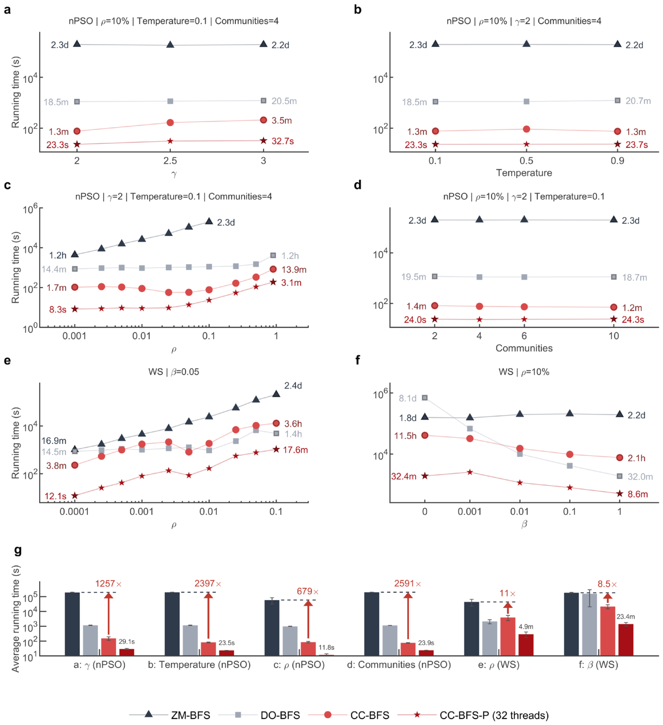

Table 1.
| Time complexity and network suitability of BFS variants for unweighted APSP.
| Algorithm | Description |
General-to-Dense Time Complexity |
Suitable Network Type |
| ZM-BFS | Canonical breadth-first search | O(mn)~O(n3) | Sparse |
| DO-BFS | Direction-optimizing breadth-first search | O(mn)~O(n3) | Dense, small-world |
| CC-BFS | Cannistraci-Chen breadth-first search (this work) | All |
Disclaimer/Publisher’s Note: The statements, opinions and data contained in all publications are solely those of the individual author(s) and contributor(s) and not of MDPI and/or the editor(s). MDPI and/or the editor(s) disclaim responsibility for any injury to people or property resulting from any ideas, methods, instructions or products referred to in the content. |
© 2026 by the authors. Licensee MDPI, Basel, Switzerland. This article is an open access article distributed under the terms and conditions of the Creative Commons Attribution (CC BY) license.
Copyright: This open access article is published under a Creative Commons CC BY 4.0 license, which permit the free download, distribution, and reuse, provided that the author and preprint are cited in any reuse.