

Submitted:
03 November 2026
Posted:
05 November 2026
You are already at the latest version
Abstract
The sustainability literature accounts for training a model, not for keeping a deployed smart-city intrusion detector useful for years. How often the detector is re-trained decides whether it detects anything; within the system boundary modelled, the energy that cadence costs is small beside its detection effect. We replay the five-day CIC-IDS2017 capture (40 flow-count windows, five synthetic districts) under six protocols and twelve re-training policies, charging each re-training its measured CPU time, bytes and ledger transactions, converted under swept assumptions into use-phase energy, carbon, traffic and storage per gateway-year. Never re-trained, the detector scores stream F1 ≤ 0.005; re-training every window brings it to 0.798–0.856 for the edge and federated-averaging learners, and for the edge tree on this replay a label-free feature-drift trigger comes close with 37.5 % of the re-training events; low-rate attacks are largely missed under every policy. At the default assumptions and the replay's thinned traffic (32,000 flows per gateway-day; the share scales with traffic) the estimated upkeep stays below 1 % of a gateway's idle electricity, so the gateway hardware dominates the footprint; raw-traffic export (5.4× edge learning) and ledger storage growth (cut 83 % by Merkle anchoring) are conditional levers. On the ten-day CSE-CIC-IDS2018 capture the cost ordering holds, but the trigger misses attacks that imitate benign traffic and a daily clock fallback recovers only part of the loss.
Keywords:
sustainable smart cities
; urban IoT infrastructure
; operational footprint
; use-phase energy
; carbon footprint
; intrusion detection
; federated learning
; concept drift
; blockchain provenance
; SDG 11
1. Introduction
Sustainable urban development increasingly rests on digital infrastructure: sensing, control and security systems that cities install once and operate for a decade [1,2,3]. The sustainability literature on this infrastructure has concentrated on what it saves—energy in buildings, traffic, water, waste [4,5]—and, more recently, on what the artificial intelligence inside it costs to build [6,7,8,9]. What it costs to keep that intelligence working after deployment has received little attention, although for a security function it is the whole of the operating life: a city does not retrain its intrusion detector for a week and then stop. The United Nations’ 2030 Agenda frames the question through Sustainable Development Goals (SDG) 9 (resilient infrastructure), 11 (sustainable cities) and 13 (climate action) [10]; a municipality that must report on them needs the operating footprint of its security layer, not only its capital footprint. The question this paper answers is a use-phase question in the sense of a sustainability report: once a city has bought its gateways, what does it cost each year, in electricity, carbon, traffic and storage, to keep their intrusion detector working, and which design choices move that cost.
This paper quantifies that operating footprint for one concrete design. In a previous study [11] we built and measured a four-layer security architecture for smart-city Internet-of-Things (IoT) deployments: a lightweight intrusion detector on each district gateway, federated learning across districts so that raw traffic never leaves a district, a permissioned ledger that anchors every model version, and a cloud orchestrator. Two of its measurements set the terms of the present work. First, the energy of detecting is negligible: the deployed depth-8 decision tree spends 0.002 kWh per gateway-year on classification. Second, a detector that is not re-trained stops detecting: trained once on three capture days of CIC-IDS2017 [12], it scored F1 0.0010 and 0.0005 on the next two. Re-training is therefore not an optimisation but the condition of the detector’s usefulness—a finding consistent with time-aware evaluations elsewhere in security machine learning [13,14,15]—and its cost (compute, model traffic across district boundaries, raw-data export, and the provenance records a ledger keeps of every model version) was excluded from that study and, to our knowledge, from the sustainability literature on federated learning [16,17,18], which models training from scratch rather than the steady-state upkeep of a deployed model.
We measure that upkeep. The five-day CIC-IDS2017 capture is replayed as 40 chronological windows; the first two days train the detector and the remaining 24 windows are met one at a time. Twelve re-training policies (never, four clock-driven cadences, two label-free triggers—label-free in the decision to re-train, while every re-training still assumes labelled flows—, the drift trigger with a one-day clock fallback, three standard drift detectors used as triggers and a label-using reference policy) govern six protocols that differ in what crosses the district boundary: edge trees and an edge multilayer perceptron (MLP) that export nothing, federated averaging (FedAvg) [19] and the screened, ledger-anchored poisoning-resilient aggregation (LPRA) of [11] that export weights, and a centralised learner that exports raw flows. Every re-training is charged with its measured CPU time, bytes and ledger transactions, and converted to energy, carbon, traffic and storage per gateway-year and per city-year with explicit, swept assumptions, so that a reader can substitute a measured gateway or a different grid without repeating the experiment. The paper does not propose a new detector: the models are those already deployed in [11], and the quantity of interest is what keeping them alive costs, not how well a better model would detect.
The central finding is that, for a deployed detector under the traffic volumes and assumptions tested here, re-training cadence is a detection decision rather than an energy one: the cadence decides whether the detector still works, and the energy it costs is too small to argue against it, so a city’s sustainability effort is better spent on where traffic is processed, how provenance is recorded and which hardware is bought. The contribution is the accounting and the comparison of policies on a chronological stream, not a new detector or trigger. The contributions are the following. (1) A use-phase accounting method for the security layer of a digital urban system—measured CPU time, bytes and ledger records per re-training, converted with stated and swept assumptions (Equation (1))—applied to a deployed detector and showing that, at the default assumptions, the estimated energy of keeping the detector alive is at most 0.2182 kWh per gateway-year under every policy—at most 0.92% of the gateway’s own idle consumption, and at most 13.8% in the combined worst case—so that the sustainability levers of a municipal deployment are the raw-flow export of centralised learning, the growth of the provenance ledger and the hardware itself, not the re-training cadence. (2) A comparison of re-training policies: daily re-training recovers almost nothing, re-training every window recovers most of the stream F1 (not the low-rate attacks, Section 5.2), and, on the 2017 stream, a label-free feature-drift trigger gives the edge tree a stream F1 within 0.01 of re-training every window (observed paired difference over seeds, interval including zero) with 37.5% of the re-training events (9 of the 24 held-out windows), while an output-based alert-rate trigger never fires. (3) A chronological evaluation of FedAvg and LPRA on this stream, the open item of [11], which shows that, on a stream where a new attack family reaches one district first, the Byzantine screen quarantines about one client update per round and LPRA falls behind FedAvg under frequent small updates. (4) A batched-anchoring design that removes 83–97% of ledger growth without weakening what a district can prove, provided the district keeps its own records and inclusion proofs. (5) A comparison of the trigger with three standard drift detectors—adaptive windowing (ADWIN), Kolmogorov–Smirnov windowing (KSWIN) and the drift detection method (DDM)—and a replay of the whole study on a second, ten-day capture (CSE-CIC-IDS2018) that reproduces the cost ordering, exposes the limit of a label-free feature trigger on attacks that imitate benign traffic, and shows how much of it a clock-driven fallback recovers. Section 5 turns the numbers into procurement, data-governance and reporting guidance for a municipal smart-city programme. Table 1 states what the paper adds to [11], whose architecture, models and measurements it builds on. Readers concerned with the decision rather than the method can read Section 4.1, Section 4.5 and Section 5, which end in a one-table summary of the levers; Section 3 and Section 4.2, Section 4.3, Section 4.4, Section 4.5, Section 4.6, Section 4.7 and Section 4.8 and the supplementary tables S1–S5 carry the evidence behind them.
2. Related Work
2.1. Sustainable Smart Cities and the Footprint of Their Digital Layer
Reviews of sustainable smart cities describe the digital layer as an enabler: IoT sensing and analytics reduce the energy of buildings, grids, mobility and water [2,3,4,5,20], and surveys of IoT-based city management catalogue the platforms that deliver these savings [20,21]. The digital layer’s own footprint is treated, when at all, at the level of the information and communication technology (ICT) sector [22] or of the hardware: embodied carbon now rivals operational carbon for cloud servers and dominates it for compact devices [9]. Security is discussed as a risk to be managed [23,24], rarely as an operating cost to be accounted for; distributed ledgers appear in the sustainability literature as instruments of traceability, for example for agricultural supply chains [25], not as a cost line of the infrastructure that runs them. This paper sits in the gap: it treats the security function of a smart city as infrastructure with an operating footprint of its own, and measures that footprint per gateway-year in the units a sustainability report uses.
2.2. Green AI, Green Edge AI and the Carbon of Learning
Schwartz et al. [8] asked that AI research report efficiency alongside accuracy; the carbon of training in data centres has since been quantified [6,7,26,27] and the tooling for reporting it standardised [27]. At the edge, Mao et al. [28] survey energy-conscious design for data acquisition, training and inference, and note that frugal devices often make edge training cheaper than cloud training in energy, though not in time. For federated learning specifically [29], Qiu et al. [16] gave the first systematic carbon model and found that federated learning can emit up to two orders of magnitude more carbon than centralised training or be comparable when the embedded devices are frugal, and Savazzi et al. [17,18] added communication energy and the parameter server to an end-to-end framework. All of these account for training a model to convergence. The upkeep of a deployed model—short, repeated re-trainings on new data, the traffic each one generates, and the provenance records each one leaves—is a different accounting object, and it is the one a city pays for over the life of a gateway.
2.3. Time-Aware Evaluation and Concept Drift in Security Detectors
Sommer and Paxson [30] set out why learning-based detectors are hard to deploy—the traffic of tomorrow is not the traffic of today—and a decade later Apruzzese et al. [31] found the gap between laboratory and operational performance still open. Pendlebury et al. [13] showed that random splits inflate malware-detector performance and introduced temporally consistent evaluation (TESSERACT); Jordaney et al. [15] proposed conformal evaluation to detect when a classifier’s decisions have drifted; Andresini et al. [14] carried the protocol to network intrusion detection on a revised CIC-IDS2017 and noted that re-training has a cost in processing time and labelling capacity that evaluations should account for. The CIC-IDS2017 capture itself has known defects: Engelen et al. [32] found flow-construction and labelling errors and released a corrected version, and Lanvin et al. [33] showed that correcting them changes measured detection performance; Section 5.2 discusses what that means for the numbers reported here. Cross-dataset studies find the same collapse between captures [34], newer edge-oriented captures such as TON_IoT [35] provide further test beds, and the drift literature supplies the detectors and adaptation strategies [36,37]. This paper takes the test-then-train protocol as given and asks what each re-training decision costs on a stream whose novelty structure is known window by window, and which trigger an operator can compute without labels.
2.4. Edge Gateway Power, Network Transmission Energy and Provenance Ledgers
The power of Raspberry-Pi-class boards has been measured and modelled in the peer-reviewed literature: Kaup et al. [38] fitted a linear power model to the first-generation board, and Bekaroo and Santokhee [39] profiled the board’s draw under its common end-user workloads; for the Pi 4 the manufacturer’s own thermal tests report 2.4–2.9 W idle and 6.7–7.3 W under a four-core synthetic load [40]. The 3 W one-core figure of [11], the 2.7 W idle baseline used here and the 2–10× slowdown sweep bracket these measurements. Aslan et al. [41] estimate the electricity intensity of fixed-line data transmission at 0.06 kWh/GB (2015) and halving about every two years, with mobile access higher; the default and the 0.01–0.30 sweep follow that review. Federated anomaly detection for IoT was introduced by DÏoT [42]; permissioned ledgers [43] with Merkle commitments [44] are the usual provenance layer for federated security; their energy is a matter of consensus design, and permissioned ledgers and proof-of-stake designs such as [45] avoid the proof-of-work cost that dominates public chains, which is why this paper accounts for the ledger in records and bytes rather than in joules; [11] measured anchoring on Hyperledger Fabric 2.5.9 (146 tx/s, 136 ms mean latency, 6,076 B per anchored record, 71% of it certificates). Robust aggregation rules [46,47] protect against poisoning; their behaviour under benign distribution shift, which the chronological protocol exposes, is the subject of Section 4.3.
3. Materials and Methods
3.1. A Chronological Stream of Flow-Count Windows
The study replays the five-day CIC-IDS2017 capture [12] as a stream of 40 windows, eight per capture day. The MachineLearningCVE release carries no timestamp, but its rows are in capture order: every attack family occupies a contiguous row range in exactly the order of the published attack schedule (Tuesday FTP-Patator then SSH-Patator; Wednesday slowloris, Slowhttptest, Hulk, GoldenEye, Heartbleed; Thursday morning Brute Force, XSS, SQL Injection), which the released script tools/verify_row_order.py prints for the released files. Each day is therefore cut into eight consecutive flow-count windows of equal size (on average about one hour of the 09:00–17:00 capture, but the release carries no clock and the windows are not equal in wall-clock time); “daily” in what follows means every eight flow-count windows. The row order reproduces the sequence of the attack blocks, not wall-clock time, so the 2017 replay shows how a detector meets attack families in the order the capture presents them, not temporal drift as a deployment would experience it; that question is put to the timestamp-ordered CSE-CIC-IDS2018 capture in Section 4.8. The stream is built as follows. Each day’s CSV files (MachineLearningCVE release, accessed 30 October 2026) are read in their published order; repeated header rows are dropped; non-numeric, infinite and missing feature values are set to 0; duplicate rows are kept, since they are part of the traffic. A day’s quota of 160,000 flows is split over its files in proportion to their row counts (rounded to the nearest flow), each file is thinned by a seed-controlled draw without replacement, and the drawn rows are put back in file order, so sampling thins the stream without reordering it; each window holds 20,000 flows and the week 800,000. The standardiser and the drift reference of Section 3.4 are fitted on the initial training windows only, and no statistic of a held-out window enters any preprocessing step; the models learn from a held-out window only after it has been scored (Section 3.4). The 77 identifier-free flow features (the CICFlowMeter features without addresses, ports and timestamps) and the binary benign/attack label are those used by [11]. Windows 0–15 (Monday, Tuesday) form the initial training period; the 24 windows of Wednesday–Friday are held out and scored one at a time. They contain every attack family the initial period never saw (Table 2).
3.2. Districts
The K = 5 districts are the synthetic non-IID partition of [11], not a split of real city traffic: benign flows are spread evenly and at random over the five districts, while each attack family has one owner district—families sorted by name are assigned round-robin, family i to district i mod 5—that receives 70% of the family’s flows, the remaining 30% being spread evenly over all five, so that most of an attack arrives in one district. The partition is drawn once per seed for the whole capture, so a district keeps its traffic profile across windows. The 70% dominance is the setting of [11]; how the results move with the degree of imbalance is not tested here (Section 5.2).
3.3. Protocols: Who Learns, and What Crosses the District Boundary
Six protocols are compared (Table 3). The models, optimiser settings and the LPRA screen are the released code of [11]; the standardiser is fitted on the initial training period (pooled statistics, 2 × d numbers, disclosed as before). LPRA is FedAvg with a two-stage screen applied to the K client updates before averaging: stage 1 rejects an update whose distance to the coordinate-wise median of all updates exceeds a robust threshold (the larger of the median plus three median absolute deviations (MAD) and 2.5× the median distance), and stage 2 rejects a survivor whose update direction has cosine below 0.2 with the median direction of the stage-1 survivors; if fewer than a majority pass, the best-aligned majority of the stage-1 survivors is accepted, and the accept/quarantine decision of every district is anchored on the ledger together with the hash of the aggregated model. The MLP(32,16) carries 12,164 bytes of float32 weights, which is what each client uploads and downloads per federated round. The “raw flows” of the centralised protocol are the standardised feature records (77 float32 features and a label, 309 B per flow), not packets; they are exported at each re-training event, so under a trigger policy only the flows up to its last firing leave the district, and the download of the central model to the gateways, where every protocol’s inference is charged, is not counted (12,164 B per re-training, negligible beside the records). The capped tree refits on at most the last 160,000 flows of its district’s history—the city’s daily flow count, hence “1-day history”; at K = 5 a district accumulates about 32,000 flows per day, so the cap is about five district-days of flows at the replay’s thinned rate (“one day” names the city total, and a deployment would set the cap in flows of the gateway’s own traffic); within the five-day replay the cap binds only for the busiest districts in the last windows, the two tree protocols fit nearly the same models (Section 4.1) and differ in their annualised cost (Section 4.4); their CPU-hour differences there (6–32%) are run-to-run timing variation of the same computation on a laptop running four replays at once, not a modelling difference.
3.4. Re-Training Policies: When
At each held-out window the current model scores the window first (that is what is reported); the policy then decides whether to re-train on the flows of the windows since the last re-training (Table 4). This is the prequential (test-then-train) protocol of the stream-learning literature [36,37]: a window is always scored before anything is learned from it. Labels for the flows of the windows since the last re-training are assumed available when the policy decides to re-train, the assumption that every rolling protocol, including that of [11], makes. In a deployment the labels of a window arrive with some delay—from an analyst, a honeypot or a signature engine confirming the alerts—and a label delay of d windows has the same effect as re-training d windows later; the clock-driven policies of Table 4 therefore also read as a label-latency sweep, from one window (every window) to a day (daily). The feature-mean trigger is called the drift trigger in the tables and figures and the feature-drift trigger in the text; the fallback policy, drift trigger + daily fallback in the tables, is the same trigger with a clock fallback of eight windows (Section 4.8).
3.5. What Is Measured, and What Is Assumed
Detection is one of several functions a gateway performs; its packet filtering, whose per-packet processing earlier work on tree-rule firewalls studied at the edge and in the cloud [48,49], draws on the same CPU budget, and the upkeep measured here is to be read against that budget and against the gateway’s idle draw. Measured, per re-training event: process CPU time with the linear-algebra library (BLAS) pinned to one thread; bytes of model traffic and of raw flows exported; ledger transactions generated; and an analytical count of floating-point operations (FLOPs) for the training computation (6 × parameters per sample-epoch for the MLP; n·d·depth·log2 n for the tree) as a hardware-independent cost. Measured, per window: F1, recall, false-positive rate, pooled and per district, and the CPU time of the trigger itself for the detector policies of Section 4.2. Two detection summaries are reported: the mean F1 over the held-out windows (each window equal) and the stream F1 (one confusion matrix over all held-out windows, so volumetric attacks weigh more).
Scope of the account. Included: the CPU time of re-training, inference and the drift detectors; the bytes of model weights and raw flows that cross the district boundary; the ledger records each design writes, as storage and as transmitted bytes. Not included: the electricity of the ledger’s peers and orderers and of the federated aggregation host as always-on nodes (their ordering work is bounded in Section 5.2), the parts of a board’s power that do not scale with CPU time (memory, storage, network interfaces), idle overhead of cloud hosts, the labelling work, and embodied or end-of-life emissions of any device. Carbon is energy multiplied by a stated grid factor, not a measured emission. The gateway’s idle electricity is used only as a reference against which the upkeep is compared, not as the device’s total consumption while it works.
Assumed, in one table (Table 5); the four energy assumptions are each swept one at a time in Section 4.7 and moved together in its combined cases. Energy is measured CPU-seconds scaled by stated board power, exactly as the energy estimate of [11] did, not a wattmeter reading; the relative ordering of policies is stable under the modelled ranges and the stated system boundary because every policy runs the same models on the same windows, and the two hardware constants can be replaced by an on-device measurement without changing anything else in the pipeline. Figure 1 shows how the measured and the assumed quantities combine. All measured inputs are city totals over the n held-out windows of a stream; the annualised energy per gateway is Equation (1), the energy of the whole city is Equation (2), and carbon is Equation (3):
where s = 2,920/n scales the n held-out windows to a year (n = 24 for the 2017 stream, 64 for the 2018 stream), K = 5 is the number of districts, and the two CPU terms, both measured on the x86 host over the test windows, separate the work by where it runs: τgw is the city’s CPU-seconds spent on the gateways—the re-training of the edge and federated protocols, the inference of every protocol and the detector’s own computation where a policy has one—and is scaled by the edge slowdown σ and one-core power Pedge; τcloud is the CPU-seconds spent on the cloud host—the re-training of the centralised protocol, and zero for the others—charged at the host’s own power Px86 with no slowdown. Inet is the network electricity intensity, and Bmod, Braw and Bled are the bytes of model traffic, exported flow records and ledger records (transactions × 6,076 B, the stored record size measured in [11], used here as the proxy for the bytes transmitted when the record is submitted) the city generates over those windows. Every term inside the bracket is a city total; multiplying by s annualises it and dividing by K gives the per-gateway share, so the cloud training and the shared ledger are charged one K-th to each gateway and Equation (2) recovers the city total exactly. Carbon follows from the grid factor fgrid, Equation (3); the idle baseline against which the upkeep is compared is Pidle × 8,760 h per gateway.
Egw = (s / K) · [ (σ · Pedge · τgw + Px86 · τcloud) / (3.6 × 10⁶) + Inet · (Bmod + Braw + Bled) / 109 ]
Ecity = K · Egw
Cgw = fgrid · Egw, Ccity = fgrid · Ecity
Worked example (FedAvg re-trained every window, 2017 stream, mean over seeds), which a reader can check against the measured and scenario tables of Section 4.4 and Section 4.5. Measured, city total over the 24 held-out windows: τtr = 18.5 CPU-s, τinf = 0.3 CPU-s (both on the gateways, so τgw is their sum and τcloud = 0), 14.6 MB of weights and 720 ledger records (4.4 MB). Annualised (× s = 121.67), per city-year: 2,251 training CPU-s; model traffic 1.776 GB, ledger records 0.532 GB, transmitted bytes in all 2.308 GB. Per gateway (÷ K = 5): 450 training CPU-s (0.125 CPU-hours, CPU-h, the figure in the measured table); model traffic 0.355 GB (the measured table’s column), ledger share 0.106 GB, total 0.462 GB, from which the traffic energy is computed. On the edge board (training and inference together, × σ = 5): 2,290 CPU-s, which at 3 W is 0.0019 kWh; the 0.462 GB at 0.06 kWh/GB are 0.0277 kWh. Together 0.0296 kWh per gateway-year (Equation (1)), 0.1480 kWh per city-year (Equation (2)) and 0.0129 kg CO2e per gateway-year at the Thai grid factor (Equation (3)). At the city level the gateway-side terms grow with K and the federated ledger term with K + 1 records per round (Section 4.6).
Energy model and its uncertainty. Equation (1) is the power-times-time model that the carbon-reporting tools of the machine-learning community apply when no meter is attached [26,27] and that PowerPi fitted to the Raspberry Pi as a linear function of CPU utilisation [38]; its inputs here are measured CPU-seconds and bytes, and its two hardware constants and the network intensity are the assumptions. The figures it produces are therefore estimates, and they are reported as such: the one-at-a-time sweep of Section 4.7 bounds the compute term within a factor of 0.4–2 of the default (edge power 2–6 W, slowdown 2–10×) and the traffic term within a factor of 0.17–5 (network intensity 0.01–0.30 kWh/GB), and the combined best and worst cases of Section 4.7 move every energy assumption at once, including the gateway’s duty cycle. What the model cannot capture is the part of a board’s power that does not scale with CPU time—memory, storage and network interfaces—which an on-device measurement would include; that is why the upkeep is always compared with the gateway’s idle draw rather than reported alone.
3.6. Anchoring Granularity
Three designs are compared for the provenance layer. A federated re-training event of R rounds produces R(K + 1) records—in each round K client updates or quarantine decisions and one aggregated model—and an edge re-training event produces K records, one model version per district. Per-record anchoring (the design of [11]) writes each record as its own transaction: R(K + 1) = 30 transactions per federated event at R = 5, K = 5. Per-round anchoring writes one Merkle root over the K + 1 = 6 records of a round (batch b = 6): R = 5 transactions per event. Per-event anchoring writes one root over all R(K + 1) = 30 records of the event (b = 30): one transaction per event; for the edge protocols it batches the K = 5 records of an event. The batch b is the number of records under one root, not a number of rounds. A district can still prove membership of its update or of its quarantine decision with a log2(b)-hash proof against the anchored root [44]; the CPU cost of building roots and proofs and of verifying them is measured with the Merkle code of the emulated ledger of [11].
3.7. Seeds, Hardware and Reproducibility
Five seeds (42–46) control sampling, the district partition and model initialisation; the seed is the unit of analysis. For every protocol–policy pair and seed the stream F1 is computed from one confusion matrix pooled over the held-out windows, and the tables report the mean of the five per-seed values ± the half-width of a 95% t-interval (4 degrees of freedom); these marginal intervals summarise the spread across seeds. Comparisons between policies are made on per-seed paired differences (same seed, same sampling, partition and initialisation), reported as the mean difference with its 95% t-interval and a paired t-test. With five seeds and no adjustment for the number of comparisons, the p-values are exploratory; no comparison is read as showing equivalence, and a small observed difference whose interval includes zero is reported as exactly that. Per-seed values of every detection and cost figure are in Table S2. A stream has 360 replays (6 protocols × 12 policies × 5 seeds), run in three batches as policies were added: 240 for the eight policies of Table 4 that need no drift detector (never, the four clock cadences, the alert-rate and feature-drift triggers and the labelled reference), 90 for ADWIN, KSWIN and DDM, and 30 for the clock fallback; the timings below follow that division. The replays reported here were run on a laptop with an Intel Core i5-11300H (4 cores, 3.10 GHz base, 8 GB of RAM visible to the virtual machine) under Ubuntu 24.04 on the Windows Subsystem for Linux (WSL2; Linux 6.6), Python 3.12.3, NumPy 2.5.4, pandas 3.1.0, scikit-learn 1.9.1, with BLAS pinned to one thread; the 2017 grid took 1 h 02 min with four workers for the first 240 replays and 32 min for the 90 detector replays, the 2018 grid 2 h 36 min with three workers for 330 replays (on an 8 GB machine the 2018 stream needs at most three concurrent replays); the 30 fallback replays added 11 min (2017, four workers) and 20 min (2018, three workers). The 2017 grid run independently on a cloud x86 host (Intel Xeon at 2.10 GHz, Python 3.13.18, NumPy 2.5.3, pandas 3.0.5, scikit-learn 1.9.1) reproduced every detection, traffic and transaction figure of the 2017 replays to the last printed digit (a re-run of the same pipeline on another host, not an independent re-implementation), while its CPU-seconds were about 16% lower (median ratio 1.19); the detection results are therefore independent of the host and of the library versions, and only the CPU-time column is machine-specific. The numbers in the paper are read from results_sustain/paper_facts_sustain.json, produced from the replay files, to support reproduction; the code is a new sustain/ package on top of the released repository of [11] and is cited at a tagged version in the Data Availability Statement.
4. Results
4.1. Without Re-Training the Detector Scores Near Zero, and Daily Re-Training Recovers Little
Under the never policy every protocol scores stream F1 ≤ 0.005 over the 24 held-out windows (Table 6). Daily re-training (after every 8th window) recovers 0.052–0.172: the model fitted at the end of Wednesday has never seen Thursday’s or Friday’s families, so it meets each new day as blind as the never-re-trained model. Detection appears only when re-training keeps pace with the stream: every 2 windows 0.693–0.772, every window 0.798–0.856 for the edge protocols and FedAvg (LPRA is the exception, 0.571, Section 4.3) and 0.933 ± 0.008 for the centralised learner (Figure 2). The mean F1 over windows (Table 7) is lower in every re-training cell, because the equal-weighted mean counts Thursday’s low-rate windows as heavily as the volumetric ones, but it ranks the protocols in the same order. On the 2017 stream the alert-rate trigger never fires and equals never for every protocol, so it is omitted from the tables.
4.2. A Label-Free Drift Trigger and Standard Drift Detectors on the 2017 Stream
The feature-drift trigger fires on the same 9 of the 24 windows in every seed—the four windows of the Wednesday DoS block (16–19) and the five of the Friday PortScan/DDoS block (35–39)—and never on Thursday, whose two web-attack windows carry 1.4–2.5% attacks across the five seeds (1.5–2.2% for the seed of Table 2) and whose infiltration windows at most 0.05%. For the edge tree it scores stream F1 0.852 ± 0.010 against 0.856 ± 0.006 for re-training every window—a paired difference of −0.004 (95% CI [−0.009, +0.001], p = 0.086; a small observed difference whose interval includes zero)—with 1,095 instead of 2,920 re-trainings per year and 0.856 instead of 2.605 CPU-hours per gateway-year (−67%). For FedAvg the comparison is inconclusive (0.779 ± 0.015 against 0.798 ± 0.066; paired difference −0.019, 95% CI [−0.093, +0.055]) at 32,850 instead of 87,600 ledger transactions per year, and for the edge MLP and the centralised learner the trigger costs detection (−0.120 and −0.125, both p < 0.001). The price is paid in false alarms by the MLP-based learners (Table 8): because the trigger fires on attack-dominated windows, continual MLPs re-trained only then drift towards alarming on benign traffic (false-positive rate, FPR, 0.1401 for the edge MLP, 0.0590 for FedAvg, against 0.0203 and 0.0099 under re-training every window); the tree’s FPR rises only from 0.0024 to 0.0040. The small difference is a stream-F1 result: the attack-dense windows dominate that metric and the trigger fires on them. On the equally weighted mean F1 of Table 7 the edge tree scores 0.376 ± 0.007 under the trigger against 0.411 ± 0.015 every window, the gap being the Thursday windows the trigger never re-trains on.
On this stream the output-based alert-rate trigger never fires: a detector that does not see a new attack family raises no alarm whose rate could change. A trigger that watches only the detector’s own output misses exactly the drift that a new family brings.
Standard drift detectors as triggers. The feature-mean trigger above is deliberately simple, and it watches the feature distribution only: it is a proxy for covariate drift, and a change in the relation between features and labels that leaves the feature means inside the initial band is invisible to it, which is what Section 4.8 shows; Table 9 compares it, for four of the protocols (all six in Table S5), with three detectors of the concept-drift literature run as re-training triggers on the same stream, implemented from the original papers and checked against the river library [51]: ADWIN [52] and KSWIN [53], label-free, on a per-flow feature statistic (the mean absolute standardised feature value, averaged over mini-batches of 100 flows, 200 points per window); and DDM [54] on the 0/1 error of the deployed detector on every flow, which needs the labels and therefore sits with the F1-threshold reference policy. Each is reset after a re-training. With the edge tree, ADWIN re-trains 730 times per year for stream F1 0.804, KSWIN 1,728 times for 0.827, and DDM 2,847 times for 0.856, against 1,095 re-trainings and 0.852 for the feature-mean trigger. For the edge tree the feature-mean trigger therefore gives the highest stream F1 of the label-free detectors on this stream: KSWIN re-trains more often for less detection (paired difference to every window −0.029, 95% CI [−0.038, −0.020]), ADWIN re-trains less often but misses part of an onset (its confidence interval is six times wider), and DDM, which sees the labels, re-trains almost every window. For the continual MLP the picture reverses on false alarms: the more frequent label-free trigger avoids the false-alarm rise of Table 8 (FPR 0.0195 under KSWIN against 0.1401 under the feature-mean trigger), so a continual learner wants a trigger that also fires on the return to benign traffic. The detectors themselves cost at most 0.0141 CPU-hours per gateway-year (KSWIN on the full-history tree; Table S5 lists every protocol), negligible next to the re-training they trigger.
4.3. The Byzantine Screen Costs Detection under Frequent Small Updates
LPRA re-trained every window scores 0.571 ± 0.030 against 0.798 ± 0.066 for FedAvg on the same rounds: with one window of new flows per round, the screen quarantines 108 of 600 client updates, about one per round, in almost every re-training. The explanation consistent with the design of the screen is that the update of a district that has just met a new family lies far from the coordinate-wise median of the others and fails the magnitude test; the replay records how many updates were quarantined per round, not which district’s, so this remains a hypothesis to be tested by logging the quarantined district against the family’s arrival. With larger batches the gap closes (every 2 windows 0.693 vs 0.704; drift trigger 0.776 vs 0.779), because the screen then sees several districts move together. This is the chronological evaluation of LPRA that [11] left open; whatever the mechanism, a screen tuned against poisoning [46,47] costs detection when updates are small and frequent. The penalty is a property of the stream as much as of the screen: on the 2018 capture, where each volumetric block reaches every district at once, it does not appear (Section 4.8).
4.4. What Keeping the Detector Alive Costs: Measured Quantities
Table 10 gives, per gateway-year and for the two policies that matter most (every window and the drift trigger), the quantities the replay measures directly: re-trainings, CPU-hours on the x86 host, model traffic, raw flows exported and ledger transactions. They are independent of any accounting assumption. The edge tree spends its cost in refitting (2.605 CPU-hours per gateway-year), the federated protocols in model traffic (0.355 GB per gateway-year up and down) and ledger records (87,600 per year at K = 5), the centralised learner in exporting 3.61 GB of raw flows per gateway-year. The edge MLP is cheapest by two orders of magnitude because a continual pass over a district’s 4,000 new flows costs about 25 ms.
One measured cost is not small: the full-history tree’s refit time grows linearly with the history (fit over all every-window events of the five seeds: 30.2 µs per flow of history, n = 125 fits, the initial fit of each seed included). Integrated over a year of 2,920 re-trainings the city’s history reaches 58 million flows and the cumulative refit cost is 144 CPU-hours per gateway-year on x86—about 721 hours on a 5× slower edge core. This is a lower bound: tree induction is at least linear in the history, and the line is extrapolated far beyond the fitted range (at most 0.8 million flows). The memory grows with it: the district’s own share of the history reaches about 3.6 GB in float32 (18 GB for the city) and has to be held and copied at every refit. Capping the history bounds both: with a full cap in every district (800,000 flows of city history) the fitted line gives 22.0 CPU-s per city-wide re-training event (all five districts), 3.56 CPU-hours per gateway-year on x86 against 144 uncapped, with no loss of detection within the replay (0.856 vs 0.856); the 2.605 CPU-hours of Table 10 is the replay’s own average, taken while the history was still filling.
4.5. An Illustrative Edge-Class Energy and Carbon Scenario
Table 11 converts the measured quantities of Table 10 to energy and carbon for a Raspberry-Pi-class gateway on the Thai grid, with the assumptions of Table 5. This is a scenario, not a measurement: CPU-seconds were measured on an x86 host and scaled by an assumed power and slowdown, as the energy estimate of [11] did, the year is the capture repeated, and every assumption is swept in Section 4.7. Under it, the upkeep of the detector is at most 0.0401 kWh per gateway-year for the edge and federated designs and 0.2182 kWh for the centralised one, which makes raw-flow export 5.4× the most expensive edge design and still 0.92% of the 23.7 kWh the gateway draws idling (2.7 W × 8,760 h). Figure 3 places every protocol and policy on the detection–energy plane and Figure 4 shows where the energy goes. The same estimates without annualisation, which do not depend on the capture repeating, are per re-training event and gateway 0.0137 Wh for the edge tree, 0.0101 Wh for FedAvg and 0.0747 Wh for the centralised learner, or 3.44, 2.53 and 18.68 Wh per million flows the gateway sees.
4.6. Scaling with the Number of Districts and the Anchoring Design
Gateway-side costs are linear in K: a 100-district city re-training every window emits 1.75 kg CO2e per year on the edge tree and 9.5 kg on the centralised design, against 1,034 kg for the same 100 gateways idling (Figure 5a). The ledger is where the federated design writes most: at (K+1) records per round FedAvg writes 87,600 transactions and 532 MB per year at K = 5 and 1.47 million transactions, 9.0 GB, at K = 100; and since every peer keeps a full copy, the storage the city holds in total grows with the number of peers as well. Anchoring one Merkle root per round cuts the ledger to 89 MB (−83%) and one root per re-training event to 18 MB (−97%); a district’s proof of membership is then 96–160 bytes, built in 10–38 µs and verified in 1.9–3.2 µs on the Merkle code of the emulated ledger (Table 12, Figure 5b). The root preserves membership verification on the assumption that the district retains the underlying records and their proofs; it does not guarantee their availability, which remains the district’s own obligation, so the design trades ledger growth for a retention duty. The drift trigger reduces every protocol’s ledger growth by a further 62.5%.
4.7. Sensitivity of the Scenario
Sweeping each assumption of Table 5 one at a time (Table 13, Figure 6) moves the absolute figures by up to 6× (network electricity intensity 0.01–0.30 kWh/GB moves the centralised design from 0.0375 to 1.085 kWh) and changes two orderings. The edge tree and FedAvg, within a factor of 1.4 at the defaults (0.0401 vs 0.0296 kWh), swap places whenever an assumption roughly halves the compute term or raises the traffic term fivefold (edge slowdown 2×, edge power 2 W, network intensity 0.30 kWh/GB); and at the lowest network intensity (0.01 kWh/GB) the centralised learner, whose cost is almost entirely traffic, falls just below the edge tree (0.0375 vs 0.0393 kWh). Under every other assumption the centralised learner is the most energy-intensive protocol, and no assumption touches the measured quantities of Table 10 or the detection results, which do not depend on the scenario at all.
Two quantities the sweep holds fixed deserve the same treatment. The first is traffic volume: the thinned stream gives a gateway about 32,000 flows a day, and every cost in Table 10 grows with the flows the gateway sees. Holding the per-flow cost of Section 4.5 (3.44 Wh per million flows for the edge tree, 18.68 for raw-flow export) constant, the upkeep reaches the gateway’s idle electricity at about 18.9 million flows a day for the edge tree and 3.5 million for raw-flow export; at one million flows a day—a busy district gateway—the edge tree’s upkeep would be 5.3% of the idle draw and raw-flow export 28.8%. The “below 1%” of the default scenario is therefore a statement about the replay’s traffic volume as much as about the designs; the ordering of the designs, and the per-flow figures, do not depend on it. The second is the network intensity: the 0.06 kWh/GB default is the 2015 estimate of Aslan et al. [41], who found it halving about every two years, so a present-day fixed-line value lies below the 0.01 kWh/GB low end of the sweep, at which raw-flow export already costs less than the edge tree (0.0375 vs 0.0393 kWh); whether marginal traffic should carry an average intensity at all is itself disputed, since network electricity is largely fixed [55]. The raw-flow lever of Section 5 is therefore conditional on the intensity: it holds where the network’s electricity is attributed to traffic at more than about 0.01 kWh/GB, and the data-governance argument for keeping flows in the district does not depend on it.
The sweep moves one assumption at a time; Table 14 moves all of them at once. The best case takes the favourable end of every range; the worst case takes the unfavourable end and, in addition, assumes that the gateway carries the capture’s daytime traffic around the clock (24 flow-count windows a day, 8,760 a year) instead of the eight-hour capture day of the default, which is the duty-cycle assumption behind the 2,920 windows per year of Table 5. The idle baseline is held at 2.7 W; at 2.4 W, the low end of the measured range, every share rises by an eighth. Even so the ordering of the three designs is the same in all three combined cases: raw-flow export costs 3.26 kWh per gateway-year in the worst case (13.8% of the idle draw), the edge tree 0.485 kWh (2.1%) and FedAvg 0.438 kWh; in the best case the three designs span 0.0051–0.0375 kWh. Table 14 is a combined case for energy; carbon moves further with the grid factor, from 0.0038 kg CO2e per gateway-year for raw-flow export in the best case (0.10 kg CO2e/kWh) to 2.60 kg in the worst (0.80 kg CO2e/kWh), and 0.388 kg for the edge tree in the worst. The claim the paper makes is therefore the ordering and the order of magnitude—learning at the edge or in the federation at a few per cent of the idle draw at most, raw-flow export 5.4× above it at the defaults and 6.7× in the worst case—not any single figure.
4.8. The Same Study on a Second Capture: CSE-CIC-IDS2018
To check that the findings are not an artefact of one capture week, the whole grid was replayed with the same code on the ten-day CSE-CIC-IDS2018 capture [56]: 80 windows of 20,000 flows (eight per capture day; rounding the per-file quotas leaves a few windows one or two flows short, 1,599,980 flows in all for seed 42) ordered by the Timestamp column of the release, 76 identifier-free features (the release lacks one of the 2017 columns), the first two capture days as the initial training period and 64 held-out windows (Table 15). The schedule differs from 2017 in two ways that matter here: each attack family occupies its own day or two, and the initial period already contains brute-force and DoS attacks.
Because the initial period already contains attacks, the deploy-and-forget detector is not blind on this stream: it scores stream F1 0.257 (edge tree) to 0.454 (MLP-based learners) on the held-out windows (Table 16), almost all of it on the DoS Hulk and SlowHTTPTest block of 16 February, whose flows resemble the DoS flows it was trained on. Re-training still decides the outcome: every window restores 0.773–0.820 for the edge and FedAvg learners and 0.801 centrally (here the capped edge tree, 0.820, is the best detector of the six), while daily re-training (0.348–0.464) adds little over never and for the edge MLP, FedAvg and LPRA is worse (FedAvg 0.418 against 0.454): a model refitted on one day’s flows forgets the families of the days before. The LPRA penalty of Section 4.3 does not recur: LPRA re-trained every window scores 0.780 against 0.773 for FedAvg although the screen quarantined 310 of 1,600 client updates, because on this stream the volumetric blocks reach every district at once and the quarantined update is rarely the only informative one.
The feature-mean drift trigger shows its limit here (Figure 7). It fires on 17–18 of the 64 held-out windows, the count varying with the seed (785 re-trainings a year once annualised, 26.9% of every window)—every one of them inside one of the two volumetric blocks (DoS on 16 February, DDoS HOIC on 21 February) or on the window just after it—and scores 0.694 for the edge tree and 0.709 centrally against 0.820 and 0.801 every window (paired differences −0.126, 95% CI [−0.155, −0.097], and −0.092, [−0.117, −0.067]). The LOIC-HTTP flood at a third of the traffic, the web attacks, the infiltration of 28 February–1 March and the botnet of 2 March leave the feature means inside the band of the initial period, so the trigger stays silent and the detector scores close to zero on those days, where re-training every window recovers part of the botnet (F1 0.99 on its last windows) and a little of the infiltration. The alert-rate trigger, silent on 2017, fires a few times here (2–5 of the 64 windows for the edge trees, inside or at the end of the 16 February DoS block; the MLP-based learners fire 3–11 times and once or twice on the 28 February infiltration day) but adds almost nothing (0.275 for the edge tree against 0.257 never). ADWIN is blind in the same way as the feature-mean trigger (6 events, 0.519); KSWIN, which reacts to any change of the statistic’s distribution rather than to its distance from a reference, re-trains on 36 windows for 0.670, and DDM, which sees the labels, on 60 for 0.814. A feature-distribution trigger sees what changes the shape of the traffic and nothing else; attacks that imitate benign flows change neither the alarms nor the feature means.
A clock-driven fallback, tested. The remedy that follows is to re-train when the trigger fires or, failing that, once a capture day (eight flow-count windows) has passed. Run as a twelfth policy on both streams, it recovers part of the loss on this stream and not all of it: the edge tree rises from 0.694 to 0.740 (paired difference to every window −0.080, 95% CI [−0.117, −0.043]) at 1,004 re-trainings per year, and the MLP-based and centralised learners gain less (Table 17). A one-day clock is too slow for this capture’s attacks for the same reason that daily re-training is (0.374 for the edge tree, Table 16): what the stream needs is re-training every one or two windows (0.749 at every second window, 1,460 re-trainings per year) or, for the edge tree, a label-using trigger (DDM, 0.814 on 60 of 64 windows). On the 2017 stream the fallback costs the edge tree nothing in detection (0.851, paired difference to every window −0.005, 95% CI [−0.011, +0.001]) and reduces the edge MLP’s false-alarm drift (FPR 0.1401 → 0.0679, still above the 0.0203 of re-training every window; F1 0.710 → 0.770), while for the continual MLP and the centralised learner it remains below re-training every window (−0.059 and −0.089). The fallback interval is therefore a parameter to be set by the attack mix a city expects, not a constant.
The cost side reproduces the 2017 ordering (Table 18). On this ten-day stream the one-day history cap binds from the sixth day on, and its effect is visible inside the replay: the capped edge tree spends 1.887 CPU-hours per gateway-year re-training every window against 2.841 for the full-history tree, for similar detection, and 0.268 under the drift trigger; uncapped, the refit would grow to 123 CPU-hours per gateway-year; the federated protocols spend their cost in model traffic and ledger records and the centralised learner in exporting 3.56 GB of raw flows (1.35 GB under the drift trigger, whose last firing at the end of the 21 February block leaves the later flows unexported—a property of the finite replay, not of the policy). In the edge-class scenario the upkeep is at most 0.0437 kWh per gateway-year for the edge and federated designs and 0.2149 kWh for raw-flow export, 0.91% of the gateway’s idle draw: the levers of Section 5.1 and the size of each effect carry over unchanged.
What the second capture settles and what it does not: the cost ordering of the designs (edge and federated below raw-flow export), the per-event and per-flow costs, the growth of the full-history refit and the detection collapse without re-training hold on both streams; the near-zero F1 of the never-re-trained detector, the parity of the feature-drift trigger with re-training every window, the LPRA penalty and the adequacy of a one-day fallback hold only on the 2017 stream and depend on the order and the mix of attacks in a capture.
5. Discussion
5.1. What the Numbers Mean for a Municipality
Under the modelled assumptions, re-training cadence changes the upkeep less than any other design choice examined here; it is a security requirement with a small energy cost. At the default assumptions the estimated upkeep of the detector is below 1% of the gateway’s own idle electricity under every protocol and policy (at most 13.8% for raw-flow export and 2.1% for edge learning in the combined worst case of Table 14), and the measured quantities behind it (Table 10) are small in absolute terms: about 2.6 CPU-hours for the edge tree, 0.36 GB of model traffic for FedAvg (ledger records excluded) or 3.6 GB of raw flows for the centralised learner, per gateway-year. A municipality that defers re-training to save energy saves at most 0.0401 kWh per gateway-year (0.0437 on the 2018 stream), and only by never re-training, and loses the detector (stream F1 from 0.856 to 0.137 at daily cadence and 0.005 never). Under the modelled assumptions, labelling capacity and operations weigh more on that decision than energy does. Table 19 collects the levers that do move the footprint, with the size of each effect and the part of a municipal programme that controls it.
The detection–energy trade-off on the 2017 stream is Figure 3: every step up the detection–energy frontier (as labelled in Figure 3) below the centralised learner costs less than 0.02 kWh per gateway-year (on the 2018 stream the largest such step is 0.026 kWh), and the one step with a material energy cost, exporting raw flows to a cloud learner (about 0.18 kWh more for F1 0.856 → 0.933, both re-trained every window), is also the one that moves raw network-flow records out of the district. Flow records describe who communicated with whom and when, and in a deployment they would carry the addresses removed from the research features; whether they are personal data under the Thai Personal Data Protection Act [57] or the GDPR depends on what is exported and is a legal question this paper does not settle, but keeping them in the district avoids it. Provenance storage grows with (K+1) records per round and with K itself; per-round Merkle anchoring removes 83% of it at the cost of a 96-byte proof per district. The hardware dominates: 100 idling gateways emit 1,034 kg CO2e per year against 1.75 kg for keeping their detectors alive, so the gateway’s sleep states, power-supply efficiency and embodied carbon weigh several hundred times more than the learning (about 590× at the default assumptions).
The cost the energy account does not contain is labelling, and here the replay makes a strong assumption that should be named: every flow used for re-training carries its correct label when the policy decides to re-train (a perfect, immediate-label assumption). A supervised detector needs a label for every flow it trains on, benign or not, so the flows that enter training and the flows that must be labelled are the same set—58.4 million per city-year at this sampling rate, about 32,000 per gateway-day under any policy that keeps re-training—and the policy changes only how soon the labels must be ready (Section 3.4) and how much compute follows. In practice such labels come from a signature engine, a honeypot, an analyst’s confirmation of alerts, or a rule that flows nobody flagged are benign; the last makes the analyst’s workload the alerts rather than every flow, but it turns every missed attack into a benign training label, so the cheaper labelling pipeline feeds the detector’s own false negatives back into training. Neither the cost of a labelling pipeline nor the effect of its errors is measured here. A municipality should cost the labelling pipeline before the energy: under the modelled assumptions the energy will not change the decision, the labelling may.
Trigger on traffic, not on alarms—and keep a clock. On the 2017 stream a feature-distribution trigger that any gateway can compute without labels gives the edge tree a stream F1 within 0.01 of re-training every window with 37.5% of the re-training events (9 of the 24 held-out windows); an alarm-rate trigger is blind by construction. The trigger’s cost there is a higher false-alarm rate for continual MLPs; the depth-8 tree, re-fitted on a one-day history, is both the most accurate edge learner and the one least affected. The 2018 stream shows the limit: the trigger is silent on infiltration and botnet traffic that imitates benign flows. Pairing it with a one-day clock fallback, tested on both streams (Section 4.8), costs the edge tree and FedAvg nothing on the 2017 stream (for the continual MLP and the centralised learner the paired differences are −0.059 and −0.089, Table 17) and recovers about a third of the edge tree’s loss on the 2018 stream; there, closing the gap needed re-training every one or two windows or a label-using trigger. The fallback interval should be set by the attack mix a city expects, and the evidence for any interval comes from these two captures only.
The screened aggregation needs a larger batch. LPRA’s protection against poisoning becomes a liability when updates are small and frequent: it quarantines the district that has just seen the new attack. Re-training on at least two windows, or on a drift trigger, removes the penalty, and on the 2018 stream, where attacks reach every district at once, it does not arise. A screen that distinguishes a coherent shift of several districts from a single outlier is an open design question.
5.2. Limitations and Threats to Validity
Construct validity—no on-device measurement. The energy and carbon figures of Section 4.5 are a scenario: CPU-seconds were measured on an x86 host and scaled to an edge board with a stated power and slowdown, as the energy estimate of [11] did; the sweep (2–10×, 2–6 W) brackets published Raspberry Pi 4 measurements [40], and the relative ordering of policies is stable under the modelled ranges because every policy runs the same models on the same windows. The two constants enter Equation (1) linearly and multiply every policy alike, so they scale the absolute figures but cannot reverse the central finding within the swept range: with both, and the duty cycle, at their unfavourable ends the upkeep is still at most 13.8% of the gateway’s idle draw for raw-flow export and 2.1% for edge learning (Table 14), while not re-training still costs the detector. An on-device measurement on a Raspberry-Pi-class gateway is the next step; the replay already records the CPU-seconds of every re-training event, so it needs only the board’s measured power and run time per refit, and nothing else in the pipeline changes.
External validity—two captures, each scaled to a year. The annual figures assume the capture’s traffic and attack mix repeats; they are a scenario for comparing policies, not a forecast, and the 2018 replay (Section 4.8) shows how much the absolute detection figures depend on the schedule of a capture while the cost ordering does not. The flow-count windows average about an hour of capture but are not clocked, and the eight windows a day of the default annualisation assume the capture’s traffic for eight hours and nothing comparable for the other sixteen; the worst case of Table 14 removes that assumption. The five districts are a synthetic partition with a fixed 70% dominance; real districts may be more or less imbalanced, and how the federated results move with the imbalance is not tested. Internal validity—labels are assumed correct and available at re-training time (the perfect, immediate-label assumption of Section 5.1), the assumption of every rolling protocol including that of [11]; the labelling cost is the dominant operational cost the paper does not measure. Network energy uses a fixed-line intensity; a cellular backhaul raises the traffic terms by up to 5× (swept). The ledger energy is accounted as storage and transaction count, not as peer and orderer electricity; a bound follows from the measured Fabric throughput of [11] (146 tx/s): the 87,600 transactions of FedAvg re-trained every window occupy the ordering service for about 600 s per year, which at an assumed 100 W for the whole peer network is 0.017 kWh per city-year—about an eighth of the energy of FedAvg’s model traffic and far below raw-flow export. The peers and orderers themselves, like the aggregation host of the federated protocols, are always-on infrastructure outside the system boundary of Section 3.5: a single node drawing 10 W uses about 88 kWh a year, more than the detection upkeep of the whole city under any protocol, so for a municipality the provenance lever is the number and the idle power of the ledger nodes before it is the ledger’s growth. Thursday’s low-rate attacks (web attacks at 1.4–2.5% of their two windows across seeds, infiltration at most 0.05%) are largely missed: only re-training every window catches part of the second web-attack window after learning from the first (recall 0.18–0.91 across protocols), and infiltration stays below 0.35 recall (mean over seeds; single windows hold only a handful of infiltration flows) under every protocol and policy; the stream F1 is carried by the volumetric families, as in [11]. The capture also carries the labelling and flow-construction defects documented by Engelen et al. [32] and Lanvin et al. [33]; they move absolute detection figures, but every policy and protocol here is scored on the same labels of the same windows, so the ordering of policies and the cost of each re-training event, which depend on flow counts rather than on labels, are not affected in the same way.
5.3. Implications for a Municipal Smart-City Programme
- Procurement: require a re-training history cap in flows, set from the gateway’s throughput and memory budget (160,000 flows, one capture day of city traffic, is the value tested here, not a standard), and a drift trigger with a clock fallback calibrated and evaluated on the city’s own traffic and threat model against pre-specified recall, false-positive and re-training-cost criteria (the one-day fallback tested here is a scenario, not a validated setting); specify gateway idle power, which dominates the footprint.
- Data governance: keep raw flows in the district; the federated design’s privacy benefit costs no more energy than the edge tree and about seven times less than central export.
- Provenance: anchor one Merkle root per round (or per re-training event) and keep proofs with the parties; the ledger then grows at 18–89 MB per year for five districts.
- Reporting: on both streams the detection upkeep can be stated in a sustainability report as below 0.1 kg CO2e per gateway-year at the TGO grid factor (0.0954 kg for raw-flow export on the 2017 stream), and below 0.02 kg when raw flows stay in the district (0.0175 kg).
These are requirements to be tested against a city’s own traffic and threat model before they become defaults: the trigger’s cost in false alarms for continual learners (Table 8) and its silence on attacks that imitate benign traffic (Section 4.8) are the two acceptance tests, and a tender should state the recall and false-positive rates it will accept. With that proviso, the five lines a municipality can write into the requirement are: (i) the gateway learns on its own traffic or exchanges model weights only; raw flows do not leave the district; (ii) the detector is re-trained on a feature-drift trigger with a clock-driven fallback, both calibrated on the city’s traffic and threat model against stated recall and false-positive criteria (one day sufficed on one capture tested here and not on the other), on a history capped at a number of flows set from the gateway’s throughput and memory (160,000 here); (iii) model versions and aggregation decisions are anchored on the ledger one Merkle root per round, with proofs kept by the districts; (iv) the gateway’s idle power and sleep states are specified and measured at acceptance, because they dominate the footprint; (v) the detection upkeep is reported per gateway-year with the accounting of Table 5 and Equation (1), so that it can be audited and compared across tenders.
6. Conclusions
For a city that runs intrusion detection at the edge, re-training cadence is a detection decision, not an energy one, under the traffic volumes and assumptions tested here. On a 40-window chronological replay of CIC-IDS2017, a smart-city intrusion detector that is not re-trained scores near zero (stream F1 ≤ 0.005; a floor set partly by the stream, whose initial period holds only two attack families) and one re-trained daily scores little better (0.052–0.172); re-training every window restores 0.798–0.856 for the edge and FedAvg learners (LPRA excepted) and 0.933 centrally. In the edge-class scenario, annualised from this capture week, keeping the detector alive is estimated to cost 0.0014–0.0401 kWh per gateway-year for the edge and federated designs and 0.2182 kWh for the centralised one—under 1% of the gateway’s idle draw at the default assumptions, and at most 13.8% (raw-flow export) or 2.1% (edge learning) when every energy assumption, the duty cycle included, is taken at its unfavourable end—so under the modelled assumptions the levers are the raw-flow export, the provenance ledger’s storage growth and the hardware rather than the re-training cadence. On this stream a feature-drift trigger that needs no labels to decide (the re-training it starts still does) gives the edge tree a stream F1 within 0.01 of re-training every window with 37.5% of the events (9 of 24 held-out windows), and an alarm-rate trigger never fires. On it the Byzantine screen of the previous architecture also quarantines about one client update per round under frequent small updates and falls behind FedAvg, and a full-history refit grows to 144 CPU-hours per gateway-year, and to a history of 3.6 GB per district, unless the history is capped. Per-round Merkle anchoring removes 83% of the ledger growth without weakening what a district can prove, as long as the district keeps its own records and proofs. On the ten-day CSE-CIC-IDS2018 capture the cost ordering and the levers carry over unchanged, while the label-free feature trigger is silent on infiltration and botnet traffic that imitates benign flows; a one-day clock fallback recovers only part of that loss, so the fallback interval has to be set by the attack mix a deployment expects. Three kinds of statement should be kept apart when these results are used. Measured in the replay: CPU-seconds, bytes and ledger transactions per re-training event, and the detection metrics of every window. Estimated from stated assumptions: the kWh, kg CO2e and per-gateway-year figures, which hold within the modelled traffic volume, duty cycle, network intensity and system boundary, and exclude labelling effort, always-on ledger and aggregation infrastructure, the non-CPU power of the gateway and embodied impacts. Proposed for a city: the levers and the tender lines of Section 5, which are starting points to be tested against the city’s own traffic, hardware, labelling capacity and threat model. The code, configuration and replay files are released to support reproduction, and the two hardware constants can be replaced by on-device measurements without changing the pipeline.
Supplementary Materials
The following supporting information can be downloaded at the website of this paper posted on Preprints.org. The following supporting information can be downloaded at the article page: Table S1 the full window schedules (40 and 80 windows; flows, attack share, families present and first seen per window); Table S2 the detection–cost grid for all 72 protocol–policy pairs with per-seed values; Table S3 per-window F1, recall and FPR for every replay; Table S4 the scaling table (K = 5–100); Table S5 every protocol under every re-training trigger, each for both streams; the replay files replay_<protocol>_<policy>_s<seed>.json with every per-window metric and per-event cost record.
Author Contributions
Conceptualization, T.C. and S.P.; methodology, T.C. and S.P.; formal analysis, T.C. and S.P.; software, T.C. and S.P.; validation, T.C. and S.P.; writing—original draft preparation, T.C. and S.P.; writing—review and editing, T.C. and S.P.; visualization, T.C. and S.P.; supervision, T.C. and S.P.; project administration, T.C. and S.P. All authors have read and agreed to the published version of the manuscript.
Funding
This research project was financially supported by Mahasarakham University.
Institutional Review Board Statement
Not applicable.
Informed Consent Statement
Not applicable.
Data Availability Statement
The datasets analysed in this study are publicly available: CIC-IDS2017, MachineLearningCVE release (unb.ca/cic/datasets, accessed on 30 October 2026) and CSE-CIC-IDS2018, the Processed Traffic Data for ML Algorithms release on AWS Open Data (accessed on 30 October 2026). The complete experimental code (the sustain/ package on top of the released repository of [11]), the configuration used for every experiment, the replay files behind every table and figure, and the scripts that regenerate this manuscript’s numbers are openly available at https://github.com/thawatchai2799/SecurityArchitectureSmartCityIoT (accessed on 30 October 2026). The results reported here correspond to the tagged release v3.0-sustainability, and README_SUSTAIN.md in the repository maps every table and figure to the script and result file that produce it.
Acknowledgments
During the preparation of this work the authors used Claude (Anthropic; models Claude Fable 5.1 and Claude Opus 5.5) to assist with software implementation, numerical computation, literature search, and drafting of the manuscript text. The research questions, all modelling decisions, the empirical data collection, verification of the results against the primary literature, and the final scientific judgements are the authors’ own. The authors reviewed and edited all content produced with these tools and take full responsibility for the content of the publication.
Conflicts of Interest
The authors declare no conflicts of interest.
Abbreviations
The following abbreviations are used in this manuscript:
| Abbreviation | Meaning | Abbreviation | Meaning |
| ADWIN | adaptive windowing drift detector | IoT | Internet of Things |
| BLAS | Basic Linear Algebra Subprograms | KSWIN | Kolmogorov–Smirnov windowing drift detector |
| CI | confidence interval | LPRA | ledger-anchored, poisoning-resilient aggregation |
| CPU-h | CPU-hours | MAD | median absolute deviation |
| CO2e | carbon-dioxide equivalent | tx | ledger transaction(s) |
| CSV | comma-separated values | gw-yr | gateway-year |
| RAM | random-access memory | ||
| DDM | drift detection method | MLP | multilayer perceptron |
| DDoS | distributed denial of service | SD | standard deviation |
| DoS | denial of service | TGO | Thailand Greenhouse Gas Management Organization |
| FedAvg | federated averaging | WSL2 | Windows Subsystem for Linux, version 2 |
| FPR | false-positive rate | XSS | cross-site scripting |
| GDPR | General Data Protection Regulation (EU) | SDG | Sustainable Development Goal |
| ICT | information and communication technology | FLOPs | floating-point operations |
References
- Bibri, S.E.; Krogstie, J. Smart sustainable cities of the future: An extensive interdisciplinary literature review. Sustain. Cities Soc. 2017, 31, 183–212. [Google Scholar] [CrossRef]
- Bibri, S.E.; Alexandre, A.; Sharifi, A.; Krogstie, J. Environmentally sustainable smart cities and their converging AI, IoT, and big data technologies and solutions: An integrated approach to an extensive literature review. Energy Inform. 2023, 6, 9. [Google Scholar] [CrossRef]
- Silva, B.N.; Khan, M.; Han, K. Towards sustainable smart cities: A review of trends, architectures, components, and open challenges in smart cities. Sustain. Cities Soc. 2018, 38, 697–713. [Google Scholar] [CrossRef]
- Al-Obaidi, K.M.; Hossain, M.; Alduais, N.A.M.; Al-Duais, H.S.; Omrany, H.; Ghaffarianhoseini, A. A review of using IoT for energy efficient buildings and cities: A built environment perspective. Energies 2022, 15, 5991. [Google Scholar] [CrossRef]
- Mishra, P.; Singh, G. Energy management systems in sustainable smart cities based on the Internet of Energy: A technical review. Energies 2023, 16, 6903. [Google Scholar] [CrossRef]
- Strubell, E.; Ganesh, A.; McCallum, A. Energy and policy considerations for deep learning in NLP. In Proceedings of the 57th Annual Meeting of the Association for Computational Linguistics (ACL), Florence, Italy, 28 July–2 August 2019; pp. 3645–3650. [Google Scholar]
- Patterson, D.; Gonzalez, J.; Hölzle, U.; Le, Q.; Liang, C.; Munguia, L.-M.; Rothchild, D.; So, D.R.; Texier, M.; Dean, J. The carbon footprint of machine learning training will plateau, then shrink. Computer 2022, 55, 18–28. [Google Scholar] [CrossRef]
- Schwartz, R.; Dodge, J.; Smith, N.A.; Etzioni, O. Green AI. Commun. ACM 2020, 63, 54–63. [Google Scholar] [CrossRef]
- Gupta, U.; Kim, Y.G.; Lee, S.; Tse, J.; Lee, H.-H.S.; Wei, G.-Y.; Brooks, D.; Wu, C.-J. Chasing carbon: The elusive environmental footprint of computing. In Proceedings of the IEEE International Symposium on High-Performance Computer Architecture (HPCA), Seoul, Korea, 27 February–3 March 2021; pp. 854–867. [Google Scholar]
- United Nations. Transforming Our World: The 2030 Agenda for Sustainable Development; A/RES/70/1; United Nations: New York, NY, USA, 2015. [Google Scholar]
- Chomsiri, T.; Phunsa, S. A multi-layer security architecture for smart-city IoT with measured limits: Edge intrusion detection, screened federated learning and ledger-anchored model provenance. Smart Cities 2026, 9, 171. [Google Scholar] [CrossRef]
- Sharafaldin, I.; Lashkari, A.H.; Ghorbani, A.A. Toward generating a new intrusion detection dataset and intrusion traffic characterization. In Proceedings of the 4th International Conference on Information Systems Security and Privacy (ICISSP), Funchal, Portugal, 22–24 January 2018; pp. 108–116. [Google Scholar]
- Pendlebury, F.; Pierazzi, F.; Jordaney, R.; Kinder, J.; Cavallaro, L. TESSERACT: Eliminating experimental bias in malware classification across space and time. In Proceedings of the 28th USENIX Security Symposium, Santa Clara, CA, USA, 14–16 August 2019; pp. 729–746. [Google Scholar]
- Andresini, G.; Pendlebury, F.; Pierazzi, F.; Loglisci, C.; Appice, A.; Cavallaro, L. INSOMNIA: Towards concept-drift robustness in network intrusion detection. In Proceedings of the 14th ACM Workshop on Artificial Intelligence and Security (AISec), Virtual, 15 November 2021; pp. 111–122. [Google Scholar]
- Jordaney, R.; Sharad, K.; Dash, S.K.; Wang, Z.; Papini, D.; Nouretdinov, I.; Cavallaro, L. Transcend: Detecting concept drift in malware classification models. In Proceedings of the 26th USENIX Security Symposium, Vancouver, BC, Canada, 16–18 August 2017; pp. 625–642. [Google Scholar]
- Qiu, X.; Parcollet, T.; Fernandez-Marques, J.; Gusmao, P.P.B.; Gao, Y.; Beutel, D.J.; Topal, T.; Mathur, A.; Lane, N.D. A first look into the carbon footprint of federated learning. J. Mach. Learn. Res. 2023, 24, 1–23. [Google Scholar]
- Savazzi, S.; Kianoush, S.; Rampa, V.; Bennis, M. A framework for energy and carbon footprint analysis of distributed and federated edge learning. In Proceedings of the IEEE 32nd Annual International Symposium on Personal, Indoor and Mobile Radio Communications (PIMRC), Helsinki, Finland, 13–16 September 2021; pp. 1564–1569. [Google Scholar]
- Savazzi, S.; Rampa, V.; Kianoush, S.; Bennis, M. An energy and carbon footprint analysis of distributed and federated learning. IEEE Trans. Green Commun. Netw. 2023, 7, 248–264. [Google Scholar] [CrossRef]
- McMahan, B.; Moore, E.; Ramage, D.; Hampson, S.; Agüera y Arcas, B. Communication-efficient learning of deep networks from decentralized data. In Proceedings of the 20th International Conference on Artificial Intelligence and Statistics (AISTATS), Fort Lauderdale, FL, USA, 20–22 April 2017; pp. 1273–1282. [Google Scholar]
- Zaman, M.; Puryear, N.; Abdelwahed, S.; Zohrabi, N. A review of IoT-based smart city development and management. Smart Cities 2024, 7, 1462–1501. [Google Scholar] [CrossRef]
- Syed, A.S.; Sierra-Sosa, D.; Kumar, A.; Elmaghraby, A. IoT in smart cities: A survey of technologies, practices and challenges. Smart Cities 2021, 4, 429–475. [Google Scholar] [CrossRef]
- Malmodin, J.; Lundén, D. The energy and carbon footprint of the global ICT and E&M sectors 2010–2015. Sustainability 2018, 10, 3027. [Google Scholar] [CrossRef]
- Ismagilova, E.; Hughes, L.; Rana, N.P.; Dwivedi, Y.K. Security, privacy and risks within smart cities: Literature review and development of a smart city interaction framework. Inf. Syst. Front. 2022, 24, 393–414. [Google Scholar] [CrossRef]
- Sharma, R.; Arya, R. Security threats and measures in the Internet of Things for smart city infrastructure: A state of art. Trans. Emerg. Telecommun. Technol. 2023, 34, e4571. [Google Scholar] [CrossRef]
- Phunsa, S.; Noiumkar, P.; Chomsiri, T. Survey and analysis of NFT and blockchain technologies for developing agricultural product trading systems. In Proceedings of the 20th International Joint Conference on Computer Science and Software Engineering (JCSSE), Phitsanulok, Thailand, 28 June–1 July 2023; pp. 145–149. [Google Scholar]
- Lacoste, A.; Luccioni, A.; Schmidt, V.; Dandres, T. Quantifying the carbon emissions of machine learning. arXiv 2019, arXiv:1910.09700. [Google Scholar]
- Henderson, P.; Hu, J.; Romoff, J.; Brunskill, E.; Jurafsky, D.; Pineau, J. Towards the systematic reporting of the energy and carbon footprints of machine learning. J. Mach. Learn. Res. 2020, 21, 1–43. [Google Scholar]
- Mao, Y.; Yu, X.; Huang, K.; Zhang, Y.-J.A.; Zhang, J. Green edge AI: A contemporary survey. Proc. IEEE 2024, 112, 880–911. [Google Scholar] [CrossRef]
- Kairouz, P.; McMahan, H.B.; Avent, B.; et al. Advances and open problems in federated learning. Found. Trends Mach. Learn. 2021, 14, 1–210. [Google Scholar] [CrossRef]
- Sommer, R.; Paxson, V. Outside the closed world: On using machine learning for network intrusion detection. In Proceedings of the IEEE Symposium on Security and Privacy, Oakland, CA, USA, 16–19 May 2010; pp. 305–316. [Google Scholar]
- Apruzzese, G.; Laskov, P.; Montes de Oca, E.; Mallouli, W.; Burdalo Rapa, L.; Grammatopoulos, A.V.; Di Franco, F. The role of machine learning in cybersecurity. Digit. Threat. Res. Pract. 2023, 4, 8. [Google Scholar] [CrossRef]
- Engelen, G.; Rimmer, V.; Joosen, W. Troubleshooting an intrusion detection dataset: The CICIDS2017 case study. In Proceedings of the IEEE Security and Privacy Workshops (SPW), San Francisco, CA, USA, 27 May 2021; pp. 7–12. [Google Scholar]
- Lanvin, M.; Gimenez, P.-F.; Han, Y.; Majorczyk, F.; Mé, L.; Totel, E. Errors in the CICIDS2017 dataset and the significant differences in detection performances it makes. In Risks and Security of Internet and Systems (CRiSIS 2022); LNCS 13857; Springer: Cham, Switzerland, 2023; pp. 18–33. [Google Scholar]
- Cantone, M.; Marrocco, C.; Bria, A. Machine learning in network intrusion detection: A cross-dataset generalization study. IEEE Access 2024, 12, 144489–144508. [Google Scholar] [CrossRef]
- Moustafa, N. A new distributed architecture for evaluating AI-based security systems at the edge: Network TON_IoT datasets. Sustain. Cities Soc. 2021, 72, 102994. [Google Scholar] [CrossRef]
- Gama, J.; Žliobaitė, I.; Bifet, A.; Pechenizkiy, M.; Bouchachia, A. A survey on concept drift adaptation. ACM Comput. Surv. 2014, 46, 44. [Google Scholar] [CrossRef]
- Lu, J.; Liu, A.; Dong, F.; Gu, F.; Gama, J.; Zhang, G. Learning under concept drift: A review. IEEE Trans. Knowl. Data Eng. 2019, 31, 2346–2363. [Google Scholar] [CrossRef]
- Kaup, F.; Gottschling, P.; Hausheer, D. PowerPi: Measuring and modeling the power consumption of the Raspberry Pi. In Proceedings of the 39th IEEE Conference on Local Computer Networks (LCN), Edmonton, AB, Canada, 8–11 September 2014; pp. 236–243. [Google Scholar]
- Bekaroo, G.; Santokhee, A. Power consumption of the Raspberry Pi: A comparative analysis. In Proceedings of the IEEE International Conference on Emerging Technologies and Innovative Business Practices for the Transformation of Societies (EmergiTech), Balaclava, Mauritius, 3–6 August 2016; pp. 361–366. [Google Scholar]
- Halfacree, G. Thermal testing Raspberry Pi 4. Raspberry Pi Foundation blog, 2019. Available online: https://www.raspberrypi.com/news/thermal-testing-raspberry-pi-4/ (accessed on 30 October 2026).
- Aslan, J.; Mayers, K.; Koomey, J.G.; France, C. Electricity intensity of Internet data transmission: Untangling the estimates. J. Ind. Ecol. 2018, 22, 785–798. [Google Scholar] [CrossRef]
- Nguyen, T.D.; Marchal, S.; Miettinen, M.; Fereidooni, H.; Asokan, N.; Sadeghi, A.-R. DÏoT: A federated self-learning anomaly detection system for IoT. In Proceedings of the 39th IEEE International Conference on Distributed Computing Systems (ICDCS), Dallas, TX, USA, 7–10 July 2019; pp. 756–767. [Google Scholar]
- Androulaki, E.; Barger, A.; Bortnikov, V.; et al. Hyperledger Fabric: A distributed operating system for permissioned blockchains. In Proceedings of the 13th EuroSys Conference, Porto, Portugal, 23–26 April 2018; pp. 1–15. [Google Scholar]
- Merkle, R.C. A digital signature based on a conventional encryption function. In Advances in Cryptology (CRYPTO ‘87), LNCS 293; Springer: Berlin/Heidelberg, Germany, 1988; pp. 369–378. [Google Scholar]
- Chomsiri, T.; Kongsup, K. P coin: High speed cryptocurrency based on random-checkers proof of stake. In Proceedings of the Joint 10th International Conference on Soft Computing and Intelligent Systems and 19th International Symposium on Advanced Intelligent Systems (SCIS&ISIS), Toyama, Japan, 5–8 December 2018; pp. 524–529. [Google Scholar]
- Blanchard, P.; El Mhamdi, E.M.; Guerraoui, R.; Stainer, J. Machine learning with adversaries: Byzantine tolerant gradient descent. In Advances in Neural Information Processing Systems 30 (NIPS 2017); Long Beach, CA, USA, 4–9 December 2017; pp. 119–129. [Google Scholar]
- Nguyen, T.D.; Rieger, P.; De Viti, R.; et al. FLAME: Taming backdoors in federated learning. In Proceedings of the 31st USENIX Security Symposium, Boston, MA, USA, 10–12 August 2022; pp. 1415–1432. [Google Scholar]
- Chomsiri, T.; He, X.; Nanda, P.; Tan, Z. Hybrid Tree-Rule firewall for high speed data transmission. IEEE Trans. Cloud Comput. 2020, 8, 1237–1249. [Google Scholar] [CrossRef]
- He, X.; Chomsiri, T.; Nanda, P.; Tan, Z. Improving cloud network security using the Tree-Rule firewall. Future Gener. Comput. Syst. 2014, 30, 116–126. [Google Scholar] [CrossRef]
- Thailand Greenhouse Gas Management Organization (TGO). Emission factor for electricity generation/consumption for T-VER and LESS projects; announced 28 May 2025 (B.E. 2568). Available online: https://ghgreduction.tgo.or.th (accessed on 30 October 2026).
- Montiel, J.; Halford, M.; Mastelini, S.M.; Bolmier, G.; Sourty, R.; Vaysse, R.; Zouitine, A.; Gomes, H.M.; Read, J.; Abdessalem, T.; Bifet, A. River: Machine learning for streaming data in Python. J. Mach. Learn. Res. 2021, 22, 1–8. [Google Scholar] [CrossRef]
- Bifet, A.; Gavaldà, R. Learning from time-changing data with adaptive windowing. In Proceedings of the 2007 SIAM International Conference on Data Mining (SDM), Minneapolis, MN, USA, 26–28 April 2007; pp. 443–448. [Google Scholar]
- Raab, C.; Heusinger, M.; Schleif, F.-M. Reactive soft prototype computing for concept drift streams. Neurocomputing 2020, 416, 340–351. [Google Scholar] [CrossRef]
- Gama, J.; Medas, P.; Castillo, G.; Rodrigues, P. Learning with drift detection. In Advances in Artificial Intelligence—SBIA 2004, LNCS 3171; Springer: Berlin/Heidelberg, Germany, 2004; pp. 286–295. [Google Scholar]
- Koomey, J.; Masanet, E. Does not compute: Avoiding pitfalls assessing the Internet’s energy and carbon impacts. Joule 2021, 5, 1625–1628. [Google Scholar] [CrossRef]
- Canadian Institute for Cybersecurity; Communications Security Establishment. CSE-CIC-IDS2018 on AWS: A collaborative project (Processed Traffic Data for ML Algorithms). Available online: https://www.unb.ca/cic/datasets/ids-2018.html (accessed on 30 October 2026).
- Personal Data Protection Act B.E. 2562 (2019); Royal Gazette of the Kingdom of Thailand: Bangkok, Thailand, 2019.
Figure 1.
What the replay measures (left), what is assumed and swept (middle), and the use-phase footprint they produce (right). The detection results depend only on the left column.
Figure 1.
What the replay measures (left), what is assumed and swept (middle), and the use-phase footprint they produce (right). The detection results depend only on the left column.
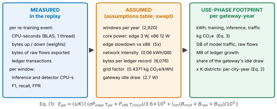
Figure 2.
Top: attack share per window (seed 42). Bottom: F1 on each held-out window for the edge tree (1-day history), seed 42, under four policies; the ticks below the axis mark the windows after which each policy re-trained. The shaded band is the initial training period.
Figure 2.
Top: attack share per window (seed 42). Bottom: F1 on each held-out window for the edge tree (1-day history), seed 42, under four policies; the ticks below the axis mark the windows after which each policy re-trained. The shaded band is the initial training period.
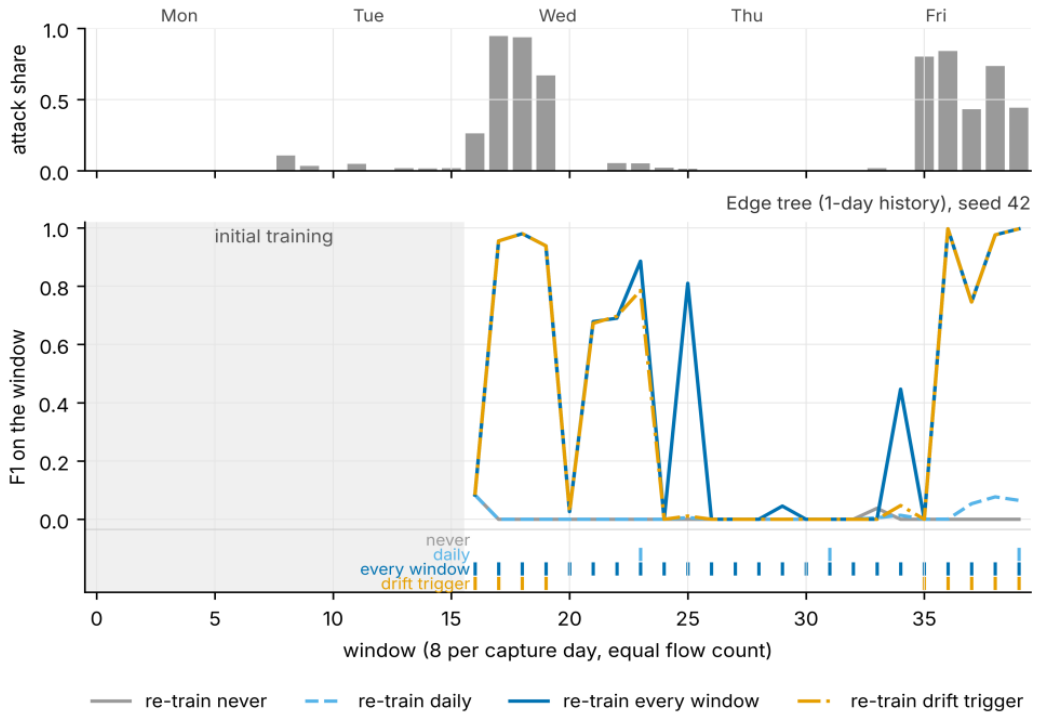
Figure 3.
Stream F1 against estimated energy per gateway-year for every protocol and policy (mean ± 95% CI over five seeds, log x-axis): edge protocols (left) and federated and centralised protocols (right). Labels mark the points on each panel’s detection–energy frontier (each labelled point improves on every cheaper point by more than 0.01 F1): on the left mostly edge-MLP policies and the edge tree’s drift trigger, on the right FedAvg policies and, at the top, the centralised learner’s DDM and every-window points; coincident points share one label.
Figure 3.
Stream F1 against estimated energy per gateway-year for every protocol and policy (mean ± 95% CI over five seeds, log x-axis): edge protocols (left) and federated and centralised protocols (right). Labels mark the points on each panel’s detection–energy frontier (each labelled point improves on every cheaper point by more than 0.01 F1): on the left mostly edge-MLP policies and the edge tree’s drift trigger, on the right FedAvg policies and, at the top, the centralised learner’s DDM and every-window points; coincident points share one label.
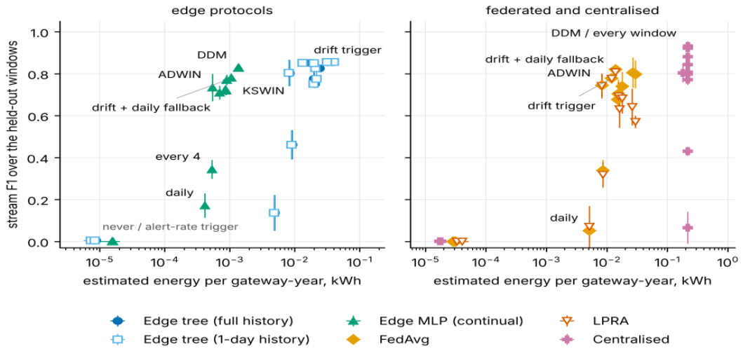
Figure 4.
Where the estimated energy goes under re-training every window: training on the gateway, training in the cloud (per-gateway share), inference, and network traffic (model weights, raw flows and ledger records).
Figure 4.
Where the estimated energy goes under re-training every window: training on the gateway, training in the cloud (per-gateway share), inference, and network traffic (model weights, raw flows and ledger records).
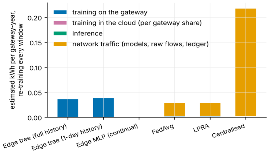
Figure 5.
(a) kg CO2e per city-year against the number of districts, re-training every window, with the same gateways idling as the baseline; (b) ledger growth per year under the three anchoring designs for FedAvg and the two that apply to the edge tree (K = 5).
Figure 5.
(a) kg CO2e per city-year against the number of districts, re-training every window, with the same gateways idling as the baseline; (b) ledger growth per year under the three anchoring designs for FedAvg and the two that apply to the edge tree (K = 5).
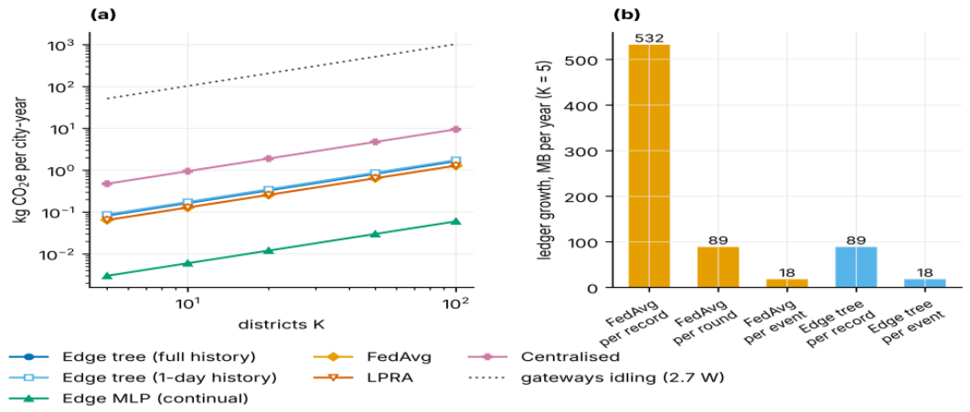
Figure 6.
Sensitivity of the FedAvg scenario energy (re-training every window) to each assumption; bars span the low–high range, the tick is the default.
Figure 6.
Sensitivity of the FedAvg scenario energy (re-training every window) to each assumption; bars span the low–high range, the tick is the default.
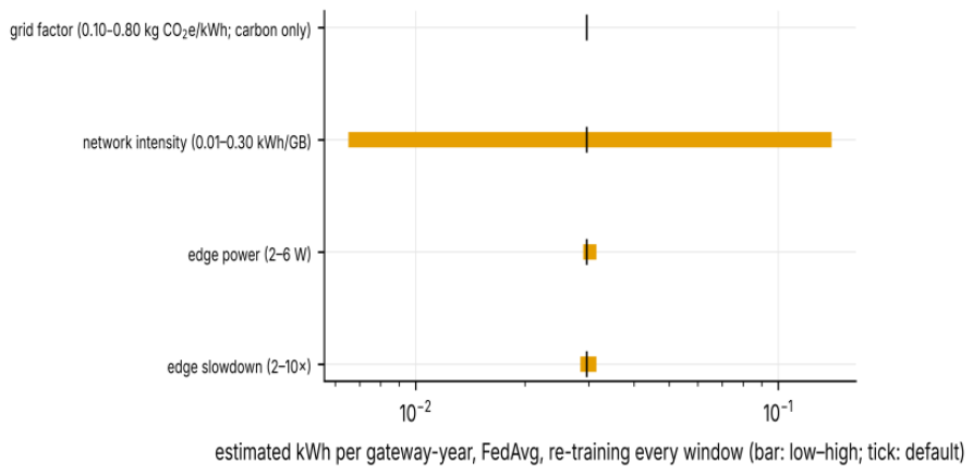
Figure 7.
CSE-CIC-IDS2018. Top: attack share per window (seed 42). Bottom: F1 on each held-out window for the edge tree (1-day history), seed 42, under four policies; the ticks mark the windows after which each policy re-trained. The drift trigger fires only inside the two volumetric blocks or on the window just after them.
Figure 7.
CSE-CIC-IDS2018. Top: attack share per window (seed 42). Bottom: F1 on each held-out window for the edge tree (1-day history), seed 42, under four policies; the ticks mark the windows after which each policy re-trained. The drift trigger fires only inside the two volumetric blocks or on the window just after them.
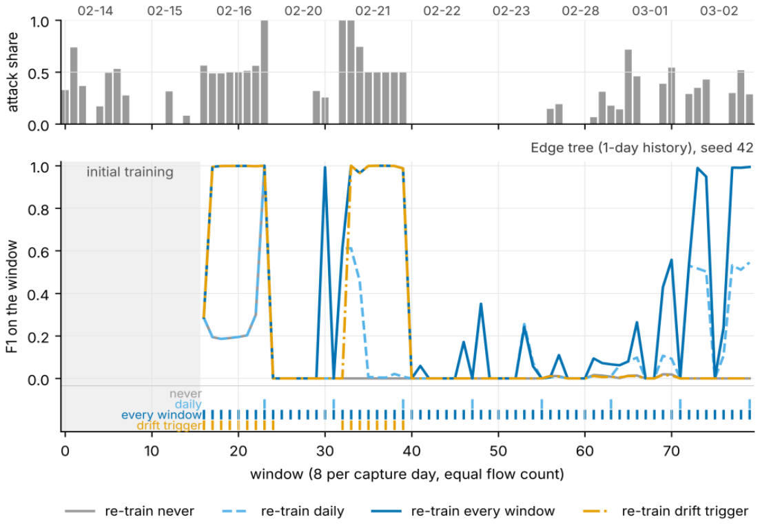

Table 1.
What this paper adds to the previous study [11].
Table 1.
What this paper adds to the previous study [11].
| Aspect | Previous study [11] | This paper |
| Question | does the four-layer architecture detect, federate and anchor, and at what latency and inference-energy cost | what keeping its detector useful costs each year of operation, and which choices move that cost |
| Evaluation | per capture day; one chronological experiment (train three days, test two) | window-by-window replay with twelve re-training policies on two captures (24 + 64 held-out windows) |
| Federated protocols | FedAvg and LPRA on a fixed split, with simulated poisoning | FedAvg and LPRA re-trained on a stream; screen behaviour under benign novelty |
| Cost accounting | inference energy of the deployed tree | re-training CPU, model traffic, raw-flow export, ledger records and detector cost per event, annualised (Equation (1)), with the energy assumptions swept and combined |
| Provenance | one anchor per record on Fabric | per-record, per-round and per-event anchoring with measured Merkle cost |
| Output | detection, latency and throughput figures | use-phase energy, carbon, traffic and storage per gateway-year and per city-year; levers and a tender checklist |
| Questions answered here, not in [11] | — | whether re-training cadence is constrained by its energy (no, within the boundary modelled); whether a label-free trigger can replace a clock (on one capture, not the other); whether the poisoning screen survives benign novelty (not under frequent small updates); which part of the footprint a municipality can move |
Table 2.
The capture week as windows (seed 42): flows, the range of the attack share over the day’s eight windows, and the attack families each day introduces for the first time. The other seeds differ in the third decimal of the shares.
Table 2.
The capture week as windows (seed 42): flows, the range of the attack share over the day’s eight windows, and the attack families each day introduces for the first time. The other seeds differ in the third decimal of the shares.
| Day | Windows | Flows | Attack share (min–max per window) | Families first seen |
| Monday | 0–7 | 160,000 | 0.000–0.000 | (none new) |
| Tuesday | 8–15 | 160,000 | 0.000–0.107 | FTP-Patator, SSH-Patator |
| Wednesday | 16–23 | 160,000 | 0.000–0.947 | DoS Hulk, DoS Slowhttptest, DoS slowloris, DoS GoldenEye, Heartbleed |
| Thursday | 24–31 | 160,000 | 0.000–0.022 | Web Attack Brute Force, Web Attack SQL Injection, Web Attack XSS, Infiltration |
| Friday | 32–39 | 160,000 | 0.002–0.842 | Bot, PortScan, DDoS |
Table 3.
Protocols. K = 5 districts; R = 5 rounds per re-training event for the federated protocols.
Table 3.
Protocols. K = 5 districts; R = 5 rounds per re-training event for the federated protocols.
| Protocol | Model | Re-training computation | Crosses the boundary | Ledger tx per re-training |
| Edge tree (full history) | depth-8 decision tree per district | refit on the district’s whole history | nothing | K |
| Edge tree (1-day history) | same | refit on the district’s last 160,000 flows | nothing | K |
| Edge MLP (continual) | MLP(32,16) per district | partial_fit, 2 epochs over the flows since the last re-training | nothing | K |
| FedAvg | one global MLP(32,16) | R rounds, each 2 local epochs over the new flows, weighted averaging | weights up and down | R·(K+1) |
| LPRA | FedAvg + the two-stage screen of [11] | same, plus the screen | same | same, with the accept/quarantine decision |
| Centralised | one MLP(32,16) in the cloud | 10 epochs over the pooled new flows | raw flows: 77 × 4 B + 1 B per flow | 1 |
Table 4.
Re-training policies.
| Policy | Rule | Needs labels |
| never | the model trained once on the initial period (the deploy-and-forget detector of [11]) | no |
| daily / every 4 / every 2 / every window | after every 8th, 4th, 2nd, 1st window | no |
| alert-rate trigger | re-train when the detector’s own alert rate moves by more than 0.05 from the previous window | no |
| drift trigger | re-train when the window’s standardised feature-mean vector lies farther from the initial-period reference than the mean plus three standard deviations (SD) of the initial windows’ own distances | no |
| drift trigger + daily fallback | re-train when the drift trigger fires or eight flow-count windows have passed since the last re-training | no |
| F1 < 0.5 (reference) | re-train when the true F1 on the window just scored fell below 0.5 (a label-using reference policy, not deployable because it needs the true labels of the window just scored; it reacts after a miss, so it is not an upper bound) | yes |
| ADWIN / KSWIN | standard drift detectors on a per-flow feature statistic (Section 4.2); re-train after a window in which the detector signalled | no |
| DDM | standard drift detector on the deployed model’s 0/1 error on every flow (Section 4.2) | yes |
Table 5.
Use-phase accounting assumptions, their sources and the ranges swept in Section 4.7.
Table 5.
Use-phase accounting assumptions, their sources and the ranges swept in Section 4.7.
| Assumption | Default | Source / rationale | Swept |
| Windows per year | 2,920 | 8 per day × 365; the year repeats the capture | — |
| x86 host power while one core works (W) | 12 | energy estimate of [11] | — |
| Edge gateway power while one core works (W) | 3 | energy estimate of [11]; Pi 4 measured 2.4–2.9 W idle, 6.7–7.3 W four-core load [40] | 2–6 |
| Edge slowdown vs. this x86 core (×) | 5 | assumed; bracketed by the 2–10× sweep | 2–10 |
| Network electricity intensity (kWh/GB) | 0.06 | Aslan et al. 2018, fixed line, 2015 [41] | 0.01–0.30 |
| Ledger bytes per anchored record (B) | 6,076 | Fabric measurement of [11] | — |
| Grid emission factor (kg CO2e/kWh) | 0.4371 | Thailand Greenhouse Gas Management Organization (TGO), announced 28 May 2025 (value for 2022) [50] | 0.10–0.80 |
| Gateway idle draw (W) | 2.7 | literature range 2.4–2.9 W [40] | — |
Table 6.
Stream F1 over the 24 held-out windows (one confusion matrix over the stream), mean ± 95% confidence interval (CI) over five seeds; entries are rounded to three decimals and intervals are not clipped at zero.
Table 6.
Stream F1 over the 24 held-out windows (one confusion matrix over the stream), mean ± 95% confidence interval (CI) over five seeds; entries are rounded to three decimals and intervals are not clipped at zero.
| Protocol | never | daily | every 4 | every 2 | every window | drift trigger | F1 < 0.5 (ref.) |
| Edge tree (full history) | 0.005 ± 0.001 | 0.137 ± 0.085 | 0.462 ± 0.070 | 0.751 ± 0.010 | 0.856 ± 0.006 | 0.852 ± 0.010 | 0.776 ± 0.036 |
| Edge tree (1-day history) | 0.005 ± 0.001 | 0.137 ± 0.085 | 0.461 ± 0.069 | 0.752 ± 0.010 | 0.856 ± 0.006 | 0.852 ± 0.010 | 0.776 ± 0.036 |
| Edge MLP (continual) | 0.000 ± 0.001 | 0.172 ± 0.058 | 0.344 ± 0.045 | 0.726 ± 0.003 | 0.830 ± 0.013 | 0.710 ± 0.033 | 0.720 ± 0.022 |
| FedAvg | 0.000 ± 0.000 | 0.052 ± 0.083 | 0.339 ± 0.051 | 0.704 ± 0.069 | 0.798 ± 0.066 | 0.779 ± 0.015 | 0.677 ± 0.019 |
| LPRA | 0.000 ± 0.000 | 0.071 ± 0.098 | 0.318 ± 0.061 | 0.693 ± 0.067 | 0.571 ± 0.030 | 0.776 ± 0.021 | 0.631 ± 0.089 |
| Centralised | 0.001 ± 0.001 | 0.066 ± 0.076 | 0.431 ± 0.022 | 0.772 ± 0.025 | 0.933 ± 0.008 | 0.807 ± 0.024 | 0.804 ± 0.045 |
Table 7.
Mean F1 over the 24 held-out windows (each window weighted equally), mean ± 95% CI over five seeds.
Table 7.
Mean F1 over the 24 held-out windows (each window weighted equally), mean ± 95% CI over five seeds.
| Protocol | never | daily | every 4 | every 2 | every window | drift trigger | F1 < 0.5 (ref.) |
| Edge tree (full history) | 0.006 ± 0.002 | 0.057 ± 0.032 | 0.232 ± 0.024 | 0.337 ± 0.013 | 0.410 ± 0.015 | 0.376 ± 0.007 | 0.376 ± 0.016 |
| Edge tree (1-day history) | 0.006 ± 0.002 | 0.057 ± 0.032 | 0.231 ± 0.024 | 0.338 ± 0.014 | 0.411 ± 0.015 | 0.376 ± 0.007 | 0.375 ± 0.016 |
| Edge MLP (continual) | 0.000 ± 0.000 | 0.068 ± 0.018 | 0.134 ± 0.024 | 0.281 ± 0.018 | 0.367 ± 0.024 | 0.315 ± 0.010 | 0.320 ± 0.009 |
| FedAvg | 0.000 ± 0.000 | 0.022 ± 0.034 | 0.135 ± 0.027 | 0.274 ± 0.035 | 0.348 ± 0.025 | 0.319 ± 0.006 | 0.301 ± 0.014 |
| LPRA | 0.000 ± 0.000 | 0.030 ± 0.039 | 0.126 ± 0.027 | 0.265 ± 0.034 | 0.196 ± 0.014 | 0.315 ± 0.010 | 0.280 ± 0.033 |
| Centralised | 0.001 ± 0.001 | 0.029 ± 0.030 | 0.186 ± 0.010 | 0.341 ± 0.028 | 0.498 ± 0.018 | 0.333 ± 0.005 | 0.400 ± 0.021 |
Table 8.
Stream false-positive rate under each re-training policy that fires (never and the alert-rate trigger, which never fires on this stream, omitted; mean over five seeds).
Table 8.
Stream false-positive rate under each re-training policy that fires (never and the alert-rate trigger, which never fires on this stream, omitted; mean over five seeds).
| Protocol | daily | every 4 | every 2 | every window | drift trigger | F1 < 0.5 (ref.) |
| Edge tree (full history) | 0.0023 | 0.0050 | 0.0037 | 0.0024 | 0.0040 | 0.0023 |
| Edge tree (1-day history) | 0.0023 | 0.0050 | 0.0037 | 0.0024 | 0.0040 | 0.0023 |
| Edge MLP (continual) | 0.0190 | 0.0230 | 0.0211 | 0.0203 | 0.1401 | 0.0172 |
| FedAvg | 0.0210 | 0.0130 | 0.0081 | 0.0099 | 0.0590 | 0.0069 |
| LPRA | 0.0188 | 0.0122 | 0.0079 | 0.0081 | 0.0522 | 0.0060 |
| Centralised | 0.0095 | 0.0116 | 0.0070 | 0.0059 | 0.0475 | 0.0071 |
Table 9.
Re-training triggers compared: the feature-mean drift trigger of this paper, ADWIN and KSWIN (label-free) and DDM and the F1-threshold reference policy (label-using). Stream F1 (mean ± 95% CI), FPR, re-trainings per year, re-training CPU-hours and the detector’s own CPU-hours per gateway-year.
Table 9.
Re-training triggers compared: the feature-mean drift trigger of this paper, ADWIN and KSWIN (label-free) and DDM and the F1-threshold reference policy (label-using). Stream F1 (mean ± 95% CI), FPR, re-trainings per year, re-training CPU-hours and the detector’s own CPU-hours per gateway-year.
| Protocol | Trigger | stream F1 | FPR | re-trainings / yr | CPU h / gw-yr | detector CPU h / gw-yr |
| Edge tree (1-day history) | drift trigger | 0.852 ± 0.010 | 0.0040 | 1,095 | 0.856 | 0.0000 |
| Edge tree (1-day history) | ADWIN | 0.804 ± 0.063 | 0.0027 | 730 | 0.520 | 0.0012 |
| Edge tree (1-day history) | KSWIN | 0.827 ± 0.011 | 0.0024 | 1,728 | 1.333 | 0.0121 |
| Edge tree (1-day history) | DDM | 0.856 ± 0.006 | 0.0025 | 2,847 | 2.023 | 0.0015 |
| Edge tree (1-day history) | F1 < 0.5 (reference) | 0.776 ± 0.036 | 0.0023 | 1,265 | 1.408 | 0.0000 |
| Edge MLP (continual) | drift trigger | 0.710 ± 0.033 | 0.1401 | 1,095 | 0.019 | 0.0000 |
| Edge MLP (continual) | ADWIN | 0.735 ± 0.065 | 0.0343 | 730 | 0.017 | 0.0010 |
| Edge MLP (continual) | KSWIN | 0.781 ± 0.010 | 0.0195 | 1,728 | 0.017 | 0.0104 |
| Edge MLP (continual) | DDM | 0.828 ± 0.014 | 0.0224 | 2,847 | 0.018 | 0.0016 |
| Edge MLP (continual) | F1 < 0.5 (reference) | 0.720 ± 0.022 | 0.0172 | 1,606 | 0.018 | 0.0000 |
| FedAvg | drift trigger | 0.779 ± 0.015 | 0.0590 | 1,095 | 0.101 | 0.0000 |
| FedAvg | ADWIN | 0.745 ± 0.053 | 0.0115 | 730 | 0.087 | 0.0011 |
| FedAvg | KSWIN | 0.740 ± 0.069 | 0.0074 | 1,728 | 0.092 | 0.0111 |
| FedAvg | DDM | 0.806 ± 0.072 | 0.0096 | 2,677 | 0.101 | 0.0016 |
| FedAvg | F1 < 0.5 (reference) | 0.677 ± 0.019 | 0.0069 | 1,436 | 0.101 | 0.0000 |
| Centralised | drift trigger | 0.807 ± 0.024 | 0.0475 | 1,095 | 0.121 | 0.0000 |
| Centralised | ADWIN | 0.798 ± 0.040 | 0.0090 | 730 | 0.079 | 0.0011 |
| Centralised | KSWIN | 0.882 ± 0.038 | 0.0062 | 1,728 | 0.078 | 0.0113 |
| Centralised | DDM | 0.922 ± 0.034 | 0.0059 | 2,725 | 0.080 | 0.0016 |
| Centralised | F1 < 0.5 (reference) | 0.804 ± 0.045 | 0.0071 | 1,119 | 0.101 | 0.0000 |
Table 10.
Measured upkeep, annualised from the capture week to 2,920 windows per year (K = 5; CPU-hours on the x86 host, BLAS single-threaded; mean over five seeds; for the capped tree the replay’s own average while the history is still filling, the text below the table gives the full-cap figure; ledger bytes are not in the model-traffic column and are added, at one K-th per gateway, when energy is computed), under re-training every window and under the drift trigger.
Table 10.
Measured upkeep, annualised from the capture week to 2,920 windows per year (K = 5; CPU-hours on the x86 host, BLAS single-threaded; mean over five seeds; for the capped tree the replay’s own average while the history is still filling, the text below the table gives the full-cap figure; ledger bytes are not in the model-traffic column and are added, at one K-th per gateway, when energy is computed), under re-training every window and under the drift trigger.
| Protocol | Policy | re-trainings / yr | CPU h / gw-yr | model GB / gw-yr | raw GB / gw-yr | ledger tx / yr (city) |
| Edge tree (full history) | every window | 2,920 | 2.451 | 0.000 | 0.00 | 14,600 |
| Edge tree (1-day history) | every window | 2,920 | 2.605 | 0.000 | 0.00 | 14,600 |
| Edge MLP (continual) | every window | 2,920 | 0.020 | 0.000 | 0.00 | 14,600 |
| FedAvg | every window | 2,920 | 0.125 | 0.355 | 0.00 | 87,600 |
| LPRA | every window | 2,920 | 0.124 | 0.355 | 0.00 | 87,600 |
| Centralised | every window | 2,920 | 0.116 | 0.000 | 3.61 | 2,920 |
| Edge tree (full history) | drift trigger | 1,095 | 1.131 | 0.000 | 0.00 | 5,475 |
| Edge tree (1-day history) | drift trigger | 1,095 | 0.856 | 0.000 | 0.00 | 5,475 |
| Edge MLP (continual) | drift trigger | 1,095 | 0.019 | 0.000 | 0.00 | 5,475 |
| FedAvg | drift trigger | 1,095 | 0.101 | 0.133 | 0.00 | 32,850 |
| LPRA | drift trigger | 1,095 | 0.105 | 0.133 | 0.00 | 32,850 |
| Centralised | drift trigger | 1,095 | 0.121 | 0.000 | 3.61 | 1,095 |
Table 11.
Estimated edge-class scenario per gateway-year (assumptions of Table 5: 3 W one-core power, 5× slowdown, 0.06 kWh/GB, 0.4371 kg CO2e/kWh, 2.7 W idle baseline). Share = upkeep energy as a percentage of the gateway’s idle draw.
Table 11.
Estimated edge-class scenario per gateway-year (assumptions of Table 5: 3 W one-core power, 5× slowdown, 0.06 kWh/GB, 0.4371 kg CO2e/kWh, 2.7 W idle baseline). Share = upkeep energy as a percentage of the gateway’s idle draw.
| Protocol | Policy | kWh training | kWh inference | kWh traffic | kWh total / gw-yr | kg CO2e / gw-yr | share % |
| Edge tree (full history) | every window | 0.0368 | 0.00001 | 0.0011 | 0.0378 | 0.0165 | 0.16 |
| Edge tree (1-day history) | every window | 0.0391 | 0.00001 | 0.0011 | 0.0401 | 0.0175 | 0.17 |
| Edge MLP (continual) | every window | 0.0003 | 0.00002 | 0.0011 | 0.0014 | 0.0006 | 0.01 |
| FedAvg | every window | 0.0019 | 0.00003 | 0.0277 | 0.0296 | 0.0129 | 0.13 |
| LPRA | every window | 0.0019 | 0.00003 | 0.0277 | 0.0296 | 0.0129 | 0.13 |
| Centralised | every window | 0.0014 | 0.00002 | 0.2168 | 0.2182 | 0.0954 | 0.92 |
| Edge tree (full history) | drift trigger | 0.0170 | 0.00001 | 0.0004 | 0.0174 | 0.0076 | 0.07 |
| Edge tree (1-day history) | drift trigger | 0.0128 | 0.00001 | 0.0004 | 0.0133 | 0.0058 | 0.06 |
| Edge MLP (continual) | drift trigger | 0.0003 | 0.00002 | 0.0004 | 0.0007 | 0.0003 | 0.00 |
| FedAvg | drift trigger | 0.0015 | 0.00004 | 0.0104 | 0.0119 | 0.0052 | 0.05 |
| LPRA | drift trigger | 0.0016 | 0.00003 | 0.0104 | 0.0120 | 0.0052 | 0.05 |
| Centralised | drift trigger | 0.0015 | 0.00002 | 0.2166 | 0.2181 | 0.0953 | 0.92 |
Table 12.
Anchoring granularity for FedAvg (K = 5): transactions and ledger growth per year, proof size, and the measured Merkle cost per batch.
Table 12.
Anchoring granularity for FedAvg (K = 5): transactions and ledger growth per year, proof size, and the measured Merkle cost per batch.
| Policy | Anchoring | Batch | tx / yr | MB / yr | Reduction % | Proof B | Root+proof µs | Verify µs |
| every window | per-record | 1 | 87,600 | 532 | 0 | 0 | 0.2 | 0.1 |
| every window | per-round | 6 | 14,600 | 89 | 83 | 96 | 9.9 | 1.9 |
| every window | per-event | 30 | 2,920 | 18 | 97 | 160 | 38.2 | 3.2 |
| drift trigger | per-record | 1 | 32,850 | 200 | 0 | 0 | 0.2 | 0.1 |
| drift trigger | per-round | 6 | 5,475 | 33 | 83 | 96 | 9.9 | 1.9 |
| drift trigger | per-event | 30 | 1,095 | 7 | 97 | 160 | 38.2 | 3.2 |
Table 13.
One-at-a-time sensitivity: scenario kWh per gateway-year under re-training every window for three protocols at the low, default and high value of each assumption; tree* = edge tree (1-day history).
Table 13.
One-at-a-time sensitivity: scenario kWh per gateway-year under re-training every window for three protocols at the low, default and high value of each assumption; tree* = edge tree (1-day history).
| Assumption | low | tree* | FedAvg | central | default | tree* | FedAvg | central | high | tree* | FedAvg | central |
| edge slowdown (x) | 2 | 0.0167 | 0.0285 | 0.2182 | 5 | 0.0401 | 0.0296 | 0.2182 | 10 | 0.0792 | 0.0315 | 0.2182 |
| edge power (W) | 2 | 0.0271 | 0.0290 | 0.2182 | 3 | 0.0401 | 0.0296 | 0.2182 | 6 | 0.0792 | 0.0315 | 0.2182 |
| network intensity (kWh/GB) | 0.01 | 0.0393 | 0.0065 | 0.0375 | 0.06 | 0.0401 | 0.0296 | 0.2182 | 0.3 | 0.0444 | 0.1404 | 1.0852 |
| grid factor (kg CO2e/kWh) | 0.1 | 0.0401 | 0.0296 | 0.2182 | 0.4371 | 0.0401 | 0.0296 | 0.2182 | 0.8 | 0.0401 | 0.0296 | 0.2182 |
Table 14.
Combined energy scenarios: estimated upkeep per gateway-year under re-training every window when every energy assumption is moved at once: best case (2 W, 2×, 0.01 kWh/GB, 8 windows a day), default (Table 5) and worst case (6 W, 10×, 0.30 kWh/GB, 24 windows a day). Share = percentage of the gateway’s idle draw, held at 2.7 W.
Table 14.
Combined energy scenarios: estimated upkeep per gateway-year under re-training every window when every energy assumption is moved at once: best case (2 W, 2×, 0.01 kWh/GB, 8 windows a day), default (Table 5) and worst case (6 W, 10×, 0.30 kWh/GB, 24 windows a day). Share = percentage of the gateway’s idle draw, held at 2.7 W.
| Protocol | best kWh | share % | default kWh | share % | worst kWh | share % |
| Edge tree (1-day history) | 0.0106 | 0.04 | 0.0401 | 0.17 | 0.4850 | 2.05 |
| Edge MLP (continual) | 0.0003 | 0.00 | 0.0014 | 0.01 | 0.0198 | 0.08 |
| FedAvg | 0.0051 | 0.02 | 0.0296 | 0.13 | 0.4384 | 1.85 |
| LPRA | 0.0051 | 0.02 | 0.0296 | 0.13 | 0.4382 | 1.85 |
| Centralised | 0.0375 | 0.16 | 0.2182 | 0.92 | 3.2558 | 13.77 |
Table 15.
The CSE-CIC-IDS2018 capture as windows (seed 42): flows, the range of the attack share over the day’s eight windows, and the attack families each day introduces for the first time.
Table 15.
The CSE-CIC-IDS2018 capture as windows (seed 42): flows, the range of the attack share over the day’s eight windows, and the attack families each day introduces for the first time.
| Day | Windows | Flows | Attack share (min–max per window) | Families first seen |
| Wed 14 Feb | 0–7 | 160,000 | 0.000–0.738 | SSH-Bruteforce, FTP-BruteForce |
| Thu 15 Feb | 8–15 | 160,000 | 0.000–0.314 | DoS GoldenEye, DoS Slowloris |
| Fri 16 Feb | 16–23 | 160,000 | 0.488–0.999 | DoS Hulk, DoS SlowHTTPTest |
| Tue 20 Feb | 24–31 | 160,000 | 0.000–0.319 | DDoS LOIC-HTTP |
| Wed 21 Feb | 32–39 | 160,000 | 0.497–1.000 | DDoS HOIC, DDoS LOIC-UDP |
| Thu 22 Feb | 40–47 | 160,000 | 0.000–0.002 | Brute Force XSS, SQL Injection, Brute Force Web |
| Fri 23 Feb | 48–55 | 160,000 | 0.000–0.003 | (none new) |
| Wed 28 Feb | 56–63 | 159,989 | 0.000–0.311 | Infiltration |
| Thu 1 Mar | 64–71 | 159,991 | 0.000–0.716 | (none new) |
| Fri 2 Mar | 72–79 | 160,000 | 0.000–0.518 | Bot |
Table 16.
CSE-CIC-IDS2018: stream F1 over the 64 held-out windows, mean ± 95% CI over five seeds.
| Protocol | never | daily | every 4 | every 2 | every window | drift trigger | F1 < 0.5 (ref.) |
| Edge tree (full history) | 0.257 ± 0.105 | 0.348 ± 0.127 | 0.617 ± 0.062 | 0.742 ± 0.030 | 0.814 ± 0.013 | 0.695 ± 0.018 | 0.717 ± 0.057 |
| Edge tree (1-day history) | 0.257 ± 0.105 | 0.374 ± 0.105 | 0.628 ± 0.056 | 0.749 ± 0.028 | 0.820 ± 0.012 | 0.694 ± 0.018 | 0.713 ± 0.062 |
| Edge MLP (continual) | 0.448 ± 0.002 | 0.417 ± 0.036 | 0.643 ± 0.030 | 0.756 ± 0.019 | 0.802 ± 0.009 | 0.663 ± 0.031 | 0.787 ± 0.017 |
| FedAvg | 0.454 ± 0.002 | 0.418 ± 0.016 | 0.655 ± 0.026 | 0.754 ± 0.010 | 0.773 ± 0.008 | 0.709 ± 0.005 | 0.717 ± 0.053 |
| LPRA | 0.454 ± 0.002 | 0.429 ± 0.010 | 0.648 ± 0.020 | 0.744 ± 0.014 | 0.780 ± 0.021 | 0.709 ± 0.005 | 0.787 ± 0.047 |
| Centralised | 0.452 ± 0.004 | 0.464 ± 0.038 | 0.656 ± 0.016 | 0.741 ± 0.023 | 0.801 ± 0.007 | 0.709 ± 0.022 | 0.740 ± 0.019 |
Table 17.
The drift trigger with a one-day clock fallback (re-train when the trigger fires or after eight flow-count windows without a re-training): stream F1, paired difference to re-training every window (mean and 95% CI over five seeds), and re-trainings per year, on both streams.
Table 17.
The drift trigger with a one-day clock fallback (re-train when the trigger fires or after eight flow-count windows without a re-training): stream F1, paired difference to re-training every window (mean and 95% CI over five seeds), and re-trainings per year, on both streams.
| Protocol | 2017 F1 | 2017 Δ vs every window | 2017 re-trainings / yr | 2018 F1 | 2018 Δ vs every window | 2018 re-trainings / yr |
| Edge tree (1-day history) | 0.851 | −0.005 [−0.011, +0.001] | 1,217 | 0.740 | −0.080 [−0.117, −0.043] | 1,004 |
| Edge MLP (continual) | 0.770 | −0.059 [−0.076, −0.043] | 1,217 | 0.687 | −0.116 [−0.182, −0.049] | 1,004 |
| FedAvg | 0.820 | +0.022 [−0.040, +0.085] | 1,217 | 0.714 | −0.059 [−0.092, −0.026] | 1,004 |
| Centralised | 0.844 | −0.089 [−0.097, −0.080] | 1,217 | 0.717 | −0.084 [−0.144, −0.024] | 1,004 |
Table 18.
CSE-CIC-IDS2018: measured upkeep, annualised (2,920 windows per year; CPU-hours on the x86 host; mean over five seeds) under re-training every window and under the drift trigger.
Table 18.
CSE-CIC-IDS2018: measured upkeep, annualised (2,920 windows per year; CPU-hours on the x86 host; mean over five seeds) under re-training every window and under the drift trigger.
| Protocol | Policy | re-trainings / yr | CPU h / gw-yr | model GB / gw-yr | raw GB / gw-yr | ledger tx / yr (city) |
| Edge tree (full history) | every window | 2,920 | 2.841 | 0.000 | 0.00 | 14,600 |
| Edge tree (1-day history) | every window | 2,920 | 1.887 | 0.000 | 0.00 | 14,600 |
| Edge MLP (continual) | every window | 2,920 | 0.017 | 0.000 | 0.00 | 14,600 |
| FedAvg | every window | 2,920 | 0.089 | 0.351 | 0.00 | 87,600 |
| LPRA | every window | 2,920 | 0.090 | 0.351 | 0.00 | 87,600 |
| Centralised | every window | 2,920 | 0.079 | 0.000 | 3.56 | 2,920 |
| Edge tree (full history) | drift trigger | 785 | 0.264 | 0.000 | 0.00 | 3,924 |
| Edge tree (1-day history) | drift trigger | 785 | 0.268 | 0.000 | 0.00 | 3,924 |
| Edge MLP (continual) | drift trigger | 785 | 0.006 | 0.000 | 0.00 | 3,924 |
| FedAvg | drift trigger | 785 | 0.031 | 0.094 | 0.00 | 23,542 |
| LPRA | drift trigger | 785 | 0.032 | 0.094 | 0.00 | 23,542 |
| Centralised | drift trigger | 785 | 0.026 | 0.000 | 1.35 | 785 |
Table 19.
The sustainability levers of a smart-city intrusion-detection deployment, from the measured quantities and the scenario of Section 4 (per gateway-year unless stated; K = 5).
Table 19.
The sustainability levers of a smart-city intrusion-detection deployment, from the measured quantities and the scenario of Section 4 (per gateway-year unless stated; K = 5).
| Lever | Choice | Effect (scenario defaults) | Detection effect | Who decides |
| Re-training cadence | never → every window | +0.0401 kWh at most among the edge and federated designs (edge tree); +0.2182 for raw-flow export | stream F1 0.005 → 0.856 (daily: 0.137) | operations (labelling capacity) |
| Trigger instead of clock | drift trigger vs every window | −62.5% re-trainings, −67% CPU-h | F1 0.852 vs 0.856; FPR 0.0024 → 0.0040 (tree), 0.0203 → 0.1401 (edge MLP) | gateway software requirement |
| Where learning happens | raw-flow export vs edge / federated | 0.2182 vs ≤ 0.0401 kWh; 3.61 GB of raw-flow records leave the district vs none | F1 0.933 vs 0.856 | data governance |
| Provenance granularity | per record → per round → per event | ledger 532 → 89 → 18 MB per year; 9.0 GB per year at K = 100 per record; the nodes themselves are always-on infrastructure outside the account (Section 5.2) | none (proof of membership retained) | ledger design |
| Gateway hardware | idle draw 2.7 W | 23.7 kWh per year idling: 1,034 kg CO2e per 100 gateways vs 1.75 kg for keeping their detectors alive | none | procurement |
Disclaimer/Publisher’s Note: The statements, opinions and data contained in all publications are solely those of the individual author(s) and contributor(s) and not of MDPI and/or the editor(s). MDPI and/or the editor(s) disclaim responsibility for any injury to people or property resulting from any ideas, methods, instructions or products referred to in the content. |
© 2026 by the authors. Licensee MDPI, Basel, Switzerland. This article is an open access article distributed under the terms and conditions of the Creative Commons Attribution (CC BY) license.
Copyright: This open access article is published under a Creative Commons CC BY 4.0 license, which permit the free download, distribution, and reuse, provided that the author and preprint are cited in any reuse.