

Submitted:
03 November 2026
Posted:
05 November 2026
You are already at the latest version
Abstract
Neurodegenerative diseases such as Alzheimer disease are commonly studied with struc tural magnetic resonance imaging (MRI), in which whole-brain parcellation provides volu metric measures of brain structures. Atlas-based parcellation takes hours per subject, and deep learning models that accelerate it are limited by the cost of volumetric annotation. Self-supervised pretraining addresses this, but is usually demonstrated on large external unlabeled corpora that many laboratories do not have. We ask whether pretraining on the same modest cohort that supplies the labels helps, and at which annotation budgets. Using 148 T1-weighted volumes from OASIS-3 (one per participant, Clinical Dementia Rating 0–2) and 27 FreeSurfer-derived structures, a 3D U-Net was pretrained by masked-volume reconstruction on each cross-validation fold’s training split and fine-tuned with 10, 25, 50 and 104 labeled subjects. The gain from pretraining was largest when annotation was scarce: +0.0610 Dice at 25 labeled subjects against +0.0143 at 104. Under a corrected resampled t-test for dependent folds, it was significant at 25 (p = 0.005) and 10 (p = 0.039), but not at 50 or 104. With 25 labeled subjects, the pretrained model reached 95.7% of the Dice of a randomly initialized model trained on 104. Segmentation accuracy showed no detectable dependence on dementia severity once scanner model was accounted for, whereas scanner model had a large effect (Cohen’s d = 0.99 among cognitively normal participants), and the pretraining benefit did not vary detectably with severity. When annotation is the constraint, pretraining on the unlabeled cohort before annotating a fraction of it is the better use of effort.
Keywords:
brain MRI
; semantic segmentation
; self-supervised learning
; label efficiency
; whole-brain parcellation
; 3D U-Net
; RRID:SCR_003430
1. Introduction
Whole-brain parcellation can be simply defined as the process in which every voxel of a structural MRI volume is assigned to an anatomical structure, such as the hippocampus, cortex, and so on. This step is an important process in quantitative neuroimaging and in the diagnosis of brain diseases. Volumetric morphometry, atrophy tracking, and most region-of-interest analyses always begin by segmenting the brain into labeled compartments, and almost every downstream measurement depends on this initial labeling being accurate. If any error is introduced at this stage, it propagates into every analysis done on the basis of the initial analysis. Many tools are used for this task, but the most prominent are atlas-based and Bayesian methods, which work by comparing a new scan against a reference atlas of known anatomy and using probabilistic reasoning to assign the most likely label to each voxel [1]. The FreeSurfer aseg pipeline is one of the established tools based on these atlas-based and Bayesian methods and is found to be widely used in brain parcellation [1,2]. Although these tools are accurate and well validated, they are time-consuming, as they take hours of computation per subject’s MRI scan [3].
This computational cost has motivated the search for faster alternatives that are capable of preserving the accuracy at a fraction of the runtime. One of the most widely used alternatives is learning-based models, such as convolutional parcellation networks, which have successfully reduced computation time from hours to about a minute [3]. However, these models require large annotated cohorts. This annotation, or labeling, is done either manually or generated automatically, and in both cases the process is slow, time-consuming, and expensive [1,3]. Even when labeling is automatic, it must still be verified manually. So, although the models themselves are readily available, labeled data remains limited.
A widely adopted alternative to address the scarcity of labeled data in medical imaging is self-supervised learning. In this type of learning, the model learns useful representations from unlabeled data before being trained on a smaller labeled dataset [4,5]. However, it is found that this approach typically relies on large amounts of external unlabeled data collected from different sites [6]. In cases of limited labeled data, unlabeled data, and funding, the performance of this method needs to be determined, as it assumes pretraining on a large amount of data.
The purpose of this study is to address a real-world problem in which a single laboratory can typically assemble only a small number of images, and annotating even a few of them costs a substantial amount of money. As mentioned earlier, a common remedy for this problem is self-supervised pretraining [7], but it is usually evaluated and demonstrated on large external corpora [6]. This paper therefore evaluates masked-reconstruction pretraining [5] under deliberately unfavorable conditions, which we regard as the worst realistic case for this method. The major research question is whether the gains from pretraining justify its additional computational cost and effort.
In this paper, the study is framed as a controlled characterization rather than a method proposal. Every comparison is made on the same subjects and the same folds and differs from its counterpart in exactly one variable, so the question is when and where pretraining helps, not whether a new architecture outperforms existing ones. The main contributions are fourfold. First, a fold-matched label-efficiency study across four annotation budgets in which pretraining is performed per fold on training subjects only, so that the cross-validation estimate remains uncontaminated. Second, evidence that the benefit is concentrated in the low-annotation regime, and that it survives a statistical correction for the dependence between folds only there. Third, a structure-wise analysis showing that the gain is not explained by structure size. Fourth, a subject-level analysis of 148 participants spanning the range from cognitively normal to moderate dementia, showing no detectable dependence of segmentation accuracy on disease severity once scanner is accounted for, a substantially larger effect of acquisition hardware, and no detectable variation of the pretraining benefit with clinical severity.
2. Related Work
2.1. Atlas-Based and Learned Parcellation
The reference approach to whole-brain segmentation is atlas-based. The FreeSurfer aseg pipeline [1] registers each subject to a probabilistic atlas built from manually labeled brains and resolves labels under a Markov random field prior. It remains the de facto standard and, as in the present study, frequently supplies the labels on which learned methods are trained. SAMSEG later removed the dependence on a fixed acquisition protocol [8]. Both are well validated, but the full FreeSurfer pipeline requires hours per subject [3], and the reliability of both varies by structure [2].
Learned replacements descend from the encoder–decoder network of Ronneberger et al. [9] and its volumetric successors [10,11], more recently extended with transformer backbones [12]. nnU-Net [13] showed that a self-configuring pipeline, which adapts preprocessing, network topology, patch size and batch size to each dataset, outperformed most specialized solutions across a wide range of segmentation tasks. QuickNAT [14] trains on labels generated by an existing automated pipeline before fine-tuning on a smaller manually annotated set, and FastSurfer [3] extends this into a complete pipeline. SynthSeg [15] instead trains on images synthesized from label maps and generalizes across acquisition protocols without retraining, while SLANT [16], AssemblyNet [17] and DeepNAT [18] rely on spatially localized networks, large ensembles and hierarchical segmentation, respectively. We do not propose a new architecture: a deliberately standard 3D U-Net is used so that the variable under study is initialization rather than model design.
2.2. Self-Supervised Pretraining for Volumetric Medical Imaging
Models Genesis [4] established image restoration as an effective pretext task for 3D medical volumes. Masked autoencoding [5] showed in natural images that reconstructing a large hidden fraction of the input forces a model to learn semantics rather than local interpolation, and SimMIM [19] showed that a plain pixel-regression head suffices. Tang et al. [6] combined masked inpainting with contrastive and rotation objectives to pretrain the Swin transformer encoder of Swin UNETR [20] on several thousand CT volumes. Contrastive and view-alignment methods [21,22], 3D adaptations of pretext tasks such as rotation prediction and jigsaw puzzles [23], and context restoration [24] form alternative families, and in one small-scale comparison on medical image classification, masked-image pretraining was more robust than contrastive pretraining to reductions in training-set size [7]. Closest to the present work, Zhou et al. [25] pretrained masked autoencoders on the training set of the target task itself and reported gains for medical image classification and segmentation.
The major point that distinguishes the present study from most of this work is scale and provenance rather than method. Most of the works above pretrain on external corpora that are typically much larger than ours, roughly fifty times larger in the case of Tang et al. [6]. Relative to self pre-training [25], we target whole-brain parcellation with a convolutional network, pretrain on approximately 104 volumes per fold drawn from the same cohort that supplies the supervision, and report what that provides at each of four annotation budgets. Because published figures derive from different cohorts, label sets, averaging conventions and reference standards, we draw no direct numerical comparison with them; all comparisons in this paper are internal and fold-matched.
3. Materials and Methods
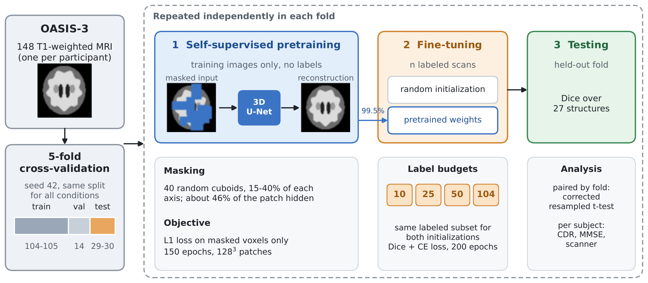
Figure 1 summarizes the study design. Further implementation detail is given in the Supporting Information (Section S1).
3.1. Dataset and Label Set
We used T1-weighted structural MRI volumes from the third release of the Open Access Series of Imaging Studies (OASIS-3) [26], a longitudinal study of normal aging and Alzheimer disease that extends the earlier cross-sectional OASIS release [27]. The data were obtained from the NITRC Image Repository (NITRC-IR; https://www.nitrc.org, RRID:SCR_003430). We retained a single imaging session per participant, so the 148 volumes correspond to 148 distinct individuals and every cross-validation split is subject-disjoint by construction.
Cohort characteristics are summarized in Table 1. Participants ranged from cognitively normal to moderate dementia: by global Clinical Dementia Rating (CDR) [28], 36 participants () carried measurable impairment, so the cohort contains substantial atrophy and ventricular enlargement as well as healthy anatomy. All images were acquired on Siemens scanners, 147 of them at 3 T. The OASIS-3 reference [26] lists the scanner models and sequence types, and per-scan acquisition parameters for all scanners are distributed with the data.
Each volume was accompanied by a whole-brain parcellation produced with the FreeSurfer aseg pipeline [1], which served as the reference standard throughout. This reference is itself the output of an automated method rather than manual expert annotation (Section 6). Images and label maps were supplied in FreeSurfer conformed space, voxels at 1 mm isotropic resolution. We retained 28 classes (27 anatomical structures plus background), chosen so that every lateralized structure appears on both sides: cerebral white matter and cortex, cerebellar white matter and cortex, the lateral, third and fourth ventricles, thalamus, caudate, putamen, pallidum, hippocampus, ventral diencephalon, choroid plexus, and brainstem. Sparse FreeSurfer indices were mapped to contiguous class indices from 0 to 27 through a fixed lookup table, and any voxel carrying another index was assigned to background. The background class was therefore heterogeneous: it contained extracerebral voxels together with all excluded anatomical structures, including the amygdala, accumbens area and inferior lateral ventricle.
3.2. Preprocessing and Network Architecture
Volumes were reoriented to the canonical RAS orientation, resampled to 1 mm isotropic resolution and z-score normalized over non-zero voxels. Foreground cropping to the brain bounding box was applied during training only; evaluation operated on the uncropped volume. During training, patches were sampled with an equal probability of centering on a labeled or a background voxel, two patches per volume at a batch size of two volumes. Augmentation comprised random intensity scaling () and shift (). Random left–right flipping was deliberately not applied: because the label set distinguishes left from right homologues, mirroring a volume without swapping the lateral label pairs supplies anatomically inconsistent supervision. Ninety-degree rotations were likewise excluded.
All experiments used a single residual variant [30] of the 3D U-Net [9,10] implemented in MONAI [31], with five resolution levels (channel widths 32, 64, 128, 256, 320), residual units of two convolutions at each level, PReLU activation and dropout . Instance normalization [32] was preferred to batch normalization because the small batches imposed by patches make batch statistics unreliable [33]. The segmentation network has 12.93 M parameters. The same architecture was used in both stages of the study; only the output layer differs (28 channels for segmentation, one for reconstruction).
3.3. Self-Supervised Pretraining
Pretraining used masked-volume reconstruction, a form of self-supervised learning (SSL). As no external unlabeled corpus was available, pretraining was performed in domain, on the same images later used for fine-tuning but without access to their labels. For each input patch, a binary mask m was formed by drawing 40 axis-aligned cuboids with per-axis extents sampled uniformly from 15–40 % of the patch dimension, at uniformly random positions; their union covers on average 45.8 % of the patch. The network received the masked volume and reconstructed the original intensities, with the loss computed over masked voxels only:
Block-structured occlusions were preferred to per-voxel dropout because a voxel hidden in isolation is recoverable by local interpolation, whereas the interior of a cuboid about 35 mm across can only be recovered from anatomical context at the scale of the structures to be segmented (Figure 2).
Pretraining ran 150 epochs with AdamW (learning rate , weight decay ) under a cosine-annealed schedule, drawing two patches per volume at random positions. It was repeated independently for each cross-validation fold, using only that fold’s training split, so that validation and test subjects were never seen; pretraining once on the full cohort would leak test images into the model. At fine-tuning, all parameter tensors whose shapes matched between the two networks were transferred (59 of 63 tensors, or 99.5 % of weights). The final transposed convolution and the output convolution were randomly reinitialized, and no layers were frozen.
3.4. Supervised Fine-Tuning and Label-Efficiency Protocol
Fine-tuning minimized an equally weighted sum of a Dice loss [11], excluding the background channel, and a cross-entropy loss over all 28 channels. Optimization used AdamW [34] (learning rate , weight decay ) with cosine annealing [35] over 200 epochs and automatic mixed precision [36]. Validation ran every 5 epochs, and the checkpoint with the highest validation Dice was retained for testing. Settings were identical for both initializations, so that initialization is the only variable distinguishing the two arms.
Subjects were partitioned into five folds by a single seeded permutation. For each fold, the held-out fold formed the test set, and 12 % of the remaining training pool was reserved for validation, giving 104–105 training, 14 validation and 29–30 test subjects per fold. Fold assignments were reused unchanged across every condition, so all comparisons are paired at the fold level, and test subjects were unseen at every stage, including pretraining.
Each fold was fine-tuned at four labeled-data budgets, . The largest budget was set to 104 rather than to each fold’s full training split, so that it is equal in every fold. Subsets were drawn as prefixes of the fold’s randomly permuted training list, so that smaller budgets were strict subsets of larger ones. Every budget was run once from random initialization and once from that fold’s pretrained weights, giving fine-tuning runs.
3.5. Evaluation and Statistical Analysis
Predictions were obtained by sliding-window inference ( window, 50 % overlap) followed by a voxelwise argmax over the 28 output channels, with no post-processing, test-time augmentation or ensembling. The Dice similarity coefficient [37] against the FreeSurfer reference was computed per structure and macro-averaged over the 27 foreground classes, so that every structure contributes equally regardless of its volume. Surface-distance metrics proved unstable and are not reported (Supporting Information, Section S3).
Because conditions are paired by fold, comparisons used paired t-tests with 95 % confidence intervals, complemented by Wilcoxon signed-rank tests and paired Cohen’s d. Cross-validation folds share training subjects, which makes the ordinary paired t-test anti-conservative. We therefore also report the corrected resampled t-test of Nadeau and Bengio [38], in the form applied to cross-validation by Bouckaert and Frank [39], which inflates the variance of the mean difference by a factor . With , and (the pretraining stage used all training images of the fold at every budget), against the uncorrected . All conclusions are drawn on the corrected basis.
3.6. Subject-Level Analysis
Because every subject appears in exactly one test fold, each of the 148 participants receives one out-of-sample Dice score, produced by the randomly initialized supervised cross-validation run (Section 4.1). We related these scores to CDR, the Mini-Mental State Examination (MMSE) [29], age, sex and scanner model by rank correlation, Mann–Whitney and Kruskal–Wallis tests, and ordinary least squares with all of these factors and test fold as covariates. The single 1.5 T acquisition was excluded from scanner comparisons. Scanner and clinical status are confounded in this cohort: 31.4 % of TrioTim participants were impaired against 10.8 % of Biograph mMR participants ( test with Yates correction, ). We therefore separated them by comparing scanners among cognitively normal participants only and disease within TrioTim acquisitions only. To ask whether the benefit of pretraining depends on the participant, we also formed for each subject the paired difference between the pretrained and randomly initialized models at the full budget. These subject-level analyses describe how effects distribute across participants; inferential claims about pretraining rest on the fold-level tests.
3.7. Implementation
All experiments were implemented in PyTorch 2.11 with MONAI 1.7 (development build) and executed on a single NVIDIA A100 (80 GB) GPU, with all randomness derived from one seed (42). Full-budget fine-tuning took roughly 40 minutes per fold and pretraining about 30 minutes. Code, fold definitions and analysis notebooks are available at https://github.com/anupbagale/ssl-brain-parcellation.
4. Results
4.1. Supervised Baseline
Trained from random initialization on each fold’s full training split (104 or 105 subjects), the network achieved a cross-validated mean Dice of (SD across folds; fold means 0.7797–0.8163), with no catastrophic failures. This run supplies the subject-level scores of Section 4.4. The randomly initialized arm of the label-efficiency protocol, which fixes the full budget at the same size in every fold, gave (Table 2) and is the reference for all paired comparisons.
4.2. Effect of Self-Supervised Pretraining
Table 2 and Figure 3 report test Dice for both initializations at each budget, and Table 3 gives the paired comparisons. Pretraining conferred its largest advantage when annotation was scarce. With 25 labeled subjects the pretrained model exceeded its randomly initialized counterpart by 0.0610 Dice (95 % CI , ), and with 10 subjects by 0.0480 (, ). A pretrained model fine-tuned on 25 subjects thus achieved 95.7 % of the Dice of a randomly initialized model trained on 104. Figure 4 shows both models at this budget on the test subject with the median gain in one fold: most changes were corrections, in particular in a frontal region that the randomly initialized model left partly unlabeled, but pretraining also introduced errors, mainly along the medial cortex. The advantage narrowed as annotation increased, to at the full budget (), about one quarter of the effect at .
Under the corrected resampled t-test, the two low-budget results remained significant ( at and at ), whereas the full-budget result did not (), and the comparison () was null under either test. With a Bonferroni adjustment across the four budgets, only the effect remained significant. We therefore treat the effect as the secure finding of this study, the effect as supported, and the effect as suggestive but not established. At , 25 and 104 the Wilcoxon test returned , the smallest value attainable with five pairs, which implies that all five folds favored pretraining. Further statistical detail, including the result and run-to-run stability, is given in the Supporting Information (Section S2).
4.3. Structure-Wise Analysis
At , the budget with the largest aggregate difference, pretraining improved all 27 structures and degraded none (Table 4, Figure 5). Gains ranged from (left lateral ventricle) to (brainstem). Structure size did not predict the gain (Spearman , ): both small structures (left caudate, 0.37 % of labeled voxels, ) and large ones (left cerebral cortex, 20.2 %, ) were among the strongest beneficiaries, while the smallest gains occurred in structures of very different size (brainstem, 1.96 %; fourth ventricle, 0.17 %, ). Choroid plexus had the lowest Dice under both schemes (0.47 and 0.55 with pretraining, left and right).
Across hemispheres, eleven of the twelve lateralized structure pairs were segmented more accurately on the right than on the left in the supervised baseline run (mean advantage Dice; sign test ), and the pattern replicated in both arms at . Because mirroring was not used, it cannot originate in that augmentation. The per-pair values and possible origins are given in the Supporting Information (Section S4).
4.4. Performance Across Clinical Severity and Acquisition
Table 5 summarizes the subject-level analysis. Taken at face value, accuracy appeared to fall with disease severity: cognitively normal participants averaged Dice against for impaired participants, and Dice correlated weakly but significantly with CDR (Spearman , ). Accuracy also differed sharply by scanner, from on Biograph mMR to on TrioTim (Kruskal–Wallis ).
The stratified comparisons resolved which of these effects is real. Among cognitively normal participants alone, the scanner difference was nearly unchanged: on Biograph mMR () against on TrioTim (), a difference of (Mann–Whitney , Cohen’s ). Within TrioTim acquisitions alone, the disease effect disappeared: for cognitively normal against for impaired participants (). In the multivariable model, Biograph mMR exceeded TrioTim by Dice (), whereas CDR (), MMSE (), age () and sex () were not significant (, against without scanner). The apparent effect of disease was therefore the effect of scanner: impaired participants were over-represented on the scanner on which the model performed worse.
The benefit of pretraining did not vary detectably across participant groups. At the full budget the per-subject gain averaged (SD ) and was positive in 129 of 148 subjects (). It did not vary with CDR (Spearman , ), MMSE () or age (), and was nearly identical for cognitively normal () and impaired () participants (). Across scanners it was largest on TrioTim () and smallest on Biograph mMR (), a trend that did not reach significance (Kruskal–Wallis ).
5. Discussion
This study asked a deliberately narrow question: on a cohort of the size a single group can realistically annotate, does self-supervised pretraining on those same images justify the effort of running it? The answer is a qualified yes. Masked-volume pretraining gave higher mean Dice at every annotation budget we tested, but the size of the improvement was governed almost entirely by how much annotation was already available: Dice at 25 labeled subjects against at 104.
5.1. Practical Meaning of the Low-Budget Result
The most important number in Table 2 is not a difference between two models but an equivalence between two annotation regimes: a pretrained network fine-tuned on 25 labeled volumes achieved of the Dice of a randomly initialized network trained on 104. For a laboratory deciding how much of a new cohort to send for manual delineation, most of the achievable parcellation quality was recoverable from roughly a quarter of the labeled volumes. Two caveats apply. Every condition also consumed a fully labeled 14-subject validation set, so the true annotation cost was 39 volumes against 118, a saving closer to threefold than fourfold. In addition, the residual deficit is not uniform: compared with the supervised baseline run, it falls mainly on choroid plexus ( left, right), the third ventricle (), the left caudate (), cerebral white matter and the cerebral cortex. A study whose endpoint depends on these structures should check them before treating the two regimes as interchangeable.
5.2. In-Domain Pretraining at This Scale
Self-supervised pretraining is usually motivated by, and demonstrated with, an external unlabeled corpus, often a large one [4,6]. Ours was neither large nor external: approximately 104 volumes per fold, drawn from the same images later used for supervision. That this was sufficient to produce a measurable effect at low budgets is, we think, the result most likely to be useful to other groups, because it removes the precondition that makes self-supervision impractical for many of them. At the pretraining and fine-tuning sets are the same images, so the pretrained model sees no datum the baseline does not. The difference there, consistent in direction across all five folds but not significant under the corrected test, can therefore reflect only the point in parameter space from which supervised optimization begins, a representation-quality rather than a data-quantity effect. At the smaller budgets the two effects are superimposed, so the and comparisons are properly read as “n labeled volumes” against “n labeled plus unlabeled volumes”.
5.3. What Reconstruction Pretraining Learns
We had expected pretraining to act chiefly as a remedy for structures too small to be learned from labels alone, but the gain was unrelated to structure size (Section 4.3). A more consistent pattern emerges if the structures are ordered by how far their delineation depends on surrounding context. The largest gains accrued to the lateral ventricles, caudate and thalamus, which have stereotyped position, strong intensity contrast against their immediate neighbors, and a boundary largely determined by what surrounds them. Most of these large gains were on the left side, where the randomly initialized model was weakest, so part of the pattern may also reflect the room available for improvement. The smallest gains accrued to the brainstem and fourth ventricle, which a randomly initialized network already segments well. This is what one would expect of an objective that requires the network to infer hidden intensities from visible context, and the reconstructions in Figure 2 fit this reading: inside large hidden regions the pretrained network restores the ventricles and the overall gray–white layout, but not the fine cortical folding. Choroid plexus, which is thin and ambiguously bounded even in the reference, remained far below every other structure. This suggests that reconstruction-based initialization makes better use of well-defined supervision but does not compensate for ambiguity in the reference standard.
5.4. Disease Severity and Acquisition
The subject-level analysis began by suggesting that the model struggles with diseased brains and ended by finding no evidence that it does: the weak association with dementia severity vanished once scanner was held fixed. Only 13 participants had a CDR of 1 or more, so small disease-dependent differences cannot be excluded, but the analysis illustrates why the confound had to be addressed. The scanner effect is the larger finding. The difference between Biograph mMR and TrioTim acquisitions, Dice among cognitively normal participants, is more than twice the benefit of pretraining at the full budget. TrioTim supplied of the cohort and therefore of every training split, so the deficit is not a matter of under-representation. Either its images are intrinsically harder to segment, or the FreeSurfer reference is less reliable on them; because we measure agreement with aseg, both produce the same pattern. Scanner affects both arms of every paired comparison identically, so it does not contaminate the pretraining result, but it does calibrate it: at 25 labeled subjects the benefit of pretraining is about times the scanner difference.
5.5. When the Method Is Worth Applying
Pretraining is not free: it added about 30 minutes per fold to roughly 40 minutes of full-budget fine-tuning, a increase in training time that at the full budget returned only Dice. The trade is different when the pretrained checkpoint is amortized: a single checkpoint per fold served all four label budgets, and the regime in which pretraining pays best, , is also the one in which fine-tuning is cheapest. If a group already has labels for its whole cohort, pretraining offers a small and easily outweighed improvement. If it has a cohort of images and is deciding how many to annotate, pretraining on the unlabeled cohort first and annotating roughly a quarter of it (a third if the validation set is counted) is the better allocation of the same total effort.
6. Limitations
Every figure in this paper measures agreement with FreeSurfer aseg output rather than with expert manual delineation, so Dice here quantifies imitation of that pipeline, including its systematic errors, rather than anatomical accuracy. Structures for which the reference is least reliable, choroid plexus above all, are penalized twice, and we cannot determine whether lower agreement on TrioTim images reflects a harder segmentation problem or a less reliable reference. The label set merges structures of direct clinical interest, in particular the amygdala and accumbens area, into background, and our results say nothing about them.
Three features of the protocol affect the label-efficiency curve but not the paired comparisons, because each applies identically to both arms. A fixed 200 epochs means that the number of optimizer updates scales with the budget (roughly 1,000 at against 10,400 at ); labeled subsets were drawn once per fold; and the 14-subject validation set adds to every nominal budget. Cross-validation folds are not independent, which inflates the type I error of the ordinary paired test [40], and the corrected test is itself approximate, since no universal unbiased estimator of the variance of K-fold cross-validation exists [41]. If the labeled budget rather than 104 is entered as , the effect remains significant () but the effect does not (). Each configuration was run once, and one incidental repeat of an identical full-budget configuration differed by Dice, more than the effect, so multi-seed replication is needed to settle it. Finally, 95th-percentile Hausdorff distances were not interpretable without post-processing, so boundary quality, to which Dice is insensitive [42], is not quantified. These points are detailed in the Supporting Information (Sections S2 and S3).
The study uses a single cohort, 148 subjects and one modality, and 147 of the 148 volumes were acquired at 3 T on Siemens hardware, so generalization to other vendors, sites and protocols is untested; in-domain pretraining may be particularly sensitive to such shift. The pretraining corpus was small, and whether the benefit grows or saturates with more unlabeled data is not answerable from these data. No independently published method was evaluated on this cohort and label set, because the study is a controlled comparison of two initializations rather than a method proposal, and we used no test-time augmentation, ensembling or post-processing. The absolute figures are therefore a floor rather than a ceiling.
7. Conclusions
We evaluated masked-volume self-supervised pretraining for whole-brain parcellation under the constraint that most groups actually face: a modest cohort, no external unlabeled corpus, and a labeling budget that is the binding limitation. Across a fold-matched five-fold protocol on 148 T1-weighted volumes, pretraining on each fold’s own training images gave higher mean Dice at every annotation budget tested. The improvement was concentrated where it matters most, with Dice at 25 labeled subjects (corrected ) against a non-significant at 104, and a pretrained model fine-tuned on 25 labeled volumes recovered of the performance of a randomly initialized model trained on 104. The gain was not explained by structure size, which suggests that the pretext task supplies a spatial and contextual prior rather than additional statistical power for rare classes. Segmentation accuracy showed no detectable dependence on dementia severity once acquisition was controlled, while scanner model had a large effect, and the benefit of pretraining did not vary detectably with clinical severity. Future work should include a manually delineated subset, multi-seed replication, folds stratified by scanner and clinical status, and an external cohort from other vendors and sites to test whether in-domain pretraining survives domain shift.
Author Contributions
Anup Bagale: Conceptualization (lead); Methodology (lead); Software (lead); Formal analysis (lead); Investigation (lead); Visualization (lead); Writing – original draft (lead); Writing – review and editing (equal). Priyanka Bakhati: Writing – original draft (supporting); Writing – review and editing (equal). Bibek Kunwar: Writing – original draft (supporting); Writing – review and editing (supporting). Archana Thapa: Writing – original draft (supporting); Writing – review and editing (supporting).
Funding
This research received no specific grant from any funding agency in the public, commercial, or not-for-profit sectors.
Institutional Review Board Statement
This study is a secondary analysis of de-identified data from OASIS-3. Participant recruitment, informed consent and ethical approval were handled by the original study. No new data were collected, and the data were used under the OASIS data use agreement.
Data Availability Statement
The OASIS-3 data that support the findings of this study are available from the Open Access Series of Imaging Studies at https://www.oasis-brains.org subject to their data use agreement, under which the images, labels and clinical data cannot be redistributed by the authors. The code, fold definitions and analysis notebooks used in this study are publicly available at https://github.com/anupbagale/ssl-brain-parcellation.
Acknowledgments
Data were provided by OASIS-3: Longitudinal Multimodal Neuroimaging: Principal Investigators: T. Benzinger, D. Marcus, J. Morris; NIH P30 AG066444, P50 AG00561, P30 NS09857781, P01 AG026276, P01 AG003991, R01 AG043434, UL1 TR000448, R01 EB009352. The data were obtained through NITRC (https://www.nitrc.org), which is funded by NIH grant 5R24EB029173.
Conflicts of Interest
The authors declare no conflict of interest.
Use of Artificial Intelligence
The study-design schematic in Figure 1 was prepared with the assistance of Claude (Anthropic), a generative AI tool, based on the study design defined by the authors. The authors reviewed and verified the figure and take full responsibility for its content.
References
- Fischl, B.; Salat, D.H.; Busa, E.; Albert, M.; Dieterich, M.; Haselgrove, C.; Van Der Kouwe, A.; Killiany, R.; Kennedy, D.; Klaveness, S.; et al. Whole brain segmentation: automated labeling of neuroanatomical structures in the human brain. Neuron 2002, 33, 341–355. [Google Scholar] [CrossRef] [PubMed]
- Sederevičius, D.; Vidal-Pineiro, D.; Sørensen; van Leemput, K.; Iglesias, J.E.; Dalca, A.V.; Greve, D.N.; Fischl, B.; Bjørnerud, A.; Walhovd, K.B.; et al. Reliability and sensitivity of two whole-brain segmentation approaches included in FreeSurfer–ASEG and SAMSEG. NeuroImage 2021, 237, 118113. [Google Scholar] [CrossRef] [PubMed]
- Henschel, L.; Conjeti, S.; Estrada, S.; Diers, K.; Fischl, B.; Reuter, M. FastSurfer–A fast and accurate deep learning based neuroimaging pipeline. NeuroImage 2020, 219, 117012. [Google Scholar] [CrossRef] [PubMed]
- Zhou, Z.; Sodha, V.; Pang, J.; Gotway, M.B.; Liang, J. Models Genesis. Med. Image Anal. 2021, 67, 101840. [Google Scholar] [CrossRef] [PubMed]
- He, K.; Chen, X.; Xie, S.; Li, Y.; Dollár, P.; Girshick, R. Masked autoencoders are scalable vision learners. In Proceedings of the 2022 IEEE/CVF Conference on Computer Vision and Pattern Recognition (CVPR); IEEE, 2022; pp. 15979–15988. [Google Scholar] [CrossRef]
- Tang, Y.; Yang, D.; Li, W.; Roth, H.R.; Landman, B.; Xu, D.; Nath, V.; Hatamizadeh, A. Self-supervised pre-training of Swin transformers for 3D medical image analysis. In Proceedings of the 2022 IEEE/CVF Conference on Computer Vision and Pattern Recognition (CVPR); IEEE, 2022; pp. 20698–20708. [Google Scholar] [CrossRef]
- Wolf, D.; Payer, T.; Lisson, C.S.; Lisson, C.G.; Beer, M.; Götz, M.; Ropinski, T. Self-supervised pre-training with contrastive and masked autoencoder methods for dealing with small datasets in deep learning for medical imaging. Sci. Rep. 2023, 13, 20260. [Google Scholar] [CrossRef] [PubMed]
- Puonti, O.; Iglesias, J.E.; Van Leemput, K. Fast and sequence-adaptive whole-brain segmentation using parametric Bayesian modeling. NeuroImage 2016, 143, 235–249. [Google Scholar] [CrossRef] [PubMed]
- Ronneberger, O.; Fischer, P.; Brox, T. U-Net: Convolutional networks for biomedical image segmentation. In Proceedings of the Medical Image Computing and Computer-Assisted Intervention (MICCAI). Springer, 2015, Vol. 9351, Lecture Notes in Computer Science, pp. 234–241. [CrossRef]
- Çiçek, Ö.; Abdulkadir, A.; Lienkamp, S.S.; Brox, T.; Ronneberger, O. 3D U-Net: learning dense volumetric segmentation from sparse annotation. In Proceedings of the Medical Image Computing and Computer- Assisted Intervention (MICCAI). Springer, 2016, Vol. 9901, Lecture Notes in Computer Science, pp. 424–432. https://doi.org/10.1007/978-3-319-46723-8_49. [CrossRef]
- Milletari, F.; Navab, N.; Ahmadi, S.A. V-Net: Fully convolutional neural networks for volumetric medical image segmentation. In Proceedings of the 2016 Fourth International Conference on 3D Vision (3DV); IEEE, 2016; pp. 565–571. [Google Scholar] [CrossRef]
- Hatamizadeh, A.; Tang, Y.; Nath, V.; Yang, D.; Myronenko, A.; Landman, B.; Roth, H.R.; Xu, D. UNETR: Transformers for 3D medical image segmentation. In Proceedings of the 2022 IEEE/CVF Winter Conference on Applications of Computer Vision (WACV); IEEE, 2022; pp. 1748–1758. [Google Scholar] [CrossRef]
- Isensee, F.; Jaeger, P.F.; Kohl, S.A.; Petersen, J.; Maier-Hein, K.H. nnU-Net: a self-configuring method for deep learning-based biomedical image segmentation. Nat. Methods 2021, 18, 203–211. [Google Scholar] [CrossRef] [PubMed]
- Roy, A.G.; Conjeti, S.; Navab, N.; Wachinger, C. QuickNAT: A fully convolutional network for quick and accurate segmentation of neuroanatomy. NeuroImage 2019, 186, 713–727. [Google Scholar] [CrossRef] [PubMed]
- Billot, B.; Greve, D.N.; Puonti, O.; Thielscher, A.; Van Leemput, K.; Fischl, B.; Dalca, A.V.; Iglesias, J.E. SynthSeg: Segmentation of brain MRI scans of any contrast and resolution without retraining. Med. Image Anal. 2023, 86, 102789. [Google Scholar] [CrossRef] [PubMed]
- Huo, Y.; Xu, Z.; Xiong, Y.; Aboud, K.; Parvathaneni, P.; Bao, S.; Bermudez, C.; Resnick, S.M.; Cutting, L.E.; Landman, B.A. 3D whole brain segmentation using spatially localized atlas network tiles. NeuroImage 2019, 194, 105–119. [Google Scholar] [CrossRef] [PubMed]
- Coupé, P.; Mansencal, B.; Clément, M.; Giraud, R.; Denis de Senneville, B.; Ta, V.T.; Lepetit, V.; Manjón, J.V. AssemblyNet: A large ensemble of CNNs for 3D whole brain MRI segmentation. NeuroImage 2020, 219, 117026. [Google Scholar] [CrossRef] [PubMed]
- Wachinger, C.; Reuter, M.; Klein, T. DeepNAT: Deep convolutional neural network for segmenting neuroanatomy. NeuroImage 2018, 170, 434–445. [Google Scholar] [CrossRef] [PubMed]
- Xie, Z.; Zhang, Z.; Cao, Y.; Lin, Y.; Bao, J.; Yao, Z.; Dai, Q.; Hu, H. SimMIM: A simple framework for masked image modeling. In Proceedings of the 2022 IEEE/CVF Conference on Computer Vision and Pattern Recognition (CVPR); IEEE, 2022; pp. 9643–9653. [Google Scholar] [CrossRef]
- Hatamizadeh, A.; Nath, V.; Tang, Y.; Yang, D.; Roth, H.R.; Xu, D. Swin UNETR: Swin transformers for semantic segmentation of brain tumors in MRI images. In Proceedings of the Brainlesion: Glioma, Multiple Sclerosis, Stroke and Traumatic Brain Injuries (BrainLes 2021). Springer, 2022, Vol. 12962, Lecture Notes in Computer Science, pp. 272–284. [CrossRef]
- Chen, T.; Kornblith, S.; Norouzi, M.; Hinton, G. A simple framework for contrastive learning of visual representations. In Proceedings of the International Conference on Machine Learning (ICML). PMLR, 2020, Vol. 119, Proceedings of Machine Learning Research, pp. 1597–1607, [2002.05709].
- Grill, J.B.; Strub, F.; Altché, F.; Tallec, C.; Richemond, P.H.; Buchatskaya, E.; Doersch, C.; Pires, B.A.; Guo, Z.D.; Azar, M.G.; et al. Bootstrap your own latent: a new approach to self-supervised learning. In Proceedings of the Advances in Neural Information Processing Systems (NeurIPS), 2020, Vol. 33, pp. 21271–21284.
- Taleb, A.; Loetzsch,W.; Danz, N.; Severin, J.; Gaertner, T.; Bergner, B.; Lippert, C. 3D self-supervised methods for medical imaging. In Proceedings of the Advances in Neural Information Processing Systems (NeurIPS), 2020, Vol. 33, pp. 18158–18172.
- Chen, L.; Bentley, P.; Mori, K.; Misawa, K.; Fujiwara, M.; Rueckert, D. Self-supervised learning for medical image analysis using image context restoration. Med. Image Anal. 2019, 58, 101539. [Google Scholar] [CrossRef] [PubMed]
- Zhou, L.; Liu, H.; Bae, J.; He, J.; Samaras, D.; Prasanna, P. Self pre-training with masked autoencoders for medical image classification and segmentation. In Proceedings of the 2023 IEEE 20th International Symposium on Biomedical Imaging (ISBI), 2023. [Google Scholar] [CrossRef]
- LaMontagne, P.J.; Benzinger, T.L.; Morris, J.C.; Keefe, S.; Hornbeck, R.; Xiong, C.; Grant, E.; Hassenstab, J.; Moulder, K.; Vlassenko, A.G.; et al. OASIS-3: Longitudinal neuroimaging, clinical, and cognitive dataset for normal aging and Alzheimer disease. medRxiv 2019. [Google Scholar] [CrossRef]
- Marcus, D.S.; Wang, T.H.; Parker, J.; Csernansky, J.G.; Morris, J.C.; Buckner, R.L. Open Access Series of Imaging Studies (OASIS): cross-sectional MRI data in young, middle aged, nondemented, and demented older adults. J. Cogn. Neurosci. 2007, 19, 1498–1507. [Google Scholar] [CrossRef] [PubMed]
- Morris, J.C. The Clinical Dementia Rating (CDR): current version and scoring rules. Neurology 1993, 43, 2412–2414. [Google Scholar] [CrossRef] [PubMed]
- Folstein, M.F.; Folstein, S.E.; McHugh, P.R. “Mini-mental state”: a practical method for grading the cognitive state of patients for the clinician. J. Psychiatr. Res. 1975, 12, 189–198. [Google Scholar] [CrossRef] [PubMed]
- Kerfoot, E.; Clough, J.; Oksuz, I.; Lee, J.; King, A.P.; Schnabel, J.A. Left-ventricle quantification using residual U-Net. In Proceedings of the Statistical Atlases and Computational Models of the Heart. Atrial Segmentation and LV Quantification Challenges (STACOM 2018). Springer, 2019, Vol. 11395, Lecture Notes in Computer Science, pp. 371–380. [CrossRef]
- Cardoso, M.J.; Li, W.; Brown, R.; Ma, N.; Kerfoot, E.; Wang, Y.; Murrey, B.; Myronenko, A.; Zhao, C.; Yang, D.; et al. MONAI: An open-source framework for deep learning in healthcare. arXiv 2022, arXiv:2211.02701. [Google Scholar]
- Ulyanov, D.; Vedaldi, A.; Lempitsky, V. Instance normalization: The missing ingredient for fast stylization. arXiv 2016, arXiv:1607.08022. [Google Scholar]
- Wu, Y.; He, K. Group normalization. In Proceedings of the Computer Vision – ECCV 2018. Springer, 2018, Vol. 11217, Lecture Notes in Computer Science, pp. 3–19. [CrossRef]
- Loshchilov, I.; Hutter, F. Decoupled weight decay regularization. In Proceedings of the International Conference on Learning Representations (ICLR), 2019; p. 1711.05101. [Google Scholar]
- Loshchilov, I.; Hutter, F. SGDR: Stochastic gradient descent with warm restarts. In Proceedings of the International Conference on Learning Representations (ICLR), 2017. [Google Scholar]
- Micikevicius, P.; Narang, S.; Alben, J.; Diamos, G.; Elsen, E.; Garcia, D.; Ginsburg, B.; Houston, M.; Kuchaiev, O.; Venkatesh, G.; et al. Mixed precision training. In Proceedings of the International Conference on Learning Representations (ICLR), 2018; p. 1710.03740. [Google Scholar]
- Dice, L.R. Measures of the amount of ecologic association between species. Ecology 1945, 26, 297–302. [Google Scholar] [CrossRef]
- Nadeau, C.; Bengio, Y. Inference for the generalization error. Mach. Learn. 2003, 52, 239–281. [Google Scholar] [CrossRef]
- Bouckaert, R.R.; Frank, E. Evaluating the replicability of significance tests for comparing learning algorithms. In Proceedings of the Advances in Knowledge Discovery and Data Mining (PAKDD 2004). Springer, 2004, Vol. 3056, Lecture Notes in Computer Science, pp. 3–12. [CrossRef]
- Dietterich, T.G. Approximate statistical tests for comparing supervised classification learning algorithms. Neural Comput. 1998, 10, 1895–1923. [Google Scholar] [CrossRef] [PubMed]
- Bengio, Y.; Grandvalet, Y. No unbiased estimator of the variance of K-fold cross-validation. J. Mach. Learn. Res. 2004, 5, 1089–1105. [Google Scholar]
- Maier-Hein, L.; Reinke, A.; Godau, P.; Tizabi, M.D.; Buettner, F.; Christodoulou, E.; Glocker, B.; Isensee, F.; Kleesiek, J.; Kozubek, M.; et al. Metrics reloaded: recommendations for image analysis validation. Nat. Methods 2024, 21, 195–212. [Google Scholar] [CrossRef] [PubMed]
Figure 1.
Study design. The 148 volumes were split once into five folds. Within each fold, a 3D U-Net was first pretrained to reconstruct masked regions of the fold’s training images without labels, and then fine-tuned with 10, 25, 50 or 104 labeled scans, starting either from random weights or from the pretrained weights (99.5 % of parameters transferred). Both initializations used the same labeled subset and were tested on the same held-out fold. CE, cross-entropy.
Figure 1.
Study design. The 148 volumes were split once into five folds. Within each fold, a 3D U-Net was first pretrained to reconstruct masked regions of the fold’s training images without labels, and then fine-tuned with 10, 25, 50 or 104 labeled scans, starting either from random weights or from the pretrained weights (99.5 % of parameters transferred). Both initializations used the same labeled subset and were tested on the same held-out fold. CE, cross-entropy.
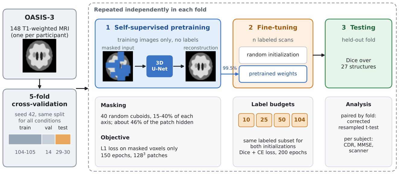
Figure 2.
Masked-volume pretraining on one patch (axial slice through the patch center). Left: original. Middle: input to the network, with masked voxels shown in blue (46 % of the patch). Right: output of the pretrained network, with visible voxels copied from the input. The patch comes from a test subject of the fold, which was not used for pretraining.
Figure 2.
Masked-volume pretraining on one patch (axial slice through the patch center). Left: original. Middle: input to the network, with masked voxels shown in blue (46 % of the patch). Right: output of the pretrained network, with visible voxels copied from the input. The patch comes from a test subject of the fold, which was not used for pretraining.
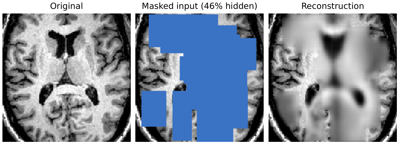
Figure 3.
Test Dice against the number of labeled training subjects, for random initialization and self-supervised pretraining. Points are means and error bars one standard deviation across five cross-validation folds; points are offset horizontally for legibility. The dashed line marks the randomly initialized model at .
Figure 3.
Test Dice against the number of labeled training subjects, for random initialization and self-supervised pretraining. Points are means and error bars one standard deviation across five cross-validation folds; points are offset horizontally for legibility. The dashed line marks the randomly initialized model at .
Figure 4.
Segmentation of a held-out test subject by models fine-tuned with 25 labeled scans. The subject has the median per-subject Dice gain among the 30 test subjects of its fold. Columns: T1-weighted image, FreeSurfer reference, randomly initialized model, pretrained model, and the voxel-wise change with pretraining (green: wrong with random initialization and correct with pretraining; red: the reverse). Dice is the mean over the 27 structures for this subject. Label colors follow the FreeSurfer lookup table; images are shown in neurological convention (the participant’s left on the left).
Figure 4.
Segmentation of a held-out test subject by models fine-tuned with 25 labeled scans. The subject has the median per-subject Dice gain among the 30 test subjects of its fold. Columns: T1-weighted image, FreeSurfer reference, randomly initialized model, pretrained model, and the voxel-wise change with pretraining (green: wrong with random initialization and correct with pretraining; red: the reverse). Dice is the mean over the 27 structures for this subject. Label colors follow the FreeSurfer lookup table; images are shown in neurological convention (the participant’s left on the left).
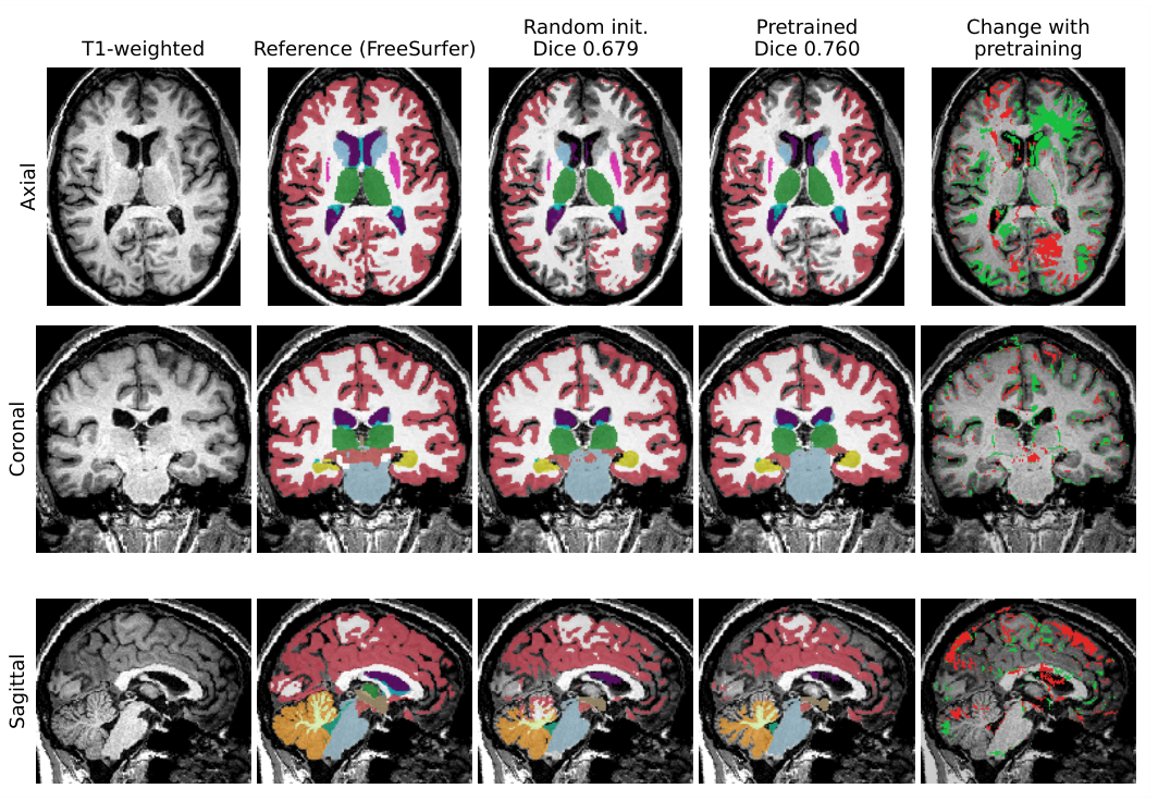
Figure 5.
(a) Per-structure Dice gain from self-supervised pretraining at (values of Table 4). (b) Gain against structure size, on a logarithmic axis. The association is weak and not significant. DC, diencephalon.
Figure 5.
(a) Per-structure Dice gain from self-supervised pretraining at (values of Table 4). (b) Gain against structure size, on a logarithmic axis. The association is weak and not significant. DC, diencephalon.
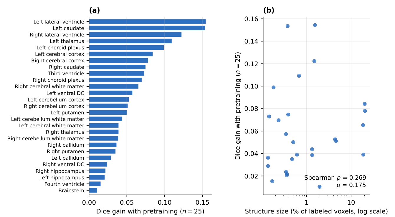

Table 1.
Cohort characteristics (, one imaging session per participant). Values are mean ± SD with range, or count (percentage). CDR, Clinical Dementia Rating [28]; MMSE, Mini-Mental State Examination [29].
| Characteristic | Value |
|---|---|
| Participants | 148 (one scan each) |
| Age at scan, years | (50.0–95.7) |
| Sex, female | 90 (60.8 %) |
| Sex, male | 58 (39.2 %) |
| Education, years | (8–22) |
| MMSE | (16–30) |
| CDR 0 (cognitively normal) | 112 (75.7 %) |
| CDR 0.5 (very mild) | 23 (15.5 %) |
| CDR 1 (mild) | 12 (8.1 %) |
| CDR 2 (moderate) | 1 (0.7 %) |
| Siemens TrioTim, 3 T | 102 (68.9 %) |
| Siemens Biograph mMR, 3 T | 37 (25.0 %) |
| Siemens MAGNETOM Vida, 3 T | 8 (5.4 %) |
| Siemens Sonata, 1.5 T | 1 (0.7 %) |
| Scan-to-clinic interval, days | median 92; 141/148 within 1 year |
Table 2.
Test Dice by labeled-data budget and initialization scheme. Mean ± SD over five cross-validation folds. The final column expresses pretrained performance as a percentage of the full-budget randomly initialized baseline (0.7997).
Table 2.
Test Dice by labeled-data budget and initialization scheme. Mean ± SD over five cross-validation folds. The final column expresses pretrained performance as a percentage of the full-budget randomly initialized baseline (0.7997).
| Random init. | SSL pretrained | % of | |
|---|---|---|---|
| n | Dice | Dice | baseline |
| 10 | 79.9 % | ||
| 25 | 95.7 % | ||
| 50 | 98.8 % | ||
| 104 | 101.8 % |
Table 3.
Paired comparison of self-supervised versus random initialization, matched by cross-validation fold (). CI is the 95 % confidence interval on the paired difference and CIcorr the interval under the corrected variance; is the ordinary paired t-test, the corrected resampled t-test accounting for the dependence between folds, the Wilcoxon signed-rank test, and d paired Cohen’s d.
Table 3.
Paired comparison of self-supervised versus random initialization, matched by cross-validation fold (). CI is the 95 % confidence interval on the paired difference and CIcorr the interval under the corrected variance; is the ordinary paired t-test, the corrected resampled t-test accounting for the dependence between folds, the Wilcoxon signed-rank test, and d paired Cohen’s d.
| n | Dice | 95 % CI | d | ||||
|---|---|---|---|---|---|---|---|
| 10 | 0.0092 | 0.0390 | 0.0625 | 2.11 | |||
| 25 | 0.0009 | 0.0050 | 0.0625 | 3.91 | |||
| 50 | 0.3550 | 0.5393 | 0.4375 | 0.47 | |||
| 104 | 0.0221 | 0.0802 | 0.0625 | 1.62 |
Table 4.
Per-structure Dice at labeled subjects, averaged over five folds, ordered by the gain attributable to pretraining. Size is the percentage of labeled voxels occupied by each structure, estimated from a 25-subject subsample. DC, diencephalon.
Table 4.
Per-structure Dice at labeled subjects, averaged over five folds, ordered by the gain attributable to pretraining. Size is the percentage of labeled voxels occupied by each structure, estimated from a 25-subject subsample. DC, diencephalon.
| Structure | SSL | Random | Gain | Size (%) |
|---|---|---|---|---|
| Left lateral ventricle | 0.8171 | 0.6627 | 0.1544 | 1.543 |
| Left caudate | 0.7285 | 0.5750 | 0.1535 | 0.374 |
| Right lateral ventricle | 0.8623 | 0.7401 | 0.1223 | 1.490 |
| Left thalamus | 0.8195 | 0.7102 | 0.1093 | 0.677 |
| Left choroid plexus | 0.4715 | 0.3725 | 0.0989 | 0.181 |
| Left cerebral cortex | 0.6298 | 0.5456 | 0.0842 | 20.164 |
| Right cerebral cortex | 0.6850 | 0.6070 | 0.0780 | 20.416 |
| Right caudate | 0.7932 | 0.7185 | 0.0747 | 0.387 |
| Third ventricle | 0.6232 | 0.5503 | 0.0730 | 0.144 |
| Right choroid plexus | 0.5517 | 0.4821 | 0.0696 | 0.235 |
| Right cerebral white matter | 0.7704 | 0.7051 | 0.0653 | 18.584 |
| Left ventral DC | 0.7534 | 0.6962 | 0.0573 | 0.343 |
| Left cerebellum cortex | 0.8503 | 0.7977 | 0.0526 | 4.371 |
| Right cerebellum cortex | 0.8670 | 0.8160 | 0.0511 | 4.571 |
| Left putamen | 0.8106 | 0.7605 | 0.0501 | 0.502 |
| Left cerebellum white matter | 0.8466 | 0.8028 | 0.0438 | 1.329 |
| Right thalamus | 0.8482 | 0.8092 | 0.0390 | 0.609 |
| Left cerebral white matter | 0.7608 | 0.7218 | 0.0390 | 18.808 |
| Right cerebellum white matter | 0.8544 | 0.8158 | 0.0386 | 1.336 |
| Right pallidum | 0.7565 | 0.7202 | 0.0363 | 0.136 |
| Right putamen | 0.8021 | 0.7671 | 0.0350 | 0.472 |
| Left pallidum | 0.6904 | 0.6615 | 0.0289 | 0.136 |
| Right ventral DC | 0.7816 | 0.7579 | 0.0237 | 0.346 |
| Right hippocampus | 0.8205 | 0.7988 | 0.0217 | 0.362 |
| Left hippocampus | 0.7939 | 0.7732 | 0.0206 | 0.359 |
| Fourth ventricle | 0.7742 | 0.7589 | 0.0153 | 0.169 |
| Brainstem | 0.8987 | 0.8884 | 0.0104 | 1.955 |
Table 5.
Subject-level analysis of segmentation accuracy (; one out-of-sample Dice score per participant). The two stratified rows separate scanner from disease, which are confounded in this cohort. is first group minus second. aMann–Whitney U; bKruskal–Wallis across the three scanner models with .
Table 5.
Subject-level analysis of segmentation accuracy (; one out-of-sample Dice score per participant). The two stratified rows separate scanner from disease, which are confounded in this cohort. is first group minus second. aMann–Whitney U; bKruskal–Wallis across the three scanner models with .
| Comparison | Groups (n) | Dice | p | |
|---|---|---|---|---|
| Disease, all scanners | CDR 0 (112) / CDR > 0 (36) | 0.8027 / 0.7856 | ||
| Scanner, all subjects | Biograph (37) / TrioTim (102) | 0.8261 / 0.7868 | ||
| Scanner, CDR 0 only | Biograph (33) / TrioTim (70) | 0.8273 / 0.7892 | ||
| Disease, TrioTim only | CDR 0 (70) / CDR > 0 (32) | 0.7892 / 0.7817 | ||
| Pretraining gain, severity | CDR 0 (112) / CDR > 0 (36) | / | ||
| Pretraining gain, scanner | Biograph / Vida / TrioTim | / / | ||
Disclaimer/Publisher’s Note: The statements, opinions and data contained in all publications are solely those of the individual author(s) and contributor(s) and not of MDPI and/or the editor(s). MDPI and/or the editor(s) disclaim responsibility for any injury to people or property resulting from any ideas, methods, instructions or products referred to in the content. |
© 2026 by the authors. Licensee MDPI, Basel, Switzerland. This article is an open access article distributed under the terms and conditions of the Creative Commons Attribution (CC BY) license (http://creativecommons.org/licenses/by/4.0/).
Copyright: This open access article is published under a Creative Commons CC BY 4.0 license, which permit the free download, distribution, and reuse, provided that the author and preprint are cited in any reuse.