

Submitted:
03 November 2026
Posted:
04 November 2026
You are already at the latest version
Abstract
Continuous monitoring of electromagnetic anomalies has gained critical relevance in earthquake precursory studies; however, reliable detection remains challenging due to non-stationary interference and noise. This study investigates the time frequency characteristics of EM signals at carrier frequencies of 3 kHz, 10 kHz, and 46 MHz over an 18-day window (±9 days around the seismic events). A combined framework consisting of Maximal Overlap Discrete Wavelet Transform (MODWT) for noise reduction followed by Continuous wavelet transform (CWT) was employed for anomaly detection for each frequency band. Hurst exponent was computed to check the persistent behavior of EM time series. Results portrays that the unusual, distinct, separable energy clusters were effectively captured by CWT scalograms in 3 kHz EM signals prior to the seismic events and are interpreted as possible seismogenic emanations. Unlike the 3 kHz signal, the 10 kHz and 46 MHz signals show either diffused or homogeneous distribution indicating no detectable earthquake related components. Results validate that EM precursors are strongly frequency dependent, with optimal detectability in the lower very low frequency region (∼3 kHz and ~10 kHz), whilst higher-frequency (46 MHz) region mostly show less detectable anomalies may be due to greater attenuation and external noise influences. Hurst exponent portrays that 46 MHz signal shows strong persistence throughout as compared to 3 kHz and 10 kHz signals as these low frequency signals are more susceptible to noise. This study highlights the importance of frequency selection and advance signal processing techniques in seismic related anomaly detection.
Keywords:
anomaly detection
; electromagnetic disturbances
; kHz
; MHz
; continuous wavelet transform
; hurst exponent
1. Introduction
Anomaly detection in electromagnetic (EM) signals has gained significant attention due to its wide-ranging applications across scientific fields including environmental monitoring [1], industrial diagnostics [2], telecommunications [3], earthquake forecasting [4], and astronomy [5]. The frequency ranges of EM signals studied in the literature range from ultra-low frequencies (ULF) [0.001 Hz - 1 Hz] [6,7], low frequencies (LF) (1 kHz - 10 kHz) [8,9], high frequencies (HF) (40 MHz - 60 MHz) [10,11] very high frequencies (VHF) [up to 300 MHz] [12].
Anomalies in EM signals signify sudden shifts in amplitude, frequency, or phase which may be caused by equipment faults (e.g., power cable partial discharge), structural reflections in radar echoes, or environmental changes in wireless systems [13]. These transient anomalies are characterized by their short duration and are particularly challenging to capture using traditional Fourier-based methods, which rely on the assumption of signal stationarity over time. As a result, conventional approaches often fail to detect these brief but significant events, which can indicate equipment malfunction, interference, or other rare occurrences [14].
The Wavelet Transform (WT) has emerged as a powerful and widely utilized tool in the signal analysis and processing studies, particularly for analyzing non-linear and non-stationary signals in anomaly detection applications [15]. The WT is a mathematical approach that is frequently utilized in the time frequency domain of signal analysis. It also enables effective noise reduction while preserving the essential characteristics of the signal [16]. Denoising can be defined as a signal processing technique used to remove the noise from the input signal while maintaining the important features of the wanted signal [17]. As most signals in the real world are non-stationary, so, denoising and decomposition of those signals is necessary to study the important features associated with the signal. Some modern sophisticated signal processing and decomposition techniques includes Empirical Mode Decomposition (EMD) [18], Variational Mode Decomposition (VMD) [19], and Discrete Wavelet Transform (DWT) [20] have been employed for the decomposition of input signal. Notably, a recent work has successfully applied MODWT to electrocardiogram (ECG) signals [21], achieving maximum sensitivity for both noisy and denoised data in pathological examinations.
In Wavelet based techniques, the continuous wavelet transform (CWT) is optimal for analyzing non-stationary signals due to its superior time-frequency resolution. The WT is a signal decomposition technique that is non-adaptive but it multi-resolution analysis (MRA) of time and frequency domains [22]. Rasheed et al. [15] demonstrated the effectiveness of CWT for the detection of anomalies in radon, thoron and meteorological time series data, establishing a clear relationship with seismic events occurred during their study period. Results demonstrate that CWT performs better in detecting anomalies in radon, thoron and meteorological time series data.
The Hurst exponent is frequently used in fractal analysis to evaluate the long term memory and fractality in time series data. Hurst exponent is done by measuring the rescaled range analysis of time series. The Hurst exponent can classify the given time series in terms of random, persistent and anti-persistent nature [23]. Hayakawa et al. [24] employed the Hurst exponent analysis on ultra-low frequency components of geomagnetic field signals. Their results portrays that the Hurst exponent shows persistent behavior and is related to random field variations that increases as earthquake energy increases.
This research investigates the continuous wavelet transform (CWT) scalograms for the detection of anomalies in continuous EM time series data. The maximal overlap discrete wavelet transform (MODWT) was employed on the EM time series to separate noise and de-noised signals. After decomposition, the denoised EM signals have been reconstructed, and sym4 wavelet based CWT scalograms of the reconstructed de-noised signals are computed to identify anomalies in EM signals. Furthermore, Hurst exponent is calculated to check the fractal behavior of EM time series data.
2. Materials and Methods
2.1. Area of Study
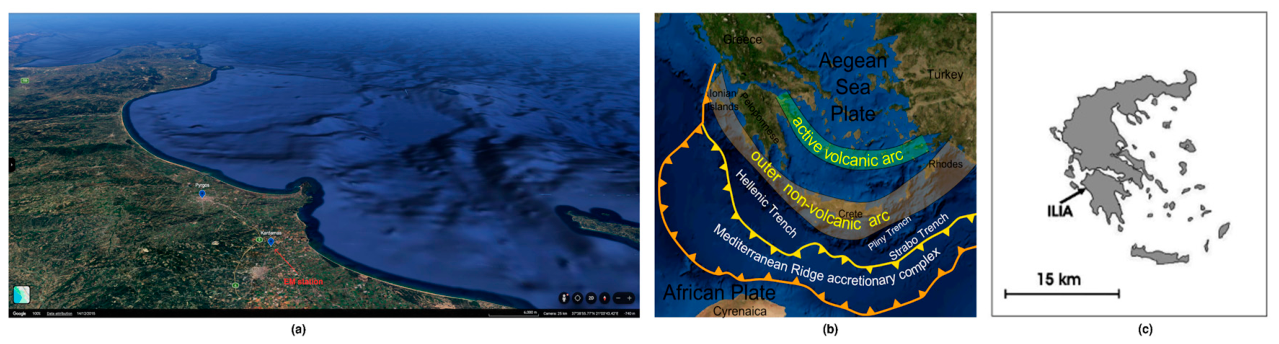
This research was conducted at Ilia, located in southwestern Greece, within a tectonically complex landscape located near the boundary between the African and Eurasian plates. The region hosts electromagnetic monitoring station at Kardamas (37°46″N 21°20′E (Figure. 1). The geology of the study site comprises of Mesozoic-early Cenozoic carbonate rocks that were originally placed on a number of zones (pre-Apulian and Gavrovo) and basins (Ionian and Pindos). These carbonate formation extend along thrust faults that strike north-south, dip east and transition upward and westward into subordinate flysch deposits [25]. This geological setting males the region highly suitable for observing both natural EM variations and potential seismo-electromagnetic phenomena.
The monitoring station is equipped with magnetic loop antennas, and vertical electric field antennae, enabling synchronized observations across the low frequency (LF) from 1 to 10 kHz, and high frequencies (HF) from 40 to 60 MHz bands. This configuration provides comprehensive EM datasets suitable for detailed research and analysis [26].
Figure 1.
The study area with related information. (a) Map from GoogleMaps showing Kardamas Village, and Pyrgos city, which is the capital of Ilia and the EM station in Kardamas (in red). The trench in the opposite direction of the whole area near the EM station, is shown as differentiations in the sea depth, which are characteristically presented in this view of Google maps; (b) The tectonic background of the study area showing the seismic plates surrounding south-west Peloponnese and Crete, the volcanic arcs, the surrounding trenches in yellow and the far trenches in orange [27]; (c) A simple map of Greece showing Peloponnese and Ilie Prefecture as a black arrow.
Figure 1.
The study area with related information. (a) Map from GoogleMaps showing Kardamas Village, and Pyrgos city, which is the capital of Ilia and the EM station in Kardamas (in red). The trench in the opposite direction of the whole area near the EM station, is shown as differentiations in the sea depth, which are characteristically presented in this view of Google maps; (b) The tectonic background of the study area showing the seismic plates surrounding south-west Peloponnese and Crete, the volcanic arcs, the surrounding trenches in yellow and the far trenches in orange [27]; (c) A simple map of Greece showing Peloponnese and Ilie Prefecture as a black arrow.
2.2. Instrumentation
The electromagnetic (EM) disturbances are continuously monitored by the Kardamas EM station at a rate of 1 through (a) Circular magnetic field antennas synchronized at 3 and at 10 . Two orientations are installed. One at the east-west (EW) orientation and the other at the north-south (NS) orientation; (b) Electric dipole wavelength/4 loop antennas synchronised at 41 MHz and 46 both at the east-west orientation; (c) Campbell CR-10 data-logger with a 2 h buffer; (d) Telemetry equipment continuously sending the measurements to a personal computer.
2.3. Mathematical Methodology
2.3.1. Maximal Overlap Discrete Wavelet Transform (MODWT)
The maximal overlap discrete wavelet transform is the modified version of the discrete wavelet transform (DWT) specifically designed for time series applications. The MODWT is more beneficial than DWT because of its ability to provide high-quality information with a focus on wavelet and scaling coefficients. Unlike DWT which discards the results of down sampling, MODWT retains these results of down sampling at every decomposition level, thereby preserve more signal information. This approach uses low-pass and high-pass filters to separate the frequency components of input (sound) signals into distinct scales [28].
DWT represents one of the most important signal decomposition technique employing linear transformation for mapping the time series, to the vector with wavelet coefficients of length in the wavelet domain. Let be the mother wavelet, and the translation and dilation operations using DWT can be expressed as [29]
where are the orthonormal basis of the wavelet function. The input signal , can be expressed as
where represents the wavelet coefficient of signal . The advantages of MODWT over DWT is that it could be applied to any sample size and is translational invariant, overcomes the limitation of DWT on sample size that should be a multiple of and its sensitivity to circular shifts caused by the down sampling strategy at the expense of orthogonality [30].
Unlike DWT, MODWT generates shift-invariant, zero-phase wavelet and scaling coefficients, meaning that features in the original signal such as sudden spikes align precisely with corresponding features in the transform. Additionally, MODWT does not require dyadic (power-of-two) sample lengths [31]. Outlining the scaling and wavelet filters and respectively where is the width of the wavelet. he wavelet and scaling coefficients are expressed as [32]
and
The MODWT can be utilized to perform multi-resolution analysis (MRA) of the signal. This MRA differs from the standard DWT in which each detail of the signal will be circularly shifted by a proportional amount when the time series undergoes any circular shift. These details are associated with to zero phase filters, making MRA both reliable and easier to interpret in terms of meaningful signal features [33].
2.3.2. The Continuous Wavelet Transform (CWT)
The Continuous Wavelet Transform CWT of a signal can be represented as the convolution of the input signal multiplied with the scaled and shifted versions of a wavelet function over the time. The CWT is defined as [34]
and can be calculated as
The parameters and are used to scale and shift the wavelets respectively. represents the complex conjugation and the normalizing factor guarantees that the energy remains constant across all scale levels. The CWT projects a signal into two dimensional time-scale phase plane by presenting it with a wavelet function. Contrary to the short-time Fourier transform (STFT), CWT can deal with the discrepancies between time and frequency resolutions due to its configurable time-frequency window. After shifting a function known as the “mother wavelet,” an inner product between the function and the signal which will be processed at various scales is formed [35].
2.3.3. The Hurst Exponent (H)
The Hurst exponent is a popular approach in time series analysis (TSA) to measure the long term memory and irregularities existing in a time series. As it is robust with limited assumptions about underlying system, it has comprehensive applications for TSA. The Hurst exponent ranges between 0 and 1. A time series can be categorized into three groups on the basis of Hurst exponent such as H=0.5 shows a random series, H<0.5 portrays an anti-persistent series while H>0.5 indicates the persistent time series [36]. The Hurst exponent is calculated using the rescaled range (R/S) analysis such as
where (R/S) is the rescaled range, ‘n’ represents the number of samples.
3. Results and Discussion
Figure 2 through 7 portrays the original 3 kHz, 10 kHz and 46 MHz EM time series data signals recorded for 18 day time window, 9 days before and after the seismic event occurred during the study. Table 1 demonstrate the seismic data recorded during the study period whilst Table 2 through 7 presents the descriptive statistics (mean, median, standard deviation, median, maximum and minimum) values recorded for 3 kHz, 10 kHz and 46 MHz EM time series data signals.
Figure 2.
Original 3 kHz, 10 kHz, and 46 MHz signal ±9 days before and after 6 February, 2024 earthquake.
Figure 2.
Original 3 kHz, 10 kHz, and 46 MHz signal ±9 days before and after 6 February, 2024 earthquake.
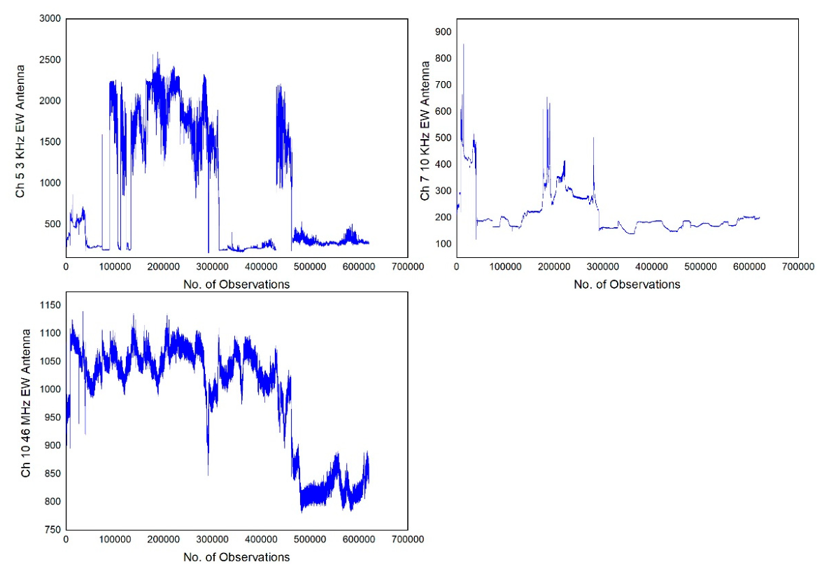
Figure 3.
Original 3 kHz, 10 kHz, and 46 MHz signal ±9 days before and after 29 March, 2024 earthquake.
Figure 3.
Original 3 kHz, 10 kHz, and 46 MHz signal ±9 days before and after 29 March, 2024 earthquake.
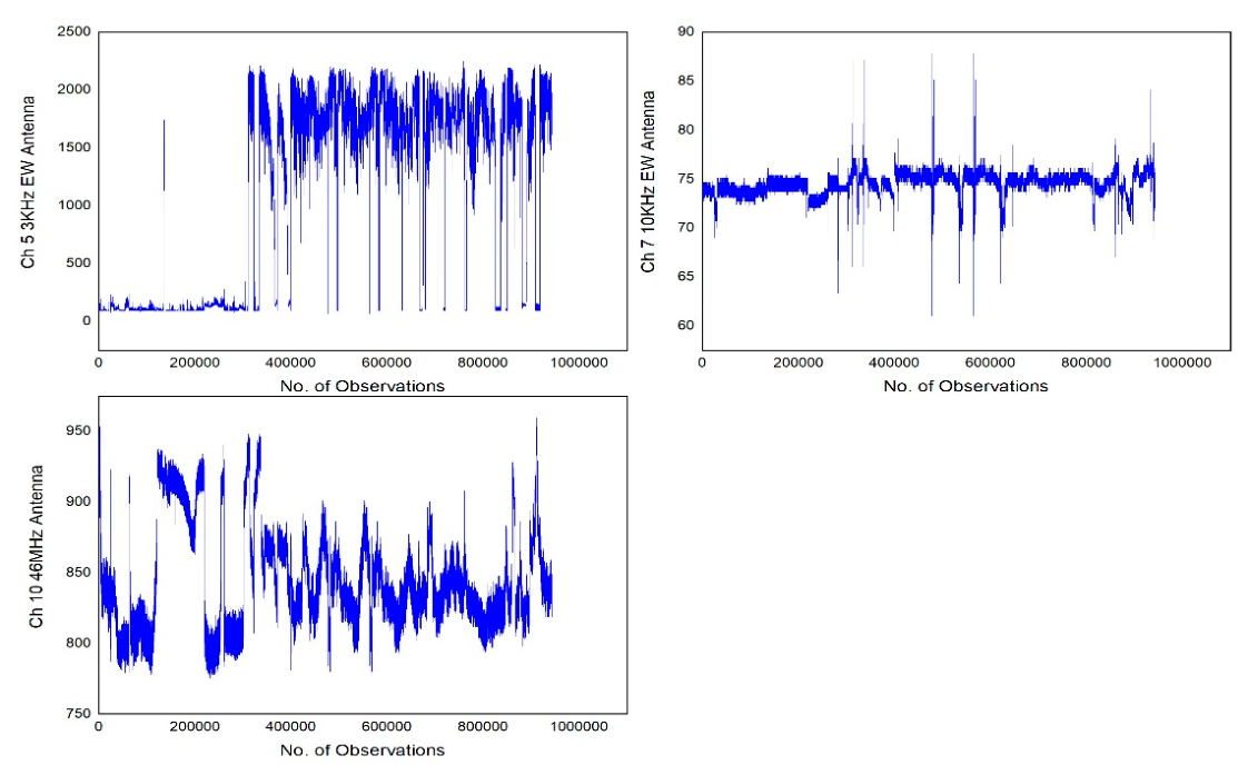
Figure 4.
Original 3 kHz, 10 kHz, and 46 MHz signal ±9 days before and after 6 and 7 July, 2024 earthquake.
Figure 4.
Original 3 kHz, 10 kHz, and 46 MHz signal ±9 days before and after 6 and 7 July, 2024 earthquake.
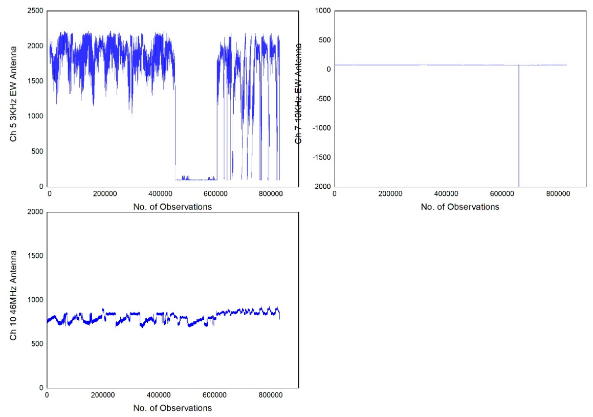
Figure 5.
Original 3 kHz, 10 kHz, and 46 MHz signal ±9 days before and after 14 July. 2024 earthquake.
Figure 5.
Original 3 kHz, 10 kHz, and 46 MHz signal ±9 days before and after 14 July. 2024 earthquake.
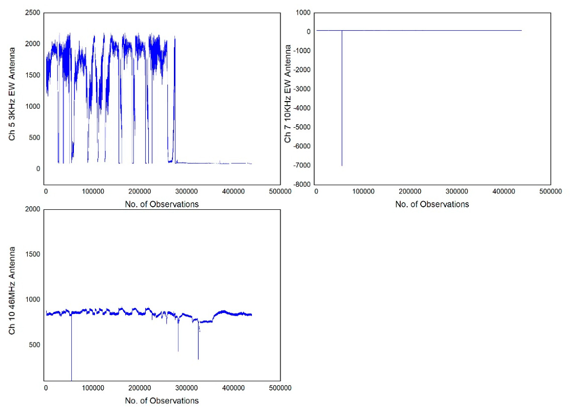
Figure 6.
Original 3 kHz, 10 kHz, and 46 MHz signal ±9 days before and after 28 September, 2024 earthquake.
Figure 6.
Original 3 kHz, 10 kHz, and 46 MHz signal ±9 days before and after 28 September, 2024 earthquake.
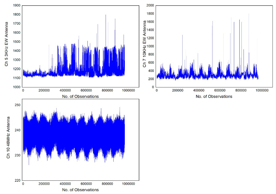
Figure 7.
Original 3 kHz, 10 kHz, and 46 MHz signal ±9 days before and after 14 July. 2024 earthquake.
Figure 7.
Original 3 kHz, 10 kHz, and 46 MHz signal ±9 days before and after 14 July. 2024 earthquake.
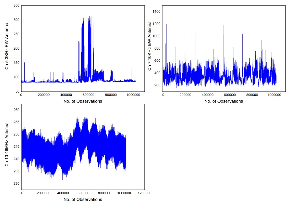

Table 1.
Date, Magnitude, Latitude, Longitude and depth information of Seismic data for the year 2024.
Table 1.
Date, Magnitude, Latitude, Longitude and depth information of Seismic data for the year 2024.
| Date | Magnitude (ML) | Latitude (0) | Longitude (0) | Depth (km) |
| 06-02-2024 | 3.9 | 37.65 | 20.54 | 17 |
| 29-03-2024 | 4.1 | 37.19 | 21.17 | 27 |
| 29-03-2024 | 5.8 | 37.20 | 21.19 | 29 |
| 29-03-2024 | 3.5 | 37.27 | 21.25 | 24 |
| 29-03-2024 | 3.6 | 37.18 | 21.19 | 32 |
| 29-03-2024 | 3.5 | 37.18 | 21.19 | 29 |
| 06-07-2024 | 4.9 | 37.84 | 21.18 | 11 |
| 07-07-2024 | 4.7 | 37.82 | 21.18 | 6 |
| 14-07-2024 | 3.5 | 37.82 | 21.15 | 17 |
| 28-09-2024 | 4.4 | 37.31 | 21.25 | 18 |
| 27-11-2024 | 3.5 | 37.82 | 21.14 | 17 |
Table 2.
Mean, Median, Standard deviation, maximum and minimum values of EM signals before and after 6 February, 2024 earthquake.
Table 2.
Mean, Median, Standard deviation, maximum and minimum values of EM signals before and after 6 February, 2024 earthquake.
| No of observations | 3 kHz signal | 10 kHz signal | 46 MHz signal |
| Mean | 862.6 | 216.8 | 986.5 |
| Median | 322.5 | 187 | 1028 |
| Standard deviation | 767 | 76.9 | 98.9 |
| Maximum | 2606 | 855 | 1140 |
| Minimum | 155.8 | 118.7 | 780 |
Table 3.
Mean, Median, Standard deviation, maximum and minimum values of EM signals before and after 29 March, 2024 earthquake.
Table 3.
Mean, Median, Standard deviation, maximum and minimum values of EM signals before and after 29 March, 2024 earthquake.
| No of observations | 3 kHz signal | 10 kHz signal | 46 MHz signal |
| Mean | 1092.6 | 74.5 | 845.5 |
| Median | 1556 | 74.5 | 836 |
| Standard deviation | 836.6 | 1.1 | 35.8 |
| Maximum | 2247 | 87.8 | 960 |
| Minimum | 69.4 | 61 | 776 |
Table 4.
Mean, Median, Standard deviation, maximum and minimum values of EM signals before and after 6 and 7 July, 2024 earthquake.
Table 4.
Mean, Median, Standard deviation, maximum and minimum values of EM signals before and after 6 and 7 July, 2024 earthquake.
| No of observations | 3 kHz signal | 10 kHz signal | 46 MHz signal |
| Mean | 1462.1 | 79.7 | 806.2 |
| Median | 1807 | 79.7 | 804 |
| Standard deviation | 732 | 7.81 | 52.1 |
| Maximum | 2218 | 82.4 | 929 |
| Minimum | 91.8 | -6999 | -6999 |
Table 5.
Mean, Median, Standard deviation, maximum and minimum values of EM signals before and after 14 July, 2024 earthquake.
Table 5.
Mean, Median, Standard deviation, maximum and minimum values of EM signals before and after 14 July, 2024 earthquake.
| No of observations | 3 kHz signal | 10 kHz signal | 46 MHz signal |
| Mean | 987.5 | 79.4 | 842.4 |
| Median | 1150 | 79.7 | 848 |
| Standard deviation | 839.2 | 10.7 | 40.7 |
| Maximum | 2185 | 81.7 | 929 |
| Minimum | 88.4 | -6999 | -6999 |
Table 6.
Mean, Median, Standard deviation, maximum and minimum values of EM signals before and after 28 September, 2024 earthquake.
Table 6.
Mean, Median, Standard deviation, maximum and minimum values of EM signals before and after 28 September, 2024 earthquake.
| No of observations | 3 kHz signal | 10 kHz signal | 46 MHz signal |
| Mean | 1165.3 | 285.6 | 237.9 |
| Median | 1139.1 | 275.9 | 238 |
| Standard deviation | 64.6 | 53.5 | 2.44 |
| Maximum | 1800 | 1800 | 249.2 |
| Minimum | 1098.4 | 158.5 | 226.2 |
Table 7.
Mean, Median, Standard deviation, maximum and minimum values of EM signals before and after 27 November, 2024 earthquake.
Table 7.
Mean, Median, Standard deviation, maximum and minimum values of EM signals before and after 27 November, 2024 earthquake.
| No of observations | 3 kHz signal | 10 kHz signal | 46 MHz signal |
| Mean | 90.5 | 344.6 | 244.4 |
| Median | 84.3 | 331.1 | 244.3 |
| Standard deviation | 22.2 | 86.8 | 3.3 |
| Maximum | 314.5 | 1339 | 257.9 |
| Minimum | 79.6 | 150.4 | 230.6 |
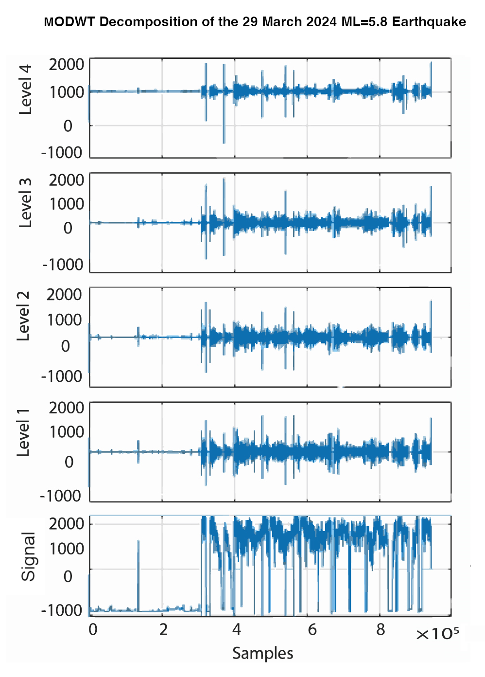
MODWT decomposition of the EM signal was performed using sym4 wavelets (see Figure 8 through 13). For the MODWT decomposition, time is plotted on X-axis and the Y-axis portrays the amplitude of the decomposed signal. The level of decomposition for 3 kHz, 10 kHz and 46 MHz signal is taken as 4. The “level” of decomposition refers to the degree with which we want to denoise or decompose the signal
If the decomposition level is increased, signal decomposes at high level but the drawback to high level decomposition is that it eliminates the meaningful features associated with the signal therefore we must select the intermediate level of decomposition to preserve all of the meaningful features while extracting the relevant information. The approximation of the signal refers to the lowest frequency-band scale, while the details, which are in rising octave frequency bands, are the other scales.
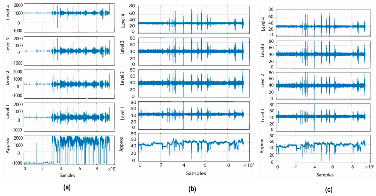
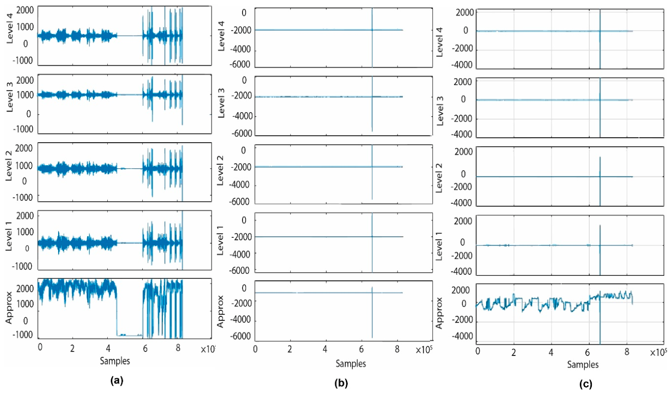
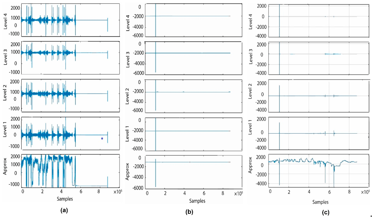
Figure 8 through 13 shows the MODWT decomposition of 3 kHz, 10 kHz and 46 MHz EM signal for each seismic event data. Level 1 portrays the highest frequency details (smallest scale), levels 2 to 4 represent progressively lower frequency details of the signal. Notable spikes are visible in level 1 and level 2 representing the high energy bursts or transients in the higher-frequency range that could be due to the anomalies, sudden EM events, or noise burst. Levels 3 and 4 also indicate original burst is still visible although a few random spikes are also observed. Intermittent disruptions in the electromagnetic transmission may be represented by these mid-band anomalies. The total amplitude trend portrayed by the approximation shows a significant peak at the beginning followed by decay. Localized anomalies in both mid and low-frequency broadband disruption are observed, as initial bursts are observed throughout the decomposition and the subsequent spikes observed across all levels. Strong sharp spikes across all decomposition levels indicate a broadband transient event containing significant energy across high, mid, and low frequency components. At approximation level, there is a deep drop in a signal confirming the low-frequency content that is likely caused by a sudden, high-energy interference or EM burst. The presence of multiple peaks suggest broadband anomalies rather than narrowband noise. The approximation component proves particularly valuable for identifying low-frequency anomalies that may not show up in high-frequency detail levels.
Table 8.
Results of Hurst exponent employed on EM signals ±9 days before the seismic events.
| No of observations | 3 kHz signal | 10 kHz signal | 46 MHz signal |
| 6 February 2026 | 0.53 | 0.42 | 0.75 |
| 29 March 2026 | 0.28 | 0.55 | 0.77 |
| 6 and 7 July 2026 | 0.66 | 0.38 | 0.73 |
| 14 July 2026 | 0.19 | 0.79 | 0.73 |
| 28 September 2026 | 0.82 | 0.79 | 0.98 |
| 27 November 2026 | 0.91 | 0.78 | 0.95 |
To identify anomalies in the 3 kHz, 10 kHz and 46 MHz EM signals, sym4 based CWT scalograms were used. The scalograms of a signal are the absolute value of CWT, a map showing relationship between time and frequency content of a signal where time and frequency are plotted on x-axis and y-axis respectively. Figure 14 through 19 portrays the CWT scalograms employed sym4 decomposed 3 kHz, 10 kHz and 46 MHz EM signals ±9 days before and after the seismic events occurred during the study period. Red plot (see Figure 14 to 19) represents the time domain representation of the input signal after being reconstructed from a level-4 MODWT decomposition and then examined by using CWT scalograms.
Figure 14 shows CWT scalogram of 3 kHz, 10 kHz and 46 MHz EM signal ±9 days before and after the seismic event of magnitude (ML 3.9) occurred on 6th of February 2024.
Figure 8.
MODWT decomposition of EM signals ±9 days before and after 6 February earthquake; (a) MODWT decomposition of 3 kHz signal; (b) MODWT decomposition of 10 kHz signal; (c) MODWT decomposition of 46 MHz signal.
Figure 8.
MODWT decomposition of EM signals ±9 days before and after 6 February earthquake; (a) MODWT decomposition of 3 kHz signal; (b) MODWT decomposition of 10 kHz signal; (c) MODWT decomposition of 46 MHz signal.
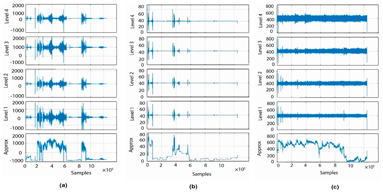
Figure 9.
MODWT decomposition of EM signals ±9 days before and after 29 March earthquake; (a) MODWT decomposition of 3 kHz signal; (b) MODWT decomposition of 10 kHz signal; (c) MODWT decomposition of 46 MHz signal.
Figure 9.
MODWT decomposition of EM signals ±9 days before and after 29 March earthquake; (a) MODWT decomposition of 3 kHz signal; (b) MODWT decomposition of 10 kHz signal; (c) MODWT decomposition of 46 MHz signal.
The sudden bright colors (red/yellow) were observed in 3 kHz and 46 MHz signals indicating the high spectral power, high-frequency bursts and persistent high-energy bands before and after the occurrence of seismic event confirming the presence of anomaly in the EM signal. In EM interference analysis, this could be due to short impulsive noise burst or the environmental EM transient. Some portion of scalogram is dark blue, meaning low energy and no significant transient features after the initial bursts. For 10 kHz signal, the strong activity suggests there was an EM disturbance or event right at the beginning of the signal.
Figure 10.
MODWT decomposition of EM signals ±9 days before and after 6 and 7 July earthquake; (a) MODWT decomposition of 3 kHz signal; (b) MODWT decomposition of 10 kHz signal; (c) MODWT decomposition of 46 MHz signal.
Figure 10.
MODWT decomposition of EM signals ±9 days before and after 6 and 7 July earthquake; (a) MODWT decomposition of 3 kHz signal; (b) MODWT decomposition of 10 kHz signal; (c) MODWT decomposition of 46 MHz signal.
The signal then stabilizes, with only low-amplitude fluctuations present afterward. CWT scalogram of MODWT-decomposed 3 kHz signal shows no significant transient features initially but as the signal proceeds the unusual patterns were captured from mid till end of the signal indicating the presence of some high-energy regions with bright colors signifying strong signal activity. This could correspond to transient events (spikes, bursts) or oscillations of signal at certain frequencies. Some low-energy regions (dark colored areas) were observed where the signal correlates weakly with the wavelet, indicating silence or noise.
Figure 15 represents CWT scalogram of 3 kHz, 10 kHz and 46 MHz EM signal ±9 days before and after the seismic events. Five seismic events of magnitude (ML=4.1, ML=5.8, ML=3.5, ML=3.6 and ML=3.5) were recorded on 29th of March 2024 at different time spans. CWT scalogram of MODWT-decomposed 3 kHz signal shows no significant transient features initially but as the signal proceeds the unusual patterns were captured from mid till end of the signal indicating the presence of some high-energy regions with bright colors signifying strong signal activity. This could correspond to transient events (spikes, bursts) or oscillations of signal at certain frequencies. Some low-energy regions (dark colored areas) were observed where the signal correlates weakly with the wavelet, indicating silence or noise. In contrast with 3 kHz signal, no visible spectral patterns were observed for 10 kHz and 46 MHz signals. The lack of anomalous patterns for 10 kHz and 46 MHz may be due to the fact that these signals may experience significant attenuation during the propagation through crustal rocks or deviation from heterogeneities in the seismic zone.
Figure 16 represents CWT scalogram of 3 kHz, 10 kHz and 46 MHz EM signal ±9 days before and after the seismic events of magnitude (ML=4.9 and ML=4.7) occurred on 6th and 7th of July 2024. The CWT scalogram shows the anomalous patterns throughout the signal indicating the presence of transient energy bands within the signal. Transient electromagnetic bursts are represented by distinct high energy characteristics that are mostly focused in the pre-seismic event interval in the CWT scalogram for the 3 kHz signal. These spectral bursts, also known as anomalous emanations, are characteristics of non-stationary processes and may be connected to stress buildup and micro-fracturing that took place in the Earth’s crust. Both the signal’s frequency and energy rise as the seismic event gets closer, indicating increased geodynamic activity. No specific patterns were found for 10 kHz and 46 MHz signals indicating homogeneity of scalogram that may be due to low energy backgrounds, stationary external noise or radio frequency (RF) interferences.
Figure 11.
MODWT decomposition of EM signals ±9 days before and after 14 July earthquake; (a) MODWT decomposition of 3 kHz signal; (b) MODWT decomposition of 10 kHz signal; (c) MODWT decomposition of 46 MHz signal.
Figure 11.
MODWT decomposition of EM signals ±9 days before and after 14 July earthquake; (a) MODWT decomposition of 3 kHz signal; (b) MODWT decomposition of 10 kHz signal; (c) MODWT decomposition of 46 MHz signal.
In contrast with 3 kHz signal, no visible spectral patterns were observed for 10 kHz and 46 MHz signals. The lack of anomalous patterns for 10 kHz and 46 MHz may be due to the fact that these signals may experience significant attenuation during the propagation through crustal rocks or deviation from heterogeneities in the seismic zone. Figure 17 represents CWT scalogram of 3 kHz, 10 kHz and 46 MHz EM signal ±9 days before and after the seismic events of magnitude (ML=3.5) occurred on 14th of July 2024. The CWT scalogram for 3 kHz signal shows separate high energy features concentrated mainly in the pre-seismic event interval, representing transient EM bursts. These spectral bursts are features of non-stationary processes and are referred as anomalous emanations that may be linked with stress accumulation and micro-fracturing occurred within the Earth crust. As the seismic event approaches, the frequency as well as the energy of the signal increase, signifying greater geodynamic activity. However, after the seismic event low-energy patterns are observed in the scalogram, indicating the return to background conditions following stress release. 3 kHz CWT scalogram offers convincing evidence that sym4-based time-frequency (TF) analysis can effectively identify seismic precursors, with the detected patterns showcasing the possible tool for detecting the characteristic seismogenic signals from background EM emanation.
Figure 12.
MODWT decomposition of EM signals ±9 days before and after 28 September earthquake; (a) MODWT decomposition of 3 kHz signal; (b) MODWT decomposition of 10 kHz signal; (c) MODWT decomposition of 46 MHz signal.
Figure 12.
MODWT decomposition of EM signals ±9 days before and after 28 September earthquake; (a) MODWT decomposition of 3 kHz signal; (b) MODWT decomposition of 10 kHz signal; (c) MODWT decomposition of 46 MHz signal.
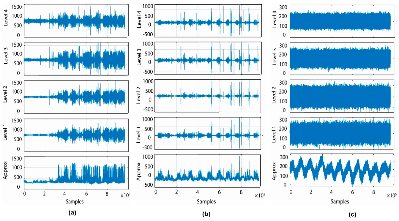
Figure 13.
MODWT decomposition of EM signals ±9 days before and after 27 November earthquake; (a) MODWT decomposition of 3 kHz signal; (b) MODWT decomposition of 10 kHz signal; (c) MODWT decomposition of 46 MHz signal.
Figure 13.
MODWT decomposition of EM signals ±9 days before and after 27 November earthquake; (a) MODWT decomposition of 3 kHz signal; (b) MODWT decomposition of 10 kHz signal; (c) MODWT decomposition of 46 MHz signal.
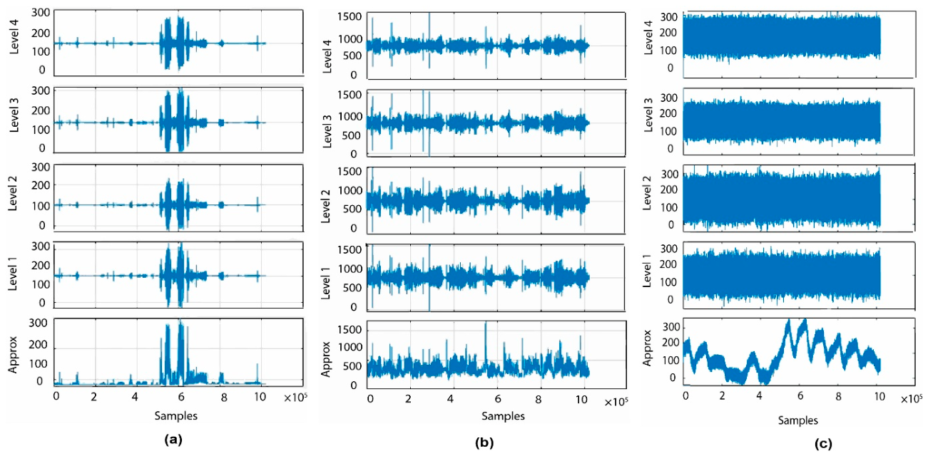
Figure 17 represents CWT scalogram of 3 kHz, 10 kHz and 46 MHz EM signal ±9 days before and after the seismic events of magnitude (ML=3.5) occurred on 14th of July 2024. The CWT scalogram for 3 kHz signal shows separate high energy features concentrated mainly in the pre-seismic event interval, representing transient EM bursts. These spectral bursts are features of non-stationary processes and are referred as anomalous emanations that may be linked with stress accumulation and micro-fracturing occurred within the Earth crust. As the seismic event approaches, the frequency as well as the energy of the signal increase, signifying greater geodynamic activity. However, after the seismic event low-energy patterns are observed in the scalogram, indicating the return to background conditions following stress release. 3 kHz CWT scalogram offers convincing evidence that sym4-based time-frequency (TF) analysis can effectively identify seismic precursors, with the detected patterns showcasing the possible tool for detecting the characteristic seismogenic signals from background EM emanation. In contrast to the 3 kHz signal results, 10 kHz shows stable behavior throughout with only single, transient impulsive peak observed at the start of the signal. This peak is clearly noticeable in both the MODWT-decomposed signal and the corresponding CWT scalogram indicating the lack of pre-seismic anomalies. However, apart from this transient event, the scalogram is predominantly characterized by dark blue regions, showing lack of persistent EM activity. For 46 MHz signal, the CWT scalogram is mostly characterized by dark blue regions indicating low-energy areas across the signal. Two unusual vertical colored lines were observed, corresponding to the sudden drops in the time series. These spectral features exhibit transient, broadband disturbances but lack of temporal clustering that may occur due to the external factors that influence the EM emissions.
Figure 18 portrays CWT scalogram of 3 kHz, 10 kHz and 46 MHz EM signal ±9 days before and after the seismic events of magnitude (ML=4.4) occurred on 28th of September 2024. CWT scalogram of 3 kHz and 10 kHz signal shows non-uniform distribution of energy where high-energy regions represented by warmer colors (red/yellow) appear irregularly throughout the signal. This anomalous cluster starts mainly from halfway signifying that the definite frequency variations around the 3 kHz carrier are especially excited during the occurrence of seismic event and possibly post-seismic phases. The CWT scalogram indicates that the low energy levels indicated by blue to green regions dominate whilst the anomalous high-energy regions represent transient enhancements above this baseline. These transient anomalies appearing as discrete incidents may be due to irregular micro-fracturing, or fluid flow dynamics within the seismogenic region. In contrast to the 3 kHz and 10 kHz signal, the scalogram of 46 MHz does not exhibit any warm color indicating the lack of transient energy patterns that would specify seismogenic EM emanations. The consistency of the scalogram demonstrates that the MODWT decomposed 46 MHz signal is influenced by external noise, meteorological parameters, or anthropogenic radio frequency (RF) interferences.
Figure 19 portrays CWT scalogram of 3 kHz, 10 kHz and 46 MHz EM signal ±9 days before and after the seismic events of magnitude (ML=3.5) occurred on 27th of November, 2024. CWT scalogram of 3 kHz signal detects the presence of anomalies that may occur due to earthquake-related EM precursors. The CWT shows significant variations in spectral energy throughout the signal. The scalogram shows non-uniform energy distributions with localized high-frequency clusters represented by warmer colors. The background energy levels represented by blue color dominate throughout indicating the presence of background noise whilst anomalous transient energy bands were observed indicating the emanation of EM energy from the seismogenic region. Unlike the 3 kHz CWT scalogram, the 10 kHz scalogram shows broader, more diffuse regions that lack sharp temporal boundaries. This pattern may show the occurrence of persistent background EM activity or interferences that may occur due to navigation systems, industrial noise, or meteorological parameters that influence the 10 kHz band rather than genuine seismogenic emanations. The lack of anomalous patterns for 46 MHz was observed that may occur due to significant attenuation during the propagation through crustal rocks or deviation from heterogeneities in the seismic zone.
Table 8 demonstrates the results of Hurst exponent computed for the EM signals ±9 days before and after the seismic events occurred during the study period. Hurst exponent were computed to investigate the temporal dynamics and long range dependency of EM signals at carrier frequencies of 3 kHz, 10 kHz and 46 MHz. The results reveal the frequency dependent response and temporal varying response in EM signals. The 46 MHz signal shows persistent behavior (H>0.5) throughout the study indicating the directional trend in the signal. Conversely, the lower frequency bands (3 kHz and 10 kHz) displayed significant non-stationarity. Both signals initially shows anti persistent behavior (H<0.5) but later on after 14 July the lower frequency bands transitioned into strongly persistent behavior (H>0.75). This increase in the Hurst exponent suggests a systematic environmental or source driven change rather than random noise.
Figure 14.
CWT scalograms of MODWT-decomposed signal for 6 February earthquake: (a) CWT scalogram of 3 kHz MODWT decomposed signal; (b) CWT scalo gram of 10 kHz MODWT decomposed signal; (c) CWT scalogram of 46 MHz MODWT decomposed signal.
Figure 14.
CWT scalograms of MODWT-decomposed signal for 6 February earthquake: (a) CWT scalogram of 3 kHz MODWT decomposed signal; (b) CWT scalo gram of 10 kHz MODWT decomposed signal; (c) CWT scalogram of 46 MHz MODWT decomposed signal.
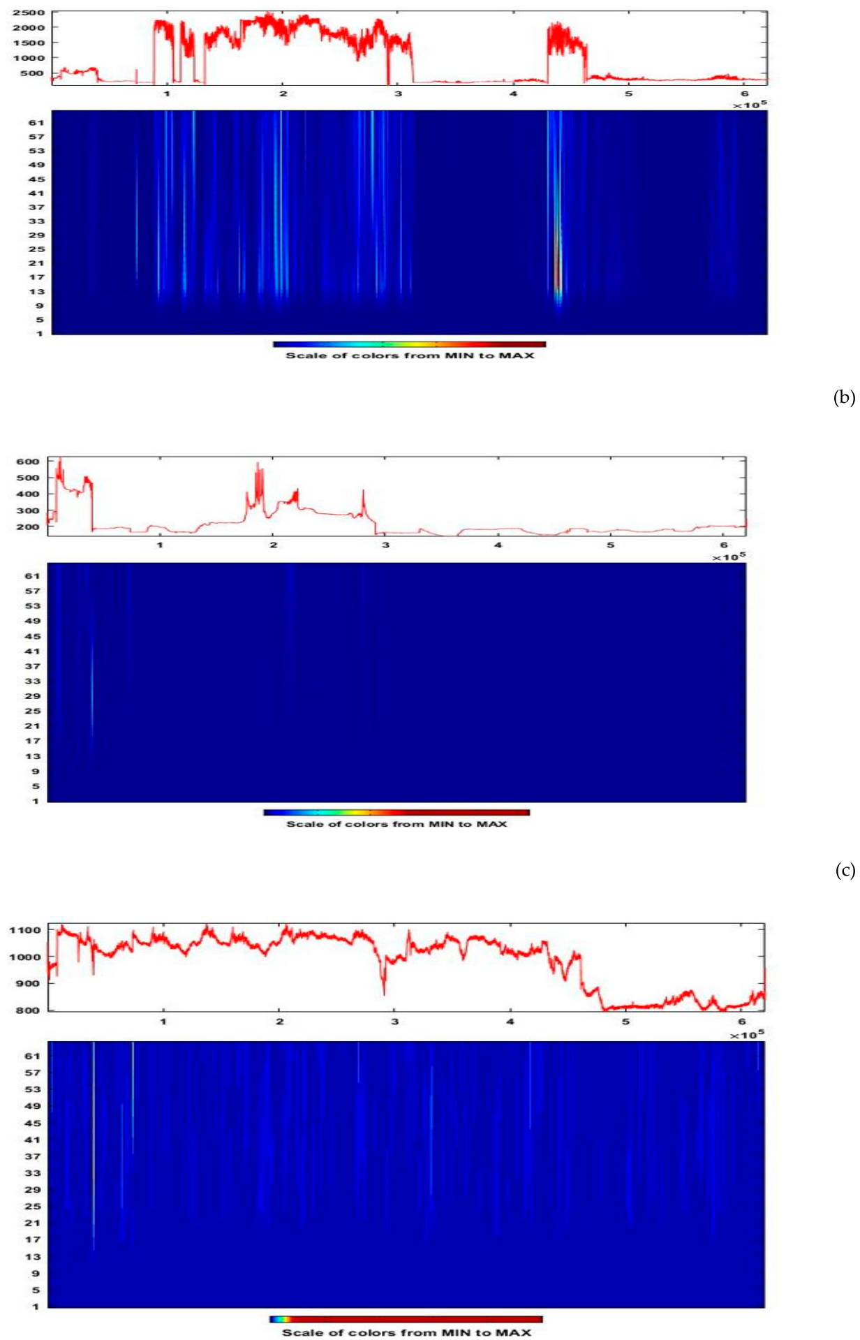
Figure 15.
CWT scalograms of MODWT-decomposed signal for 29 March earthquake: (a) CWT scalogram of 3 kHz MODWT decomposed signal; (b) CWT scalogram of 10 kHz MODWT decomposed signal; (c) CWT scalogram of 46 MHz MODWT decomposed signal
Figure 15.
CWT scalograms of MODWT-decomposed signal for 29 March earthquake: (a) CWT scalogram of 3 kHz MODWT decomposed signal; (b) CWT scalogram of 10 kHz MODWT decomposed signal; (c) CWT scalogram of 46 MHz MODWT decomposed signal
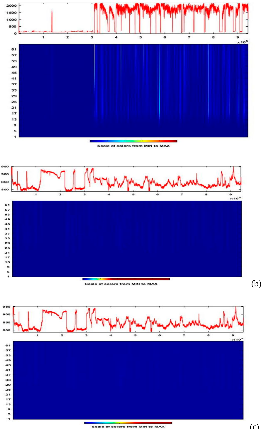
Figure 16.
CWT scalograms of MODWT-decomposed signal for 6 and 7 July earthquake: (a) CWT scalogram of 3 kHz MODWT decomposed signal; (b) CWT scalogram of 10 kHz MODWT decomposed signal; (c) CWT scalogram of 46 MHz MODWT decomposed signal.
Figure 16.
CWT scalograms of MODWT-decomposed signal for 6 and 7 July earthquake: (a) CWT scalogram of 3 kHz MODWT decomposed signal; (b) CWT scalogram of 10 kHz MODWT decomposed signal; (c) CWT scalogram of 46 MHz MODWT decomposed signal.
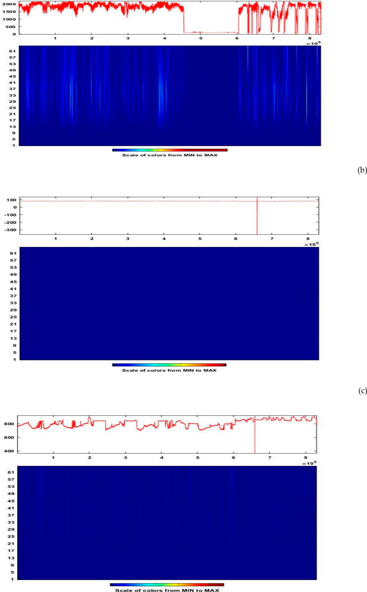
Figure 17.
CWT scalograms of MODWT-decomposed signal for 14 July earthquake: (a) CWT scalogram of 3 kHz MODWT decomposed signal; (b) CWT scalogram of 10 kHz MODWT decomposed signal; (c) CWT scalogram of 46 MHz MODWT decomposed signal.
Figure 17.
CWT scalograms of MODWT-decomposed signal for 14 July earthquake: (a) CWT scalogram of 3 kHz MODWT decomposed signal; (b) CWT scalogram of 10 kHz MODWT decomposed signal; (c) CWT scalogram of 46 MHz MODWT decomposed signal.
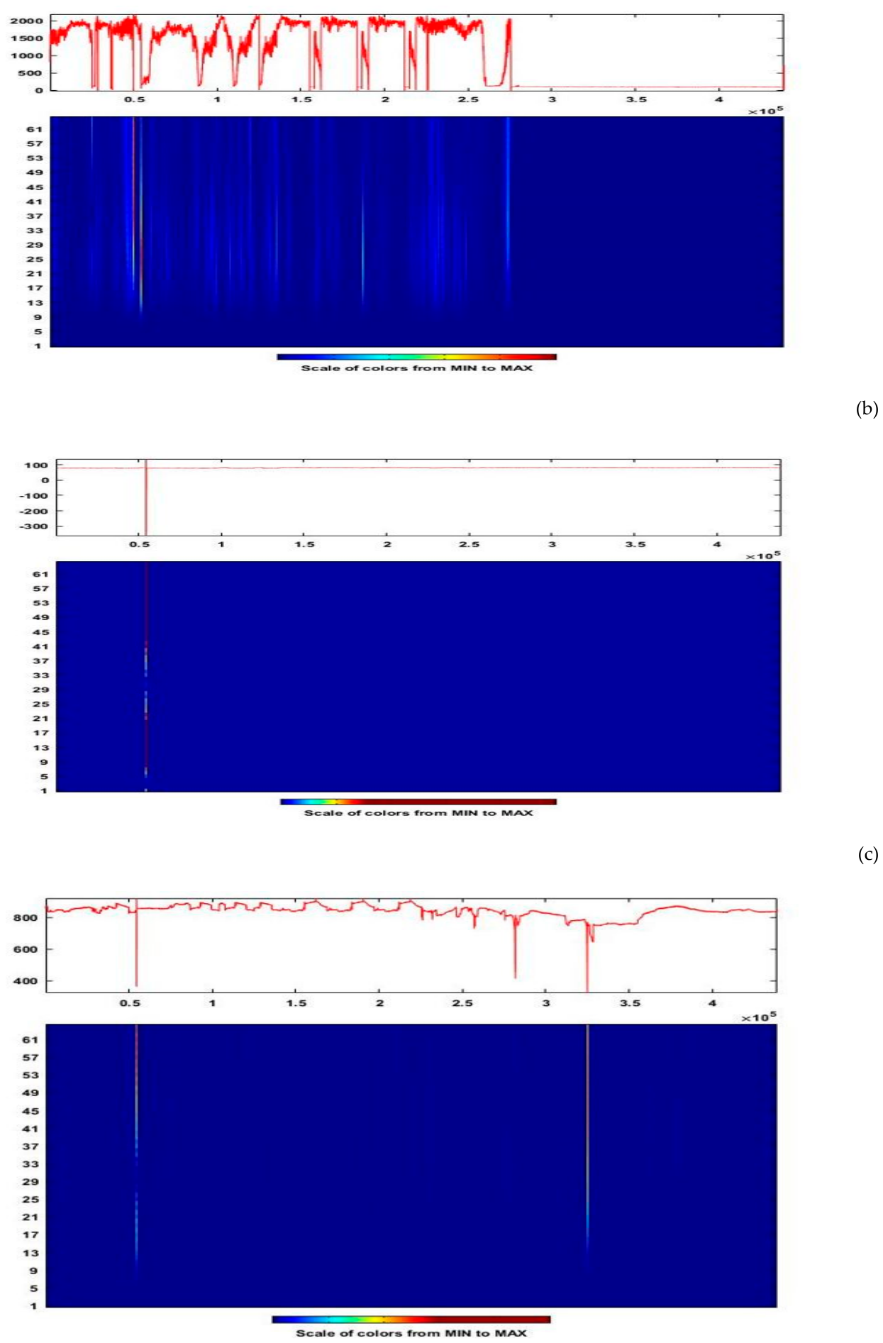
Figure 18.
CWT scalograms of MODWT-decomposed signal for 28 September earthquake: (a) CWT scalogram of 3 kHz MODWT decomposed signal; (b) CWT scalogram of 10 kHz MODWT decomposed signal; (c) CWT scalogram of 46 MHz MODWT decomposed signal.
Figure 18.
CWT scalograms of MODWT-decomposed signal for 28 September earthquake: (a) CWT scalogram of 3 kHz MODWT decomposed signal; (b) CWT scalogram of 10 kHz MODWT decomposed signal; (c) CWT scalogram of 46 MHz MODWT decomposed signal.
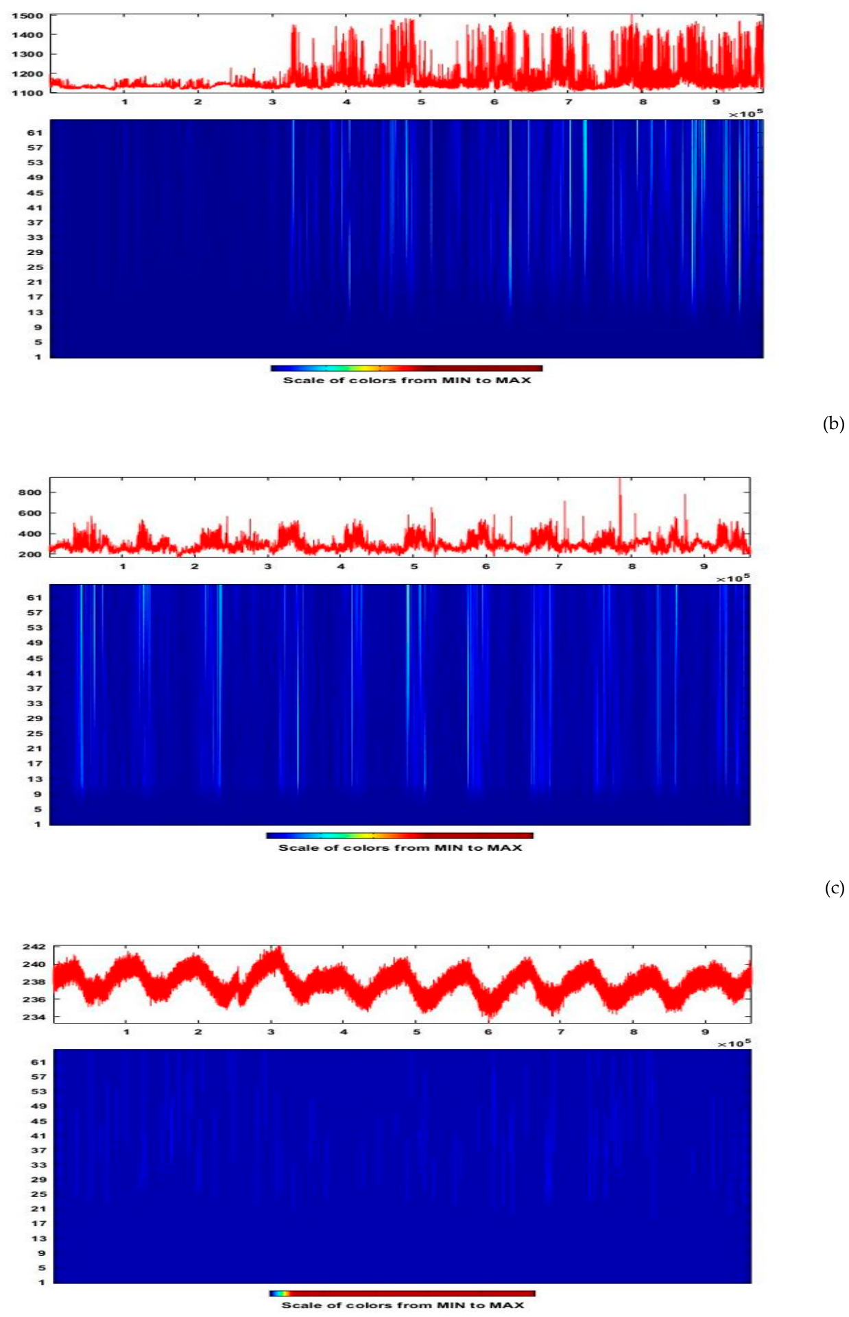
Figure 19.
CWT scalograms of MODWT-decomposed signal for 27 November earthquake: (a) CWT scalogram of 3 kHz MODWT decomposed signal; (b) CWT scalogram of 10 kHz MODWT decomposed signal; (c) CWT scalogram of 46 MHz MODWT decomposed signal.
Figure 19.
CWT scalograms of MODWT-decomposed signal for 27 November earthquake: (a) CWT scalogram of 3 kHz MODWT decomposed signal; (b) CWT scalogram of 10 kHz MODWT decomposed signal; (c) CWT scalogram of 46 MHz MODWT decomposed signal.
4. Conclusions
This study utilized a combined approach by using maximal overlap discrete wavelet transform (MODWT), continuous wavelet transform (CWT) and Hurst exponent to analyze the electromagnetic (EM) signals at distinct carrier frequencies of 3 kHz, 10 kHz and 46 MHz recorded over an 18-day window, 9 days before and after the eleven seismic events occurred during the study period. The objective of this study is to detect the unusual patterns potentially related to the seismic events occurred during the study and to evaluate the frequency dependence of EM precursors. Moreover, the persistent behavior of EM time series is analyzed through the Hurst exponent analysis.
The findings of this study show clear dependence of anomalies with the carrier frequency. At 3 kHz, the CWT scalograms of EM data for all seismic events exhibit distinct, localized energy clusters that are interpreted as seismic activity related EM precursors. The existence of anomalies at 3 kHz proposes that the earthquake occurrence involves irregular mechanical and electrical activity such as consecutive micro-fracturing events or atmospheric influences rather than steady, persistent emanation.
In contrast with 3 kHz signal, CWT scalograms of 10 kHz and 46 MHz EM signals exhibit inconsistent behavior across different seismic events. No coherent patterns are observed in EM data associated with the seismic events of 29th March (ML=4.1, ML=5.8, ML=3.5, ML=3.6 and ML=3.5), 6th and 7th July (ML=4.9 and ML=4.7) indicating the absence of anomalous patterns within the signal. Conversely, broader and diffused regions were observed in EM data associated with seismic events for 6th February (ML=3.9), 28 September (ML=4.4) and 27 November (ML=3.5). These features are neither well defined nor comprehensive so that they may be considered as clear pre-seismic signature. As some variability is present in 10 kHz and 46 MHz bands but the overall does not show clear temporal correlation of earthquakes was found.as it was affected with background noise or other external influences. The lack of detectable anomalies at 10 kHz and 46 MHz does not invalidate the methodology nor the physical veracity of pre-seismic emanations, in fact, it reflects the influence of several factors viz. spectral rolloff of emanation intensity with increasing frequency, greater EM attenuation at higher frequencies, and increased susceptibility to anthropogenic and natural noise contamination in these bands. Hurst exponent analysis revealed a frequency dependent response of EM signals. The 46 MHz signal consistently shows persistent behavior (H>0.5) throughout the study period whilst low frequency signals viz. 3 kHz and 10 kHz signals initially shows anti persistent behavior (H<0.5) but after 14 July seismic event they shows highly persistent behavior (H>0.5) indicating the structural organization of the signal.
Key findings reveal a strong frequency-dependent nature in anomaly detection performance. These findings underscores the critical importance of adapting signal processing techniques to the specific frequency characteristics of the input signal. Future research directions include: (1) investigating ensemble methods that combine multiple wavelet families, (2) developing adaptive algorithms that automatically adjust parameters based on signal characteristics, and (3) extending the methodology to additional frequency ranges and signal types. The demonstrated success of this approach offers promising applications across diverse domains including seismo-electromagnetic monitoring, telecommunications infrastructure diagnostics, and space weather research.
Supplementary Materials
The following supporting information can be downloaded at the website of this paper posted on Preprints.org.
Author Contributions
Conceptualization, D.N. and A.R..; methodology, D.N. and A.R,; software, A.R., C.D.; validation, M.R.,A.A.,S.D. K.K., N.G.,C.D.,M.P. and A.R..; formal analysis, A.R.,A.J.,N.G..,D.N.S.D.,K.K, M.R.,C.D.,M.P. and A.J.,; investigation, M.R.,A.R.,S.D.,D.N.,A.J.,N.G.,C.D.,M.P.,and K.K..; resources, D.N. and S.D..; data curation, D.N.A.R.,S.D.A.A.,N.G.., K.K.,C.D andA.J.; writing—original draft preparation, A.R.,M.R. and D.N. writing—review and editing, A.R.,A.J.,A.A.,N.G..,D.N.S.D.,K.K, M.R.,C.D., and A.J.,; visualization, A.R.; supervision, D.N..; project administration, D.N.;. All authors have read and agreed to the published version of the manuscript.”.
Funding:“This research received no external funding”.
Data Availability Statement
The raw data supporting the conclusions of this article will be made available by the authors on request.
Institutional Review Board Statement:“Not applicable”.
Data Availability Statement: We encourage all authors of articles published in MDPI journals to share their research data. In this section, please provide details regarding where data supporting reported results can be found, including links to publicly archived datasets analyzed or generated during the study. Where no new data were created, or where data is unavailable due to privacy or ethical restrictions, a statement is still required. Suggested Data Availability Statements are available in section “MDPI Research Data Policies” at https://www.mdpi.com/ethics.
Acknowledgments
In this section, you can acknowledge any support given which is not covered by the author contribution or funding sections. This may include administrative and technical support, or donations in kind (e.g., materials used for experiments).
Conflicts of Interest
Declare conflicts of interest or state “The authors declare no conflicts of interest.” Authors must identify and declare any personal circumstances or interest that may be perceived as inappropriately influencing the representation or interpretation of reported research results. Any role of the funders in the design of the study; in the collection, analyses or interpretation of data; in the writing of the manuscript; or in the decision to publish the results must be declared in this section. If there is no role, please state “The funders had no role in the design of the study; in the collection, analyses, or interpretation of data; in the writing of the manuscript; or in the decision to publish the results”.
References
- Dereszynski, E. W.; Dietterich, T. G. Spatiotemporal models for data-anomaly detection in dynamic environmental monitoring campaigns. ACM Trans. Sens. Netw. (TOSN) 2011, 8(1), 1–36. [Google Scholar] [CrossRef]
- Liu, H.; Zhang, X.; Dong, H.; Liu, Z.; Hu, X. Theories, applications, and expectations for magnetic anomaly detection technology: A review. EEE Sens. J. 2023, 23(16), 17868–17882. [Google Scholar] [CrossRef]
- Wang, Y.; Wu, Z.; Zhu, Y.; Zhang, P. Research on anomaly detection algorithm based on generalization latency of telecommunication network. Future Gener. Comput. Syst. 2018, 85, 9–18. [Google Scholar] [CrossRef]
- Cai, Y.; Shyu, M. L.; Tu, Y. X.; Teng, Y. T.; Hu, X. X. Anomaly detection of earthquake precursor data using long short-term memory networks. Appl. Geophys. 2019, 16(3), 257–266. [Google Scholar] [CrossRef]
- Mesarcik, M.; Boonstra, A. J.; Iacobelli, M.; Ranguelova, E.; De Laat, C. T. A. M.; Van Nieuwpoort, R. V. The road to discovery: Machine-learning-driven anomaly detection in radio astronomy spectrograms. Astron. Astrophys. 2023, A74. [Google Scholar] [CrossRef]
- Bulusu, J.; Arora, K.; Singh, S.; Edara, A. Simultaneous electric, magnetic and ULF anomalies associated with moderate earthquakes in Kumaun Himalaya. Nat. Hazards 2023, 116, 3925–3955. [Google Scholar] [CrossRef]
- Nikolopoulos, D.; Petraki, E.; Rafique, M.; Alam, A.; Cantzos, D.; Yannakopoulos, P. Fractal Features in kHz Electromagnetic Observations Preceding Near-Field Earthquakes in Ilia, Greece. Geosciences 2023, 13(12), 387. [Google Scholar] [CrossRef]
- Eftaxias, K.; Balasis, G.; Contoyiannis, Y.; Papadimitriou, C.; Kalimeri, M. Unfolding the procedure of characterizing recordedultra low frequency, kHZ and MHz electromagnetic anomalies prior to the L’Aquila earthquake as pre-seismic ones Part 2. Nat. Hazards Earth Syst. Sci. 2010, 10, 275–294. [Google Scholar] [CrossRef]
- Petraki, E. Electromagnetic Radiation and Radon-222 Gas Emissions as Precursors of Seismic Activity. Ph.D. Thesis, Department of Electronic and Computer Engineering, Brunel University, London, UK.
- Nikolopoulos, D.; Petraki, E.; Yannakopoulos, P.H.; Priniotakis, G.; Voyiatzis, I.; Cantzos, D. Long-lasting patterns in 3 kHz electromagnetic time series after the ML = 6.6 earthquake of 2018-10-25 near Zakynthos, Greece. Geosciences 2020, 10, 235. [Google Scholar] [CrossRef]
- Zong, J.; Tao, D.; Shen, X. Possible ELF/VLF Electric Field Disturbances Detected by Satellite CSES before Major Earthquakes. Atmosphere 2022, 13, 1394. [Google Scholar] [CrossRef]
- Yonaiguchi, N.; Ida, Y.; Hayakawa, M.; Masuda, S. Fractal analysis for VHF electromagnetic noises and the identification of preseismic signature of an earthquake. J. Atmos. Sol. Ter. Phys. 2007, 69, 1825–1832. [Google Scholar] [CrossRef]
- Smith, A.; Johnson, B.; Lee, C. Anomaly detection in electromagnetic spectra: A survey. IEEE Trans. Signal Process. 2020, 68(5), 1120–1135. [Google Scholar]
- Jones, R.; Brown, K. Limitations of Fourier Transform in transient signal analysis. J. Signal Process. 2019, 15(3), 45–60. [Google Scholar]
- Rasheed, A.; Osama, M.; Rafique, M.; Tareen, A. D. K.; Lone, K. J.; Qureshi, S. A.; Nikolopoulos, D. Time-frequency analysis of radon and thoron data using continuous wavelet transform. Phys. Scr. 2023, 98(10), 105008. [Google Scholar] [CrossRef]
- Liu, W.; Chen, W. Recent advancements in empirical wavelet transform and its applications. IEEE Access 2019, 7, 103770–103780. [Google Scholar] [CrossRef]
- Lee, D.H.; Lee, J.; Ahn, J.W. Mechanical vibration reduction control of two-mass permanent magnet synchronous motor using adaptive notch filter with fast fourier transform analysis. IET Electr. Power Appl. 2012, 6(7), 455–461. [Google Scholar] [CrossRef]
- Vanraj, S.; Dhami, B. Pabla, Hybrid data fusion approach for fault diagnosis of fixed-axis gearbox. Struct. Health Monit. 2018, 17(4), 936–945. [Google Scholar] [CrossRef]
- Zhao, H.; Liu, H.; Xu, J.; Guo, C.; Deng, W. Research on a fault diagnosis method of rolling bearings using variation mode decomposition and deep belief network. J. Mech. Sci. Technol. 2019, 33(9), 4165–4172. [Google Scholar] [CrossRef]
- Yang, H. Multiresolution mode decomposition for adaptive time series analysis. Appl. Comput. Harmon. Anal. 2021, 52, 25–62. [Google Scholar] [CrossRef]
- Tai, T. V.; Tan, M. P. N.; Tien, D. H.; Ha, N. V.; Hoang, T. T.; Pham, C. K.; Nguyen, T. T. T. A Novel ECG Signal Quality Index Method Based on Skewness-MODWT Analysis. IEEE Access 2024, 12, 70184–70197. [Google Scholar] [CrossRef]
- Zhang, H.; Wang, L.; Liu, G. Wavelet-based feature extraction for non-stationary signals. Signal Process. Lett. 2021, 28, 156–160. [Google Scholar]
- Qian, B.; Rasheed, K. Hurst exponent and financial market predictability. In Proceedings of the IASTED International Conference on Financial Engineering and Applications, Cambridge, MA, 2004; pp. 203–209. [Google Scholar]
- Hayakawa, M.; Hattori, K.; Nickolaenko, A. P.; Rabinowicz, L. M. Relation between the energy of earthquake swarm and the Hurst exponent of random variations of the geomagnetic field. Phys. Chem. Earth Parts A/B/C 2004, 29(4-9), 379–387. [Google Scholar] [CrossRef]
- Davis, G.H. Partitioned tectonic shortening, with emphasis on outcrop-scale folding and flattening, Pindos fold-and-thrust belt, Peloponnese, Greece. Can. J. Earth Sci. 2019, 56, 1181–1201. [Google Scholar] [CrossRef]
- Cataldi, G.; Villante, U.; De Lauretis, M.; Francia, P. ULF geomagnetic field measurements: Trends, disturbances, and signal analysis. J. Geophys. Res. Space Phys. 2021, 126((6)). [Google Scholar]
- Eftaxias, K.; Kopanas, J.; Bogris, N.; Kapiris, P.; Antonopoulos, G.; Varotsos, P. Detection of electromagnetic earthquake precursory signals in Greece. Proc.Japan Acad. Ser. B 2000, 76(4), 45–50. [Google Scholar] [CrossRef]
- Saini, K.; Dhami, S.S. MODWT and VMD based intelligent gearbox early stage fault detection approach. J. Fail. Anal. Prev. 2021, 21, 1821–1837. [Google Scholar] [CrossRef]
- Campo, D.; Quintero, O. L.; Bastidas, M. Multiresolution analysis (discrete wavelet transform) through Daubechies family for emotion recognition in speech. J. Phys.Conf. Ser. 2016, 705(1). [Google Scholar] [CrossRef]
- Kumar, A.; Joshi, L. K.; Pal, A.; Shukla, A. MODWT based time scale decomposition analysis of BSE and NSE indexes financial time series. Int. J. Math. Anal. 2011, 5(27), 1343–1352. [Google Scholar]
- Percival, D.B.; Walden, A.T. Wavelet methods for time series analysis; Cambridge University Press, 2000; Vol 4. [Google Scholar]
- Follis, J. L.; Lai, D. Variability analysis of epileptic EEG using the maximal overlap discrete wavelet transform. Health Inf. Sci. Syst. 2020, 8(1), 26. [Google Scholar] [CrossRef] [PubMed]
- Seo, Y.; Choi, Y.; Choi, J. River stage modeling by combining maximal overlap discrete wavelet transform, support vector machines and genetic algorithm. Water 2017, 9(7), 525. [Google Scholar] [CrossRef]
- Konar, P.; Saha, M.; Sil, J.; Chattopadhyay, P. Fault diagnosis of induction motor using CWT and rough-set theory. In 2013 IEEE Symposium on Computational Intelligence in Control and Automation (CICA); IEEE, April 2013; pp. pp. 17–23. [Google Scholar]
- Montejo, L.A.; Suarez, L.E. An improved CWT-based algorithm for the generation of spectrum-compatible records. Int. J. Adv. Struc. Eng. 2013, 5(1), 26. [Google Scholar] [CrossRef]
- Maji, C.; Sengupta, P.; Nandi, D.; Chaudhuri, H. SSRN 4234108; Hurst Exponent-Based Nonlinear Analysis for the Identification of Arrhythmia-Affected Cardiac Systems. 2021.
Disclaimer/Publisher’s Note: The statements, opinions and data contained in all publications are solely those of the individual author(s) and contributor(s) and not of MDPI and/or the editor(s). MDPI and/or the editor(s) disclaim responsibility for any injury to people or property resulting from any ideas, methods, instructions or products referred to in the content. |
© 2026 by the authors. Licensee MDPI, Basel, Switzerland. This article is an open access article distributed under the terms and conditions of the Creative Commons Attribution (CC BY) license.
Copyright: This open access article is published under a Creative Commons CC BY 4.0 license, which permit the free download, distribution, and reuse, provided that the author and preprint are cited in any reuse.