

Submitted:
02 November 2026
Posted:
04 November 2026
You are already at the latest version
Abstract
Income and education capture distinct but interrelated dimensions of socioeconomic resources. This study examines the association between the family income-to-poverty ratio (PIR) and measured systolic blood pressure (SBP), comparing estimates before and after adjustment for body mass index (BMI) and education. Four NHANES components were linked, and eligibility, repeated measurements, pregnancy status and variable completeness were assessed to obtain a common sample of 5019 adults. Three linear models incorporated examination weights, strata and primary sampling units, sequentially adjusting for demographic characteristics, BMI and education. Each one-unit higher PIR was associated with an SBP difference of -0.682 mmHg after demographic adjustment (95% CI -1.193 to -0.171), -0.656 after adding BMI (-1.193 to -0.119), and -0.201 after adding education (-1.014 to 0.612). Education adjustment substantially attenuated the income gradient, whereas BMI adjustment changed it little. Presenting these models together shows how the interpretation of income-related blood pressure differences depends on the dimensions of social resources included in the comparison.
Keywords:
social inequalities in health
; Income-to-Poverty Ratio (PIR)
; education
; systolic blood pressure
; complex survey
; R language
1. Introduction
Whether people with higher incomes have lower blood pressure is an intuitive public health question. Addressing it requires distinguishing income from population composition and educational resources. Income can influence housing, diet and access to healthcare, while education is associated with occupational opportunities, health literacy and social networks. The social determinants of health framework places these conditions among the important sources of health differences [5,6,7]. The challenge is to specify the conditions under which comparisons are made. Income, education and body composition are interrelated within a population, and adding covariates changes the conditional relationship represented by a regression coefficient. If models use different samples, coefficient differences may also reflect changes in sample composition. This study therefore holds the sample constant while comparing income gradients under progressively richer adjustment.
The research question is how the demographically adjusted income–SBP association changes when BMI and education are added in the same sample. Measured continuous SBP from 2021-2023 cycle provides an interpretable outcome. Linking sample construction, survey design and sequential adjustment allows these changes to be compared directly within one results table.
1.1. Research Context and Analytical Framework
Previous studies approach this question from different perspectives. Assari examined education, income and continuous SBP in NHANES, including racial and ethnic differences [8]. Calixte and colleagues investigated education, sex and age-related blood pressure trajectories using linear and quadratic regression specifications [9]. Reeves and Odden studied hypertension subtypes using multinomial logistic regression, illustrating that continuous blood pressure and categorical outcomes address different questions [10]. Studies from China and India connect socioeconomic status with hypertension incidence, diagnosis and body composition [11,12,13]. These studies highlight the importance of specifying both the outcome and the adjustment conditions when interpreting income coefficients. Income and education represent related dimensions of social resources. The demographically adjusted income gradient captures the correspondence of economic resources and their associated circumstances with blood pressure. After education is included, the comparison concerns income differences at a given educational level. Reporting both comparisons makes this shift in interpretation visible.
Figure 1 below organizes the analysis into data preparation, common-sample modelling and interpretation. Models M1, M2 and M3 sequentially add adjustment variables, supported by survey-based inference, diagnostics and specification checks. Arrows indicate the sequence of analytical steps; the dashed enclosure groups the six central modelling and evaluation components.
2. Data and Methods
2.1. Data Sources and Sample Construction
The data come from the publicly available August 2021-August 2023 NHANES cycle [1]. DEMO_L supplies demographic characteristics, family income, education and survey design variables. BPXO_L contains repeated automated blood pressure measurements. BMX_L contains body measurements and BPQ_L contains blood pressure questionnaire data [2,3,4]. After confirming that participant identifier SEQN was unique within each component, one-to-one left joins anchored to DEMO_L produced an intermediate dataset of 11933 participants and 29 variables. Questionnaire fields were retained for traceability, while the regression outcome was derived from examination measurements.
Figure 2 below shows the filtering process of the data cleaning, and each count denotes participants meeting all preceding and current criteria.
Sample selection followed a consistent sequence. 8860 participants had valid examination and design information, 6064 were aged at least 20 years, and 5857 had at least two valid SBP measurements. Excluding 39 participants with known pregnancy left 5818. Requiring observed PIR, BMI and education sequentially reduced the sample to 5068, 5020 and 5019. The final sample represented 86.3% of the eligible study population. All models used these same participants so that sample changes would not confound comparisons of coefficients. Components were linked at the participant level rather than the measurement level. The 29-variable intermediate dataset retained component-presence indicators and repeated readings for source checks. The final modelling dataset retained the study variables and design fields, connecting each selection step to subsequent estimation.
2.2. Variable Definitions and Complete-Record Strategy
The outcome was the mean of at least two valid SBP readings. Checks identified non-positive readings, values above 300 mmHg, and readings in which SBP did not exceed the paired diastolic pressure. A valid SBP reading was retained when its paired diastolic reading was missing. PIR describes family income relative to the applicable poverty threshold, where the released value of 5 represents 5 or above. Age 80 represents 80 years or older. Published BMI values were used, with non-positive or non-finite values treated as missing. Refused and unknown education codes were recoded as missing.
Repeated valid measurements were combined into a continuous participant-level outcome. denotes the set of valid readings for participant and their number. The requirement of at least two readings was consistent across models. PIR, age and BMI retained their published scales, and categorical codes were converted to factors before estimation. Sex, race/ethnicity and education entered as categorical variables. Reference categories were men, non-Hispanic White participants and high school/GED, respectively. Education had five categories, including (1) less than ninth grade, (2) ninth to eleventh grade, (3) high school/GED, (4) some college or an associate degree, (5) a college degree or above.
The final dataset comprised 11 fields, including (1) participant identifier, (2) SBP, (3) PIR, (4) age, (5) sex, (6) race/ethnicity, (7) BMI, (8) education and (9-11) three design variables. None of these fields contained missing values in the final sample.
Complete-record analysis retained observed values and described the composition of excluded records separately [16,20]. Among the 5818 eligible participants, 750 had missing PIR. A further 48 had observed PIR but missing BMI, followed by one exclusion for missing education. Non-Hispanic White participants accounted for 50.3% of the missing-PIR group, compared with 62.4% of the included sample, indicating a change in social composition. No mean PIR was estimated for the missing-PIR group because it had no observed PIR values.
Table 1 reports actual denominators for each variable. Of the 750 participants with missing PIR, 741 had observed BMI and 749 had observed college-education status. Their PIR entry is blank because no PIR values were observed. Mean age was similar between groups, whereas racial and ethnic composition differed more noticeably. This comparison characterizes the coverage of the complete-record sample.
2.3. Sequential Regression in a Common Sample
Let denote mean SBP, P denote PIR, denote age minus 50, denote sex, denote race/ethnicity indicators, denote BMI minus 30, and denote education indicators. The three models are:
M1 estimates the income association adjusted for age, sex and race/ethnicity, and M2 adds BMI and M3 adds education. All coefficients are re-estimated in each model. Education adjustment changes the comparison: M1 and M2 retain information that varies jointly with income and education, whereas M3 compares income conditional on education. These models progressively refine the comparison. M1 contrasts mean blood pressure across PIR values at the same demographic characteristics, M2 additionally holds BMI constant, and M3 also holds educational category constant. Each addition changes the comparison conditions and reallocates the variation described by the explanatory variables.
Weighted least squares used examination weight WTMEC2YR, allowing participants to contribute according to their population representation. The objective function is:
is the diagonal matrix of examination weights, and contains the intercept and explanatory variables. Differentiating the weighted residual sum of squares and setting the derivative to zero gives the normal-equation solution above. Weighted fitting determines the coefficients, while the sampling structure informs variance estimation. Centering age and BMI changes the interpretation of the intercept without changing the PIR slope or fitted values.
2.4. Complex Survey Design and Statistical Inference
The design was first constructed for the 8860 participants with valid examination information, after which the 5019 complete records were defined as an analysis domain. SDMVSTRA and SDMVPSU identified strata and primary sampling units (PSUs), with PSUs nested within strata. Variances were estimated by Taylor linearization using survey [14,15]. This cycle contained 15 variance strata and 30 PSUs, giving 15 design degrees of freedom. Weights, strata and PSUs serve distinct functions. Examination weights describe population representation, strata record the grouping used in sampling, and PSUs preserve the dependence structure of information within primary sampling units. Incorporating these features aligns sampling-error estimation with the way the data were collected.
Taylor linearization approximates variation in regression estimates through PSU-level contributions and aggregates them within strata. Statistical precision therefore depends on independent sampling information as well as model specification. The 5,019 records provide participant-level information, while the 15 design degrees of freedom summarize the sampling structure available for design-based inference.
Results include income coefficients, design-based standard errors, two-sided values and 95% confidence intervals. The default residual design degrees of freedom in survey were 7, 6 and 2 respectively for M1, M2 and M3. Intervals used the corresponding distributions. values were interpreted alongside effect sizes rather than as a stand-alone assessment of model suitability [18]. denotes the design-based standard error.
The test statistic compares the coefficient with its standard error, and the confidence interval uses the critical value for the relevant degrees of freedom. The models contain 8, 9 and 13 non-intercept parameters, respectively, leaving 7, 6 and 2 residual degrees of freedom. Five educational categories require four indicators, making limited degrees of freedom particularly relevant to precision in M3. Coefficient magnitude, interval width and values provide complementary information. Coefficients describe associations in mmHg, intervals indicate precision, and values characterize compatibility with a zero coefficient under the test specification [18]. Presenting all three makes changes in the income gradient distinguishable from changes in statistical precision.
2.5. Implementation
All statistical analyses and figures were produced in R, using survey for regression and haven for data import and export [15]. Scripts retain the original XPT files and implement linkage, cleaning and construction of the final dataset. A common sample, outcome definition and weighting scheme underpin the main comparisons. Diagnostics and specification checks assess residual structure, collinearity, age functions and stratum influence. Sample flow, variable definitions and reporting follow STROBE principles [19].
3. Results
3.1. Sample Characteristics and Unadjusted Income Differences
Participants had a weighted mean SBP of 121.43 mmHg, PIR of 3.05 and BMI of 29.67. Approximately half were women and 35% had a college degree or above. Descriptive statistics and regression estimates use the same participants, which supports consistent interpretation across results.

Table 2.
Survey-weighted characteristics of the common analytical sample ().
| Characteristic | Weighted estimate | 95% CI |
|---|---|---|
| Age (years) | 49.10 | 47.98 to 50.22 |
| SBP (mmHg) | 121.43 | 120.54 to 122.33 |
| PIR | 3.05 | 2.84 to 3.27 |
| BMI (kg/m²) | 29.67 | 29.08 to 30.26 |
| Women (%) | 50.68 | 49.28 to 52.07 |
| Non-Hispanic White (%) | 62.37 | 58.14 to 66.60 |
| College degree or above (%) | 35.20 | 28.42 to 41.99 |
Figure 3.
Unadjusted survey-weighted mean SBP and 95% confidence intervals by PIR group.
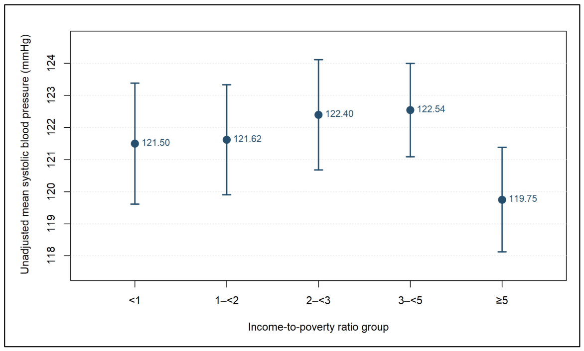
Mean blood pressure did not decrease monotonically across the middle-income groups, while the highest-income group had the lowest mean. These unadjusted means also reflect differences in age, sex and other population characteristics, which the regression models subsequently address.
3.2. Changes in Income Coefficients Across Models
In M1, each one-unit higher PIR was associated with 0.682 mmHg lower mean SBP. After BMI adjustment, the difference was 0.656 mmHg, a movement toward zero of 0.026 mmHg, or approximately 3.8%. Further education adjustment yielded a coefficient of −0.201, with a 95% confidence interval from −1.014 to 0.612. Figure 4 compares the three estimates.
In M3, participants with a college degree or above had an estimated SBP difference of −3.488 mmHg relative to the high school/GED group (95% CI −5.877 to −1.099). Weighted in-sample values were 0.195, 0.197 and 0.204. Education adjustment modestly increased explained variation while attenuating the income gradient, describing two different aspects of model performance. The movement from −0.656 in M2 to −0.201 in M3 shows that educational information changes the income comparison.
The income variable and its units are unchanged, and the models use the same participants, and the shift arises when education is added to the adjustment set.
3.3. Adjusted Curves and the Magnitude of Blood Pressure Differences
The adjusted curves retain the weighted distribution of other covariates while showing average fitted SBP at each PIR value. Increasing PIR from 1 to 4 corresponds to estimated mean differences of approximately −2.045, −1.968 and −0.603 mmHg in M1, M2 and M3, respectively. These contrasts express the coefficient changes as directly interpretable population comparisons. At each PIR value, the fitted equation is applied to every participant in the common sample, and the predictions are averaged using examination weights. Holding the distribution of other variables constant provides a consistent background for comparisons. Figure 5 and Table 3 express the same result: M1 and M2 have similar slopes, while M3 is flatter.
One PIR unit represents an increase of one poverty-threshold multiple in family income, and its monetary equivalent varies with the applicable threshold, including family composition. Comparing PIR 1 with PIR 4 places the small blood pressure gradient across a wider socioeconomic distance, approximately 2.05 mmHg in M1 and 0.60 mmHg after education adjustment. The shaded regions convey precision. Although M3 has a flatter estimated slope, its interval is wider because additional educational parameters reduce residual degrees of freedom. The slope describes association magnitude, while shading describes uncertainty in the estimated mean.
3.4. Residual Structure and Collinearity
Residuals are differences between observed mean SBP and fitted values. The upper panels of Figure 6 plot residuals against fitted values, while the lower panels compare sample and normal quantiles. All three models show a positive tail, with some high readings substantially above the modelled mean. Adding education changes the overall residual shape little. The following formula calculates the residuals of the predicted results.
Figure 6 displays participant-level observations. Formal standard errors incorporate the complex sampling structure. Residual skewness is approximately 0.73-0.74. Sequential adjustment primarily modifies the mean structure, while the positive tail of high SBP readings remains. Residual plots describe this performance, and design-based variance estimation addresses sampling dependence. Weighted design-matrix diagnostics give a PIR VIF of 1.424 in M3 and an education GVIF of 1.506, or 1.053 after adjustment for its four degrees of freedom [17]. These values do not indicate severe linear dependence. The attenuation after education adjustment is therefore interpreted in terms of shared social resources and the conditional comparison.
3.5. Age Specifications and Stratum Influence
Age specifications were compared in the same 5019 participants. M1 and M2 were refitted with an age-squared term or a natural cubic spline with internal knots at 40 and 60 years and boundaries at 20 and 80. Figure 7 and Table 4 compare income coefficients and precision across these forms.
M1 coefficients ranged from -0.682 to -0.649 and M2 coefficients from -0.656 to -0.609. Point estimates changed little, but the M2 spline interval was -1.256 to 0.039, including zero. Additional parameters reduced residual degrees of freedom and changed interval widths. Age-form comparisons focused on M1 and M2 because M3 retained two residual degrees of freedom. Omitting each complete sampling stratum in turn yielded income coefficients ranging from -0.755 to -0.610 in M1, -0.731 to -0.579 in M2, and -0.276 to -0.103 in M3. No direction reversal was observed. This check evaluates dependence on individual strata, complementing the assessment of age functional form.
4. Discussion
The central finding is that the income gradient changes after education adjustment. Higher PIR was associated with slightly lower SBP after demographic and BMI adjustment, whereas the association attenuated when education entered the model.
Income and education are linked but represent different resources. Education may relate to health literacy, occupational conditions and healthcare navigation, while income concerns purchasing power, housing choices and daily constraints. In M3, the income coefficient approached zero and college graduates had lower SBP than the high school/GED group. These results align with the social determinants framework [5,6,7], in which education forms part of the context for interpreting economic resources and health. Presenting the models together preserves both the broader income gradient and the comparison conditional on education.
The attenuation reflects a change in coefficient magnitude as well as statistical significance. Adding education shifted the PIR estimate from -0.656 to -0.201, while its standard error decreased from 0.219 to 0.189. The wider confidence interval also reflects the reduction in residual degrees of freedom from six to two and the resulting larger critical value. Changes in the slope and interval width thus have different sources. A one-unit PIR contrast of 0.68 mmHg is small, comparing PIR 1 with PIR 4 expresses the same M1 gradient as approximately 2.05 mmHg. From a public health perspective, the results motivate closer examination of resources that vary within educational groups and resources that vary jointly with education, including occupational conditions, living environments and access to care.
Complete-record analysis provides a consistent set of observed measurements but limits coverage through item nonresponse. Participants with missing income differed in racial and ethnic composition, and their true PIR was unobserved. Examination weights address sampling and some survey nonresponse but do not automatically correct selection from item missingness [16,20]. The cross-sectional design describes contemporaneous conditional associations. Top-coded PIR and age, incomplete treatment and lifestyle information, and limited design degrees of freedom further shape interpretation. Future analyses can examine missing-data coverage, treatment status and the measurement of social resources, building on the transparent comparison provided here.
5. Conclusions
Among 5019 adults with complete records in NHANES 2021–2023, each one-unit higher PIR was associated with approximately 0.68 mmHg lower mean SBP after demographic adjustment and 0.66 mmHg lower SBP after adding BMI. Further education adjustment attenuated the income coefficient to approximately -0.20 mmHg. Interpretation of the income gradient therefore depends on whether educational resources are considered. A common sample, complex-survey estimation and parallel reporting make this change explicit and provide a reproducible analysis of socioeconomic conditions and blood pressure differences.
Appendix A. Data & Code
The source data are the publicly available NHANES 2021–2023 files. Component documentation is provided in references [1,2,3,4].
Analysis code, variable definitions and reproducibility materials are provided in the accompanying project repository https://github.com/YQY444/NHANES-Social-Data-Science-Public-Health
References
- Terry, A.L.; Chiappa, M.M.; McAllister, J.; Woodwell, D.A.; Graber, J.E. Plan and operations of the National Health and Nutrition Examination Survey August 2021–August 2023; Vital and Health Statistics Series; 2024. [Google Scholar] [CrossRef]
- National Center for Health Statistics. NHANES August 2021–August 2023 Demographic Variables and Sample Weights DEMO_L. Data documentation. 2024. (accessed on 29 October 2026).
- National Center for Health Statistics. NHANES August 2021–August 2023 Blood Pressure Oscillometric Measurements BPXO_L. Data documentation. 2024. (accessed on 29 October 2026).
- National Center for Health Statistics. NHANES August 2021–August 2023 Body Measures BMX_L. Data documentation. 2024. (accessed on 29 October 2026).
- Marmot, M. Social determinants of health inequalities. Lancet 2005, 365, 1099–1104. [Google Scholar] [CrossRef] [PubMed]
- Braveman, P.; Gottlieb, L. The social determinants of health: it's time to consider the causes of the causes. Public Health Rep. 2014, 129, 19–31. [Google Scholar] [CrossRef] [PubMed]
- Link, B.G.; Phelan, J. Social conditions as fundamental causes of disease. J. Health Soc. Behav. 1995. [Google Scholar] [CrossRef] [PubMed]
- Assari, S. Socioeconomic determinants of systolic blood pressure; minorities' diminished returns. J. Health Econ. Dev. 2019, 1, 1–11. [Google Scholar] [PubMed]
- Calixte, R.; Besson, A.; Chahal, K.; Kaplan, M.S. Education differences in blood pressure trajectories by sex through midlife: findings from the National Health and Nutrition Examination Survey, 1999–2018. Blood Press Monit. 2025, 30, 1–10. [Google Scholar] [CrossRef] [PubMed]
- Reeves, A.N.; Odden, M.C. Racial disparities in hypertension subtype prevalence over the lifecourse: evidence of accelerated arterial ageing in a population representative cross-sectional study. BMJ Public Health 2025, 3, e001993. [Google Scholar] [CrossRef] [PubMed]
- Luo, T.; Lin, S.; Zhang, W.; et al. Relationship between socioeconomic status and hypertension incidence among adults in southwest China: a population-based cohort study. BMC Public Health 2024, 24, 1211. [Google Scholar] [CrossRef] [PubMed]
- Bhatia, M.; Dixit, P.; Kumar, M.; Dwivedi, L.K. Comparing socio-economic inequalities in self-reported and undiagnosed hypertension among adults 45 years and over in India: what explains these inequalities? Int. J. Equity Health 2023, 22, 26. [Google Scholar] [CrossRef] [PubMed]
- Li, Y.; Ge, W.; Wu, M.; et al. Association between socioeconomic status and hypertension among adults in Fujian province and the mediating effect of BMI and cooking salt intake: a cross-sectional study. BMJ Open 2024, 14, e076785. [Google Scholar] [CrossRef] [PubMed]
- Lumley, T.; Scott, A. Fitting regression models to survey data. Stat. Sci. 2017, 32, 265–278. [Google Scholar] [CrossRef]
- Lumley, T. Analysis of complex survey samples. J. Stat. Softw. 2004, 9, 1–19. [Google Scholar] [CrossRef]
- Sterne, J.A.C.; White, I.R.; Carlin, J.B.; et al. Multiple imputation for missing data in epidemiological and clinical research: potential and pitfalls. BMJ 2009, 338, b2393. [Google Scholar] [CrossRef]
- Fox, J.; Monette, G. Generalized collinearity diagnostics. J. Am. Stat. Assoc. 1992, 87, 178–183. [Google Scholar] [CrossRef]
- Wasserstein, R.L.; Lazar, N.A. The ASA's statement on p-values: context, process, and purpose. Am. Stat. 2016, 70, 129–133. [Google Scholar] [CrossRef]
- von Elm, E.; Altman, D.G.; Egger, M.; Pocock, S.J.; Gøtzsche, P.C.; Vandenbroucke, J.P. The Strengthening the Reporting of Observational Studies in Epidemiology (STROBE) statement: guidelines for reporting observational studies. PLoS Med. 2007, 4, e296. [Google Scholar] [CrossRef] [PubMed]
- Carpenter, J.R.; Smuk, M. Missing data: a statistical framework for practice. Biom. J. 2021, 63, 915–947. [Google Scholar] [CrossRef] [PubMed]
Figure 1.
Overall analytical framework.
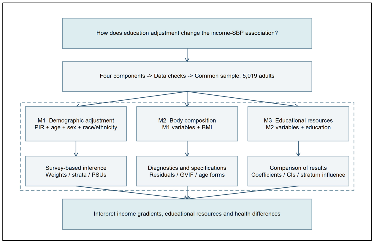
Figure 2.
Sequential sample filtering.
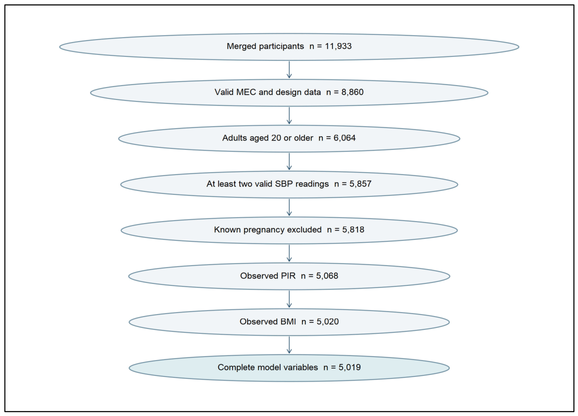
Figure 4.
Income coefficients and 95% confidence intervals across sequential models.
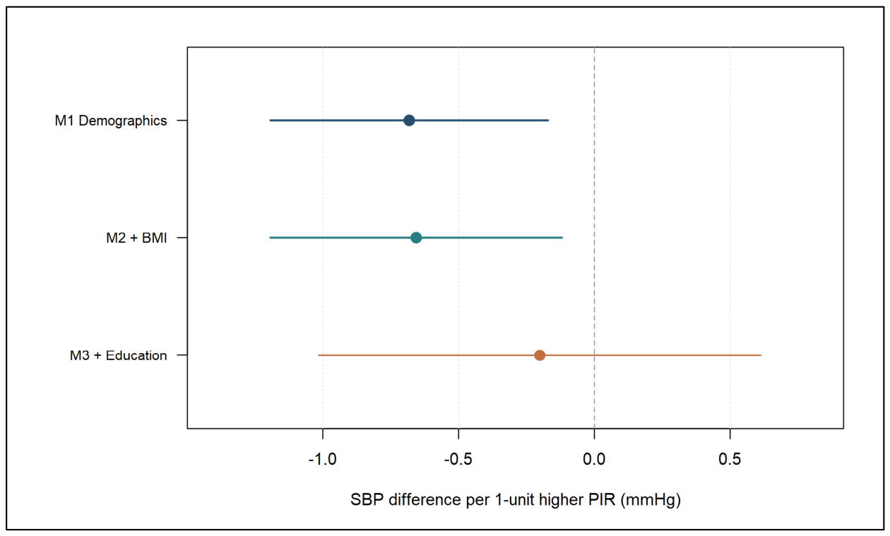
Figure 5.
Mean SBP standardized to the weighted covariate distribution of the common sample.
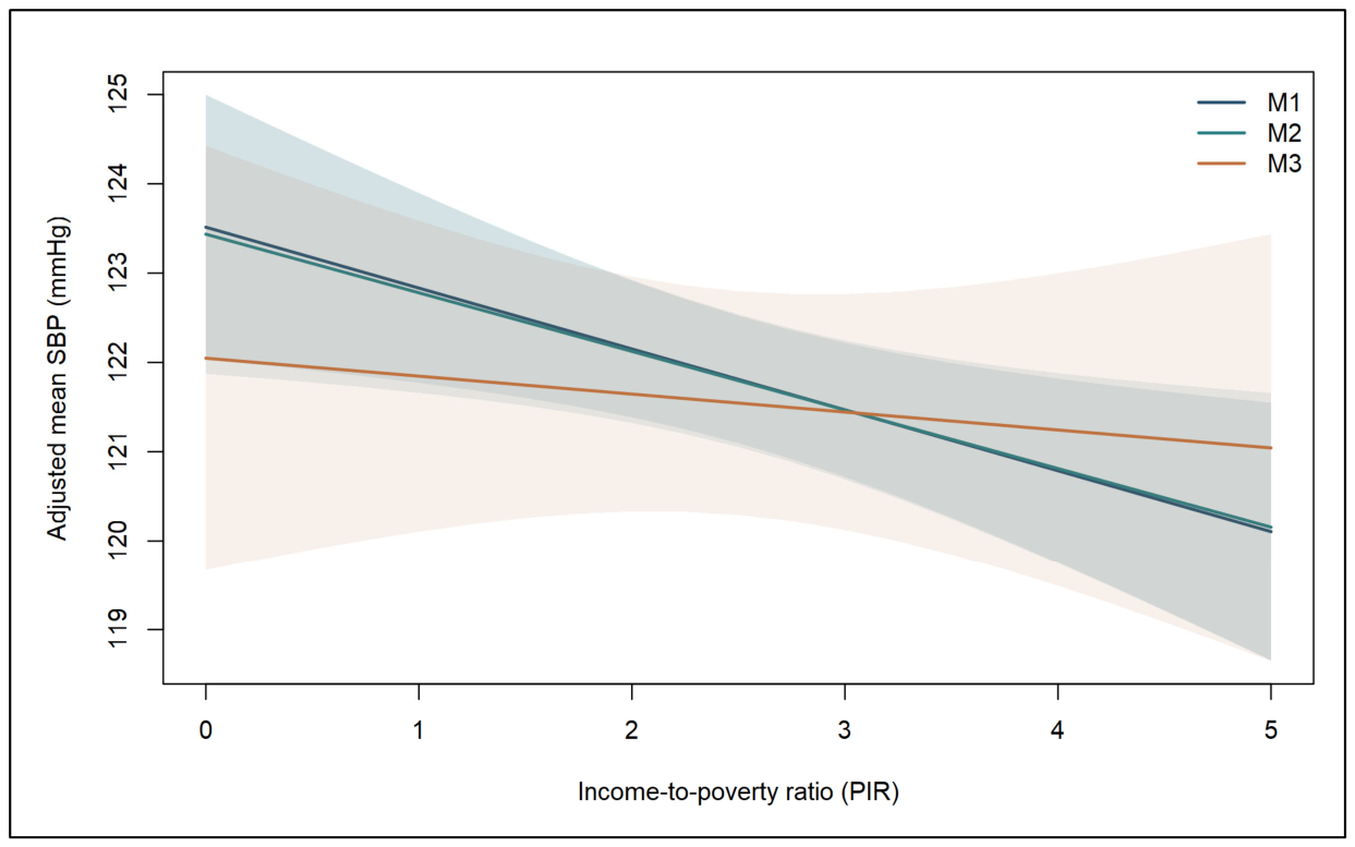
Figure 6.
Residual-fitted plots and normal Q-Q plots for the three models.
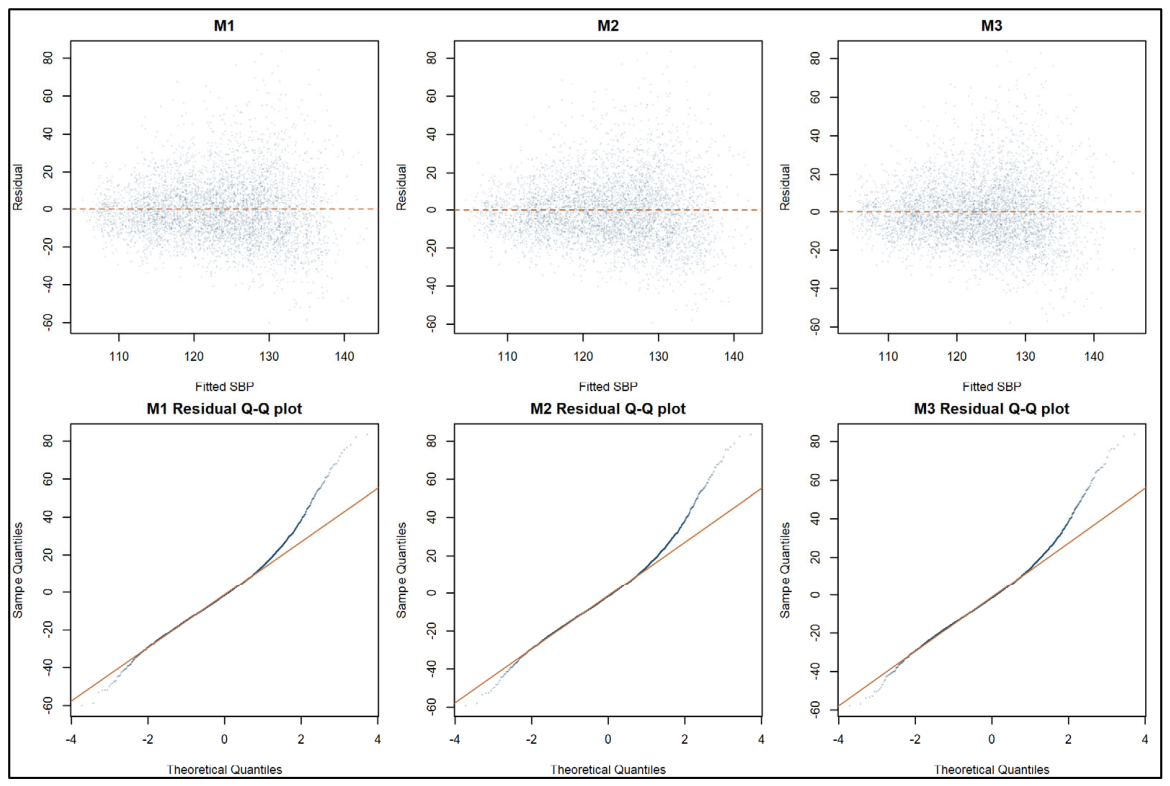
Figure 7.
PIR coefficients and 95% confidence intervals under three age specifications in M1 and M2.
Figure 7.
PIR coefficients and 95% confidence intervals under three age specifications in M1 and M2.
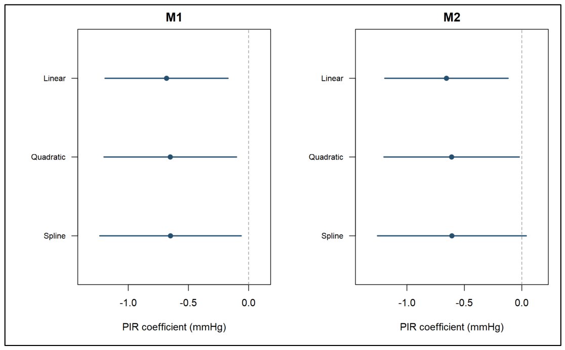
Table 1.
Survey-weighted characteristics of included participants and those with missing PIR.
| Characteristic | Included | Missing PIR |
|---|---|---|
| Age (years) | 49.10 (n=5019) | 48.69 (n=750) |
| SBP (mmHg) | 121.43 (n=5019) | 119.90 (n=750) |
| PIR | 3.05 (n=5019) | - (n=0) |
| BMI | 29.67 (n=5019) | 29.15 (n=741) |
| Non-Hispanic White (%) | 62.37 (n=5019) | 50.28 (n=750) |
| College degree or above (%) | 35.20 (n=5019) | 28.95 (n=749) |
Table 3.
PIR coefficients in the common sample of 5,019 adults, in mmHg.
| Model | PIR coefficient | Design SE | 95% CI | value |
|---|---|---|---|---|
| M1 | -0.682 | 0.216 | -1.193 to -0.171 | 0.0160 |
| M2 | -0.656 | 0.219 | -1.193 to -0.119 | 0.0243 |
| M3 | -0.201 | 0.189 | -1.014 to 0.612 | 0.3988 |
Table 4.
Point estimates and precision under alternative age specifications.
| Model and age specification | PIR coefficient | 95% CI | value | |
|---|---|---|---|---|
| M1 Linear | -0.682 | -1.193 to -0.171 | 0.0160 | 7 |
| M2 Linear | -0.656 | -1.193 to -0.119 | 0.0243 | 6 |
| M1 Quadratic | -0.651 | -1.201 to -0.100 | 0.0276 | 6 |
| M1 Natural spline | -0.649 | -1.236 to -0.062 | 0.0362 | 5 |
| M2 Quadratic | -0.611 | -1.200 to -0.022 | 0.0445 | 5 |
| M2 Natural spline | -0.609 | -1.256 to 0.039 | 0.0594 | 4 |
Disclaimer/Publisher’s Note: The statements, opinions and data contained in all publications are solely those of the individual author(s) and contributor(s) and not of MDPI and/or the editor(s). MDPI and/or the editor(s) disclaim responsibility for any injury to people or property resulting from any ideas, methods, instructions or products referred to in the content. |
© 2026 by the authors. Licensee MDPI, Basel, Switzerland. This article is an open access article distributed under the terms and conditions of the Creative Commons Attribution (CC BY) license (http://creativecommons.org/licenses/by/4.0/).
Copyright: This open access article is published under a Creative Commons CC BY 4.0 license, which permit the free download, distribution, and reuse, provided that the author and preprint are cited in any reuse.