

Submitted:
03 November 2026
Posted:
04 November 2026
You are already at the latest version
Abstract
Financial time-series forecasting is commonly optimized with mean squared error (MSE), yet volatility clustering, heavy tails, and regime shifts make a fixed quadratic objective poorly suited. Existing robust losses improve resistance to extreme errors but lack adaptive volatility normalization and explicit directional supervision, while directional objectives such as Generalized Mean Absolute Directional Loss (GMADL) do not integrate volatility scaling, tail adaptation, and noise-aware directional weighting. We introduce Regime-Normalized Adaptive Directional Loss (RNAD), a model-agnostic training objective combining online volatility normalization via batch-scale estimates and an exponential moving average, tail-gated interpolation between quadratic and Charbonnier penalties, and noise-gated directional supervision that attenuates near-zero returns. RNAD requires no architectural changes, adds only a scalar state buffer, and incurs no inference-time overhead. Across nine financial assets, four architectures (PatchTST, iTransformer, N-HiTS, TimeXer), five losses, and three seeds under chronological splits, RNAD achieves the lowest mean RMSE for every backbone, reducing RMSE by 0.086–0.882 units versus the strongest non-RNAD baseline. It also improves MAE and directional accuracy (DA), with the lowest RMSE on all nine assets when paired with PatchTST. Four-step forecasts on US500 and USDJPY improve average DA by 2.39 and 1.41 percentage points, respectively, and reduce flattened RMSE on US500 by 0.3%. Ablations identify directional supervision as the main contributor, with tail adaptation and noise gating providing complementary, regime-dependent gains. Overall, adaptive, volatility-aware loss design offers a lightweight route to better numerical accuracy and directional consistency across financial forecasting architectures.
Keywords:
financial time-series forecasting
; loss function
; volatility normalization
; directional forecasting
; regime adaptation
; deep learning
1. Introduction
Financial forecasting is difficult not because modern models lack capacity, but because the underlying process is unstable. Asset prices and returns exhibit time-varying volatility (Bollerslev, 1986; Engle, 1982), heavy-tailed shocks (Cont, 2001; Mandelbrot, 1963), and regime changes (Hamilton, 1989) that alter both the scale and the interpretation of forecast residuals. In short-horizon settings, especially at high frequency, a predicted return that gets the sign wrong can be less useful than a slightly less accurate predicted return with the correct sign. This makes the choice of training objective central: it must reflect not only the magnitude of the forecast residual, but also the market structure in which the forecast will be used.
Most forecasting systems, however, are still trained with mean-squared error or related fixed-scale regression losses. These objectives are convenient, but they implicitly assume a stable residual distribution and give the same treatment to all errors across regimes. Robust variants such as Huber or log-cosh reduce sensitivity to large residuals, yet they remain primarily magnitude-based and do not adapt to changing volatility (Huber, 1964; Saleh & Saleh, 2022). Directional criteria, on the other hand, directly capture sign correctness, but they are often used only as evaluation metrics or are applied uniformly even when the realized return is too small to carry clear economic meaning (Leitch & Tanner, 1991; Michańków et al., 2024; Pesaran & Timmermann, 1992). The resulting gap is narrow but important: existing objectives capture either robustness or direction, but not both in a way that responds to regime changes.
This paper addresses that gap with RNAD, a unified loss for regime-switching financial forecasting. The objective combines adaptive volatility normalization, a robust magnitude term, and a directional component that is weighted by the relevance of the observed return. The aim is to make the learning signal more consistent with the statistical structure of financial data while remaining compatible with standard forecasting backbones and requiring no architectural changes. Conceptually, RNAD treats volatility, outliers, and directional ambiguity as properties of the training objective rather than as separate preprocessing or post hoc evaluation issues.
We evaluate the proposed loss on nine minute-frequency assets spanning equities, foreign exchange, commodities, cryptocurrencies, and equity indices, using four forecasting backbones under strict chronological splits. Across this benchmark, RNAD achieves the lowest RMSE on every backbone while also improving MAE and directional accuracy. The ablation study further shows that the directional component contributes most of the improvement, while the tail-robust and noise-sensitive components provide smaller, regime-dependent gains. Taken together, these results suggest that loss design can materially influence both forecast accuracy and sign consistency in financial prediction.
The remainder of the paper reviews related work, develops the loss function, and presents the experimental analysis.
2. Related Work
This section situates RNAD within three strands of prior work: robust regression losses, directional prediction in finance, and adaptive or regime-aware objectives. It also reviews the forecasting backbones and evaluation protocols used in the literature, since these choices shape how loss functions are interpreted. Together, the survey highlights the gap that RNAD targets: a loss that is simultaneously robust, scale-aware, and sign-sensitive.
2.1. Loss Functions for Regression and Time-Series Forecasting
The squared-error loss (MSE) is the canonical regression criterion, owing to its connection with the Gaussian log-likelihood and its closed-form optimum, but its quadratic tail renders it sensitive to outliers (Huber, 1964). The mean absolute error (MAE) improves robustness at the cost of a non-differentiable origin and uninformative zero gradients on well-fitted samples. Huber’s combined loss interpolates between L2 and L1 at a fixed transition threshold , trading sensitivity for stability; log-cosh provides a smooth approximation to MAE with bounded second derivatives (Saleh & Saleh, 2022). Neither criterion adapts its transition point to the prevailing data scale or volatility regime.
Barron (2019) introduced a one-parameter family that subsumes MSE, Cauchy, Welsch, and L1 losses under a single continuous shape parameter, demonstrating that the loss shape can be tuned to match the tail behavior of the noise distribution. The Charbonnier penalty (Charbonnier et al., 1997), originally developed for edge-preserving image regularization, provides the sub-linear asymptotic behavior employed here for outlier damping. The tail-gating mechanism in RNAD draws conceptual inspiration from both works but operationalizes the quadratic-to-robust transition via a runtime-adaptive volatility signal rather than a fixed hyperparameter.
In probabilistic forecasting, quantile regression losses (Koenker & Bassett, 1978) and strictly proper scoring rules (Gneiting & Raftery, 2007) are useful for uncertainty estimation, but they do not directly incentivize directional correctness.
2.2. Directional Prediction in Financial Forecasting
Leitch and Tanner (1991) established that directional accuracy is an economically motivated criterion that is statistically independent of conventional error measures. Pesaran and Timmermann (1992) proposed a nonparametric test for directional predictive ability, reinforcing the role of directional predictive ability in sign-sensitive forecasting. Together, these results motivate the direct incorporation of directional objectives into the training procedure. More recently, Michańków et al. (2024) proposed the Generalized Mean Absolute Directional Loss (GMADL), which combines a magnitude penalty with an explicit directional alignment term. However, GMADL applies directional supervision unconditionally—regardless of the economic significance of the realized return—and lacks volatility normalization, making it susceptible to gradient noise during low-volatility regimes and to gradient imbalance across assets with disparate price levels. The gated directional component of RNAD addresses both deficiencies.
Directional objectives have also appeared outside finance, but the analogies are only partial; RNAD is tailored specifically to the regime structure and sign sensitivity of financial forecasting.
2.3. Regime-Aware and Adaptive Objectives
Heteroskedasticity in financial returns has been extensively modeled at the data level via ARCH (Engle, 1982) and GARCH (Bollerslev, 1986) families, which estimate conditional variance to normalize returns. The volatility normalization in RNAD applies an analogous idea directly to the loss geometry. RevIN (Kim et al., 2022) normalizes time-series inputs via instance-wise statistics to mitigate non-stationarity and distribution shift, and Dish-TS (Fan et al., 2023) extends this idea to within-sequence distribution shifts. Multi-task uncertainty weighting (Kendall et al., 2018) also shows that online variance estimates can balance gradient contributions. Complementarily, RADIAN introduces regime adaptation at the decoder level (Saidd, 2026b), whereas RNAD performs regime normalization at the loss level.
2.4. Neural Forecasting Architectures
WaveNet (van den Oord et al., 2016) and DeepAR (Salinas et al., 2020) established canonical sequence-modeling baselines. N-BEATS (Oreshkin et al., 2020) showed the strength of stacked decomposition without recurrence. Vaswani et al. (2017) introduced the transformer architecture, which later became the dominant backbone for long-horizon forecasting. In this paper, PatchTST (Nie et al., 2023), iTransformer (Liu et al., 2024), N-HiTS (Challu et al., 2023), and TimeXer (Wang et al., 2024) provide the four evaluation backbones, and Zeng et al. (2023) demonstrate that simpler models can remain competitive.
2.5. Financial Forecasting Evaluation and Benchmarks
Sound evaluation of financial forecasters requires chronological splits and replication across random seeds to guard against initialization artifacts (Makridakis et al., 2022). The Diebold–Mariano test (Diebold & Mariano, 1995), the Model Confidence Set (Hansen et al., 2011), and approximately normal nested-model tests (Clark & West, 2007) provide standard frameworks for comparing forecast accuracy. Controlled multi-horizon comparisons across forecasting architectures further clarify the role of benchmark design (Saidd, 2026a).
Positioning.
Existing regression losses used in financial forecasting typically optimize only a subset of the properties desirable under noisy and nonstationary market conditions. MSE is sensitive to outliers and lacks directional awareness, while robust alternatives such as Huber and log-cosh improve tail behavior but remain stateless and scale fixed. GMADL incorporates directional sensitivity, yet it does not provide adaptive normalization or online state tracking. In contrast, RNAD jointly integrates volatility normalization, directional awareness, tail robustness, online statefulness, noise gating, and adaptive scaling within a unified objective formulation.
3. The RNAD Loss Function
This section formalizes the loss used throughout the paper. After defining the forecasting notation, it develops the volatility-normalized magnitude term, the gated directional term, and the final batch objective. The presentation is organized to make the optimization geometry and the runtime statefulness of RNAD explicit before turning to implementation details.
3.1. Notation and Problem Formulation
Consider one-step-ahead forecasting of a univariate close-price series , where denotes the close price at time t. For an example whose input ends at time , the forecasting model produces
The input therefore ends at , while the target is the next close and is not part of the input. In implementation, both the input features and the target close series are standardized using training-split z-score statistics before the loss is evaluated; predictions are inverse-transformed only for raw-scale reporting.
For each mini-batch example b, define:
Here indexes examples within a mini-batch of size B. All three quantities in Eqs. (1)–(3) are computable from the current prediction and the target window; the model input itself contains information only through , so the loss introduces no look-ahead into forecasting.
3.2. Adaptive Volatility Normalization
A shared volatility scale underlies all subsequent computations. It blends two complementary estimators: a batch-wise instantaneous estimate that responds quickly to volatility spikes, and an EMA that retains regime-level memory across gradient steps.
Batch-wise scale.
Given a mini-batch of realized returns , the batch-wise scale is defined as
This is the root-mean-square (RMS) of realized returns, which approximates the conditional standard deviation under zero-mean innovations. The regularizer prevents division by zero during sustained flat-price periods.
EMA scale.
To capture regime-level volatility persistence, a running exponential moving average is maintained:
where is the buffer value at the start of the forward pass and is initialized to . The effective memory window spans approximately gradient steps, which is sufficient to track macro-level regime transitions while remaining responsive to sustained volatility shifts.
Composite scale.
The final scale is the geometric mean of the two estimates:
The outer maximum is the implementation’s divisor guard. Taking the geometric mean ensures that s responds promptly to volatility spikes via while being anchored to the prevailing regime level via , without tracking transient noise. The normalized quantities used throughout are:
where is the volatility-normalized residual and , are the normalized realized and predicted returns, respectively. This normalization removes the spurious coupling between gradient magnitude and asset price level; without it, high-priced assets can generate gradients much larger than low-priced ones, making a single hyperparameter configuration less transferable across asset classes (cf. Section 3.6).
Implementation note. The codebase standardizes all input features and the target close series using training-split statistics before evaluating the loss; the notation above is written on that standardized target scale, and raw prices are restored only for reporting.
Remark 1.
The EMA update in Eq. (5) is applied only during training. During validation and testing, is set to the frozen buffer ; the current batch scale is still used for normalization, but it does not update persistent state. Checkpoint- resume pipelines should therefore persist alongside model parameters.
3.3. Tail-Robust Magnitude Term
The magnitude component smoothly interpolates between a quadratic kernel and the sub-linear Charbonnier penalty used in robust estimation (Charbonnier et al., 1997; Huber, 1964). The former preserves sensitivity for well-predicted samples, whereas the latter limits the growth of the penalty during tail events.
Tail gate.
Let denote the logistic sigmoid. The interpolation weight is
where is the transition midpoint in units of s and controls the sharpness of the transition. Tail gating prevents rare shock events from dominating optimization: unlike a hard threshold, the smooth transition preserves gradient informativeness in the interior while bounding gradient norms in the tails (cf. Section 3.6). When , we have (quadratic regime); when , (Charbonnier regime). The logistic transition avoids the gradient discontinuity of the Huber threshold.
Kernel definitions.
The quadratic and Charbonnier kernels are:
The offset ensures differentiability at . As , (linear growth), whereas grows without bound, amplifying the influence of extreme residuals.
Blended magnitude loss.
The final magnitude term is:
Because the gates depend on and , the full objective is piecewise smooth rather than globally ; it is differentiable almost everywhere, with non-differentiable points only at and . Away from those measure-zero points, the derivative with respect to transitions from approximately near the origin to approximately in the tails, bounding the influence of tail observations on parameter updates.
3.4. Directional Term with Noise Gating
The directional component penalizes sign disagreement between the predicted and realized return, following the motivation for direction-sensitive forecast evaluation (Leitch & Tanner, 1991; Pesaran & Timmermann, 1992). A smooth gate downweights the penalty on economically small returns.
Smooth sign encoding.
Both returns are mapped to via a scaled hyperbolic tangent:
The sharpness parameter controls the transition width around zero. At , a normalized return is encoded as , rendering the encoding near-binary for moderate returns while remaining differentiable at the origin.
Directional alignment score.
The per-sample alignment is:
Perfect directional agreement ( and share sign) gives ; perfect disagreement gives .
Noise gate.
A smooth sigmoid gate downweights directional supervision when the realized return is negligible relative to the current volatility:
This gate focuses directional supervision on economically meaningful returns; near-zero returns can otherwise contribute noisy, potentially misleading sign gradients that destabilize learning in low-volatility regimes (cf. Section 3.6). The gate temperature is fixed at . Both constants are expressed in normalized units and are held fixed across all assets; no per-asset calibration is applied. Smaller returns receive continuously smaller directional weights rather than a binary on/off suppression.
Directional penalty.
Using softplus for numerical stability, the directional loss is:
For perfect alignment (): . For perfect disagreement (): . This asymmetry strongly penalizes directional errors while imposing negligible cost on correct predictions, creating a well-defined decision boundary around the sign of .
3.5. Full Objective
The per-sample RNAD loss is:
and the mini-batch training objective averages over the batch:
The EMA buffer is the only persistent state. During training, it is updated once per forward pass before the loss is returned, and the current batch is normalized using the post-update estimate . Consequently, the volatility estimate used in Eqs. (4)–(16) incorporates the current batch statistics and the updated EMA state. During evaluation, the EMA state remains unchanged. Figure 1 summarizes this loss architecture: it shows how the shared normalization feeds the magnitude and directional branches before their combination, but it is not intended to specify execution order.
During validation and testing the buffer is frozen, so no evaluation- set statistics feed back into the training state (cf. Remark 1). All remaining quantities in Eqs. (8)–(16) are computed solely from the current batch. Algorithm 1 supplies the corresponding computational execution order, including coercion, normalization, branch evaluation, loss assembly, and the training/validation state transition. A stateless diagnostic variant of the loss is documented in Section 5. Table 5 lists all loss-specific constants, and Section 5 summarizes the full backbone and training settings.
| Algorithm 1. RNAD forward pass (one mini-batch) Implements Eqs. (4)–(17). Phases 0–4 are stateless; only Phase 5 mutates persistent state, and only in training mode. |
|
Algorithm 1 performs elementwise operations per call, holds a single scalar buffer, and adds no synchronisation barrier; it therefore introduces no measurable inference overhead and negligible training overhead (Table 12).
With that execution order established, Figure 2 visualizes the optimization geometry produced by the combined loss: the interaction between normalized error and directional alignment.
3.6. Mechanistic Rationale
Figure 2 provides the geometric view of the objective, while the component analysis below explains which failure mode of standard losses each part of RNAD targets.
- Volatility normalization (Eq. 6, Phase 2 of Algorithm 1) removes the spurious coupling between gradient magnitude and asset price level. Without normalization, high-priced assets (BTCUSD ∼$21,000) generate gradients orders of magnitude larger than low-priced assets (AUDUSD ∼0.65), preventing a single hyperparameter configuration from being applicable across asset classes.
- Tail gating (Eq. 8, Phase 4a) prevents rare shock events from dominating optimization. Unlike Huber’s hard threshold, the smooth transition preserves gradient informativeness within the interior of the residual distribution while bounding gradient norms in the tails, improving robustness without sacrificing sensitivity.
- Directional learning (Eq. 15, Phase 4b) explicitly incentivizes sign correctness, addressing MSE’s structural inability to enforce directional accuracy (Leitch & Tanner, 1991; Pesaran & Timmermann, 1992). As analyzed in Section 8.2, this coupling between sign and magnitude objectives also reduces RMSE.
The experimental setup required to evaluate these mechanisms is described in the following section.
4. Experimental Setup
This section specifies the data universe, preprocessing pipeline, baselines, backbone configurations, and metrics used to evaluate RNAD. These choices are central because the loss is designed to operate across assets with very different volatility scales under strict chronological validation. The setup is therefore described in enough detail to make the benchmark reproducible and to clarify how the reported gains should be interpreted.
4.1. Datasets and Assets
We evaluate on nine financial assets spanning five market classes (Table 1): equities (AAPL, DAX30, FTSE100), foreign exchange (AUDUSD, USDJPY), cryptocurrencies (BTCUSD, ETHUSD), equity indices (US500), and commodities (XAUUSD). All series consist of minute-frequency OHLCV data. Total sample sizes range from 15,673 (AAPL) to 68,536 (USDJPY), spanning multiple market regimes and volatility cycles. Realized volatility proxies (training-set RMS returns) vary by two orders of magnitude across assets, from USDJPY () to ETHUSD (), providing strong motivation for the cross-asset normalization mechanism.
Chronological split protocol.
All splits are strictly chronological with no shuffling: training, validation, test. This protocol eliminates look-ahead bias, preserves temporal autocorrelation structure, and evaluates generalization to the most recent—and typically the most distributional-shift-prone—period of each series, following established best practice (Makridakis et al., 2022; Zeng et al., 2023).
4.2. Feature Engineering and Preprocessing
All models receive the same causally valid feature set, computed exclusively from observations available at or before time t: OHLCV bars; MACD (line, signal, histogram); RSI-14; EMA-9; and Bollinger Bands (SMA-20, upper band, lower band). The 13-column feature vector is ordered as [open, high, low, close, volume, macd, macd_signal, macd_hist, rsi_14, ema_9, bb_middle, bb_upper, bb_lower]. The input window consists of the most recent observations , and the model is trained to forecast the next close price (i.e., the close at time , which is not part of the input). Thus the target is the future close price, while the close channel at index 3 in the input represents the already observed close prices up to time t.
Both the input features and the target close-price series are standardized using z-score statistics (, ) computed on the training split alone and applied identically to the validation and test splits. The fitted target scaler is retained to inverse-transform predictions before computing raw-scale RMSE, MAE, and directional accuracy. The forecasting window is fixed at input steps with an output horizon of step ahead across all experiments.
4.3. Baseline Loss Functions
We compare RNAD against four established loss functions. All baselines are evaluated under the identical chronological split protocol, training budget, optimisation settings, and evaluation metrics as RNAD. To guarantee a fair comparison, every baseline hyperparameter that can materially influence performance was optimised on the validation split using the same procedure.
- MSE: Standard mean-squared error; contains no tunable hyperparameters.
- Huber: Fixed-threshold interpolation between quadratic and linear regimes (Huber, 1964). The threshold was tuned via grid search over ; the value yielded the lowest validation RMSE across the majority of backbone–asset combinations and was therefore adopted uniformly.
- log-cosh: Smooth approximation to MAE with bounded second derivatives (Saleh & Saleh, 2022). Contains no tunable hyperparameters.
- GMADL: Combined magnitude and directional loss without volatility normalization or noise gating (Michańków et al., 2024). The weighting parameters were optimised for the current datasets via a grid search over and using the validation split, selecting the configuration with lowest validation RMSE. The optimal values were , .
4.4. Forecasting Backbones
The four evaluation backbones are:
- PatchTST (Nie et al., 2023): Patch-based transformer with channel-independent self-attention and RevIN normalization; , patch length 16, stride 8 (two patches), , , 4 heads, 3 encoder layers, dropout , fc-dropout , and head-dropout .
- iTransformer (Liu et al., 2024): Inverted transformer with a 24-step linear inverted embedding, , , 8 heads, 3 encoder layers, dropout , and GELU activation.
- N-HiTS (Challu et al., 2023): Neural hierarchical interpolation with 3 stacks, 2 blocks per stack, 2 MLP layers per block, , max pooling, kernel sizes , downsampling factors , linear interpolation, dropout , ReLU activation, no batch normalization, and no shared weights.
- TimeXer (Wang et al., 2024): Patch-based transformer with patch length 8 (three non-overlapping target patches over ), , , 8 heads, 2 encoder layers, dropout , factor 5, GELU activation, and use_norm=true.
All backbones forecast the close channel (index 3) from the same 13-feature input vector. These architectures span transformer, inverted-attention, hierarchical interpolation, and patch-based cross-attention paradigms, providing a rigorous test of loss-level generalization across diverse inductive biases.
4.5. Multi-Step Forecasting Setup
To evaluate whether RNAD’s benefits persist in multi-step prediction, PatchTST was trained to forecast the next close-price observations on the US500 and USDJPY assets. The input window remains time steps, and the model outputs a vector of four predictions. The output horizon is appended to the backbone’s projection layer without any further architectural changes. Training uses the same optimization settings, batch size (), seed (178), and 80/10/10 chronological split described in Section 4 and Section 5. The validation-set RMSE is computed over the flattened set of all validation samples, and the checkpoint with the best flattened validation RMSE is retained for testing.
Performance is reported as per-step root mean squared error (RMSE) and directional accuracy (DA), together with the flattened RMSE computed over all four steps and the arithmetic mean of the four horizon- specific directional accuracies.
5. Implementation Details and Reproducibility
To ensure reproducibility, we fix the exact backbone, optimization, and deterministic settings used throughout the benchmark. The feature order and target index are identical across all runs, and the same configuration file drives every experiment.
5.1. Backbone Configurations
To ensure a fair comparison across architectures, all forecasting backbones were trained under a unified experimental setting. Each backbone received the same 24-step historical input window constructed from 13 standardized market features and was tasked with predicting the closing price channel (feature index 3). The complete backbone-specific hyperparameter settings are summarized in Table 2.
Unless otherwise specified, all remaining hyperparameters follow the default settings provided in the original model implementations. Additional constructor-level options were retained to preserve architectural consistency with the reference implementations. For instance, PatchTST additionally employs attn_dropout=0, padding_patch=None, affine=true, subtract_last=false, pre_norm=false, head_type=flatten, and max_seq_len=1024.
5.2. Hardware and Training Duration
All experiments were run on a single NVIDIA T4 Tensor Core GPU (16 GB). The full benchmark—4 backbones × 5 losses × 3 seeds × 9 assets (including validation and final test evaluation)—required approximately 105 hours of total wall-clock time. The random seeds are for the main benchmark and 178 for all ablation studies, consistent with Table 4. Complete hardware, software, and reproducibility details are summarized in Table 3.

Table 3.
Experimental environment and reproducibility summary.
| Parameter | Value / Description |
|---|---|
| Hardware | |
| GPU | NVIDIA T4 Tensor Core (16 GB) |
| CPU | 4 vCPUs (Intel Xeon) |
| System RAM | 16 GB |
| Software Environment | |
| Operating system | Ubuntu 22.04 LTS |
| Python | 3.11 |
| PyTorch | 2.7.1 |
| CUDA Toolkit | 12.8 |
| cuDNN | 9.8 |
| Training Efficiency | |
| Total wall-clock time | ∼105 h (4 backbones × 9 assets × 5 losses × 3 seeds = 540 runs) |
| Reproducibility | |
| Data split | Chronological 80/10/10; no shuffling of time order |
| Determinism | Fixed Python, NumPy, PyTorch, and CUDA seeds; cuDNN deterministic |
Table 4.
Shared optimization and reproducibility settings for the benchmark. The table records the training budget, batching, checkpointing, seed control, and determinism settings used across all runs.
Table 4.
Shared optimization and reproducibility settings for the benchmark. The table records the training budget, batching, checkpointing, seed control, and determinism settings used across all runs.
| Setting | Value | Notes |
|---|---|---|
| Optimizer | Adam | PyTorch defaults: , , , weight decay , AMSGrad disabled |
| Learning rate | Constant across all runs; no scheduler, warmup, or gradient clipping | |
| Epochs | 50 | Full training budget; best validation-RMSE checkpoint restored after training |
| Batch size | 64 | All loaders preserve the original temporal order; no shuffling is applied. |
| Checkpointing | every epoch | checkpoint_every=1; resume=true |
| Seeds | Main benchmark uses three seeds; ablation studies use seed 178 | |
| Determinism | true | Python, NumPy, PyTorch, and CUDA seeds are fixed; cuDNN deterministic paths are enabled |
5.3. Optimization and Deterministic Training
All models are trained with Adam using the PyTorch defaults (, , , zero weight decay, no AMSGrad) and a fixed learning rate of . No learning-rate schedule, warmup, or gradient clipping is applied. Training runs for 50 epochs with batch size and num_workers = 0.Checkpoints are saved every epoch, resume=true is enabled, and the checkpoint with the best validation RMSE is restored after training.
5.4. RNAD Loss Hyperparameters
RNAD uses fixed scalar controls across all runs; the loss contains no per-asset calibration or learned parameters. The EMA volatility buffer is initialized to 1.0, updated online, and serialized in checkpoints. Table 5 lists the loss-specific constants.
Table 5.
Fixed RNAD hyperparameters used in all experiments. These constants control the magnitude gate, directional gate, and EMA volatility state, and are held constant across assets and backbones.
Table 5.
Fixed RNAD hyperparameters used in all experiments. These constants control the magnitude gate, directional gate, and EMA volatility state, and are held constant across assets and backbones.
| Parameter | Value | Role |
|---|---|---|
| Directional penalty weight (Eq. 16) | ||
| Tail-gate transition midpoint (Eq. 8) | ||
| Tail-gate transition sharpness (Eq. 8) | ||
| Charbonnier smoothness offset (Eq. 10) | ||
| Tanh sharpness for sign encoding (Eq. 12) | ||
| Softplus margin slope (Eq. 15) | ||
| Smooth noise-gate center (Eq. 14) | ||
| Noise-gate temperature (Eq. 14) | ||
| EMA momentum, -step window (Eq. 5) | ||
| Numerical stability constant |
5.5. Hyperparameter Selection
The fixed hyperparameters reported in Table 5 were selected based on the mathematical behaviour of the proposed RNAD objective, the statistical characteristics of financial time-series, and preliminary empirical tuning during method development. Rather than performing extensive hyperparameter optimization for each dataset, we adopted a single set of values across all experiments to ensure a fair and consistent evaluation of the proposed loss.
Tail-gate transition midpoint .
The parameter determines when RNAD gradually transitions from the quadratic magnitude penalty to the more robust Charbonnier penalty. Setting allows normal prediction errors to be optimized using the quadratic loss while reducing the influence of unusually large residuals caused by extreme market movements. Smaller values would suppress useful gradients for ordinary samples, whereas substantially larger values would reduce the robustness of the loss to outliers.
Sign-encoding sharpness and margin slope .
The parameters and control the smoothness of the differentiable directional supervision. The value provides a sufficiently sharp approximation to the binary sign function while maintaining stable gradients for gradient-based optimization. Using the same value for both parameters also keeps the sign encoding and directional margin consistent within the loss formulation.
EMA momentum .
The exponential moving average coefficient controls how quickly the volatility normalization adapts to changing market conditions. A value of provides a balance between stability and responsiveness by smoothing short-term fluctuations while remaining capable of tracking gradual changes in market volatility. Larger values would adapt more slowly, whereas smaller values would make the normalization more sensitive to batch-level noise.
Directional weight .
The weighting coefficient balances the magnitude regression objective and the directional supervision objective. Setting encourages the model to improve directional predictions without allowing the directional component to dominate the overall optimization. This value provided a balanced trade-off between regression accuracy and directional performance during preliminary development.
Remaining hyperparameters.
The remaining parameters, and , govern the smoothness of the gating mechanisms: controls the sharpness of the tail-gate transition (Eq. 8), while sets the centre of the noise gate (Eq. 14). Their selected values provide smooth transitions between regimes without introducing abrupt changes in the optimisation landscape. The same hyperparameter configuration was maintained across all datasets and forecasting models to ensure consistency and avoid dataset-specific tuning.
Overall, the RNAD hyperparameters were selected to provide a stable compromise between robustness to heavy-tailed financial data, accurate magnitude prediction, and reliable directional supervision. Importantly, the same configuration was used throughout all experiments reported in this paper.
5.6. Evaluation Metrics
Predictions are inverse-transformed to raw close prices using the fitted target scaler before RMSE, MAE, and directional accuracy (DA) are computed.
Primary — RMSE.
Root Mean Squared Error on the raw price scale (lower is better):
Primary — Directional Accuracy (DA).
The proportion of non-zero returns for which the predicted return sign matches the realized sign (higher is better):
Secondary.
Mean Absolute Error (MAE) and ordinal RMSE rank across losses within each backbone are reported as secondary diagnostics to assess consistency.
All results are expressed as mean ± standard deviation over the three benchmark seeds.
6. Results
This section presents the benchmark outcomes in three layers: aggregate backbone-level comparisons, backbone-wise averages, and per-asset behavior. The ordering is deliberate, moving from the broadest evidence to the more granular market-specific patterns that explain it. This structure helps distinguish loss-level effects that are consistent across architectures from those that are asset-dependent.
6.1. Main Benchmark: Backbone–Loss Comparison
Table 6 compares the five loss functions across all four backbones, averaged over nine assets and three random seeds. RNAD achieves the lowest mean RMSE on every backbone while also improving MAE and directional accuracy (DA). Because RMSE is scale-dependent, these cross-asset averages are influenced more heavily by higher-priced assets; the per-asset analysis in Table 8 therefore provides essential context.
Compared with the strongest non-RNAD baseline within each backbone, RNAD yields consistent RMSE improvements. The largest reductions are observed on PatchTST () and TimeXer (), followed by iTransformer (). On N-HiTS, the gain is smaller but remains positive (). In addition, RNAD achieves the highest DA across all four backbones, indicating improved directional forecasting performance alongside lower forecast residual.
6.2. Cross-Architecture Consistency
Table 7 aggregates metrics by backbone across all nine assets and three seeds. RNAD achieves the best average RMSE on all four architectures and reduces RMSE relative to MSE by 0.09–0.89 units. Standard deviations of per-seed RMSE on transformer-family backbones remain small (; Table 6), indicating that the gains are stable across random seeds.
The contrast between transformer-family backbones and N-HiTS suggests that backbone-level regime awareness already addresses part of the same failure mode. RNAD is therefore most useful when paired with an expressive backbone that lacks built-in regime awareness.
6.3. Per-Asset Analysis
Table 8 reports per-asset RMSE and DA on PatchTST. RNAD achieves the lowest RMSE on all nine assets, indicating that the gains are not concentrated within a single market class. The largest proportional reductions occur on BTCUSD ( units, ) and AAPL ( units, ), the two most volatile assets in Table 1. Directional accuracy gains are smaller and more heterogeneous, ranging from percentage points (USDJPY) to pp (BTCUSD).
Table 8.
PatchTST results by asset, averaged over three seeds (). RMSE and DA (%) are reported for each loss; bold and underlining mark the best and second-best values within each metric for each asset.
Table 8.
PatchTST results by asset, averaged over three seeds (). RMSE and DA (%) are reported for each loss; bold and underlining mark the best and second-best values within each metric for each asset.
| MSE | Huber | log-cosh | GMADL | RNAD | ||||||
|---|---|---|---|---|---|---|---|---|---|---|
| Asset | RMSE | DA | RMSE | DA | RMSE | DA | RMSE | DA | RMSE | DA |
| AAPL | 1.75 | 48.62 | 1.73 | 48.43 | 1.71 | 49.25 | 1.67 | 50.14 | 1.61 | 50.75 |
| AUDUSD | 7.97e-4 | 49.61 | 7.97e-4 | 49.68 | 7.97e-4 | 49.74 | 8.02e-4 | 49.67 | 7.90e-4 | 50.56 |
| BTCUSD | 427.90 | 50.01 | 427.92 | 49.98 | 427.90 | 50.00 | 428.12 | 51.25 | 421.21 | 52.30 |
| DAX30 | 54.93 | 50.62 | 54.93 | 50.62 | 54.93 | 50.59 | 54.90 | 50.17 | 54.50 | 51.58 |
| ETHUSD | 24.04 | 50.29 | 24.03 | 50.21 | 24.03 | 50.28 | 24.25 | 50.48 | 23.75 | 51.08 |
| FTSE100 | 15.26 | 50.68 | 15.26 | 50.66 | 15.27 | 50.51 | 15.34 | 50.86 | 15.06 | 51.17 |
| US500 | 14.47 | 49.98 | 14.47 | 49.85 | 14.47 | 49.93 | 14.49 | 50.29 | 14.29 | 50.26 |
| USDJPY | 0.18 | 50.73 | 0.18 | 50.51 | 0.18 | 50.76 | 0.18 | 50.28 | 0.18 | 50.89 |
| XAUUSD | 8.47 | 49.93 | 8.47 | 50.23 | 8.47 | 49.73 | 8.47 | 49.86 | 8.41 | 50.11 |
6.4. Multi-Step Forecasting Results
To evaluate whether RNAD’s benefits extend beyond one-step-ahead prediction, we trained PatchTST to forecast steps on two representative assets, US500 and USDJPY, under the configuration described in Section 4.5. Training was run for 30 epochs (instead of the 50 used in the main benchmark) to keep the experiment lightweight; the checkpoint with the lowest flattened validation RMSE was retained. Table 9 reports the per-step RMSE and directional accuracy (DA), the flattened RMSE over all predictions, and the average DA across the four horizons.
Key observations:
- RNAD substantially improves directional accuracy. Across both assets and all four horizons, RNAD achieves a higher per-step DA than MSE, with an average advantage of percentage points on US500 and pp on USDJPY. The gain is particularly striking at intermediate horizons () on US500, where DA improves by more than 2 pp.
- RNAD yields a meaningful RMSE reduction on US500. The flattened RMSE drops from (MSE) to (RNAD), an improvement of units (). This demonstrates that the directional penalty not only sharpens sign predictions but also tangibly reduces overall scale error, consistent with the directional–magnitude coupling discussed in Section 8.2.
- On USDJPY, RNAD slightly surpasses MSE in RMSE. The flat RMSE is marginally lower for RNAD ( vs. ), confirming that the loss remains competitive in a low-volatility FX regime without sacrificing scale accuracy.
- Performance decays gracefully with horizon. As expected, RMSE increases and DA generally declines with lead time for both losses. However, RNAD’s relative advantage persists across all steps, indicating that the learned directional signal remains useful even four steps ahead.
These multi-step results confirm that RNAD generalises beyond the one-step setting without any architectural modification. The directional component remains the primary driver of improvement, yielding better sign consistency and, on the equity index, a measurable reduction in RMSE.
7. Ablation Analysis
To assess the individual contribution of each component, we train PatchTST with seed 178 under four conditions, removing one mechanism at a time from the full RNAD objective:
Table 10 reports results on four representative assets: a high-volatility cryptocurrency (BTCUSD), a low-volatility foreign exchange pair (AUDUSD), an equity index (US500), and a commodity (XAUUSD).
Table 10.
Controlled ablation on PatchTST (seed 178). RMSE and DA are computed relative to FULL for each asset. Positive RMSE indicates degradation when a component is removed. AUDUSD values are reported in scientific notation.
Table 10.
Controlled ablation on PatchTST (seed 178). RMSE and DA are computed relative to FULL for each asset. Positive RMSE indicates degradation when a component is removed. AUDUSD values are reported in scientific notation.
| Asset | Variant | RMSE | RMSE | MAE | DA | DA |
|---|---|---|---|---|---|---|
| AUDUSD | FULL | — | 50.84 | — | ||
| NO DIR | 7.9655 × 10⁻⁴ | +6.34 × 10⁻⁶ | 5.4031 × 10⁻⁴ | 50.24 | ||
| NO TAIL | 7.9142 × 10⁻⁴ | +1.22 × 10⁻⁶ | 5.3625 × 10⁻⁴ | |||
| NO NOISE | −4.9 × 10⁻⁷ | |||||
| BTCUSD | FULL | 422.61 | — | 51.67 | — | |
| NO DIR | 425.32 | 286.09 | ||||
| NO TAIL | 51.51 | |||||
| NO NOISE | 284.27 | |||||
| US500 | FULL | — | 49.57 | — | ||
| NO DIR | 48.60 | |||||
| NO TAIL | 14.35 | 8.03 | ||||
| NO NOISE | 14.34 | |||||
| XAUUSD | FULL | — | 5.56 | — | ||
| NO DIR | 8.48 | 5.60 | 50.43 | |||
| NO TAIL | 8.42 | |||||
| NO NOISE | 50.39 |
Directional learning (NO DIR).
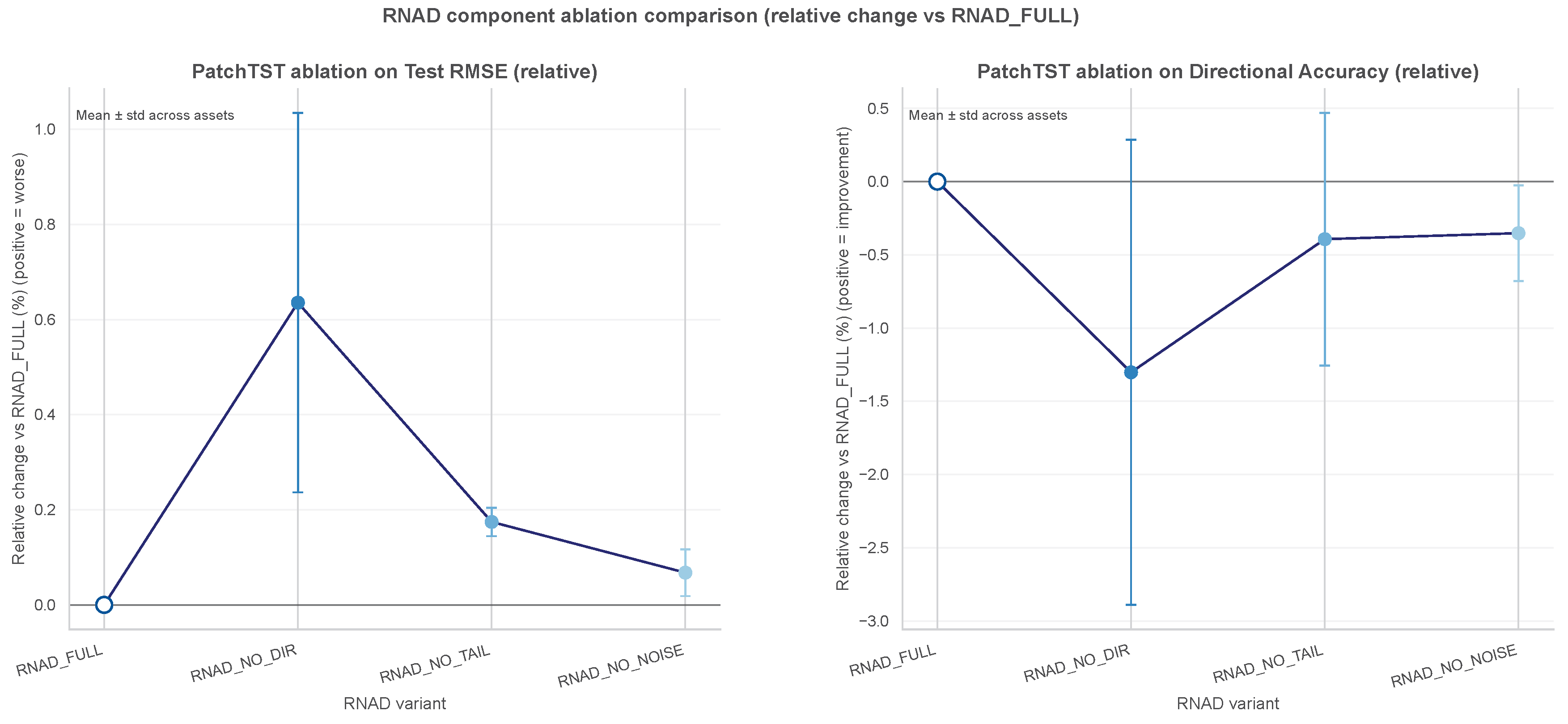
Removing the directional penalty consistently degrades RMSE (mean across the four assets) and reduces DA on three of the four assets. This indicates that directional supervision contributes to both magnitude accuracy and directional accuracy, as discussed in Section 8.2. The effect is largest on BTCUSD (), where economically significant directional returns are most frequent.
Tail gating (NO TAIL).
The contribution of tail gating is asset-dependent. On BTCUSD, removing the tail gate yields a marginal RMSE improvement (), suggesting that transitions slightly too aggressively for BTCUSD’s heavier tails. On AUDUSD, US500, and XAUUSD, the full loss is preferred over NO TAIL. These results indicate that is the parameter most sensitive to asset-specific tail behavior.
Noise gating (NO NOISE).
The effects of noise gating are mixed and generally modest. On AUDUSD and BTCUSD, disabling the gate slightly improves RMSE ( and , respectively) and increases DA. On US500, disabling the gate slightly worsens RMSE () and reduces DA. On XAUUSD, the RMSE change is negligible, but DA decreases by pp. Overall, noise gating functions as a conservative regularizer whose impact is regime-dependent.
Figure 3.
Ablation effects on RMSE and DA. Percentage change in RMSE and DA when each RNAD component is removed from the full objective across four representative assets. Directional supervision has the most consistent effect, while tail gating and noise gating produce smaller, asset-dependent changes.
Figure 3.
Ablation effects on RMSE and DA. Percentage change in RMSE and DA when each RNAD component is removed from the full objective across four representative assets. Directional supervision has the most consistent effect, while tail gating and noise gating produce smaller, asset-dependent changes.
8. Discussion
This section interprets the empirical findings rather than introducing new experiments. It explains why RNAD improves both RMSE and directional accuracy, how the magnitude and directional terms interact, and why the gains vary across backbones and assets. The goal is to connect the observed benchmark behavior back to the optimization geometry described earlier.
8.1. Why RNAD Improves Forecasting
The consistent RMSE improvements on transformer-style backbones are best understood through gradient signal quality. Standard MSE generates parameter updates proportional to raw residual magnitude, conflating forecast residual with volatility scale. In high-volatility regimes, large shocks dominate gradient updates, steering optimization toward minimizing absolute magnitude rather than learning regime-relative structure. In low-volatility periods, directional noise weakens sign gradients. RNAD addresses both pathologies: volatility normalization calibrates gradient magnitude to predictive difficulty, tail gating bounds the influence of extreme events, and gated directional supervision injects sign information that MSE cannot express.
This interpretation is consistent with a higher signal-to-noise ratio in the gradient stream. By normalizing residuals by s, the loss makes gradient magnitudes reflect how unexpected a residual is relative to the prevailing regime rather than how large it is in absolute terms. The directional term then adds asymmetric penalties around the sign boundary, explicitly encoding the economically motivated half-plane constraint that MSE ignores.
8.2. Directional–Magnitude Coupling
An important empirical finding from the ablation study (Table 10) is that removing the directional penalty (NO_DIR) not only reduces directional accuracy but also consistently increases RMSE. This coupling arises from the geometry of the forecast residual: a sign error amplifies the residual magnitude even when the predicted price level is otherwise close to the true level.
Algebraic illustration.
Let be the realised return and the predicted return. The residual can be written as
When the signs of and disagree, the absolute residual is strictly larger than the maximum of and ; in the worst case, where but the signs are opposite, we obtain
Thus, a single sign-error event contributes roughly four times as much to the global MSE as a correct-sign prediction of the same magnitude, even if the price forecast is accurate in absolute terms. By penalising directional mistakes, RNAD explicitly pushes into the correct half-plane, thereby reducing the frequency of these squared-error amplifying events and directly lowering RMSE—even with a modest directional weight .
Empirical verification on BTCUSD.
To verify this coupling, we examine the test-set predictions of RNAD on BTCUSD (the most volatile asset, where the effect is most pronounced). Figure 4 displays the distribution of separated by whether the predicted return sign matched the realised sign. The wrong-sign distribution is markedly shifted toward larger absolute residuals, with a long right tail populated by precisely the type of compounded errors described in Eq. (21). Table 11 reports the corresponding group-level statistics: wrong-sign predictions exhibit an average that is approximately 35% larger than the correct-sign average (326.89 vs. 242.80). This direct empirical decomposition confirms that sign errors are a primary structural source of large residuals, and that improving directional consistency mechanically reduces RMSE.
In summary, the directional penalty in RNAD acts as an implicit constraint that steers predictions away from the sign-error region, thereby stabilising the magnitude component and producing the joint improvement in RMSE and DA observed throughout the benchmark.
8.3. Architectural Interactions
The architecture-dependent benefit pattern—large gains on transformer-family backbones and smaller gains on N-HiTS—supports the interpretation that loss-level and architecture-level regime awareness partially overlap. N-HiTS’s hierarchical decomposition already captures some regime structure; the marginal benefit of RNAD is correspondingly smaller when the backbone has partially addressed the same failure mode. Importantly, RNAD does not degrade backbone-level aggregate RMSE: on N-HiTS the gain is modest but positive ( versus MSE), confirming that the loss is safely composable with regime-aware architectures.
8.4. Statistical Stability
The small standard deviations of RNAD RMSE across seeds ( on transformer backbones; Table 7) confirm that the observed improvements are stable across random initializations. This stability is consistent with the gradient-level explanation above: the gains arise from systematic changes in the optimization geometry rather than favorable sampling of the loss landscape.
9. Limitations
Theoretical foundations.
RNAD is designed on geometric and empirical grounds. No convergence guarantees, Bayes-optimality certificates, or formal proof that the gated directional term constitutes a proper scoring rule (Gneiting & Raftery, 2007) are provided. The EMA volatility estimator introduces first-order autocorrelation in the effective loss landscape and may misrepresent long-memory volatility dynamics not captured by the GARCH-like EMA kernel. Formal Diebold–Mariano or Model Confidence Set tests (Diebold & Mariano, 1995; Hansen et al., 2011) were not applied; extending the benchmark with such comparisons is an important direction for future work.
Hyperparameter sensitivity.
The loss introduces ten scalar controls (Table 5). While the default values are empirically robust to perturbations for most parameters, is the most sensitive control and may merit retuning when transferring to a substantially different market universe. The tail-gating parameters and are moderately sensitive on heavy-tailed assets (see the BTCUSD ablation results in Table 10) and are the most plausible targets for asset-specific calibration.
Scope of demonstrated improvements.
Consistent gains are concentrated in one-step-ahead, raw-price prediction on attention-based architectures. Benefits are weaker or absent on regime-aware architectures, at longer forecasting horizons, and in return-domain or log-price formulations where normalization is less critical. Practitioners should validate RNAD on their own setup before assuming transferability.
Economic validity of directional accuracy.
The DA metric (Eq. 19) weights all non-zero returns equally regardless of magnitude or economic significance, and does not account for transaction costs, bid–ask spread, slippage, position sizing, or the asymmetric utility of large versus small directional errors. Higher DA does not imply higher risk-adjusted returns, and this study makes no such claim. Evaluation within a full trading simulation with realistic costs is necessary to draw conclusions about practical financial value.
Statefulness and engineering overhead.
The EMA buffer must be synchronized across data-parallel workers, persisted at checkpoints, and reset at each training initialization. This engineering overhead is absent in stateless losses and may complicate deployment in distributed training pipelines.
Batch dependence.
Because the volatility scale and gates are computed from mini-batches, the objective is mildly batch-size dependent; smaller batches yield noisier scale estimates and can alter the effective gate values. Batch size is held fixed at 64 in all experiments, which controls but does not eliminate this effect.
Evaluation breadth.
The benchmark uses three seeds and a single chronological split per asset. Extending to multiple non-overlapping temporal windows and applying bootstrap inference over test-set samples would substantially strengthen the statistical conclusions.
10. Conclusion
We introduced RNAD, a regime-normalized adaptive directional loss for financial time-series forecasting. By combining adaptive volatility normalization, tail-robust magnitude handling, and gated directional learning within a single differentiable objective, RNAD aligns the training geometry with the distinctive statistical structure of financial markets: regime-switching, heavy-tailed, and sign-sensitive.
Comprehensive benchmarks across nine assets and four architectures demonstrate consistent RMSE improvements on transformer-style backbones and the lowest per-asset RMSE under PatchTST for every asset. Controlled ablation studies indicate that all three components contribute independently: directional learning is the primary driver of magnitude improvement; tail gating is most critical on heavy-tailed assets; and noise gating contributes modest, regime-dependent regularization. The loss is computationally lightweight, architecture-agnostic, and requires no modification to model structure, data pipelines, or inference code.
The broader implication is that loss-level design is an important lever for financial forecasting improvement, with effects in this benchmark that are of a comparable order of magnitude to several architectural choices while remaining less costly to deploy. Directional accuracy should be interpreted as a forecast-quality metric rather than a direct proxy for trading profitability; this study does not evaluate transaction costs, slippage, or profit and loss. When the forecasting target is volatile, heavy-tailed, and direction-sensitive—as financial prices characteristically are—the training objective can be highly consequential relative to the choice of model architecture.
Data and Code Availability
The implementation code and configuration files required to reproduce the experiments in this manuscript are publicly available at the following GitHub repository: https://github.com/NabeelAhmadSaidd/RNAD Processed data artifacts are not publicly available because of proprietary or ethical restrictions. They are available from the corresponding author on reasonable request and subject to a signed data use agreement.
Conflicts of Interest
The author declares that there are no conflicts of interest, financial or otherwise, that could have influenced the research, authorship, or publication of this work.
A. Supplementary Diagnostics
This appendix provides supporting analyses that complement the main benchmark tables. It includes visualizations of the loss landscape and gradients, volatility-stratified performance, seed stability summaries, a fuller ablation view, and a brief note on computational overhead. These diagnostics are intended to reinforce the main narrative without interrupting the flow of the main text.
A.1. Loss Landscape and Gradient Dynamics
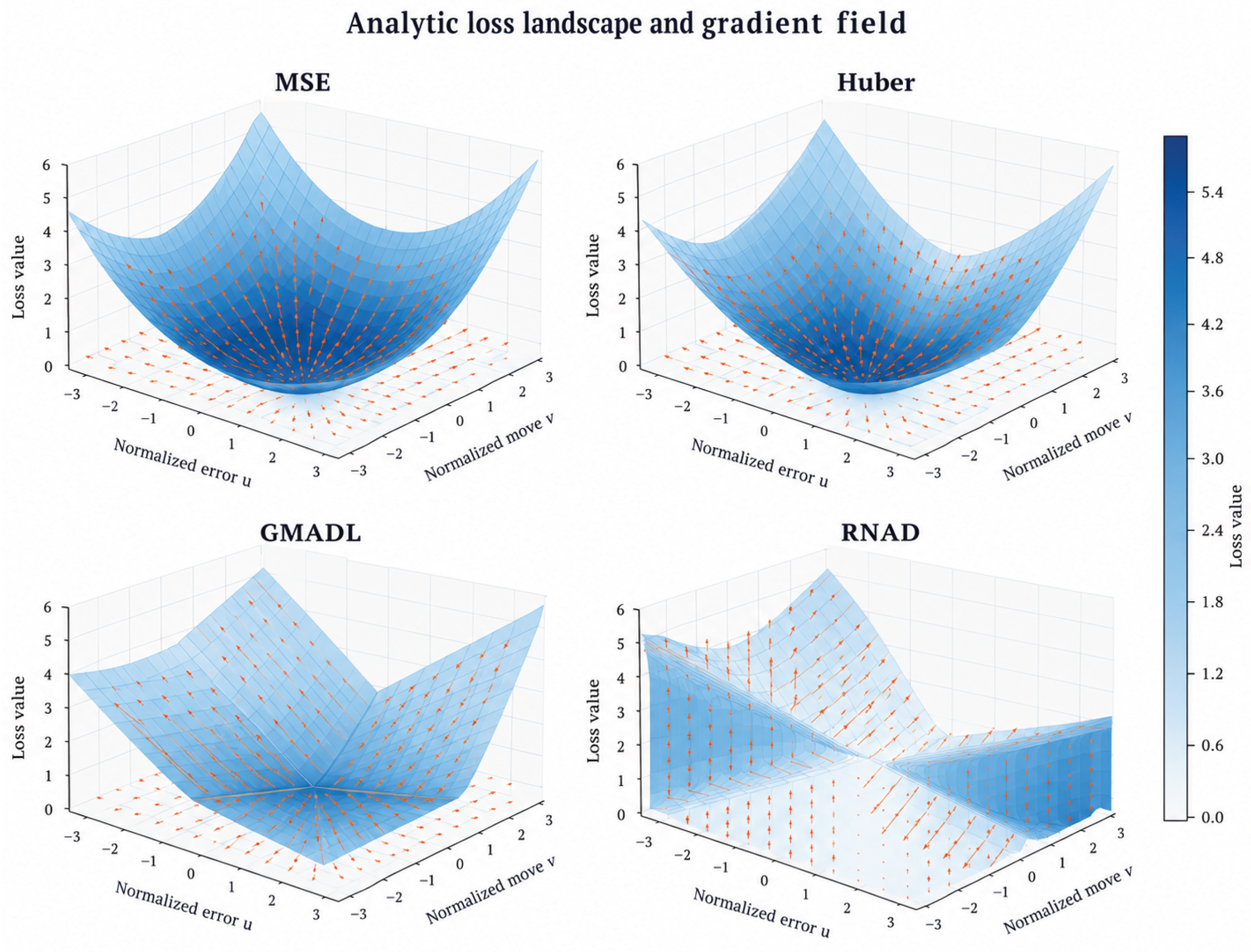
Figure 5 contrasts the gradient vector fields of MSE, Huber, GMADL, and RNAD as functions of normalized error and realized return . MSE produces gradients that grow linearly with error magnitude and therefore systematically over-weight tail observations in parameter updates. Huber retains MSE-like quadratic behavior near the origin but transitions to linear tails, bounding gradient norms for large residuals. GMADL and RNAD introduce smooth nonlinear damping in the tails: GMADL provides a robust, smoothly saturated gradient response, while RNAD maintains steep, informative gradients near the origin—facilitating precise level learning—and transitions to sub-linear damping during extreme events. Across the four losses, the comparison separates unbounded quadratic sensitivity (MSE), piecewise linear tail control (Huber), and smooth nonlinear tail damping (GMADL and RNAD).
Figure 5.
Gradient-field comparison of MSE, Huber, GMADL, and RNAD. MSE gradients grow linearly without bound; Huber uses quadratic small-error and linear tail gradients; GMADL and RNAD apply smooth nonlinear damping to extreme residuals while preserving informative gradients near small errors.
Figure 5.
Gradient-field comparison of MSE, Huber, GMADL, and RNAD. MSE gradients grow linearly without bound; Huber uses quadratic small-error and linear tail gradients; GMADL and RNAD apply smooth nonlinear damping to extreme residuals while preserving informative gradients near small errors.
A.2. Regime-Stratified Performance
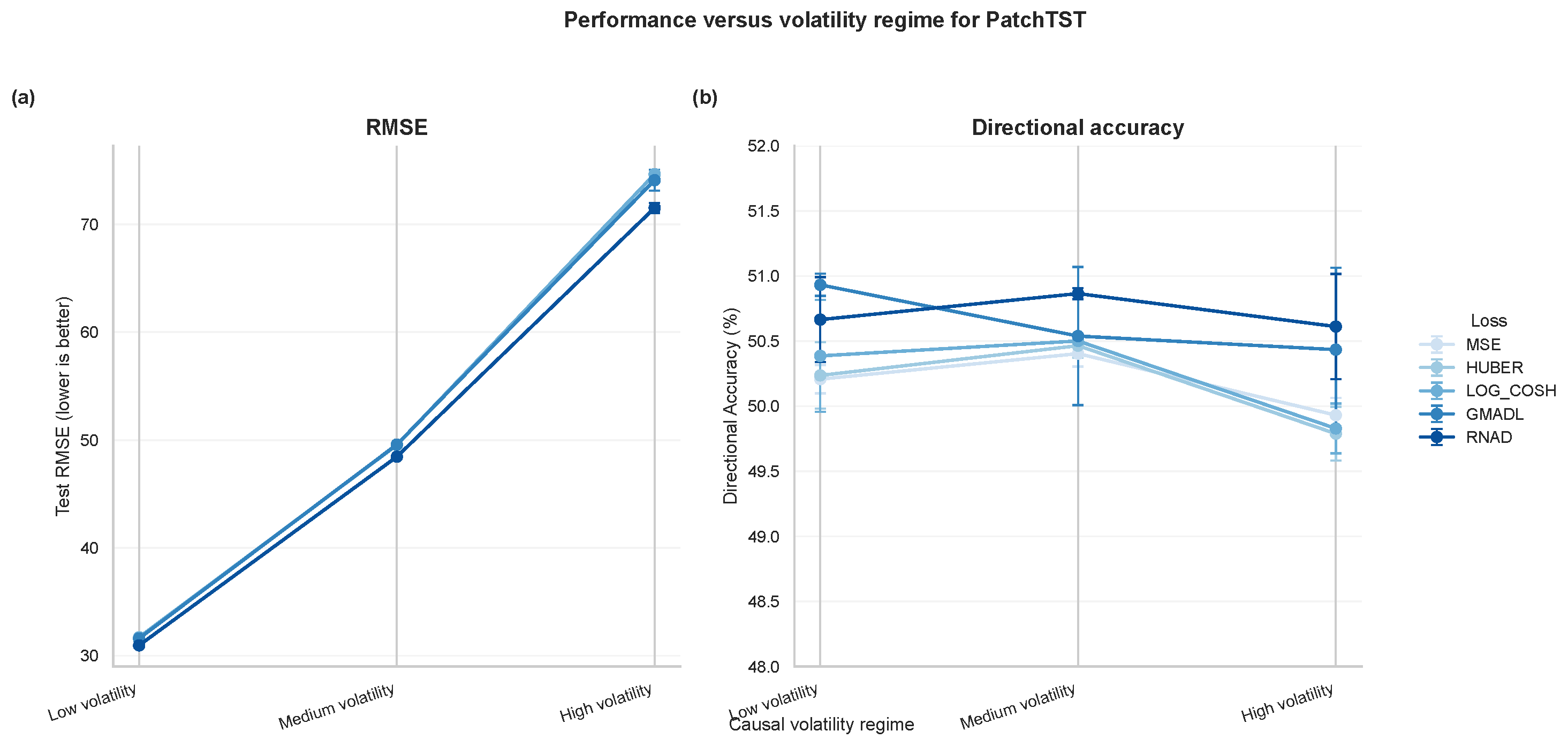
Figure 6 stratifies test performance by causal volatility regime (terciles of realized volatility computed from training-set statistics, to avoid look-ahead bias). RNAD maintains a consistent performance advantage over MSE across all three regimes, indicating that adaptive normalization generalizes across volatility levels rather than simply exploiting tail events.
Figure 6.
Performance across volatility regimes. RMSE and DA are shown for BTCUSD, US500, and XAUUSD under low-, medium-, and high-volatility terciles. RNAD retains its advantage over MSE across regimes, indicating that the gain is not confined to a single volatility band.
Figure 6.
Performance across volatility regimes. RMSE and DA are shown for BTCUSD, US500, and XAUUSD under low-, medium-, and high-volatility terciles. RNAD retains its advantage over MSE across regimes, indicating that the gain is not confined to a single volatility band.
A.3. Seed Stability
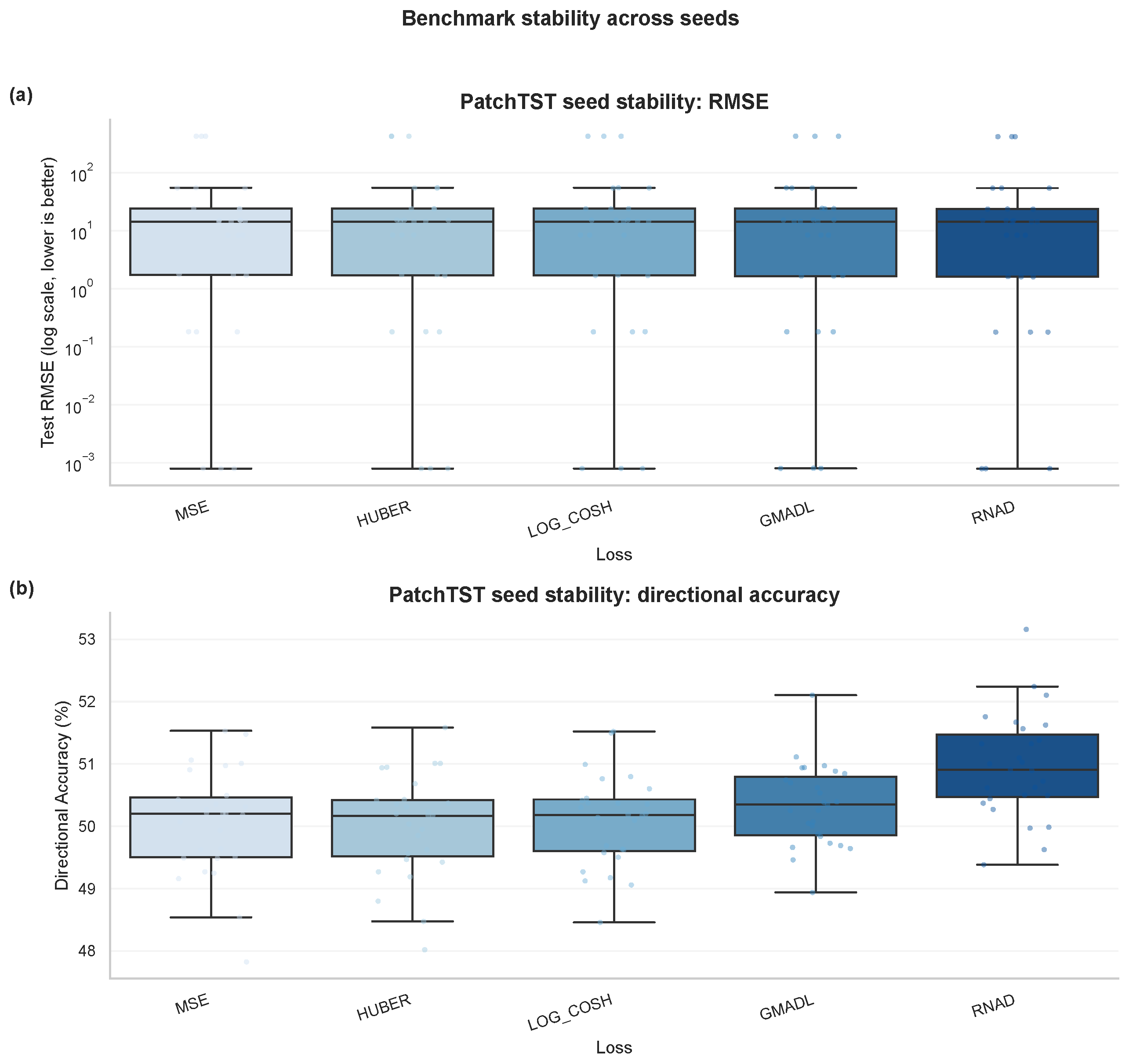
Figure 7 shows box-and-whisker distributions of RMSE and DA across nine assets and three seeds. RNAD distributions are consistently shifted toward lower error, with narrow whiskers indicating that improvements arise from the loss geometry rather than favorable initialization.
Figure 7.
Seed stability across nine assets. The boxplots summarize PatchTST test RMSE on a log scale and directional accuracy over three random seeds for each loss, showing that RNAD shifts performance toward lower error and higher sign consistency.
Figure 7.
Seed stability across nine assets. The boxplots summarize PatchTST test RMSE on a log scale and directional accuracy over three random seeds for each loss, showing that RNAD shifts performance toward lower error and higher sign consistency.
A.4. Full Ablation: All Assets and Components
Figure 8.
Per-asset RMSE change under ablation. The plot shows the change in RMSE relative to the full RNAD loss for each ablation variant on the reported assets, indicating that removing any component is consistently non-beneficial.
Figure 8.
Per-asset RMSE change under ablation. The plot shows the change in RMSE relative to the full RNAD loss for each ablation variant on the reported assets, indicating that removing any component is consistently non-beneficial.
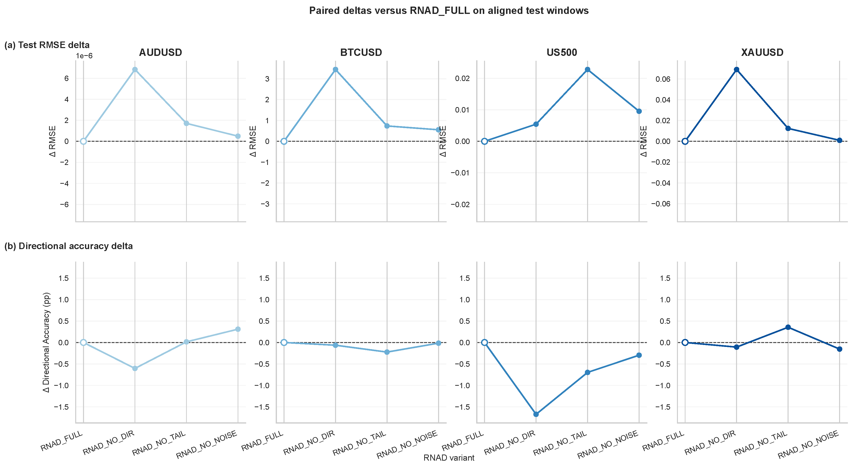
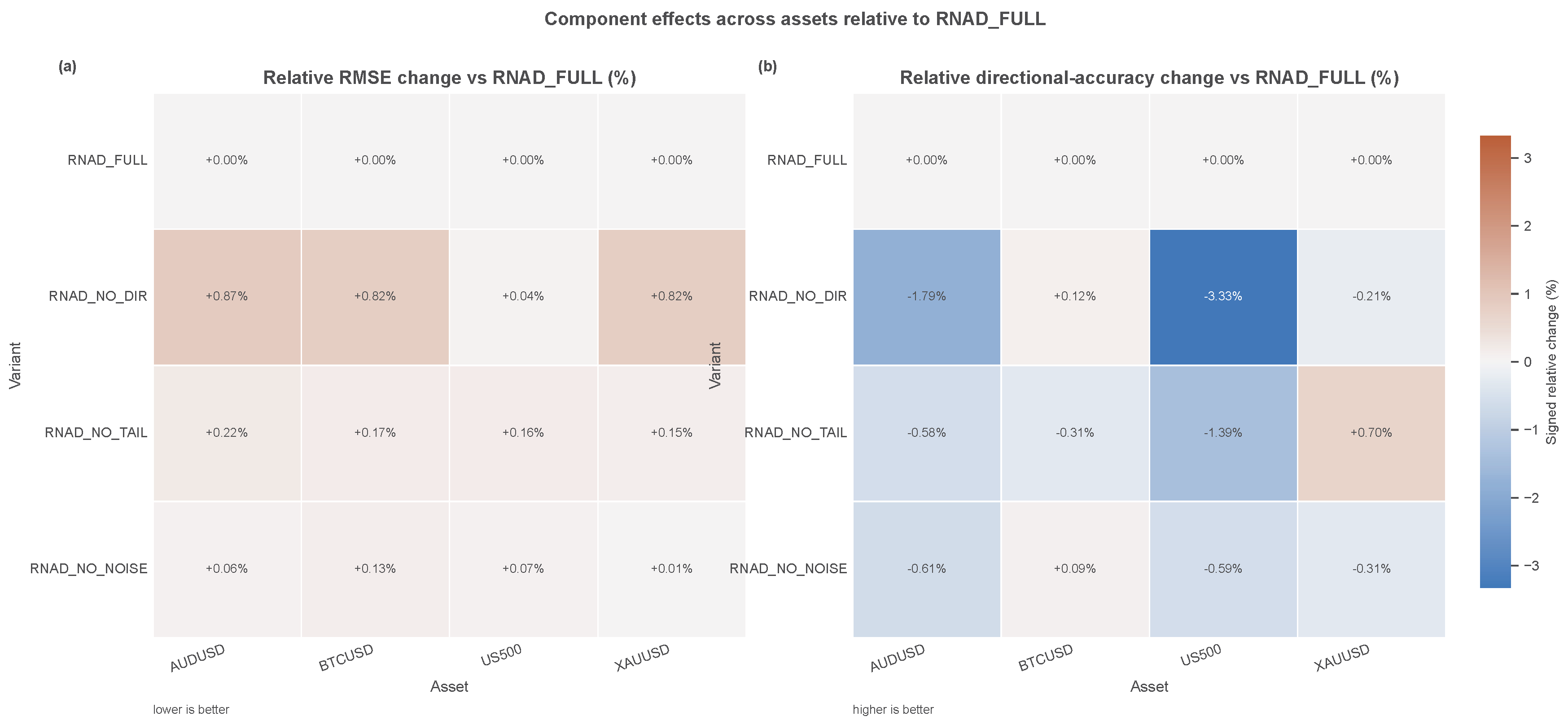
Figure 9.
Component contribution heatmap. Mean RMSE increases from ablating each RNAD component are shown by asset and component, with darker cells indicating greater reliance on that component. The directional term is the most consistent contributor, while tail gating matters most for the most volatile assets.
Figure 9.
Component contribution heatmap. Mean RMSE increases from ablating each RNAD component are shown by asset and component, with darker cells indicating greater reliance on that component. The directional term is the most consistent contributor, while tail gating matters most for the most volatile assets.
A.5. Computational Overhead
RNAD introduces negligible runtime cost relative to MSE. The EMA update (Eq. 5) requires a single scalar multiply-add per gradient step. Additional loss computations—tanh, logistic gate, softplus—are elementwise operations parallelized by the autograd engine with no synchronization barrier. Memory overhead amounts to one floating-point scalar per asset. In wall-clock benchmarks on all four backbones, training and inference throughput are indistinguishable from MSE at standard batch sizes.
Table 12.
Per-epoch training time and peak GPU memory for RNAD compared with MSE, measured on BTCUSD (seed 178, batch size 64) under the exact benchmark configuration. The total wall-clock time for the full 50-epoch training budget is approximated by multiplying the epoch time by 50 (validation overhead is negligible).
Table 12.
Per-epoch training time and peak GPU memory for RNAD compared with MSE, measured on BTCUSD (seed 178, batch size 64) under the exact benchmark configuration. The total wall-clock time for the full 50-epoch training budget is approximated by multiplying the epoch time by 50 (validation overhead is negligible).
| Backbone | Loss | Time per epoch (s) | Peak GPU memory (MiB) | Est. total time (h) |
|---|---|---|---|---|
| PatchTST | MSE | 12.17 | 63.3 | 0.169 |
| RNAD | 13.38 | 63.3 | 0.186 | |
| iTransformer | MSE | 11.47 | 50.4 | 0.159 |
| RNAD | 12.16 | 50.4 | 0.169 | |
| N-HiTS | MSE | 8.20 | 26.7 | 0.114 |
| RNAD | 9.03 | 26.7 | 0.125 | |
| TimeXer | MSE | 12.93 | 34.4 | 0.180 |
| RNAD | 13.91 | 34.4 | 0.193 |
Note: The RNAD overhead consists of a few element-wise operations (EMA update, tanh, sigmoids, softplus) fully parallelised on the GPU, resulting in a negligible increase in runtime and no measurable increase in peak memory.
References
- Barron, J. T. (2019). A general and adaptive robust loss function. In Ieee/cvf conference on computer vision and pattern recognition (cvpr) (pp. 4331–4339). [CrossRef]
- Bollerslev, T. (1986). Generalized autoregressive conditional heteroskedasticity. Journal of Econometrics, 31(3), 307–327. [CrossRef]
- Challu, C., Olivares, K. G., Oreshkin, B. N., Garza, F., Mergenthaler-Canseco, M., & Dubrawski, A. (2023). N-HiTS: Neural hierarchical interpolation for time series forecasting. In Proceedings of aaai (Vol. 37, pp. 6989–6997). [CrossRef]
- Charbonnier, P., Blanc-Féraud, L., Aubert, G., & Barlaud, M. (1997). Deterministic edge-preserving regularization in computed imaging. IEEE Transactions on Image Processing, 6(2), 298–311. [CrossRef]
- Clark, T. E., & West, K. D. (2007). Approximately normal tests for equal predictive accuracy in nested models. Journal of Econometrics, 138(1), 291–311. [CrossRef]
- Cont, R. (2001). Empirical properties of asset returns: Stylized facts and statistical issues. Quantitative Finance, 1(2), 223–236. [CrossRef]
- Diebold, F. X., & Mariano, R. S. (1995). Comparing predictive accuracy. Journal of Business & Economic Statistics, 13(3), 253–263. [CrossRef]
- Engle, R. F. (1982). Autoregressive conditional heteroskedasticity with estimates of the variance of United Kingdom inflation. Econometrica, 50(4), 987–1007. [CrossRef]
- Fan, W., Wang, S., Wang, Y., Wang, X., Zhao, H., Liu, T., Shen, C., Xu, Q., Liu, G., & Wang, X. (2023). Dish-TS: A general paradigm for alleviating distribution shift in time series forecasting. In Proceedings of aaai (Vol. 37, pp. 7522–7529). [CrossRef]
- Gneiting, T., & Raftery, A. E. (2007). Strictly proper scoring rules, prediction, and estimation. Journal of the American Statistical Association, 102(477), 359–378. [CrossRef]
- Hamilton, J. D. (1989). A new approach to the economic analysis of nonstationary time series and the business cycle. Econometrica, 57(2), 357–384. [CrossRef]
- Hansen, P. R., Lunde, A., & Nason, J. M. (2011). The model confidence set. Econometrica, 79(2), 453–497. [CrossRef]
- Huber, P. J. (1964). Robust estimation of a location parameter. The Annals of Mathematical Statistics, 35(1), 73–101. [CrossRef]
- Kendall, A., Gal, Y., & Cipolla, R. (2018). Multi-task learning using uncertainty to weigh losses for scene geometry and semantics. In Ieee/cvf conference on computer vision and pattern recognition (cvpr) (pp. 7482–7491). [CrossRef]
- Kim, T., Kim, J., Tae, Y., Park, C., Choi, J.-H., & Choo, J. (2022). Reversible Instance Normalization for Accurate Time-Series Forecasting against Distribution Shift. In The tenth international conference on learning representations (iclr).
- Koenker, R., & Bassett, G. (1978). Regression quantiles. Econometrica, 46(1), 33–50. [CrossRef]
- Leitch, G., & Tanner, J. E. (1991). Economic forecast evaluation: Profits versus the conventional error measures. American Economic Review, 81(3), 580–590.
- Liu, Y., Hu, T., Zhang, H., Wu, H., Wang, S., Ma, L., & Long, M. (2024). iTransformer: Inverted Transformers Are Effective for Time Series Forecasting. In The twelfth international conference on learning representations (iclr). [CrossRef]
- Makridakis, S., Spiliotis, E., & Assimakopoulos, V. (2022). M5 accuracy competition: Results, findings, and conclusions. International Journal of Forecasting, 38(4), 1346–1364. [CrossRef]
- Mandelbrot, B. B. (1963). The variation of certain speculative prices. The Journal of Business, 36(4), 394–419. [CrossRef]
- Michańków, J., Sakowski, P., & Ślepaczuk, R. (2024). Generalized mean absolute directional loss as a solution to overfitting and high transaction costs in machine learning models used in high-frequency algorithmic investment strategies. (arXiv preprint arXiv:2412.18405). [CrossRef]
- Nie, Y., Nguyen, N. H., Sinthong, P., & Kalagnanam, J. (2023). A Time Series is Worth 64 Words: Long-term Forecasting with Transformers. In The eleventh international conference on learning representations (iclr). [CrossRef]
- Oreshkin, B. N., Carpov, D., Chapados, N., & Bengio, Y. (2020). N-BEATS: Neural Basis Expansion Analysis for Interpretable Time Series Forecasting. In The eighth international conference on learning representations (iclr). [CrossRef]
- Pesaran, M. H., & Timmermann, A. (1992). A simple nonparametric test of predictive performance. Journal of Business & Economic Statistics, 10(4), 461–465. [CrossRef]
- Saidd, N. A. (2026a). A controlled comparison of deep learning architectures for multi-horizon financial forecasting: Evidence from 918 experiments. [CrossRef]
- Saidd, N. A. (2026b). RADIAN: Regime-Adaptive Dilated Inter-Attention Network for Non-Stationary Financial Time-Series Forecasting. Preprints.org. [CrossRef]
- Saleh, R. A., & Saleh, A. K. M. E. (2022). Statistical properties of the log-cosh loss function used in machine learning. [CrossRef]
- Salinas, D., Flunkert, V., Gasthaus, J., & Januschowski, T. (2020). DeepAR: Probabilistic forecasting with autoregressive recurrent networks. International Journal of Forecasting, 36(3), 1181–1191. [CrossRef]
- van den Oord, A., Dieleman, S., Zen, H., Simonyan, K., Vinyals, O., Graves, A., Kalchbrenner, N., Senior, A., & Kavukcuoglu, K. (2016). Wavenet: A generative model for raw audio. [CrossRef]
- Vaswani, A., Shazeer, N., Parmar, N., Uszkoreit, J., Jones, L., Gomez, A. N., Kaiser, L., & Polosukhin, I. (2017). Attention Is All You Need. In Advances in neural information processing systems (Vol. 30, pp. 5998–6008). Curran Associates, Inc. [CrossRef]
- Wang, Y., Wu, H., Dong, J., Qin, G., Zhang, H., Liu, Y., Qiu, Y., Wang, J., & Long, M. (2024). Timexer: Empowering transformers for time series forecasting with exogenous variables. [CrossRef]
- Zeng, A., Chen, M., Zhang, L., & Xu, Q. (2023). Are transformers effective for time series forecasting? In Proceedings of aaai (Vol. 37, pp. 11121–11128). [CrossRef]
Figure 1.
Schematic of the RNAD loss architecture. The diagram illustrates EMA-based volatility estimation and normalization, followed by two parallel loss branches. The tail-adaptive magnitude branch smoothly blends an L2 penalty with a Charbonnier-style robust penalty according to the normalized error magnitude. The noise-aware directional branch uses a smooth gate based on the true normalized change to weight the directional penalty. The two components are combined into the total objective, with the directional loss scaled by . The EMA state is updated during training and remains unchanged during evaluation.
Figure 1.
Schematic of the RNAD loss architecture. The diagram illustrates EMA-based volatility estimation and normalization, followed by two parallel loss branches. The tail-adaptive magnitude branch smoothly blends an L2 penalty with a Charbonnier-style robust penalty according to the normalized error magnitude. The noise-aware directional branch uses a smooth gate based on the true normalized change to weight the directional penalty. The two components are combined into the total objective, with the directional loss scaled by . The EMA state is updated during training and remains unchanged during evaluation.
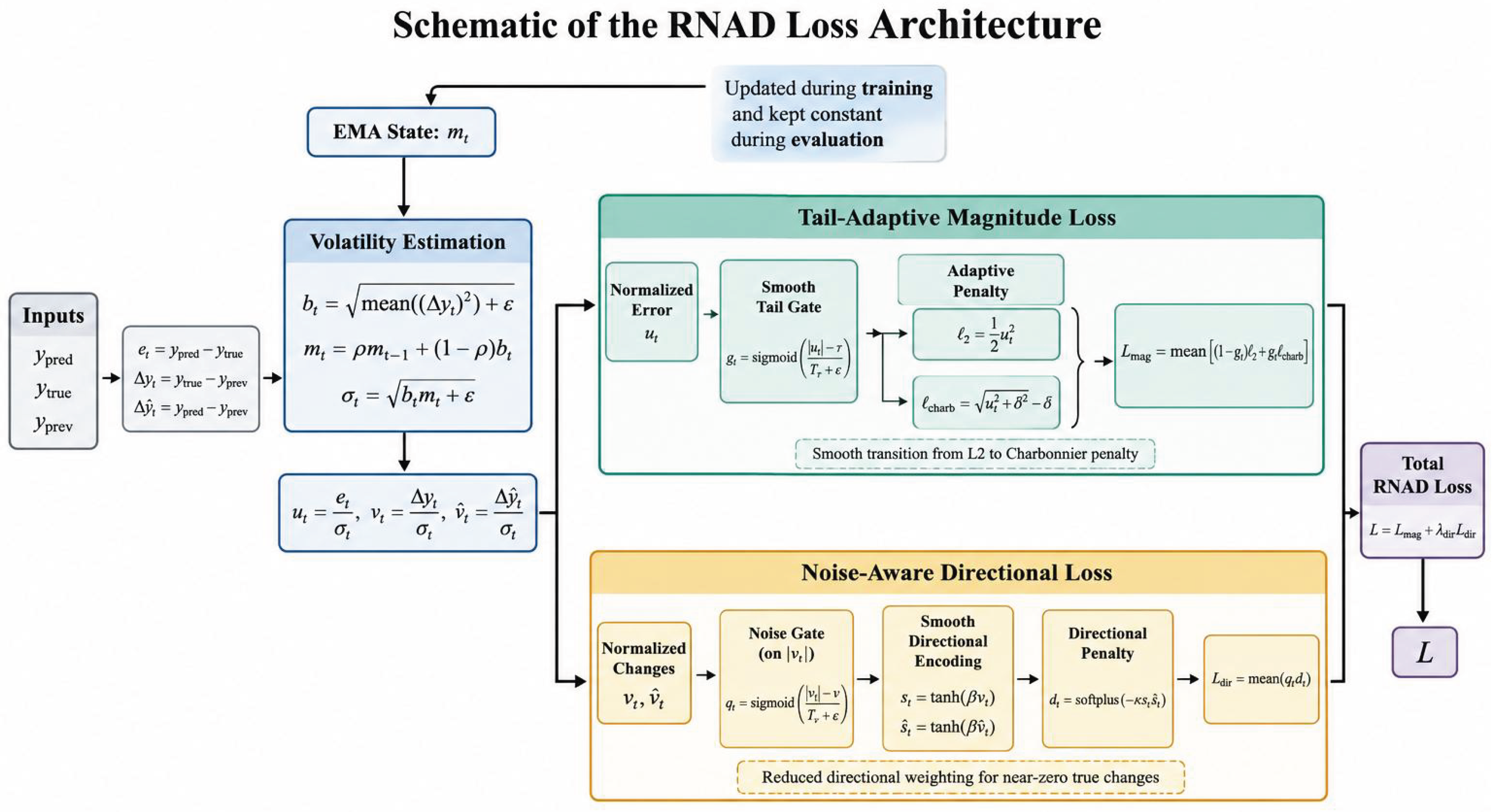
Figure 2.
RNAD loss surface. The surface combines a quadratic basin for small errors, robust tail flattening for large residuals, and directional penalties when predicted and realized signs disagree.
Figure 2.
RNAD loss surface. The surface combines a quadratic basin for small errors, robust tail flattening for large residuals, and directional penalties when predicted and realized signs disagree.
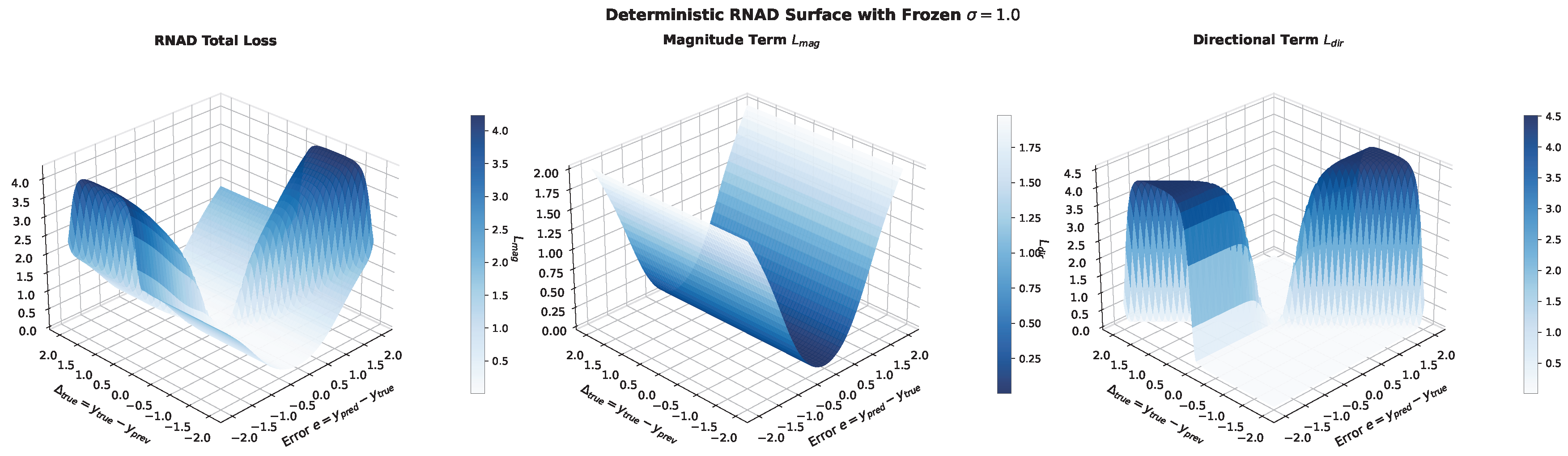
Figure 4.
Distribution of absolute residuals by sign correctness (BTCUSD, test set, RNAD). The density plot separates predictions into correct-sign (green) and wrong-sign (red) groups. The wrong-sign distribution is systematically shifted toward larger and displays a heavy right tail, providing direct empirical evidence for the directional–magnitude coupling mechanism analysed in Eq. (21).
Figure 4.
Distribution of absolute residuals by sign correctness (BTCUSD, test set, RNAD). The density plot separates predictions into correct-sign (green) and wrong-sign (red) groups. The wrong-sign distribution is systematically shifted toward larger and displays a heavy right tail, providing direct empirical evidence for the directional–magnitude coupling mechanism analysed in Eq. (21).
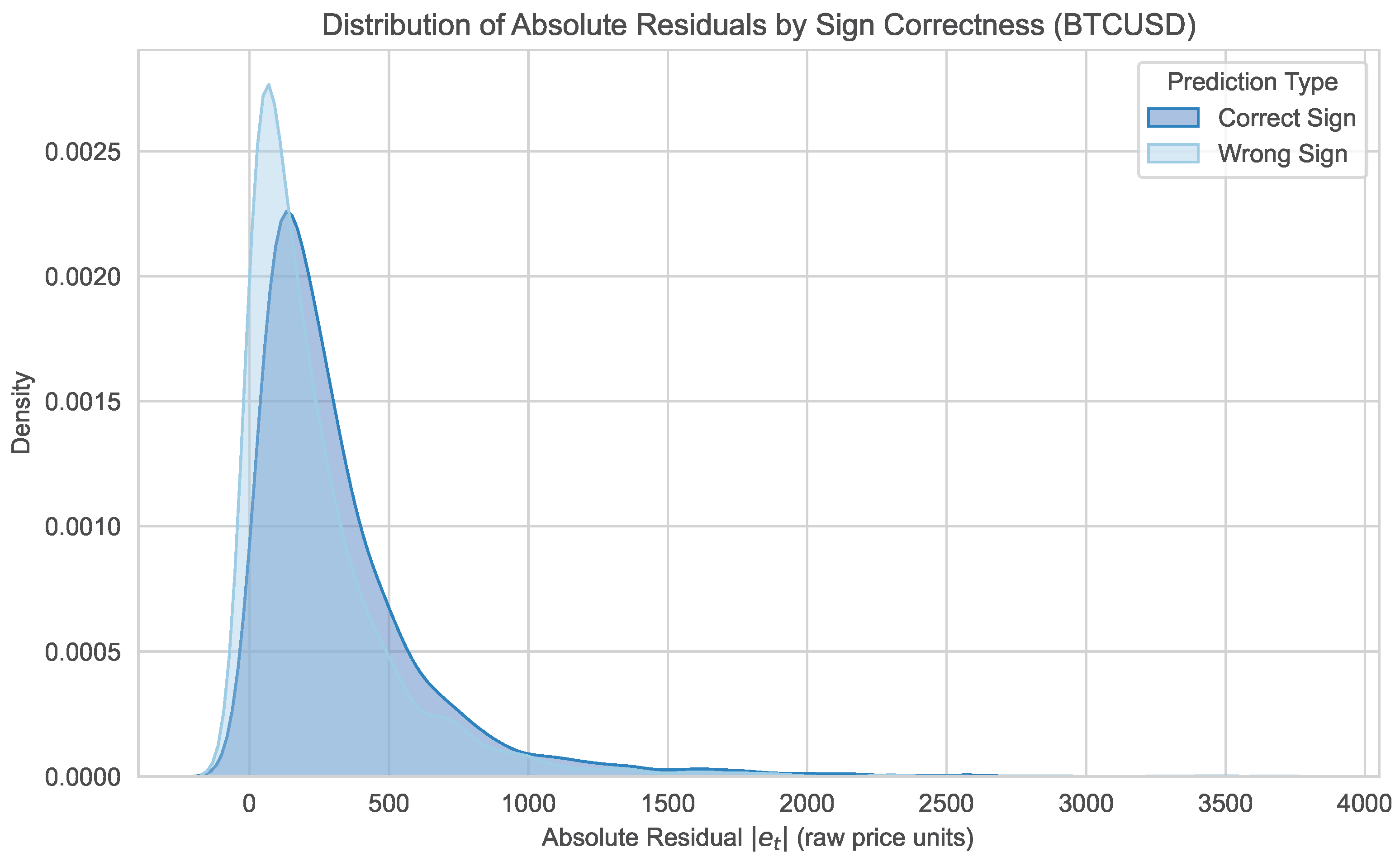
Table 1.
Summary of the nine assets used in the benchmark. All series share the same OHLCV-plus-indicator feature set, a close-price target, and an chronological split; the volatility proxy is the training-set RMS return used to initialize the EMA state.
Table 1.
Summary of the nine assets used in the benchmark. All series share the same OHLCV-plus-indicator feature set, a close-price target, and an chronological split; the volatility proxy is the training-set RMS return used to initialize the EMA state.
| Asset | Market Type | Total | Train | Val | Test | Vol. Proxy |
|---|---|---|---|---|---|---|
| AAPL | Equity | 15,673 | 12,538 | 1,567 | 1,568 | 0.00616 |
| AUDUSD | Forex | 68,535 | 54,828 | 6,853 | 6,854 | 0.00127 |
| BTCUSD | Crypto | 62,793 | 50,234 | 6,279 | 6,280 | 0.00653 |
| DAX30 | Equity Index | 57,783 | 46,226 | 5,778 | 5,779 | 0.00233 |
| ETHUSD | Crypto | 62,783 | 50,226 | 6,278 | 6,279 | 0.00847 |
| FTSE100 | Equity Index | 56,767 | 45,413 | 5,676 | 5,678 | 0.00197 |
| US500 | Equity Index | 57,665 | 46,132 | 5,766 | 5,767 | 0.00200 |
| USDJPY | Forex | 68,536 | 54,828 | 6,853 | 6,855 | 0.00096 |
| XAUUSD | Commodity | 65,093 | 52,074 | 6,509 | 6,510 | 0.00164 |
Table 2.
Configuration summary for the four forecasting backbones. The table lists the main architecture settings and the retained implementation options used in the benchmark.
Table 2.
Configuration summary for the four forecasting backbones. The table lists the main architecture settings and the retained implementation options used in the benchmark.
| Backbone | Exact configuration | Additional settings |
|---|---|---|
| PatchTST | 3 encoder layers; 4 attention heads; ; ; patch length ; stride ; dropout ; fc-dropout ; head-dropout | RevIN enabled; series decomposition disabled; BatchNorm backbone; GELU activation; individual=false; res_attention=true; pe=zeros; learn_pe=true |
| iTransformer | 3 encoder layers; 8 attention heads; ; ; dropout ; GELU activation | Inverted linear embedding over the 24-step input window; LayerNorm encoder; attention factor ; target index |
| N-HiTS | 3 stacks; 2 blocks per stack; 2 MLP layers per block; ; dropout | Max pooling; kernel sizes ; downsampling rates ; linear interpolation; ReLU activation; batch normalization disabled; shared weights disabled |
| TimeXer | 2 encoder layers; 8 attention heads; ; ; patch length ; dropout ; attention factor | Three non-overlapping target patches over ; global token enabled; use_norm=true; GELU activation |
Table 6.
Main benchmark comparison across four backbones, five losses, nine assets, and three seeds (). Lower RMSE and MAE are better, higher DA (%) is better, and RMSE reports RNAD’s improvement over the strongest non-RNAD baseline within each backbone. Bold and underlining mark the best and second-best values.
Table 6.
Main benchmark comparison across four backbones, five losses, nine assets, and three seeds (). Lower RMSE and MAE are better, higher DA (%) is better, and RMSE reports RNAD’s improvement over the strongest non-RNAD baseline within each backbone. Bold and underlining mark the best and second-best values.
| Backbone | Loss | RMSE | MAE | DA (%) | RMSE |
|---|---|---|---|---|---|
| PatchTST | MSE | ||||
| Huber | |||||
| log-cosh | |||||
| GMADL | |||||
| RNAD | |||||
| iTransformer | MSE | ||||
| Huber | |||||
| log-cosh | |||||
| GMADL | |||||
| RNAD | |||||
| N-HiTS | MSE | ||||
| Huber | |||||
| log-cosh | |||||
| GMADL | |||||
| RNAD | |||||
| TimeXer | MSE | ||||
| Huber | |||||
| log-cosh | |||||
| GMADL | |||||
| RNAD |
Table 7.
Backbone-level averages of RMSE and DA across nine assets and three seeds. The columns report RNAD’s RMSE improvement relative to MSE and GMADL, and the final column identifies the best loss for each backbone.
Table 7.
Backbone-level averages of RMSE and DA across nine assets and three seeds. The columns report RNAD’s RMSE improvement relative to MSE and GMADL, and the final column identifies the best loss for each backbone.
| Backbone | Avg RMSE | Avg DA | vs. MSE | vs. GMADL | Best Loss |
|---|---|---|---|---|---|
| PatchTST | 50.29 | RNAD | |||
| iTransformer | 61.18 | RNAD | |||
| N-HiTS | 61.08 | 50.16 | RNAD | ||
| TimeXer | RNAD |
Table 9.
Multi-step () forecasting performance of PatchTST with RNAD and MSE on US500 and USDJPY (seed 178).
Table 9.
Multi-step () forecasting performance of PatchTST with RNAD and MSE on US500 and USDJPY (seed 178).
| Dataset | Loss | RMSE per step | DA per step (%) | RMSEflat | DAavg (%) | ||||||
|---|---|---|---|---|---|---|---|---|---|---|---|
| US500 | RNAD | 14.341 | 19.966 | 24.431 | 28.315 | 51.27 | 51.68 | 52.82 | 52.32 | 22.377 | 52.02 |
| MSE | 14.504 | 20.088 | 24.459 | 28.343 | 49.53 | 49.36 | 50.11 | 49.53 | 22.447 | 49.63 | |
| USDJPY | RNAD | 0.180 | 0.256 | 0.315 | 0.367 | 50.38 | 51.45 | 51.92 | 50.45 | 0.288 | 51.05 |
| MSE | 0.184 | 0.258 | 0.317 | 0.368 | 49.43 | 48.91 | 50.54 | 49.67 | 0.290 | 49.64 | |
Note: RMSE values are given on the raw price scale and rounded to three decimal places; DA (directional accuracy, %) is rounded to two decimal places. RMSEflat is computed over the flattened test samples; DAavg is the arithmetic mean of the four per-step directional accuracies.
Table 11.
Average absolute residual grouped by directional correctness for RNAD on BTCUSD (test set). The wrong-sign group displays a substantially larger mean, consistent with the algebraic doubling effect discussed in the text.
Table 11.
Average absolute residual grouped by directional correctness for RNAD on BTCUSD (test set). The wrong-sign group displays a substantially larger mean, consistent with the algebraic doubling effect discussed in the text.
| Prediction Type | Count | Mean |
|---|---|---|
| Correct-Sign Predictions | 3162 | 242.80 |
| Wrong-Sign Predictions | 3088 | 326.89 |
Disclaimer/Publisher’s Note: The statements, opinions and data contained in all publications are solely those of the individual author(s) and contributor(s) and not of MDPI and/or the editor(s). MDPI and/or the editor(s) disclaim responsibility for any injury to people or property resulting from any ideas, methods, instructions or products referred to in the content. |
© 2026 by the authors. Licensee MDPI, Basel, Switzerland. This article is an open access article distributed under the terms and conditions of the Creative Commons Attribution (CC BY) license (http://creativecommons.org/licenses/by/4.0/).
Copyright: This open access article is published under a Creative Commons CC BY 4.0 license, which permit the free download, distribution, and reuse, provided that the author and preprint are cited in any reuse.