

Submitted:
30 October 2026
Posted:
03 November 2026
You are already at the latest version
Abstract
Field-level crop yield prediction is an important application of precision agriculture, but it remains challenging in African smallholder systems because plots are small, management is heterogeneous, and satellite pixels can mix multiple land covers. This study evaluated machine-learning approaches for predicting maize yield from 6,016 field-year observations in Kenya during 2017–2020 using Sentinel-2 remote-sensing variables, climate, soil, terrain and location attributes, survey-based management information, and 64-dimensional satellite embeddings. Eleven candidate algorithms were compared using cross-validation, followed by XGBoost predictor-group and SHAP analyses. XGBoost achieved the strongest pooled performance (R² = 0.383; RMSE = 1,334 kg ha⁻¹; MAE = 1,013 kg ha⁻¹). Conventional remote sensing alone achieved R² = 0.196; adding climate, soil, terrain, and location increased R² to 0.250, while adding management information increased it to 0.386. Management accounted for 32.4% of grouped SHAP importance, with plant density as the most influential individual predictor. Satellite embeddings matched the predictive performance of conventional remote-sensing predictors while reducing satellite predictor dimensionality by approximately 77%. The results show that remote sensing and machine learning can support field-level yield monitoring in heterogeneous smallholder systems, but plot-level management information remains critical for improving prediction.
Keywords:
precision agriculture
; crop yield prediction
; remote sensing
; machine learning
; Sentinel-2
; satellite embeddings
; smallholder agriculture
; XGBoost
1. Introduction
Timely and spatially detailed information on crop distribution and productivity is fundamental to agricultural planning and food-security assessment. Information on where crops are grown is needed to estimate cultivated areas and monitor changes in land use, while field- and regional-level yield estimates are required to quantify production, identify yield gaps, anticipate supply shortages, and evaluate the effects of agricultural investments and climate variability. Reliable yield information can also support decisions concerning input allocation, extension services, crop insurance, market planning, and the targeting of interventions to areas with persistently low productivity. These needs are particularly important for maize in sub-Saharan Africa, where production is dominated by smallholder systems and where substantial variation in crop performance may occur over relatively short distances.
Conventional estimates of crop production and yield are generally derived from agricultural censuses, household or farm surveys, farmer-reported harvests, crop-cutting exercises, and administrative statistics. These approaches remain indispensable because they provide information that cannot be directly observed from satellites, including crop management, input use, seed choice, labor, and farmer characteristics. However, collecting accurate agricultural survey data requires careful questionnaire design, appropriate timing of survey visits, reliable measurement of field area, and consistent reporting of crop production [1]. Crop cuts and field measurements can be costly and time-consuming, whereas farmer-reported production and cultivated areas may contain substantial measurement errors. Consequently, field-level yield observations are often available for limited samples and years, and aggregated statistics may become available too late to support in-season or near-real-time decision-making.
Satellite remote sensing provides a complementary source of information because it offers repeated, spatially consistent observations over large areas. Multispectral imagery can characterize vegetation greenness, canopy development, chlorophyll status, moisture conditions, and seasonal crop dynamics. These characteristics create opportunities for monitoring individual fields and for deriving seasonal or phenological indicators that may be associated with final harvested yield. Remote-sensing-based yield estimation has advanced substantially in data-rich agricultural systems [2]. For example, Lobell et al. [3] developed a scalable satellite-based approach and evaluated field-level maize and soybean yields across thousands of fields in the Midwestern United States. More recent studies have incorporated machine-learning and deep-learning algorithms to represent complex relationships among yield, weather, soil, crop development, genotype, and management. Khaki and Wang [4] showed that deep neural networks could capture nonlinear relationships in large maize-hybrid datasets from the United States and Canada. Khaki et al. [5] subsequently combined convolutional and recurrent neural networks to represent temporal patterns in environmental and management variables for maize and soybean yield prediction across the U.S. Corn Belt. Such studies demonstrate the potential of advanced algorithms, but they are commonly based on large datasets from relatively extensive and mechanized agricultural systems.
The direct transfer of these approaches to African smallholder systems is not straightforward. Smallholder fields are frequently small, irregularly shaped, fragmented, and surrounded by other crops, fallow land, trees, roads, and settlements. These conditions increase the likelihood that satellite pixels include signals from outside the target field. African farming systems may also exhibit substantial differences among nearby fields in planting dates, crop mixtures, seed varieties, fertilizer use, labor inputs, and other management practices. As a result, two fields exposed to similar rainfall, soil, and remotely sensed vegetation conditions may still produce different yields because of differences in management. A growing number of studies have demonstrated that satellite imagery can provide useful information on African smallholder productivity. Using high-resolution imagery, Burke and Lobell [6] showed that satellite observations could explain meaningful field-level variation in maize yield, although performance depended on field size and the quality of the yield measurements. In eastern Uganda, Lobell et al. [7] compared farmer reports, crop cuts, full-plot harvests, and satellite-based estimates and found substantial discrepancies among conventional ground-based yield measures. Their analysis showed that satellite estimates could explain as much or more variation in full-plot yield than some commonly used survey measurements. Sentinel-2 time-series data have also been used to estimate crop production in heterogeneous smallholder and agroforestry landscapes in Burkina Faso, demonstrating both the potential of freely available high-resolution imagery and the difficulties created by interannual variability, mixed cropping, and complex field conditions [8].
Recent work has extended this evidence across eastern Africa. Jin et al. [9] used fine-resolution satellite observations to map smallholder yield heterogeneity in western Kenya, and Jin et al. [10] subsequently combined Sentinel-1 and Sentinel-2 data to map maize area and yield across Kenya and Tanzania. Recent work in Ethiopia has also evaluated field-level Sentinel-2 models for smallholder maize-yield estimation [11]. Together, these studies demonstrate growing capability for field-scale and regional yield estimation while also emphasizing persistent challenges related to limited ground observations, heterogeneous fields, atmospheric contamination, and spatial or temporal generalization.
Parallel advances in self-supervised Earth-observation models have created transferable learned representations from multispectral and multitemporal imagery. SatMAE [12], for example, demonstrated the value of pretraining on the temporal and spectral structure of satellite data, while AlphaEarth Foundations [13] produces a globally consistent embedding field intended to support downstream geospatial prediction and mapping. These developments motivate testing whether pretrained satellite embeddings can provide useful yield information with fewer model inputs than conventional spectral bands and vegetation indices.
Against this background, two questions are particularly important for remote-sensing and machine-learning applications to field-level yield prediction in smallholder systems. First, how much predictive information is gained by adding survey-based plot-level management variables to satellite and environmental predictors? Remote sensing captures crop-canopy conditions but does not directly identify farmer decisions such as seed choice, fertilizer application, planting practices, and pest or weed control [6]. Second, can satellite embeddings provide comparable yield information in a substantially more compact representation than conventional satellite bands and vegetation indices?
1.1. Objectives
To address these questions, we use field-level maize-yield observations from Kenyan smallholder farms during 2017–2020 together with conventional remote sensing, climate, soil and terrain, survey-based management information, and satellite embeddings. The study is framed as a precision-agriculture yield-monitoring application in which remotely sensed crop information is integrated with environmental and management data to evaluate both predictive performance and the information required for field-level modeling in heterogeneous smallholder landscapes.
Using consistent samples and cross-validation within each experiment, we first benchmark alternative prediction algorithms, then quantify the incremental contribution of climate and management information, and finally compare satellite embeddings with conventional remote-sensing predictors while holding the other information sources constant. SHAP analysis is used to interpret the contribution and nonlinear response of key predictors. This design directly addresses model benchmarking, multimodal data integration, and yield prediction—three themes central to remote sensing and machine learning in precision agriculture.
2. Materials and Methods
2.1. Study Area, Field Survey, and Maize-Yield Observations
Field-level maize yield and related survey information for the 2017–2020 production years were obtained from the One Acre Fund maize management and yield dataset [14]. Figure 1 presents the geographic distribution of sampled maize plots for 2017–2020.
Enumerators selected two randomly located harvest areas within each sampled maize plot, harvested and physically weighed the maize using portable scales, and standardized the dry harvest weight by the sampled area to estimate yield per unit area. Maize yield was expressed in kilograms per hectare. The survey also recorded plot location and management characteristics, including plot area, cropping season, maize variety and seed quantity, and whether hybrid or local seed was used. Fertilizer information included quantities and application rates of DAP, CAN, urea, and NPK, together with application methods. Information on organic inputs and soil amendments included compost and lime. Survey-based and derived variables contributed 52 management predictors.
2.2. Satellite Data
Monthly optical remote-sensing (RS) predictors were primarily derived from Sentinel-2 imagery. Each surveyed field was represented spatially by a single point defined by the latitude and longitude of the field centroid. The remote-sensing values for the centroid were extracted and used to represent the entire plot. Sentinel-2 provides multispectral observations at spatial resolutions of 10, 20, and 60 m, with bands in the visible, near-infrared, shortwave-infrared, and red-edge regions of the electromagnetic spectrum. Its combination of relatively fine spatial resolution, frequent revisit observations, and red-edge bands makes it particularly useful for monitoring vegetation conditions and crop development [2].
Monthly values were extracted for 10 individual Sentinel-2 spectral bands: B2 (blue), B3 (green), B4 (red), B5, B6, and B7 (red edge), B8 (near-infrared), B8A (narrow near-infrared), and B11 and B12 (shortwave infrared). Monthly values were also derived for a suite of vegetation, chlorophyll, and moisture indices that capture complementary aspects of crop condition. These included the normalized difference vegetation index (NDVI), enhanced vegetation index (EVI), green chlorophyll vegetation index (GCVI), soil-adjusted vegetation index (SAVI), modified soil-adjusted vegetation index (MSAVI), green normalized difference vegetation index (GNDVI), normalized difference red-edge index (NDRE), near-infrared reflectance of vegetation (NIRv), normalized difference moisture index (NDMI), land-surface water index (LSWI), chlorophyll index–green, chlorophyll index–red edge, and the MERIS terrestrial chlorophyll index (MTCI). After monthly expansion, the conventional remote-sensing group contained 276 predictors.
2.3. Climate Data
Monthly climate variables were obtained from CHIRPS (Climate Hazards Group InfraRed Precipitation with Stations) for precipitation and from ERA5 for other meteorological variables. The CHIRPS dataset, which combines satellite observations, climatological information, and rain-gauge measurements at a spatial resolution of approximately 0.05° [15], has been widely used in agricultural and drought studies in sub-Saharan Africa, including analyses of rainfall variability relevant to crop production in northern Nigeria, drought-related crop-yield losses in Ethiopia, and field-level crop-yield estimation in Burkina Faso [16,17,18,19]. Other meteorological variables were obtained from the ERA5 global atmospheric reanalysis produced by the European Centre for Medium-Range Weather Forecasts [19], which provides data at a spatial resolution of approximately 0.25°. These variables included mean, minimum, and maximum 2-m air temperature; dew-point temperature; skin temperature; upper-layer soil temperature; soil-water content in the first and second soil layers; accumulated and mean surface solar radiation; zonal and meridional wind components; wind speed; surface pressure; and vapor-pressure deficit. All climate and hydrometeorological predictors were organized as monthly variables for each year from 2017 to 2020.
2.4. Soil Properties and Terrain
Static soil predictors were obtained from SoilGrids at approximately 250 m spatial resolution [20]. Properties for the upper 0–30 cm soil layer included clay, sand, and silt content; soil organic carbon; total nitrogen; soil pH; cation-exchange capacity; bulk density; and coarse-fragment volume. These variables capture variation in soil texture, nutrient status, acidity, carbon content, and water-holding capacity that may influence maize productivity.
Elevation derived from the Shuttle Radar Topography Mission (SRTM) [21] was also included in the analysis, representing broad agroecological gradients related to temperature, rainfall, and crop suitability. Together, the soil and terrain/location groups contributed 14 and 7 predictors, respectively.
2.5. Satellite Embeddings
Selected experiments used annual geospatial embeddings from the Google Satellite Embedding dataset, generated using the AlphaEarth Foundations model. The product integrates time-series information from multiple Earth-observation sources and represents each 10 m pixel as a 64-dimensional vector summarizing land-surface conditions and their variation over the year [13]. The dimensions form a learned feature space rather than directly interpretable physical measurements. In this study, all 64 dimensions were used as a compact satellite representation, and the embedding experiment evaluated their predictive usefulness relative to conventional remote-sensing predictors when the other predictor groups were held constant. All 64 embedding dimensions were included in the model as a single satellite-embedding predictor group.
Table 1 summarizes the predictor variables used in the pooled model matrix by predictor group. All time-series predictors, including the conventional remote-sensing and climate variables, were represented at monthly intervals, resulting in 12 values per variable for each plot-year observation. Satellite embeddings were represented by 64 annual dimensions, while survey-based management, soil, terrain, and location variables were treated as plot-level or static predictors, as appropriate. Across all predictor groups, the final pooled model matrix contained 713 predictors.
2.6. Model Search
2.6.1. Candidate Algorithms
A systematic model-search procedure was used to identify an appropriate machine-learning algorithm for field-level maize-yield prediction. The candidate models represented a progression from conventional linear methods to nonlinear machine-learning algorithms and a neural network, enabling consistent benchmarking of model families for this precision-agriculture application.
The candidate algorithms were organized into four groups. Linear and regularized linear models included ordinary least-squares regression, ridge regression, and LASSO regression. Distance- and margin-based models included k-nearest-neighbor regression and support-vector regression with linear and radial-basis-function kernels. The tree-based ensemble models were Random Forest, Extra Trees, and XGBoost. A multilayer perceptron neural network was also evaluated. A mean-prediction baseline was included for reference. In total, 11 candidate algorithms were evaluated across the four model families.
Performance metrics were calculated from out-of-fold validation predictions. Model performance was assessed using the coefficient of determination (R²), root mean squared error (RMSE), and mean absolute error (MAE). R² was used as the primary model-selection criterion, while RMSE and MAE summarized the magnitude of prediction errors.
2.7. Cross-Validation
The candidate-algorithm comparison used stratified three-fold cross-validation on the 6,016 pooled field-year observations. To preserve comparable year and yield distributions across folds, maize yield was divided into three quantile-based classes and combined with survey year to define the stratification variable. In each iteration, two folds were used for training and the remaining fold for validation, so that every observation received one out-of-fold prediction. All candidate algorithms used the same input sample and identical fold assignments.
2.8. Hyperparameter Tuning
Hyperparameters were tuned separately for each candidate algorithm using only the training data within the cross-validation procedure. The search ranges were selected to cover both relatively simple and more flexible model specifications. For tree-based models, tuned parameters included the number of trees, maximum tree depth, minimum leaf size or minimum child weight (depending on the algorithm), the number or proportion of predictors considered at each split, learning rate for boosted models, row and column subsampling, and model-specific regularization parameters. Ordinary least-squares regression had no tunable hyperparameters, whereas ridge and lasso regression were tuned by varying their regularization-strength parameters. For support-vector regression, the tuning procedure considered the regularization parameter, kernel width, and ε-insensitive loss parameter. For k-nearest-neighbor regression, the number of neighbors and distance-weighting scheme were evaluated. For the neural network, the number and size of hidden layers, regularization strength, learning rate, and maximum number of training iterations were considered. For the predictor-group experiments, the same globally selected XGBoost hyperparameters were applied to every predictor configuration to ensure a controlled comparison.
2.9. Predictor Development
Predictors were organized into six groups: conventional remote sensing, climate, survey-based plot-level management, satellite embeddings, soil, and terrain and location (Table 1). After selecting the best-performing algorithm, seven predictor configurations were evaluated on the same sample and cross-validation splits. These configurations tested the progression from conventional remote sensing alone to models adding soil and location information, climate, and management; a complementary climate-ablation configuration; and a matched comparison between conventional remote sensing and satellite embeddings while holding climate, management, soil, terrain, and location constant. This design separated the contribution of information sources from differences in algorithm choice.
Candidate algorithms were first compared using the all-predictor dataset and identical cross-validation assignments. The top-performing model was then used for the predictor-group experiments with the same globally selected hyperparameters. The matched satellite-representation comparison retained climate, management, soil, terrain, and location predictors while alternately excluding conventional remote sensing or satellite embeddings.
2.10. Model Interpretation and Feature Importance
SHAP (SHapley Additive exPlanations) values were used to interpret the selected model. Exact Tree SHAP contributions were calculated for encoded model features and then aggregated back to the original predictors by summing contributions associated with the same source variable for each observation. Individual-predictor importance was summarized by mean absolute SHAP value across all sampled field-year observations. For predictor-group importance, signed SHAP contributions were first summed within each group for each observation and the mean absolute grouped contribution was then calculated across observations. Percentage importance was obtained by normalizing these grouped values to sum to 100%. This grouped procedure reduces, but does not eliminate, inflation caused by many correlated predictors. All data processing, machine-learning model development, cross-validation, and statistical analyses were conducted in Python 3.12.
3. Results
3.1. Distribution of Plot Area
Plot-area observations were pooled across all survey years with available area information to characterize the overall distribution of maize-plot size. As shown in Table 2, the distribution was concentrated among small plots and was strongly right-skewed. The median plot area was 0.202 ha, with the 25th and 75th percentiles at 0.101 and 0.405 ha, respectively. The 90th and 95th percentiles were 0.607 and 0.809 ha, indicating that most surveyed maize plots were relatively small, although a limited number of substantially larger plots produced a pronounced upper tail. The 99th percentile reached 1.416 ha.
3.2. Distribution of Field-Level Maize Yield
Figure 2 shows the distribution of field-level maize yield for the 2017–2020 survey rounds as boxplots with individual observations overlaid. Figure 2 highlights both the central tendency and spread of yields in each year while showing the full distribution of field-level outcomes.
Overall, the yield distributions were right-skewed in all four years, with a concentration of observations at moderate yield levels and a smaller number of high-yield fields extending the upper tail. Among the four years, 2017 had the highest central yield levels, with a mean of 3,468 kg ha⁻¹ and a median of 3,117 kg ha⁻¹. Its interquartile range extended from 2,035 kg ha⁻¹ at the 25th percentile to 4,583 kg ha⁻¹ at the 75th percentile.
Yields were lower in 2018 and 2019. In 2018, the mean yield was 3,116 kg ha⁻¹ and the median was 2,857 kg ha⁻¹, with an interquartile range from 1,888 to 4,082 kg ha⁻¹. In 2019, the mean was 3,087 kg ha⁻¹ and the median was 2,731 kg ha⁻¹, with the interquartile range spanning 1,780 to 4,044 kg ha⁻¹.
In 2020, the mean yield was 3,106 kg ha⁻¹ and the median was 2,928 kg ha⁻¹, with the interquartile range from 2,019 to 3,989 kg ha⁻¹. Compared with 2019, the 2020 distribution was somewhat more compressed, especially in the upper half of the distribution. Substantial within-year variation remained in all four survey rounds, and the spread of the yield distribution differed across years. These differences provide important context for the year-specific model metrics in Section 3.5 because R² and absolute error measures respond differently to changes in outcome variance.
3.3. Comparison of Candidate Modeling Algorithms
Table 3 summarizes the cross-validated performance of the 11 candidate algorithms and the mean-prediction baseline using the pooled 2017–2020 all-predictor dataset. XGBoost produced the strongest overall performance (R² = 0.383; RMSE = 1,334 kg ha⁻¹; MAE = 1,013 kg ha⁻¹), followed closely by Extra Trees (R² = 0.375). Random Forest ranked third (R² = 0.323). In contrast, the strongest regularized linear model, ridge regression, achieved an R² of 0.191, and ordinary linear regression achieved 0.071. The remaining nonlinear models showed intermediate or lower performance.
Based on its highest pooled R² and lowest RMSE and MAE, XGBoost was selected for the subsequent predictor-group experiments. The small difference between XGBoost and Extra Trees indicates that algorithm ranking at the top was close, while the larger gap between the tree-based ensembles (Extra Trees, Random Forest, XGBoost) and linear models motivated further examination of nonlinear relationships.
3.4. Contribution of Predictor Groups
The contribution of the major predictor groups was evaluated using a series of nested XGBoost models. All configurations were evaluated on the same pooled field-year observations using the same shuffled three-fold cross-validation splits and the same globally selected XGBoost parameters. Table 4 summarizes the pooled out-of-fold performance of the seven predictor configurations.
3.4.1. Importance of Survey-Based Management Information
Survey-based management information produced the largest improvement among the evaluated predictor groups. The environmental configuration containing conventional remote sensing, climate, soil, terrain, and location—but excluding management and satellite embeddings—achieved an R² of 0.250. Adding management while continuing to exclude embeddings increased R² to 0.386, with corresponding reductions in RMSE and MAE (Table 4). The management group included plant density, planting and harvest timing, maize variety and hybrid indicators, nutrient application rates and fertilizer practices, compost and lime, pesticide use, and weeding variables. These predictors describe field-level decisions and conditions that are only partially observable from satellite and gridded environmental data.
3.4.2. Contribution of Climate Information
Climate variables provided a modest but consistent improvement in predictive performance. When management and satellite embeddings were excluded, adding climate to conventional remote sensing, soil, terrain, and location increased R² from 0.229 to 0.250. In the fuller configuration containing all other predictor groups, removing climate reduced R² from 0.383 to 0.360 (Table 4).
Together, these comparisons indicate that explicit climate information added predictive value under both limited and fuller information settings, although the gain was smaller than that associated with management. Part of the weather signal may already be represented indirectly by remotely sensed crop conditions, satellite embeddings, and observed management responses.
3.4.3. Remote Sensing Compared with Satellite Embeddings
Conventional remote-sensing predictors and satellite embeddings produced nearly identical performance when climate, management, soil, terrain, and location were held constant. The conventional remote-sensing configuration achieved an R² of 0.386, an RMSE of 1,331 kg ha⁻¹, and an MAE of 1,011 kg ha⁻¹; the embedding-based configuration achieved an R² of 0.386, an RMSE of 1,330 kg ha⁻¹, and an MAE of 1,009 kg ha⁻¹. The embedding-based configuration used 64 satellite dimensions and 437 predictors in total, compared with 276 remote-sensing predictors and 649 total predictors in the conventional remote-sensing configuration. Including both satellite representations did not improve performance (R² = 0.383), indicating substantial overlap in their predictive information. Combining both representations increased the predictor count to 713 without providing an incremental predictive benefit.
Because the embedding-based configuration had lower RMSE and MAE than the remote-sensing-based configuration while maintaining the same cross-validated R², it was selected for an observed-versus-predicted scatterplot. Figure 3 shows the pooled out-of-fold observed-versus-predicted relationship for the embedding-based configuration that excluded conventional remote-sensing variables. Predictions followed the overall yield gradient but were compressed toward the center of the observed distribution, with a tendency to overpredict very low yields and underpredict very high yields.
3.5. Variation in Model Performance Across Survey Years
To examine variation across survey years, performance for the best-performing XGBoost configuration—satellite embeddings, climate, management, soil, terrain, and location, without conventional remote-sensing predictors—was summarized separately by year using pooled out-of-fold predictions (Table 5). Figure 4 presents scatter plots of observed versus predicted maize yield for each survey year.
Year-specific performance varied substantially. The highest R² was obtained in 2019 (0.501), followed by 2020 (0.409), 2017 (0.300), and 2018 (0.215) (Table 5). Absolute prediction errors were also generally lower in the later survey rounds, with the lowest RMSE and MAE observed in 2020. Overall, these results indicate that the pooled model captured within-year yield variation more effectively in 2019 and 2020 than in 2017 and 2018.
Figure 4 provides a visual interpretation of these differences. In 2019, the point cloud aligns most closely with the 1:1 line, consistent with the highest R². The 2020 predictions also show relatively good agreement, although the fitted range is more compressed, with clear underprediction at high observed yields. By contrast, the 2017 and especially the 2018 panels show greater dispersion around the 1:1 line, indicating weaker correspondence between observed and predicted values. Across all years, a common pattern is evident: low yields tend to be overpredicted, and high yields tend to be underpredicted, reflecting regression toward the mean.
These year-to-year differences may reflect variation in yield dispersion, sample size, geographic coverage, survey completeness, management-data quality, or yield measurement across years. At the same time, the year-specific metrics should be interpreted cautiously: because the cross-validation folds were constructed from the pooled dataset, they describe within-sample year-specific performance under pooled cross-validation rather than true independent transfer to a future year.
4. Discussion
4.1. Small Plot Size, Heterogeneous Management, and Implications for Satellite-Based Yield Prediction
The maize production system represented in our sample is characterized by very small individual plots and substantial management heterogeneity. Among observations with plot-area information, approximately 31% of plots were no larger than 0.10 ha, 64% were no larger than 0.20 ha, and 87% were no larger than 0.40 ha; only about 13% exceeded 0.40 ha. The pooled median plot area was approximately 0.20 ha. This fine-grained landscape is consistent with smallholder systems elsewhere in sub-Saharan Africa; Lesiv et al. [22], for example, found that very small fields account for a substantial share of agricultural land in Africa, whereas very large fields characterize much of the United States and medium-sized fields are more common across much of Europe. Management also varied considerably among plots. The survey included at least 18 named hybrid maize varieties in addition to local-maize and unspecified hybrid categories, multiple mineral fertilizer products (DAP, CAN, NPK, and urea), compost and lime, weeding frequencies from zero to five times, and substantial variation in planting dates and other field operations. This heterogeneity is consistent with earlier research documenting strong within-farm differences in crop productivity and management in western Kenya [23].
These characteristics present two related challenges for satellite-based yield prediction. First, small plots increase the importance of spatial mixing. A 10-m Sentinel-2 pixel represents approximately 0.01 ha, so a 0.10-ha plot is equivalent in area to only about ten pixels and the median 0.20-ha plot to about twenty. The number of spectrally pure maize pixels is smaller because boundary pixels can include neighboring fields, trees, paths, buildings, bare soil, or other land-cover types. Burke and Lobell [6], working with smallholder maize fields in Kenya, similarly found that agreement between satellite- and field-based yield estimates improved with field size. Second, many management differences are not directly observable from satellite imagery. Vegetation indices characterize crop-canopy condition and development but do not directly identify maize variety, fertilizer type and amount, planting timing, weed control, or other field operations. Consequently, plots with similar environmental and canopy conditions can still differ in management and final yield.
4.2. Nonlinear Relationships and Model Performance
The performance of the nonlinear models indicates that maize yield was not adequately represented by a simple linear and additive specification. XGBoost achieved an R² of 0.383, compared with 0.191 for ridge regression and 0.071 for ordinary linear regression. Tree-based models can represent nonlinear thresholds and conditional interactions without requiring them to be specified in advance, which is relevant because yield responses to management and environmental conditions depend on one another. The weaker performance of the regularized linear models therefore suggests that model flexibility, rather than regularization alone, was important for representing field-level yield variation.
4.3. Importance of Management and Survey Information
The predictor-group experiments show that plot-level management information provided substantial predictive value beyond environmental and remotely sensed predictors. As shown in Table 4, adding survey-based management information to the conventional remote sensing, climate, soil, terrain, and location configuration increased R² from 0.250 to 0.386. This was the largest gain among the predictor-group comparisons.
This result is especially relevant to the smallholder context described in Section 4.1. Satellite observations can characterize crop condition, but they do not directly identify many farmer decisions, and very small plots further increase boundary mixing. Management information therefore fills a distinct information gap rather than simply adding more predictors to the model.
The magnitude of the improvement helps quantify the practical importance of this information gap. Two plots may experience similar rainfall and soil conditions and exhibit similar remotely sensed vegetation characteristics, yet produce different yields because of differences in maize variety, nutrient management, planting date, weed control, or other practices. Conversely, the same management practice may produce different yield responses under different environmental conditions. The results therefore indicate that field-level yield modeling in heterogeneous smallholder systems benefits from combining satellite and environmental observations with information on how individual plots are managed.
The SHAP analysis provides complementary evidence for the importance of management information. Management accounted for 32.4% of grouped SHAP importance, second only to climate (Table 6). At the individual-predictor level, plant density had the highest SHAP importance among all predictors, as shown in Table 7, which displays the six management predictors with the largest mean absolute SHAP values: plant density, nitrogen fertilizer application, hybrid seed use, planting date, phosphorus fertilizer application, and fertilizer application in the planting hole.
To illustrate the nonlinear contribution of an influential management predictor to overall model accuracy, Figure 5 shows the SHAP dependence relationship for nitrogen fertilizer application. Low application rates were associated with negative SHAP contributions; the contribution increased sharply at approximately 20–30 kg N ha⁻¹ and largely leveled off above approximately 50 kg N ha⁻¹. The negative SHAP values at lower nitrogen rates warrant careful interpretation because SHAP contributions are measured relative to the model baseline. They indicate that low nitrogen use tended to occur in observations for which nitrogen contributed to lower-than-baseline predictions. This pattern may reflect broader production conditions associated with low nitrogen use, interactions with other management and environmental factors, and correlation among predictors, rather than a direct agronomic effect of low fertilizer application. Overall, the dependence pattern reinforces the nonlinear and conditional role of management in the fitted model.
4.4. Satellite Embeddings as a Compact Representation of Remote-Sensing Information
The predictor-group experiments showed that replacing conventional remote-sensing predictors with satellite embeddings preserved predictive performance while substantially reducing the number of satellite predictors. When climate, management, soil, terrain, and location were held constant, the embedding-based and conventional remote-sensing configurations both achieved an R² of 0.386, with nearly identical RMSE and MAE. The embedding-based model reduced satellite predictor dimensionality by approximately 77% (64 compared with 276 predictors) and the total predictor count by approximately 33% (437 compared with 649), while maintaining essentially unchanged predictive performance.
Including both conventional remote-sensing predictors and satellite embeddings did not improve performance, suggesting substantial overlap in the information captured by the two representations. The value of the embeddings in this application therefore lies primarily in dimensionality reduction and modeling efficiency rather than higher predictive accuracy. A compact learned representation can reduce feature engineering, data handling, and model-input complexity, which may be useful when extending yield models across larger areas or multiple years.
This efficiency comes with a trade-off in interpretability. Conventional vegetation indices and spectral variables can often be linked to specific crop or biophysical processes, whereas individual embedding dimensions do not have straightforward physical meanings. Conventional remote-sensing predictors may therefore remain preferable for process-oriented interpretation, while satellite embeddings are attractive when compact representation and predictive efficiency are priorities. From a precision-agriculture perspective, this trade-off suggests that learned satellite representations may be especially useful for scalable yield-monitoring workflows where reducing feature-engineering and input dimensionality is more important than assigning a direct biophysical interpretation to every satellite predictor.
5. Conclusions
This study evaluated the integration of remote sensing, machine learning, environmental information, management data, and satellite embeddings for field-level maize-yield prediction in Kenyan smallholder systems. Among the tested algorithms, XGBoost provided the strongest pooled performance (R² = 0.383). More importantly, adding plot-level management information to the remote-sensing, climate, soil, terrain, and location configuration increased R² from 0.250 to 0.386, demonstrating that management information provides substantial additional predictive value in small and heterogeneous fields.
Satellite embeddings provided a compact alternative representation of remote-sensing information. The 64-dimensional embedding configuration achieved essentially the same predictive performance as the conventional remote-sensing configuration while reducing the number of satellite predictors by approximately 77%; combining both representations did not improve prediction. In this application, the principal value of the embeddings was therefore efficient representation rather than higher predictive accuracy.
Overall, the results indicate that precision-agriculture approaches based on remote sensing and machine learning can contribute to field-level yield monitoring in smallholder landscapes, but satellite and environmental observations alone do not fully capture the management heterogeneity that drives yield variation. Integrating remotely sensed information with plot-level management data produced the largest improvement in predictive performance, while satellite embeddings reduced input complexity without sacrificing accuracy. Prediction performance nevertheless remained moderate and varied across years. Future research should prioritize independent spatial and temporal validation, improved field-boundary and management measurements, and evaluation of learned satellite representations across additional crops, regions, and production systems before operational deployment.
Author Contributions
Conceptualization, E.G. and R.Y.; methodology, E.G. and R.Y.; formal analysis, E.G.; investigation, E.G.; data curation, E.G.; writing—original draft preparation, E.G.; writing—review and editing, E.G. and R.Y.; visualization, E.G.; supervision, R.Y. All authors have read and agreed to the published version of the manuscript.
Funding
This research received no external funding.
Institutional Review Board Statement
This study used an existing secondary agricultural dataset. For the original data collection, the Research Compliance Services at the University of Nebraska–Lincoln determined that the project did not meet the definition of human subjects research under 45 CFR 46.102 and therefore did not require IRB approval [24].
Informed Consent Statement
For the original data collection, participants were informed that participation was voluntary [24]. No new human-participant data were collected for this study.
Data Availability Statement
The maize management and yield data used in this study are available through the repository cited in Reference [14]. Sentinel-2, CHIRPS, ERA5, SoilGrids, SRTM, and Google Satellite Embedding data are available from their respective public data providers.
Conflicts of Interest
The authors declare no conflicts of interest.
References
- A. Dillon, G. Carletto, S. Gourlay, P. Wollburg, and A. Zezza, Agricultural Survey Design: Lessons from the LSMS-ISA and Beyond. Washington, DC, USA: World Bank, 2021.
- M. Drusch et al., “Sentinel-2: ESA’s optical high-resolution mission for GMES operational services,” Remote Sensing of Environment, vol. 120, pp. 25–36, 2012. [CrossRef]
- D. B. Lobell, D. Thau, C. Seifert, E. Engle, and B. Little, “A scalable satellite-based crop yield mapper,” Remote Sensing of Environment, vol. 164, pp. 324–333, 2015. [CrossRef]
- S. Khaki and L. Wang, “Crop yield prediction using deep neural networks,” Frontiers in Plant Science, vol. 10, Art. no. 621, 2019. [CrossRef]
- S. Khaki, L. Wang, and S. V. Archontoulis, “A CNN-RNN framework for crop yield prediction,” Frontiers in Plant Science, vol. 10, Art. no. 1750, 2020. [CrossRef]
- M. Burke and D. B. Lobell, “Satellite-based assessment of yield variation and its determinants in smallholder African systems,” Proceedings of the National Academy of Sciences, vol. 114, no. 9, pp. 2189–2194, 2017. [CrossRef]
- D. B. Lobell et al., “Eyes in the sky, boots on the ground: Assessing satellite- and ground-based approaches to crop yield measurement and analysis,” American Journal of Agricultural Economics, vol. 102, no. 1, pp. 202–219, 2020. [CrossRef]
- M. Karlson et al., “The potential of Sentinel-2 for crop production estimation in a smallholder agroforestry landscape, Burkina Faso,” Frontiers in Environmental Science, vol. 8, Art. no. 85, 2020. [CrossRef]
- Z. Jin, G. Azzari, M. Burke, S. Aston, and D. B. Lobell, “Mapping smallholder yield heterogeneity at multiple scales in eastern Africa,” Remote Sensing, vol. 9, no. 9, Art. no. 931, 2017. [CrossRef]
- Z. Jin, G. Azzari, C. You, S. Di Tommaso, S. Aston, M. Burke, and D. B. Lobell, “Smallholder maize area and yield mapping at national scales with Google Earth Engine,” Remote Sensing of Environment, vol. 228, pp. 115–128, 2019. [CrossRef]
- Z. Mondschein, A. Paliwal, T. S. Sida, J. Chamberlin, R. Wang, and M. Jain, “Mapping field-level maize yields in Ethiopian smallholder systems using Sentinel-2 imagery,” Remote Sensing, vol. 16, no. 18, Art. no. 3451, 2024. [CrossRef]
- Y. Cong, S. Khanna, C. Meng, P. Liu, E. Rozi, Y. He, M. Burke, D. B. Lobell, and S. Ermon, “SatMAE: Pre-training transformers for temporal and multi-spectral satellite imagery,” in Advances in Neural Information Processing Systems, vol. 35, 2022, pp. 197–211.
- C. F. Brown, M. R. Kazmierski, V. J. Pasquarella, et al., “AlphaEarth Foundations: An embedding field model for accurate and efficient global mapping from sparse label data,” arXiv:2507.22291, 2025. [CrossRef]
- F. Aramburu Merlos, F. A. Tenorio, N. Mashingaidze, A. Sananka, S. Aston, and P. Grassini, “Maize management and yield of smallholder farmers in Sub-Saharan Africa between 2016 and 2022,” Zenodo, ver. 2, 2024. [CrossRef]
- C. Funk et al., “The Climate Hazards Infrared Precipitation with Stations: A new environmental record for monitoring extremes,” Scientific Data, vol. 2, Art. no. 150066, 2015. [CrossRef]
- M. Usman, J. E. Nichol, A. T. Ibrahim, and L. F. Buba, “A spatio-temporal analysis of trends in rainfall from long term satellite rainfall products in the Sudano-Sahelian zone of Nigeria,” Agricultural and Forest Meteorology, vols. 260–261, pp. 273–286, 2018. [CrossRef]
- E. Eze et al., “Predictors of drought-induced crop yield/losses in two agroecologies of southern Tigray, Northern Ethiopia,” Scientific Reports, vol. 12, Art. no. 6284, 2022. [CrossRef]
- M. Schwarz et al., “Satellite-based multi-annual yield models for major food crops at the household field level for nutrition and health research: A case study from the Nouna HDSS, Burkina Faso,” International Journal of Applied Earth Observation and Geoinformation, vol. 117, Art. no. 103203, 2023. [CrossRef]
- H. Hersbach et al., “The ERA5 global reanalysis,” Quarterly Journal of the Royal Meteorological Society, vol. 146, pp. 1999–2049, 2020. [CrossRef]
- L. Poggio, L. M. de Sousa, N. H. Batjes, G. B. M. Heuvelink, B. Kempen, E. Ribeiro, and D. Rossiter, “SoilGrids 2.0: Producing soil information for the globe with quantified spatial uncertainty,” SOIL, vol. 7, pp. 217–240, 2021. [CrossRef]
- T. G. Farr et al., “The Shuttle Radar Topography Mission,” Reviews of Geophysics, vol. 45, Art. no. RG2004, 2007. [CrossRef]
- M. Lesiv, J. C. Laso Bayas, L. See, et al., “Estimating the global distribution of field size using crowdsourcing,” Global Change Biology, vol. 25, no. 1, pp. 174–186, 2019. [CrossRef]
- P. Tittonell, B. Vanlauwe, N. de Ridder, and K. E. Giller, “Heterogeneity of crop productivity and resource use efficiency within smallholder Kenyan farms: Soil fertility gradients or management intensity gradients?” Agricultural Systems, vol. 94, no. 2, pp. 376–390, 2007. [CrossRef]
- F. Aramburu-Merlos, F. A. M. Tenorio, N. Mashingaidze, A. Sananka, S. Aston, J. J. Ojeda, and P. Grassini, “Adopting yield-improving practices to meet maize demand in Sub-Saharan Africa without cropland expansion,” Nature Communications, vol. 15, Art. no. 4492, 2024. [CrossRef]
Figure 1.
Spatial distribution of One Acre Fund maize plot observations in Kenya, 2017–2020.
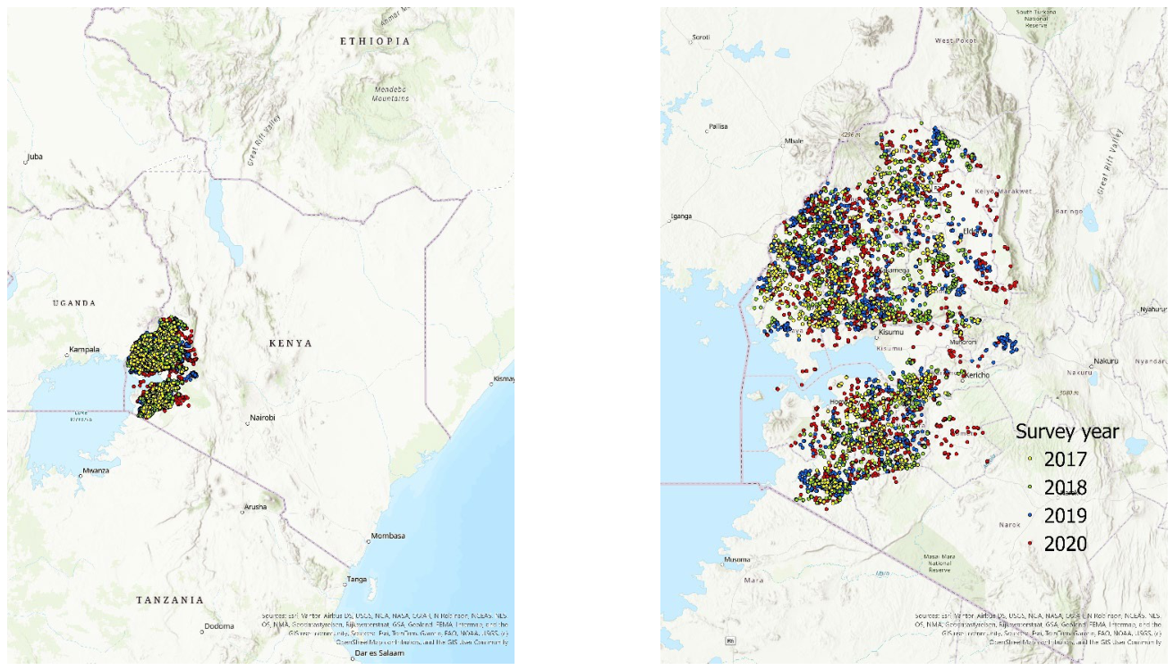
Figure 2.
Distribution of field-level maize yield by survey year. Boxplots summarize the median and interquartile range, with individual field-year observations overlaid.
Figure 2.
Distribution of field-level maize yield by survey year. Boxplots summarize the median and interquartile range, with individual field-year observations overlaid.
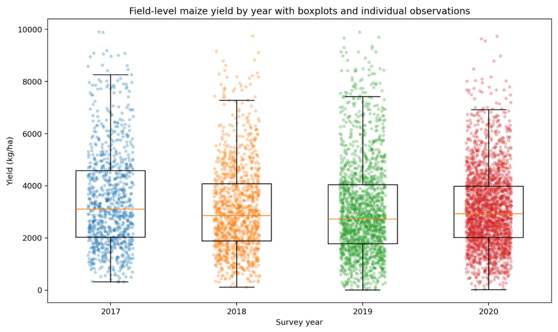
Figure 3.
Observed versus out-of-fold predicted maize yield for the XGBoost model excluding conventional remote-sensing predictors.
Figure 3.
Observed versus out-of-fold predicted maize yield for the XGBoost model excluding conventional remote-sensing predictors.
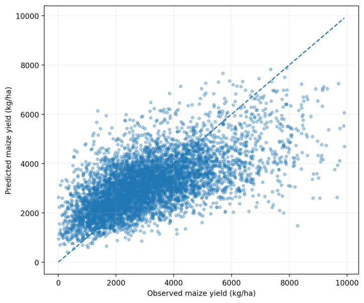
Figure 4.
Scatter plots of observed versus predicted maize yield for the best-performing XGBoost configuration, shown separately for 2017, 2018, 2019, and 2020 based on pooled out-of-fold predictions. The dashed line denotes the 1:1 line.
Figure 4.
Scatter plots of observed versus predicted maize yield for the best-performing XGBoost configuration, shown separately for 2017, 2018, 2019, and 2020 based on pooled out-of-fold predictions. The dashed line denotes the 1:1 line.
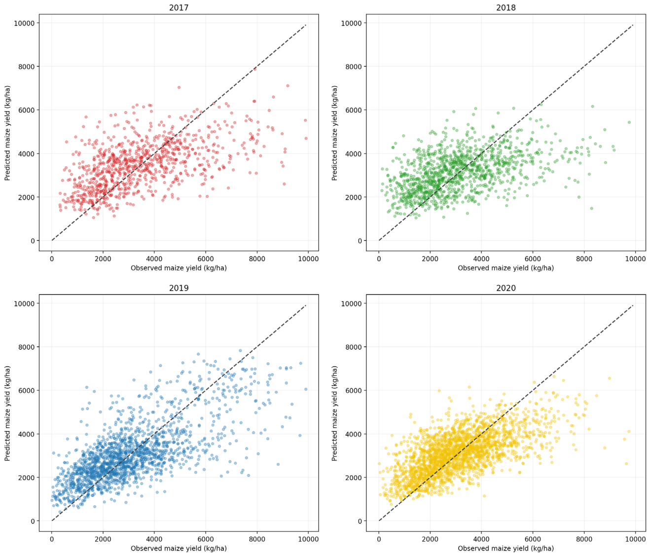
Figure 5.
SHAP dependence of nitrogen fertilization rate in the all-predictor XGBoost model. Points represent individual observations, the solid line shows the LOWESS-smoothed relationship, the shaded band represents the 95% bootstrap confidence interval, and the dashed horizontal line denotes zero SHAP contribution relative to the model baseline.
Figure 5.
SHAP dependence of nitrogen fertilization rate in the all-predictor XGBoost model. Points represent individual observations, the solid line shows the LOWESS-smoothed relationship, the shaded band represents the 95% bootstrap confidence interval, and the dashed horizontal line denotes zero SHAP contribution relative to the model baseline.
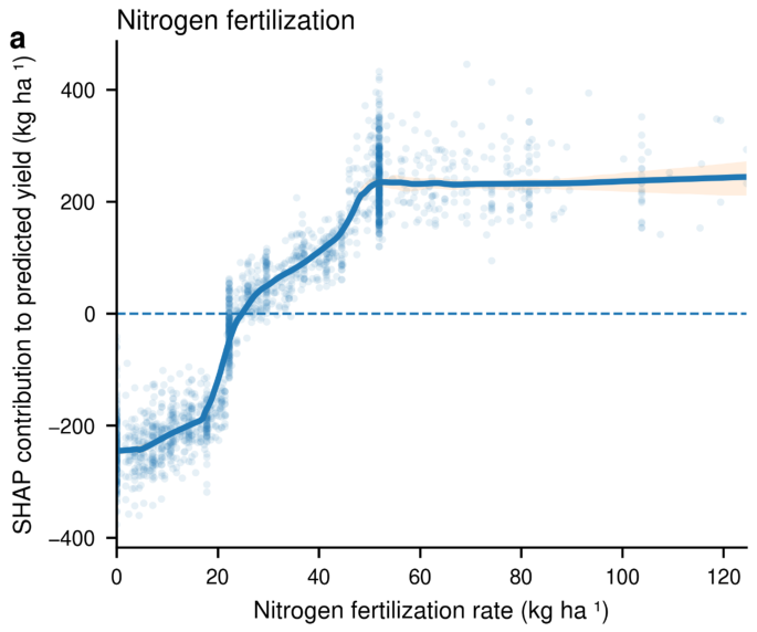

Table 1.
Predictor Groups and Numbers of Variables in the Pooled Model Matrix.
| Predictor group | Construction in the pooled model matrix | Number of predictors |
| Conventional remote sensing | 23 monthly satellite variables × 12 months | 276 |
| Climate | 25 monthly weather and hydrometeorological variables × 12 months | 300 |
| Survey-based management | Survey-based plot-level and derived management variables | 52 |
| Satellite embeddings | 64 annual embedding dimensions | 64 |
| Soil | Static soil-property variables | 14 |
| Terrain and location | Elevation, slope, travel time, topographic wetness, latitude, and longitude | 7 |
| All predictors | Full pooled model matrix | 713 |
Table 2.
Selected Percentiles of Pooled Maize-Plot Area.
| Percentile | Plot area (ha) | Percentile | Plot area (ha) |
| 5th | 0.051 | 75th | 0.405 |
| 10th | 0.101 | 90th | 0.607 |
| 25th | 0.101 | 95th | 0.809 |
| 50th | 0.202 | 99th | 1.416 |
Table 3.
Cross-Validated Performance of Eleven Candidate Algorithms for Pooled Maize-Yield Prediction.
Table 3.
Cross-Validated Performance of Eleven Candidate Algorithms for Pooled Maize-Yield Prediction.
| Model | Pooled R² | RMSE (kg ha⁻¹) | MAE (kg ha⁻¹) |
| XGBoost | 0.383 | 1,334 | 1,013 |
| Extra Trees | 0.375 | 1,342 | 1,022 |
| Random Forest | 0.323 | 1,397 | 1,082 |
| Multilayer perceptron neural network | 0.239 | 1,502 | 1,159 |
| K-nearest neighbors | 0.238 | 1,482 | 1,149 |
| Ridge regression | 0.191 | 1,542 | 1,154 |
| Linear support-vector regression | 0.181 | 1,558 | 1,178 |
| Lasso regression | 0.167 | 1,561 | 1,155 |
| Linear regression | 0.071 | 1,630 | 1,161 |
| Mean-prediction baseline | −0.003 | 1,700 | 1,333 |
| Approximate radial-basis-function support-vector regression | −0.022 | 1,742 | 1,347 |
Table 4.
Pooled Cross-Validated XGBoost Performance by Predictor Configuration.
| Predictor configuration | Number of predictors | R² | RMSE (kg ha⁻¹) | MAE (kg ha⁻¹) |
| Climate + management + satellite embeddings + soil, terrain, and location; no conventional remote sensing | 437 | 0.386 | 1,330 | 1,009 |
| Conventional remote sensing + climate + management + soil, terrain, and location; no satellite embeddings | 649 | 0.386 | 1,331 | 1,011 |
| All predictors | 713 | 0.383 | 1,334 | 1,013 |
| Conventional remote sensing + satellite embeddings + management + soil, terrain, and location; no climate | 413 | 0.360 | 1,359 | 1,037 |
| Conventional remote sensing + climate + soil, terrain, and location; no management or satellite embeddings | 597 | 0.250 | 1,470 | 1,144 |
| Conventional remote sensing + soil, terrain, and location; no climate, management, or satellite embeddings | 297 | 0.229 | 1,491 | 1,166 |
| Conventional remote sensing only | 276 | 0.196 | 1,523 | 1,192 |
Table 5.
Year-Specific Performance of the Best-Performing XGBoost Configuration From Pooled Cross-Validation.
Table 5.
Year-Specific Performance of the Best-Performing XGBoost Configuration From Pooled Cross-Validation.
| Survey year | Number of observations | R² | RMSE (kg ha⁻¹) | MAE (kg ha⁻¹) |
| 2017 | 903 | 0.300 | 1,561 | 1,191 |
| 2018 | 1,172 | 0.215 | 1,484 | 1,142 |
| 2019 | 1,681 | 0.501 | 1,299 | 987 |
| 2020 | 2,260 | 0.409 | 1,157 | 884 |
| All years | 6,016 | 0.386 | 1,330 | 1,009 |
Table 6.
Grouped SHAP Importance by Predictor Family in the All-Predictor XGBoost Model.
| Predictor family | Mean absolute SHAP (kg ha⁻¹) | Percentage importance (%) |
| Climate | 547.8 | 39.0 |
| Management | 456.1 | 32.4 |
| Remote sensing | 249.7 | 17.8 |
| Satellite embeddings | 77.4 | 5.5 |
| Soil | 58.0 | 4.1 |
| Terrain and location | 17.1 | 1.2 |
Table 7.
Leading Management Predictors in the All-Predictor XGBoost Model.
| Management predictor | Mean absolute SHAP (kg ha⁻¹) |
| Plant density | 292.4 |
| Nitrogen fertilizer (kg ha⁻¹) | 178.9 |
| Hybrid seed use | 63.9 |
| Planting date | 47.3 |
| Phosphorus fertilizer (kg ha⁻¹) | 33.2 |
| Fertilizer applied in planting hole | 27.9 |
Disclaimer/Publisher’s Note: The statements, opinions and data contained in all publications are solely those of the individual author(s) and contributor(s) and not of MDPI and/or the editor(s). MDPI and/or the editor(s) disclaim responsibility for any injury to people or property resulting from any ideas, methods, instructions or products referred to in the content. |
© 2026 by the authors. Licensee MDPI, Basel, Switzerland. This article is an open access article distributed under the terms and conditions of the Creative Commons Attribution (CC BY) license (http://creativecommons.org/licenses/by/4.0/).
Copyright: This open access article is published under a Creative Commons CC BY 4.0 license, which permit the free download, distribution, and reuse, provided that the author and preprint are cited in any reuse.