

Submitted:
31 October 2026
Posted:
02 November 2026
You are already at the latest version
Abstract
Binary-weighted measurement systems, such as successive-approximation converters built from discrete resistors, sets of reference weights or banks of binary thresholds, are usually specified with one tolerance class for all elements. Because an element's contribution to the conversion error scales with its binary weight, this over-buys precision for the less significant elements. This paper treats per-element tolerance as a cost-constrained allocation problem. For a power-law cost, in which price scales as t−α with tolerance t, the error-variance-optimal allocation is ti ∝ Wi−2/(α+2), and the cost ratio to a uniform design of equal error variance, obtained in closed form, falls approximately as 1/N with the number of bits N. Monte Carlo simulation of a 10-bit converter confirms the closed form (cost ratios of 0.379 for α = 1 and 0.299 for α = 2 at equal RMSE). Because linearity yield is not a variance criterion, tolerance classes are also selected under a yield constraint and validated on 3000 independent units: at ≥ 99 % yield (|INL|, |DNL| ≤ 0.5 LSB) the allocated designs cost 48–74 % less than the cheapest uniform design for α = 0.5 to 2, and 64–67 % less with the catalogue prices of 120 commercial resistors (fitted α ≈ 1.2). SPICE Monte Carlo of a SKY130 capacitor array shows that integrated unit-cell arrays already realise the α = 2 optimum under area-only mismatch; a layout-level study shows that coarser cells for the significant bits help at equal area only when edge mismatch is significant and gradients are moderate.
Keywords:
tolerance allocation
; binary-weighted measurement
; successive approximation
; component tolerance
; measurement yield
; cost optimization
; mismatch
1. Introduction
Many measurement systems resolve an unknown quantity by comparing it with a set of physical references whose values follow powers of two. The successive-approximation-register (SAR) analogue-to-digital converter is the best-known example [1,2], but the same structure appears in binary-weighted resistor networks, in weighing with a set of binary reference masses, and in threshold banks that convert a physical quantity into a binary code through a binary search. In each case the accuracy of the result depends on how closely the realised references follow their nominal binary ratios.
When such a system is assembled from discrete parts, each reference element is purchased or manufactured to a tolerance class, and the usual engineering practice is to specify one class for all elements. The contribution of an element to the output error, however, scales with its weight: an error of 0.1 % in the most significant element of a 10-bit system displaces the result by about half a least significant bit (LSB), whereas the same relative error in the least significant element displaces it by one thousandth of an LSB. A uniform specification therefore buys precision where it has almost no effect.
Allocating tolerances to minimise cost for a required functional accuracy is an established problem in mechanical design, where the cost of each dimension is modelled as a decreasing function of its tolerance and the assembly tolerance is a combination of the component tolerances [3,4,5,6]. The reciprocal-square cost model proposed by Spotts [3], for example, leads to allocations in which each tolerance is weighted by its sensitivity. In integrated circuits, the analogous trade-off between matching accuracy and device area follows from the Pelgrom mismatch law [7,8]. Post-fabrication calibration, which estimates and corrects the realised weights of each unit, is the other established remedy [9,10]; it acts after assembly, whereas allocation acts on the specification. Methods for discrete tolerance classes, where the cost–tolerance relation is a step function, have also been developed, for example the slope-based method of Nagarwala et al [6]. To the author's knowledge, the tolerance-allocation view has not been applied explicitly to binary-weighted measurement systems built from discrete references, in which the sensitivity of each element is fixed by its binary weight.
The hypothesis examined in this paper, proposed by the author, is that the precision of each reference element in a binary-weighted measurement system should follow its significance rather than being uniform, and that doing so reduces component cost substantially at unchanged measurement quality. The contributions are as follows.
(i) A closed-form, error-variance-optimal tolerance allocation ti ∝ Wi−2/(α+2) for a power-law cost model, together with an explicit expression for the achievable cost ratio and its asymptotic 1/N behaviour (Section 3).
(ii) A yield-constrained allocation over catalogue tolerance classes, evaluated by Monte Carlo static testing and validated on independent units, showing that the variance-optimal rule and the yield-optimal selection differ and why (Section 4 and Section 5).
(iii) A validity boundary for integrated capacitor arrays. SPICE Monte Carlo shows that unit-cell arrays already satisfy the α = 2 optimum under area-only mismatch (Section 5.5), and a layout-level study shows that coarser cells for the significant bits help at equal area only when edge mismatch is significant and gradients are moderate (Section 5.6).
2. System model
2.1. Binary-weighted conversion with toleranced references
An N-bit binary-weighted system is considered with index i = 1 for the least significant bit (LSB) and i = N for the most significant bit (MSB). The nominal weights, in units of the LSB q, are
Wi = 2i−1 q, i = 1, …, N. (1)
Each weight is realised by one physical element whose relative deviation δi is bounded by the tolerance class ti of that element:
Ŵi = Wi(1 + Δi), |Δi| ≤ ti. (2)
As a conservative model, δi is taken as uniformly distributed on [−ti, ti]; a truncated Gaussian with standard deviation ti/3 is used as a robustness case. The conversion is a binary search: starting from the MSB, the element is retained if the residue exceeds the realised weight plus comparator noise, and removed otherwise. The digital output is reconstructed with the nominal weights, as in a system whose firmware knows only the nominal part values. Comparator noise of 0.25 LSB rms and input noise of 0.01 LSB rms are included.
2.2. Error variance
For a uniformly distributed input, each decision bi equals 1 with probability 1/2, so E[bi2] = 1/2. To first order, the error caused by the reference deviations is the weighted sum of the deviations of the retained elements, and its variance is
(3)
where the second equality uses var(δi) = ti2/3 for the uniform model. The factor Wi2 expresses the unequal significance of the elements: the MSB of a 10-bit system carries 218 ≈ 2.6 × 10⁵ times the variance weight of the LSB. Equation (3) treats the decisions as independent of the deviations. This is a first-order approximation, since the decisions depend on the residue and therefore on the realised weights. The deviations considered here (at most 1 % of each weight) move each decision threshold by a small fraction of that weight, however, so the dependence enters only at second order. Section 5.1 tests the approximation directly against the full Monte Carlo model, which contains all of these effects.
2.3. Cost model
The cost of a toleranced element is modelled by the reciprocal power law
(4)
where κ is a price scale and α > 0 describes how steeply price rises as tolerance tightens. The special case α = 2 is the reciprocal-square model of mechanical tolerancing [3] and is also the matching-area model of integrated devices, since the Pelgrom law gives σ ∝ A−1/2 and hence area ∝ σ−2 [7]. To anchor α, the unit prices of 120 surface-mount resistors (case 0805, 10 kΩ) in the seven tolerance classes of Section 4 were taken from a distributor catalogue [11] (Table 4). A least-squares fit of log price against log(1/t) gives α = 1.16 for the class median (R2 = 0.95, bootstrap 95 % interval 0.88–1.34) and α = 1.30 for the cheapest part in each class (R2 = 0.91, 1.02–1.50). The case α = 1 is therefore representative of discrete resistors. Because prices within one class vary by more than an order of magnitude between series, results are reported for 0.5 ≤ α ≤ 3, and Section 5.2 also repeats the selection with the catalogue prices themselves.
3. Closed-Form Allocation
3.1. Optimal Tolerances
Minimising the cost (4) subject to a prescribed error variance (3) is a convex problem in the variables ti > 0. With the Lagrangian L = κΣti−α + μ(ΣWi2ti2 − 6σ2), the stationarity condition −ακti−α−1 + 2μWi2ti = 0 gives tiα+2 ∝ Wi−2, that is
(5)
with λ fixed by the variance constraint. For binary weights, the optimal tolerance tightens by the constant factor 22/(α+2) from one bit to the next: a factor of 1.59 for α = 1 and √2 for α = 2. The rule has a direct interpretation. At the optimum the marginal cost of reducing the variance is the same for every element, so no reallocation of spending between elements can reduce the cost further.
3.2. Achievable Cost Ratio
A uniform design with the same variance uses tu2 = 6σ2/ΣWi2. Substituting (5) and the uniform design into (4) gives the ratio of the optimal to the uniform cost at equal error variance,
(6)
For α = 2, (6) reduces to R = (ΣWi)2/(NΣWi2), which is at most 1 by the Cauchy–Schwarz inequality, with equality only if all weights are equal. For binary weights and large N, ΣWi ≈ 2N and ΣWi2 ≈ 4N/3, so R ≈ 3/N. More generally, R(α, N) ≈ 3α/2/[N(2p − 1)1+α/2]: the saving of the significance-weighted design grows with resolution. Figure 1 shows the saving 1 − R for 6 ≤ N ≤ 16. For N = 10 the saving is 49.5 %, 62.1 % and 70.1 % for α = 0.5, 1 and 2.
4. Simulation Methodology
All results in Section 5.1 to 5.4 were obtained with a behavioural Monte Carlo model of the converter of Section 2. Each simulated unit draws one set of deviations δi, which is fixed for that unit. Two figures of merit are computed per unit.
(a) Static linearity. Differential and integral nonlinearity (DNL, INL) are obtained by a code-density test with 32 samples per code. Comparator and input noise are switched off in this test, so the yield reflects the reference deviations alone, and INL is referred to the endpoint line [12]. A unit passes if both |INL| and |DNL| are at most 0.5 LSB. The yield is the fraction of passing units; its 95 % confidence interval is given by the Wilson score interval.
(b) Conversion RMSE. The root-mean-square difference between the reconstructed output and the input is computed over 4000 uniformly distributed inputs with comparator and input noise included. With ideal references the RMSE is 0.382 LSB, set by quantisation (1/√12 = 0.289 LSB) and comparator noise (0.25 LSB) added in quadrature. Differences in RMSE between designs are therefore differences in the reference contribution above this floor.
The available tolerance classes are 1 %, 0.5 %, 0.25 %, 0.1 %, 0.05 %, 0.02 % and 0.01 %. For the yield-constrained designs, classes are selected by a greedy procedure. Starting from 1 % for every element, it repeatedly tightens the one element that gives the largest yield increase per unit of added cost. It stops when the yield on a training set of 500 units reaches 99.5 %. The selection is constrained so that a more significant element is never assigned a looser class than a less significant one. Every selected design, and every uniform reference design, is then re-evaluated on an independent validation set of 3000 units generated with a different random seed. All reported yields, RMSE values and costs come from that validation set. The margin between the 99.5 % training target and the 99 % acceptance level absorbs the sampling error of the training set.
The simulation code (Python, ngspice and MATLAB) was written with the assistance of a generative AI tool (Claude, Anthropic), as stated in the Acknowledgements. The author defined the models and acceptance criteria and checked the code and its outputs; the code is openly available (see the Data availability statement).
5. Results
5.1. Verification of the closed form
The continuous allocation (5) was evaluated for N = 10 against a uniform tolerance of 0.1 %, scaled so that both designs have the same error variance (3). The results over 2000 units are given in Table 1. The RMSE of the two designs agrees to within 0.5 % (0.452 and 0.450 LSB for α = 1), and the Monte Carlo cost ratios, 0.379 for α = 1 and 0.299 for α = 2, coincide with (6). The closed form is therefore confirmed for the quantity it optimises, including the first-order independence assumption behind (3). The uniform 0.1 % yield here (85.4 %, 2000 units) differs slightly from that in Table 2 (87.1 %, 3000 units) because the two are independent random samples; their 95 % confidence intervals overlap.
The same table shows that the variance-optimal design has a lower linearity yield than the uniform design (77.5 % against 85.4 % for α = 1). The reason is the endpoint reference line used for INL. It removes the gain error of each unit, and for a uniform relative tolerance the gain error is dominated by the MSB, the same element that dominates the nonlinearity. Much of the MSB's deviation therefore disappears into the gain correction. When the LSB-side elements are loosened, their deviations are no longer proportional to those of the MSB and are not removed by the gain correction. Variance-optimal and yield-optimal allocations therefore differ. A variance criterion suits applications that report absolute error without gain calibration, whereas a linearity-yield criterion suits systems in which a one-point gain calibration is routine. The latter is treated next.
5.2. Yield-Constrained Selection from Tolerance Classes
Table 2 lists the uniform reference designs for N = 10. A single class of 0.1 % yields only 87.1 % of units within ±0.5 LSB, so a uniform design requires 0.05 % throughout to exceed 99 % yield. Table 3 gives the designs selected for α = 0.5, 1 and 2 and their validation results.
At α = 1 the selected design keeps the three least significant elements at 1 %, and only the two most significant elements need the 0.05 % class used everywhere in the uniform design. The validated yield is 99.8 % (95 % CI 99.5–99.9 %) and the RMSE is 0.405 LSB, against 0.400 LSB for the uniform 0.05 % design. The saving is 63.5 %. The savings for α = 0.5 and 2 are 48.0 % and 73.8 %. They are smaller than the variance-optimal values of Figure 1 because the classes are discrete and because of the yield criterion discussed in Section 5.1. They are nevertheless large for every cost exponent considered. To measure how far the greedy selection is from the true optimum, all 8008 ordered class vectors for N = 10 were searched exhaustively in order of increasing cost under the same training criterion. For α = 0.5 and α = 1 the greedy designs are the exact optima. For α = 2 the optimum loosens the three least significant elements from 0.5 % to 1 % and costs 1039 instead of 1048 units (0.9 % less), which raises the saving from 73.8 % to 74.0 %. The greedy procedure is therefore at or within 1 % of the optimum. Figure 2 compares the selected classes with the continuous rule (5), and Figure 3 places the selected design on the yield–cost plane of the uniform designs. Finally, the exhaustive search was repeated with the catalogue prices of Table 4 in place of the power law. Market prices are step-like and not even monotonic (the cheapest 0.01 % part costs less than the cheapest 0.02 % part), so this is a direct test of the conclusions against real costs. With median prices the optimum is the design of Table 3 for α = 1, at 310.7 INR against 853.7 INR for uniform 0.05 %, a saving of 63.6 %. With the cheapest part in each class the optimum (1 / 1 / 1 / 0.5 / 0.5 / 0.1 / 0.1 / 0.1 / 0.05 / 0.05 %) saves 66.6 % (102.3 against 306.7 INR). Validated yields are 99.8 % and 99.8 %.
5.3. Robustness to the Tolerance Distribution
Manufactured parts are often distributed more narrowly than their tolerance bound. The design selected for α = 1 under the uniform model was therefore re-validated with deviations drawn from a truncated Gaussian of standard deviation ti/3, without re-selection. The yield was 100.0 % (95 % CI 99.9–100.0 %). Under the same model the uniform 0.1 % design reaches 98.9 % and still falls short of 99 %, so the cheapest passing uniform design remains 0.05 % and the saving is unchanged at 63.5 %. Selection under the uniform model is thus conservative with respect to more concentrated distributions.
5.4. Resolution
Table 5 repeats the selection for other resolutions at α = 1. In agreement with the 1/N trend of Section 3.2, the saving grows with resolution, from 40.6 % at 8 bits to 63.5 % at 10 bits and 76.5 % at 12 bits, because the spread of significance between the most and least significant elements grows as 2N−1. At 12 bits the uniform design needs the tightest class considered (0.01 %) for every element, and the uniform 0.02 % design reaches only 95.7 % yield. The allocated design uses that class only for the MSB and keeps the four least significant elements at 0.5 %. At higher resolution the tightest available class, rather than cost, becomes the limit for a uniform design, whereas an allocated design needs it for only one or two elements.
5.5. Validity Boundary: Integrated Unit-Cell Arrays
The rule assumes that each element can be assigned its own tolerance independently of its nominal value. This holds for discrete parts but not for an integrated capacitor array built from unit cells. To test the boundary, a 10-bit charge-redistribution array was simulated in ngspice [13] using the metal–insulator–metal capacitor model of the open SkyWater SKY130 process design kit [14]. That model specifies a mismatch of σC/C = 2.8 %/√(WL/µm2). Each bit was built from 2i−1 unit cells of 4 µm × 4 µm, and 300 Monte Carlo instances were run. The relative standard deviation of each bit capacitance follows the Pelgrom scaling, from 0.73 % for the LSB to 0.0314 % for the MSB, against 0.0321 % predicted from the LSB value by W−1/2 (Figure 4).
This scaling is exactly the optimum (5) for α = 2, which is the matching-area cost of integrated devices. A unit-cell array therefore already realises the significance-weighted allocation, with no design effort. Uniform enlargement of the whole array by a factor of 8 in area changed the conversion RMSE by less than 3 % (0.393 and 0.383 LSB), confirming that mismatch was not limiting. Conversely, enlarging only the cells of the three MSBs (3 × 3 area) destroys the binary ratios themselves, because in a capacitor array the weight is the capacitance: DNL rose to about 126 LSB and the SNDR fell from 59.2 dB to 19.8 dB. Nonuniform precision in an integrated array can only be obtained by means that keep the capacitance ratios, such as building each bit from cells of a different size, which introduces systematic ratio errors of its own. Under area-only mismatch the allocation rule therefore gives no gain for integrated unit-cell arrays; Section 5.6 examines when this changes. For systems whose elements are specified individually, the uniform-class practice is far from optimal.
5.6. Integrated Capacitor Arrays: Edge Mismatch, Gradients and the Limit of the Rule
Area-only mismatch. In an integrated capacitive DAC the cost of precision is area. If the relative mismatch of a capacitor of area Ai follows the area law σ2(ΔCi/Ci) = K2/Ai [7], the error variance Σ Ci2K2/Ai is minimised under a fixed total area Σ Ai = Atot by
Ai ∝ Ci, (7)
which follows from the Cauchy–Schwarz inequality and is exactly the conventional array of identical unit cells. Under this model no reallocation of area between bits can improve accuracy at equal area; this is the α = 2 case of the allocation rule, in agreement with Section 5.5. The mismatch model of the SKY130 metal–insulator–metal capacitor is of this form, σ(ΔC)/C = 2.8 %/√(WL) with W and L in µm [14], and measurements on small metal fringe capacitors are also consistent with area scaling [15].
Edge mismatch. The conclusion rests on the area law alone. Random edge roughness adds a variance proportional to the perimeter [16]. For a square cell of s unit capacitances,
(8)
where σu is the relative standard deviation of one unit cell and ρ is the share of its variance that comes from the edge. A bit of weight Wi built from Wi/si cells of size si then has
(9)
so building a bit from fewer, larger cells reduces its edge contribution at unchanged capacitance. Three effects oppose this: a larger cell has a smaller fringe share and needs slightly more area for the same capacitance; cells of different size carry a systematic ratio error when the fringe coefficient deviates from its nominal value; and fewer, larger cells are harder to place in a common centroid, which exposes them to process gradients. The design family studied here uses cells of size si = min(Wi, S), so the significant bits are built from cells of S units and the bits smaller than S are single cells; S = 1 is the conventional array.
Method. A 10-bit array of 210 unit sites was simulated in MATLAB with σu = 0.8 %, which gives the conventional array a linearity yield of about 94 %. The systematic fringe error of a cell of size s was fηz(s−1/2 − 1), with fringe fraction f = 0.05, uncertainty η of the fringe coefficient and z ~ N(0, 1) per die. The area overhead of larger cells was computed from the same fringe model (at most 4.9 % for S = 512), and each design was then shrunk to the area of the conventional array, which multiplies the area term of (8) by the area ratio r and the edge term by r3/2. For every S an explicit layout was generated: bits with at least two cells receive point-symmetric pairs of cells from the centre outwards, so that a linear gradient cancels exactly, and the bits smaller than S share one central block split in binary halves. The capacitance density was 1 + gxu + gyv + qxxu2 + qyyv2 + qxyuv over the normalised array coordinates u and v, with gx, gy ~ N(0, gs) and qxx, qyy, qxy ~ N(0, gs/2) per die, where gs is the relative density change at the array edge. Yield was defined as max|DNL| ≤ 0.5 LSB and max|INL| ≤ 0.5 LSB (endpoint fit, all codes). For each parameter set the best S was selected on 10 000 training dies and compared with the conventional array on 40 000 independent test dies drawn with the same random numbers for both designs (paired comparison, 95 % Wilson intervals).
Results. Table 6 isolates the edge effect without gradients (η = 0.10). With ρ = 0 the procedure selects the conventional array, as (7) requires. With ρ > 0 the coarse-cell designs are better at equal area, and the gain grows with ρ.
Table 7 adds gradients and common-centroid placement. Gradients penalise large cells and move the optimum towards smaller S; whenever a gradient was present and a gain remained, the selected cell size was S = 8. For ρ = 0.25 the rms INL falls by 8.2 %, 6.3 % and 2.9 % for gs = 0, 0.001 and 0.003; for ρ = 0.5 it falls by 21.2 %, 15.5 % and 11.7 %. For ρ = 0.10 the gain is at most 0.4 percentage points of yield, and for gs = 0.01 the conventional array is selected at every ρ. In no case did the selected design perform worse than the conventional array on the test set.
Scope. These results define where a nonuniform allocation can improve an integrated array at equal area; they do not show that a particular process lies in that region. No published, verifiable fit of the edge share ρ or of the gradient magnitude gs was found for the capacitor types used in SAR DACs, and the SKY130 model [14] corresponds to ρ = 0, for which no gain exists. For integrated arrays the rule is therefore conditional: it applies to processes or capacitor structures with a significant edge component and moderate gradients, and ρ must be determined for each process. A simple test structure suffices: single cells of 1, 4, 16 and 64 unit capacitances, whose measured variances, plotted against (8), separate the area and edge terms. Routing and top-plate parasitics, the dependence of the fringe fraction on cell size after shrinking, and comparator noise were not modelled. For arrays assembled from individually specified discrete parts none of these restrictions applies, which is why the main results of this paper concern such systems.
6. Discussion
Scope of application. The results apply to any binary-weighted measurement system whose references are individually specified parts: resistor-array converters and sensor interfaces, sets of binary reference masses, banks of binary optical or radiation attenuators, and hydraulic or mechanical threshold banks resolved by binary search. In all of these, the designer chooses one tolerance per element and pays per element. Equation (5) then gives the direction and the rate of tightening, and the yield-constrained selection gives a purchasable design.
Practical significance. For low-cost chip resistors the absolute saving per unit is small. For the 12-bit design with the catalogue prices of Table 4, the resistor set costs 406 INR instead of 1145 INR with the cheapest parts, and 1722 INR instead of 5515 INR with median parts (about US$4.2 against US$11.9, and US$18 against US$57, at 95.95 INR per US$ on 30 September 2026). This figure uses the 12-bit selection of Table 5 with one market correction: because 0.02 % parts cost more than 0.01 % parts in Table 4, the two 0.02 % elements are replaced by 0.01 % parts, which is both cheaper and tighter. The corrected design was re-validated on 3000 units, with a yield of 100.0 % (95 % CI 99.9–100.0 %). The saving matters in three situations. First, in series production it scales with volume and requires only a different bill of materials, with no change to the circuit or the firmware. Second, where each reference element is itself expensive, such as bulk-metal-foil resistors, calibrated reference weights of a high accuracy class, or radiation and optical attenuators, the same percentage corresponds to a large absolute amount. Third, and most important at high resolution, the constraint becomes availability rather than price. At 12 bits a uniform design already needs the tightest catalogue class for every element, whereas the allocated design needs it for three. Beyond this resolution a uniform design would need a class tighter than any in Table 4, while an allocated design can still be built from available parts for its less significant elements.
Choice of criterion. Section 5.1 shows that the allocation depends on how quality is judged. If absolute error without gain calibration matters, the variance rule (5) is optimal. If linearity after a gain correction is the acceptance criterion, as is common in instrumentation, the selection should be made on yield. In both cases the least significant elements can be relaxed by one or more tolerance classes. A practical procedure is to compute (5) for the parts considered, round each tolerance to the nearest catalogue class, and then check or refine the design by yield simulation as in Section 5.2.
Relation to calibration. Allocation acts on the distribution of the deviations before assembly, whereas calibration measures and corrects the deviations of a finished unit. A system whose MSB elements are tight needs a smaller correction range, and one whose LSB elements are loose adds deviations of below 0.1 LSB. The two measures are therefore complementary.
Limitations. (1) The power law fits catalogue prices only approximately, and prices depend on series and supplier; the direct search with catalogue prices (Section 5.2) gives savings consistent with the fitted α, but a designer should repeat it with the parts actually considered. (2) Temperature coefficient and long-term drift, which also scale with tolerance class in practice, are not modelled. (3) Nominal-value quantisation of standard resistor series is assumed to be known to the firmware and is not treated as error. (4) The greedy selection is not guaranteed to be optimal in general; for N = 10 it was checked against exhaustive search (Section 5.2). (5) The simulations are behavioural. Experimental confirmation with purchased parts is the natural next step.
7. Conclusion
The author's hypothesis that reference precision in a binary-weighted measurement system should follow significance was formulated as a tolerance-allocation problem and confirmed. For a power-law cost, the variance-optimal tolerances follow ti ∝ Wi−2/(α+2), with a closed-form cost ratio that falls as about 1/N. Under a linearity-yield criterion with catalogue classes and independent validation, a 10-bit design at ≥99 % yield costs 48.0–73.8 % less than the cheapest uniform design, and the saving increases with resolution. The same analysis shows that integrated unit-cell arrays already sit at the α = 2 optimum under area-only mismatch; there, coarser cells for the significant bits give a gain at equal area only when edge mismatch is significant and gradients are moderate. The rule applies directly to systems built from individually specified references, which are common in measurement practice.
Funding
This research received no external funding.
Data Availability Statement
The simulation code (Python, ngspice netlist generator and MATLAB) and the catalogue price data used in this work are openly available in Zenodo at https://doi.org/10.5281/zenodo.23831765.
Acknowledgments
During the preparation of this manuscript, the author used Claude (Anthropic, Claude Opus 5.5) to support writing the simulation code (behavioural Monte Carlo in Python and MATLAB, and SPICE Monte Carlo in ngspice), running the Python and SPICE simulations, preparing the figures, and drafting the manuscript text. The MATLAB simulations of Section 5.6 were run by the author. The research hypothesis, the problem formulation and the choice of application were the author's. The author reviewed, validated and critically assessed all AI-assisted outputs, including the derivations, the numerical results and the references.
Conflicts of Interest
The author declares no conflicts of interest.
References
- Razavi, B. Principles of Data Conversion System Design; IEEE Press: New York, 1995. [Google Scholar]
- McCreary, J. L.; Gray, P. R. All-MOS charge redistribution analog-to-digital conversion techniques—Part I. IEEE J. Solid-State Circuits 1975, 10, 371–9. [Google Scholar] [CrossRef]
- Spotts, M. F. Allocation of tolerances to minimize cost of assembly. J. Eng. Ind. 1973, 95, 762–4. [Google Scholar] [CrossRef]
- Chase, K. W.; Parkinson, A. R. A survey of research in the application of tolerance analysis to the design of mechanical assemblies. Res. Eng. Des. 1991, 3, 23–37. [Google Scholar] [CrossRef]
- Chase, K. W.; Greenwood, W. H.; Loosli, B. G.; Hauglund, L. F. Least cost tolerance allocation for mechanical assemblies with automated process selection. Manuf. Rev. 1990, 3, 49–59. [Google Scholar]
- Nagarwala, M. Y.; Pulat, P. S.; Raman, S. A slope-based method for least cost tolerance allocation. Concurr. Eng. 1995, 3, 319–28. [Google Scholar] [CrossRef]
- Pelgrom, M. J. M.; Duinmaijer, A. C. J.; Welbers, A. P. G. Matching properties of MOS transistors. IEEE J. Solid-State Circuits 1989, 24, 1433–9. [Google Scholar] [CrossRef]
- Kinget, P. R. Device mismatch and tradeoffs in the design of analog circuits. IEEE J. Solid-State Circuits 2005, 40, 1212–24. [Google Scholar] [CrossRef]
- Liu, W.; Huang, P.; Chiu, Y. A 12-bit, 45-MS/s, 3-mW redundant successive-approximation-register analog-to-digital converter with digital calibration. IEEE J. Solid-State Circuits 2011, 46, 2661–72. [Google Scholar] [CrossRef]
- McNeill, J. A.; Chan, K. Y.; Coln, M. C. W.; David, C. L.; Brenneman, C. All-digital background calibration of a successive approximation ADC using the ‘split ADC’ architecture. IEEE Trans. Circuits Syst. I 2011, 58, 2355–65. [Google Scholar] [CrossRef]
- Mouser Electronics 2026 Online catalogue: SMD chip resistors, case 0805, 10 kΩ, by tolerance. Available online: https://www.mouser.in (accessed on 30 September 2026).
- IEEE 2011 IEEE Standard for Terminology and Test Methods for Analog-to-Digital Converters IEEE Std 1241-2010. [CrossRef]
- Vogt, H.; Atkinson, G.; Nenzi, P. Ngspice Users Manual Version 47 . Available online: https://ngspice.sourceforge.io.
- SkyWater Technology Foundry and Google 2020 SkyWater Open Source PDK: sky130_fd_pr primitive models. Available online: https://github.com/google/skywater-pdk-libs-sky130_fd_pr.
- Tripathi, V.; Murmann, B. Mismatch characterization of small metal fringe capacitors. IEEE Trans. Circuits Syst. I 2014, 61, 2236–42. [Google Scholar] [CrossRef]
- Shyu, J.-B.; Temes, G. C.; Krummenacher, F. Random error effects in matched MOS capacitors and current sources. IEEE J. Solid-State Circuits 1984, 19, 948–56. [Google Scholar] [CrossRef]
Figure 1.
Cost saving of the error-variance-optimal allocation (5) relative to a uniform tolerance of equal error variance, from the closed form (6), as a function of the cost exponent α for several resolutions N.
Figure 1.
Cost saving of the error-variance-optimal allocation (5) relative to a uniform tolerance of equal error variance, from the closed form (6), as a function of the cost exponent α for several resolutions N.
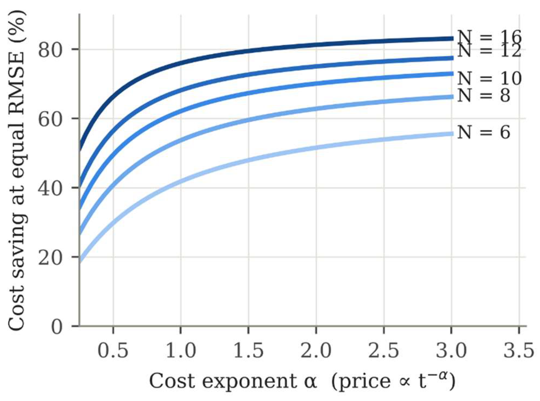
Figure 2.
Tolerance per bit: continuous variance-optimal rule (5) for α = 1 and α = 2 (at the error variance of a uniform 0.1 % design), the classes selected under the yield constraint for α = 1, and the uniform 0.05 % design needed for ≥99 % yield.
Figure 2.
Tolerance per bit: continuous variance-optimal rule (5) for α = 1 and α = 2 (at the error variance of a uniform 0.1 % design), the classes selected under the yield constraint for α = 1, and the uniform 0.05 % design needed for ≥99 % yield.
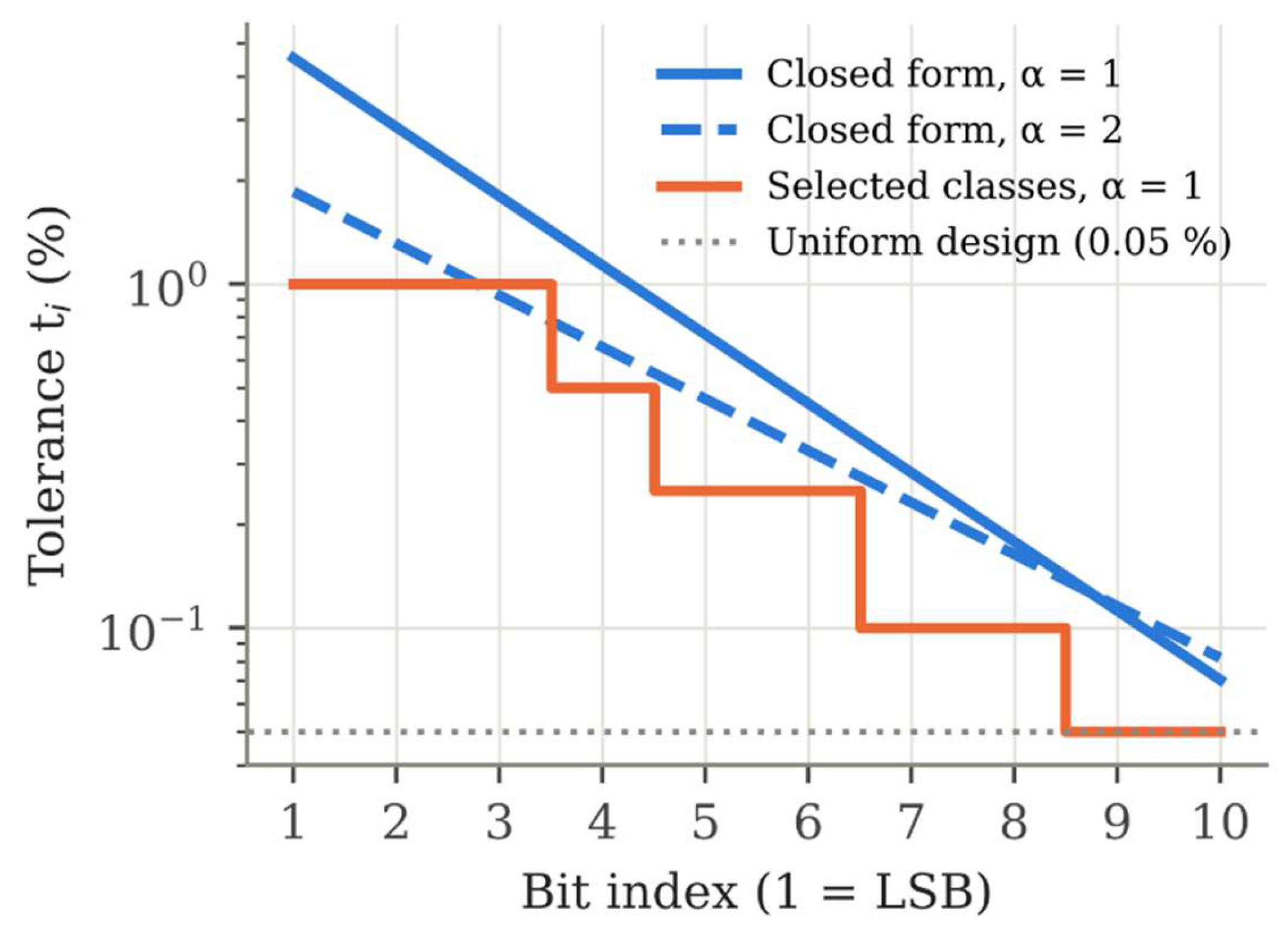
Figure 3.
Yield (|INL|, |DNL| ≤ 0.5 LSB) against relative component cost for α = 1: uniform tolerance classes and the allocated design of Table 3. Error bars are 95 % Wilson intervals on 3000 validation units; the dotted line marks 99 % yield.
Figure 3.
Yield (|INL|, |DNL| ≤ 0.5 LSB) against relative component cost for α = 1: uniform tolerance classes and the allocated design of Table 3. Error bars are 95 % Wilson intervals on 3000 validation units; the dotted line marks 99 % yield.
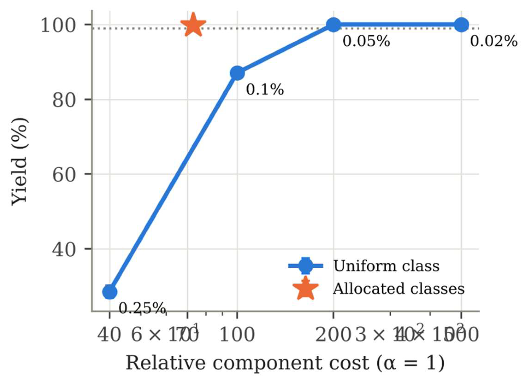
Figure 4.
Relative standard deviation of each bit capacitance of a 10-bit unit-cell MIM array (SKY130, 4 µm × 4 µm unit, 300 SPICE Monte Carlo runs) and the α = 2 optimum ti ∝ Wi−1/2 anchored at the LSB.
Figure 4.
Relative standard deviation of each bit capacitance of a 10-bit unit-cell MIM array (SKY130, 4 µm × 4 µm unit, 300 SPICE Monte Carlo runs) and the α = 2 optimum ti ∝ Wi−1/2 anchored at the LSB.
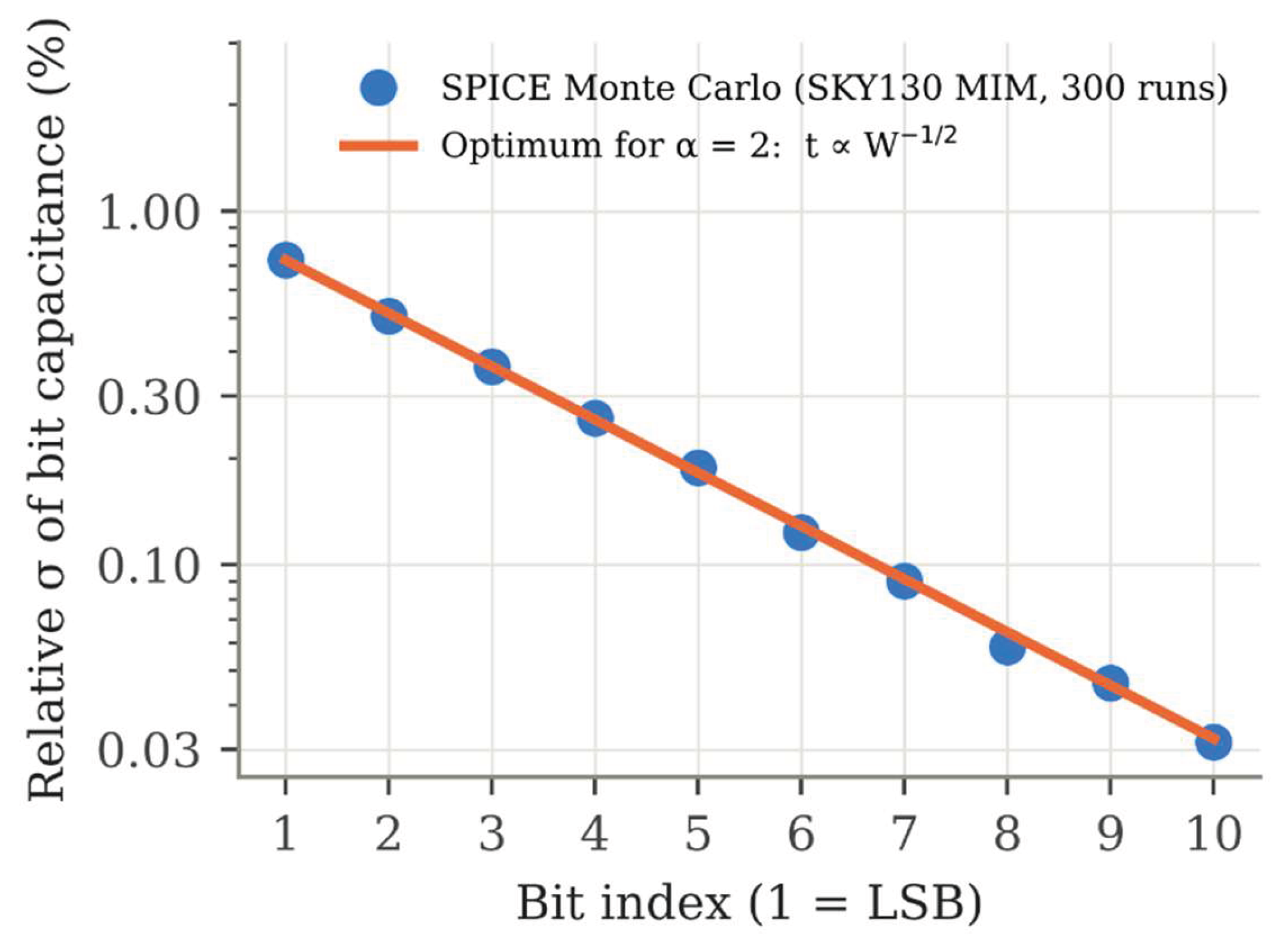

Table 4.
Catalogue unit prices of 0805, 10 kΩ surface-mount resistors by tolerance class (quantity 100, Mouser India, accessed 30 September 2026 [11]).
Table 4.
Catalogue unit prices of 0805, 10 kΩ surface-mount resistors by tolerance class (quantity 100, Mouser India, accessed 30 September 2026 [11]).
| Tolerance class | Parts | Cheapest (INR) | Median (INR) |
| 1% | 25 | 0.19 | 4.01 |
| 0.5% | 25 | 2.01 | 6.59 |
| 0.25% | 17 | 7.93 | 21.31 |
| 0.1% | 25 | 12.13 | 39.36 |
| 0.05% | 14 | 30.67 | 85.37 |
| 0.02% | 3 | 144.27 | 797.76 |
| 0.01% | 11 | 95.44 | 459.55 |
Table 1.
Continuous allocation (5) against a uniform design of equal error variance (N = 10, 2000 units).
Table 1.
Continuous allocation (5) against a uniform design of equal error variance (N = 10, 2000 units).
| Design | RMSE (LSB) | Yield (%) | Cost ratio (MC) | Cost ratio, eq. (6) |
| Uniform 0.1 % | 0.452 | 85.4 | 1 | 1 |
| Optimal (5), α = 1 | 0.450 | 77.5 | 0.379 | 0.379 |
| Optimal (5), α = 2 | 0.451 | 83.2 | 0.299 | 0.299 |
Table 2.
Uniform tolerance designs (N = 10, independent validation set of 3000 units).
| Uniform class | Yield (%) | 95 % CI (%) | INL p99 (LSB) | DNL p99 (LSB) | RMSE (LSB) |
| 0.25% | 28.6 | 27.0–30.2 | 1.05 | 1.72 | 0.682 |
| 0.1% | 87.1 | 85.8–88.2 | 0.40 | 0.75 | 0.448 |
| 0.05% | 100.0 | 99.9–100.0 | 0.20 | 0.38 | 0.400 |
| 0.02% | 100.0 | 99.9–100.0 | 0.09 | 0.16 | 0.385 |
Table 3.
Yield-constrained class selection (N = 10). Costs are in units of κ(0.01)−α per element, so that a 1 % element costs 1; validation on 3000 independent units.
Table 3.
Yield-constrained class selection (N = 10). Costs are in units of κ(0.01)−α per element, so that a 1 % element costs 1; validation on 3000 independent units.
| α | Selected classes, bit 1 → bit 10 (%) | Yield (%) [95 % CI] | RMSE (LSB) | Cost / uniform 0.05 % | Saving (%) |
| 0.5 | 1 / 1 / 1 / 0.5 / 0.5 / 0.25 / 0.25 / 0.05 / 0.05 / 0.05 | 99.2 [98.8–99.5] | 0.407 | 23.2 / 44.7 | 48.0 |
| 1.0 | 1 / 1 / 1 / 0.5 / 0.25 / 0.25 / 0.1 / 0.1 / 0.05 / 0.05 | 99.8 [99.5–99.9] | 0.405 | 73.0 / 200.0 | 63.5 |
| 2.0 | 0.5 / 0.5 / 0.5 / 0.5 / 0.25 / 0.25 / 0.1 / 0.1 / 0.05 / 0.05 | 99.8 [99.5–99.9] | 0.405 | 1048.0 / 4000.0 | 73.8 |
Table 5.
Effect of resolution on the yield-constrained selection (α = 1; 3000 validation units).
| N | Selected classes, bit 1 → bit N (%) | Yield (%) [95 % CI] | Cheapest uniform class | Saving (%) |
| 8 | 1 / 1 / 1 / 0.5 / 0.5 / 0.25 / 0.25 / 0.25 | 99.3 [98.9–99.5] | 0.25 % | 40.6 |
| 10 | 1 / 1 / 1 / 0.5 / 0.25 / 0.25 / 0.1 / 0.1 / 0.05 / 0.05 | 99.8 [99.5–99.9] | 0.05 % | 63.5 |
| 12 | 0.5 / 0.5 / 0.5 / 0.5 / 0.25 / 0.1 / 0.05 / 0.05 / 0.05 / 0.02 / 0.02 / 0.01 | 99.6 [99.3–99.8] | 0.01 % | 76.5 |
Table 6.
Equal-area comparison without gradients (η = 0.10; test set of 40 000 dies).
| ρ | Best S | r | Yield, unit array | Yield, best design | Difference (95 % CI) | rms INL (LSB), unit / best |
| 0.00 | 1 | 1.000 | 0.9442 | 0.9442 | 0 | 0.1045 / 0.1045 |
| 0.25 | 32 | 1.043 | 0.9442 | 0.9638 | +0.0196 (+0.0182, +0.0210) | 0.1045 / 0.0959 |
| 0.50 | 32 | 1.043 | 0.9442 | 0.9855 | +0.0413 (+0.0393, +0.0432) | 0.1045 / 0.0831 |
| 0.75 | 64 | 1.045 | 0.9442 | 0.9980 | +0.0539 (+0.0517, +0.0561) | 0.1045 / 0.0659 |
Table 7.
Equal-area comparison with gradients and common-centroid placement (η = 0.10; test set of 40 000 dies).
Table 7.
Equal-area comparison with gradients and common-centroid placement (η = 0.10; test set of 40 000 dies).
| ρ | gs | Best S | Yield, unit array | Yield, best design | Difference (95 % CI) | rms INL (LSB), unit / best |
| 0.10 | 0 | 8 | 0.9436 | 0.9472 | +0.0037 (+0.0030, +0.0043) | 0.1046 / 0.1030 |
| 0.10 | 0.001 | 8 | 0.9426 | 0.9460 | +0.0034 (+0.0024, +0.0043) | 0.1047 / 0.1035 |
| 0.10 | 0.003 | 1 | 0.9392 | 0.9392 | 0 | 0.1054 / 0.1054 |
| 0.10 | 0.010 | 1 | 0.9048 | 0.9048 | 0 | 0.1129 / 0.1129 |
| 0.25 | 0 | 32 | 0.9436 | 0.9633 | +0.0197 (+0.0183, +0.0211) | 0.1046 / 0.0960 |
| 0.25 | 0.001 | 8 | 0.9426 | 0.9586 | +0.0159 (+0.0147, +0.0172) | 0.1047 / 0.0981 |
| 0.25 | 0.003 | 8 | 0.9392 | 0.9491 | +0.0099 (+0.0083, +0.0115) | 0.1054 / 0.1023 |
| 0.25 | 0.010 | 1 | 0.9048 | 0.9048 | 0 | 0.1129 / 0.1129 |
| 0.50 | 0 | 64 | 0.9436 | 0.9856 | +0.0420 (+0.0400, +0.0439) | 0.1046 / 0.0824 |
| 0.50 | 0.001 | 8 | 0.9426 | 0.9772 | +0.0345 (+0.0327, +0.0363) | 0.1047 / 0.0885 |
| 0.50 | 0.003 | 8 | 0.9392 | 0.9702 | +0.0310 (+0.0291, +0.0328) | 0.1054 / 0.0931 |
| 0.50 | 0.010 | 1 | 0.9048 | 0.9048 | 0 | 0.1129 / 0.1129 |
Disclaimer/Publisher’s Note: The statements, opinions and data contained in all publications are solely those of the individual author(s) and contributor(s) and not of MDPI and/or the editor(s). MDPI and/or the editor(s) disclaim responsibility for any injury to people or property resulting from any ideas, methods, instructions or products referred to in the content. |
© 2026 by the authors. Licensee MDPI, Basel, Switzerland. This article is an open access article distributed under the terms and conditions of the Creative Commons Attribution (CC BY) license (http://creativecommons.org/licenses/by/4.0/).
Copyright: This open access article is published under a Creative Commons CC BY 4.0 license, which permit the free download, distribution, and reuse, provided that the author and preprint are cited in any reuse.