

Submitted:
13 November 2026
Posted:
17 November 2026
You are already at the latest version
Abstract
We propose a low-cost, falsifiable single-slit test of whether the photon carries a transverse circulation, as the spiral-structure model asserts. Its unit-coupling closure predicts a helicity-odd rigid translation, Δx/x₁ = λ/(2πa) — 0.80 mm at 633 nm with a 2 μm slit and a 50 mm lens, far above scientific-camera resolution. Maxwell controls return the symmetry-required null; exclusion analysis shows that no mundane medium-flow mechanism can mimic the signal at realistic screen thicknesses, and a registered thickness series discriminates mechanism classes. The estimation chain is validated on photon-counting simulations. The hardware sits at the advanced-undergraduate level; either outcome is informative.
Keywords:
photon circulation
; helicity
; single-slit diffraction
; Fraunhofer diffraction
; optical spin
1. Introduction
The photon is pointlike in detection [1,2,3], yet relativistic quantum optics assigns it no classical trajectory between emission and absorption; even a position representation requires care [4]. Trajectory-based interpretations of quantum mechanics exist [5], but we do not assume them here. The spiral-structure model (SSM) nonetheless supplies a definite kinematic picture: a photon of energy E carries kinetic mass m = E/c², advances along its axis at c, and completes one transverse circulation per optical cycle [6,7,8]. Only the axial advance carries energy and information, so the picture entails no superluminal signalling.
Setting the circulation period equal to the optical period gives the model’s central bookkeeping relation. We state it first and ask afterwards whether it is empirical:
Equation (2) completes the photon’s energy, momentum, and angular-momentum bookkeeping [9,10]: it returns the spin quantum ħ, the angular momentum transferred per photon in Beth-type experiments [11], but by itself it is no independent measurement of circulation: if rγ is defined through the wavelength relation in Eq. (1), then Eq. (2) holds as a consistency identity. The experiment below is therefore built around an observable that constrains the product Crγ through a boundary coupling C, not through the definition of λ.
A second combination is likewise free of parameters. Assigning the photon the circulation Γ = 2πσrγc (one turn per optical cycle at rim speed c, with helicity σ = ±1) and imposing spin quantization L = σħ — which the companion dynamics model derives from the canonical commutation relation of the medium phase field, not from a definition [8] — gives
Spin quantization alone fixes the circulation–frequency product; nothing in it can be tuned. When the boundary closure is written down in Section 2, its only adjustable content will be the single dimensionless number C.
Throughout, kinetic mass is used in the SSM sense of an energy-equivalent parameter. It is not a rest mass, and we do not read the helix as the Minkowski worldline of a massive particle. This restriction avoids the elementary conflict with the relativistic mass–velocity relation while leaving the experimental question open: does a helicity-odd boundary observable with the predicted parameter dependence exist?
The present formulation differs from the earlier one in three respects. The boundary coupling is now stated as an explicit closure with the fixed value C = 1, so the experiment aims at a definite target rather than a fitted product (Section 2). The standard-optics control is both analytic and computational: a parity argument fixes the exact continuum null, a two-dimensional Maxwell finite-difference time-domain (FDTD) calculation quantifies the residuals (Section 4), and an exclusion analysis shows that no quasi-static or transiting medium-flow configuration supplies the required helicity-odd edge phase at realistic screen thicknesses (Supplement 1, Section S7). Finally, the exclusion analysis yields a registered mechanism discriminator, the screen-thickness fork, that separates a boundary phase closure from the whole transit-imprint class (Section 3).
The point of the present paper is experimental. The closure of Section 2 is stated as a fixed target rather than a fitted parameter, the controls of Secs. 3 and 4 clear away the mundane explanations in advance, and the estimation pipeline is published together with its registered falsification criteria. Any group equipped with a laser, a wave plate, a commercial slit, and a scientific camera can therefore execute a decisive test within days. We deliberately keep the hardware at that level: whether the photon carries a transverse circulation is a fundamental enough question that the answer should not have to wait for specialized facilities. Either outcome matters—a null bounds or rejects the closure and thereby constrains the model’s central postulate, while an order-unity helicity-odd translation that survives the kill criteria of Section 3 would point to a photon structure outside standard electrodynamics.
2. Conditional Derivation of the Unit-Coupling Closure
Let x be the transverse coordinate across a slit of width a centred at x = 0, and let C collect all uncertain edge physics. For helicity σ = ±1 the SSM edge closure assigns equal and opposite phase increments
Unit-circulation normalization sets C = 1: the two edges then accumulate, across the slit, a phase difference equal to the fraction 2πrγ/a of one circulation turn. We stress that this is a model postulate; Maxwell electrodynamics does not imply it. Stating it openly removes the freedom left in the earlier formulation and keeps the measurement from fitting C and rγ at the same time.
Between the two edges the phase must be completed without introducing a further shape parameter. We adopt the least-gradient closure: among differentiable phase profiles with fixed boundary values, minimize the integrated squared phase gradient. We do not derive this principle from a microscopic Lagrangian; its justification is epistemic—it fixes the profile without adding any tunable function, so the closure cannot be adjusted to fit data after the fact. The Euler–Lagrange equation is
By the Cauchy–Schwarz inequality the linear profile is the unique minimizer for fixed edge values, so the ramp follows from the variational principle rather than from an added assumption [12]. A linear aperture phase is a transverse spatial-frequency offset, and under paraxial propagation the Fourier shift theorem translates the whole Fraunhofer intensity pattern without moving its zeros or changing the fringe spacing [12]:
Here x₁ is the first-null scale of the single-slit pattern and f is the effective focal length. The absolute centroid displacement and its fractional form are
The two forms behave differently. At fixed f the detector displacement scales as λ²/a², while the fractional translation scales as λ/a. We use the fractional observable for scaling tests: it does not depend on the focal length and equals Crγ/a directly.
Where could the value C = 1 come from? Two exclusion results, developed in Supplement 1 (Section S7), narrow the answer considerably. (i) Parity exclusion. Any steady, mirror-antisymmetric flow of the medium—the only form a helicity-odd response can take—produces exactly zero phase difference between the edges of a mirror-symmetric slit. The result is a theorem about the boundary-value problem, confirmed numerically to machine precision, and it closes every quasi-static edge-coupling route [13]. (ii) Transit ceiling. Allowing non-adiabatic dynamics, the strongest available transit coupling—the Fresnel-drag-type phase acquired by light in a moving medium [14,15]—gives |C| ≤ 1.2776(d/h) for screen thickness d and slit half-width h = a/2. For the 120 nm screens of our controls the ceiling is 0.15, an order of magnitude below unity, and perfect advection of the medium pattern with the light gives exactly zero. The closure, if realized at all, must therefore be a boundary phase condition, and Section 3 turns this conclusion into an experimental discriminator.
Figure 1.
Concept and closure. (a) The SSM circulation hypothesis; the helix is a model image, not a claimed classical worldline. (b) Equal and opposite edge phases with the least-gradient completion that conditionally fixes C = 1. (c) A linear aperture phase translates the complete far-field pattern for opposite helicities and leaves the fringe spacings unchanged.
Figure 1.
Concept and closure. (a) The SSM circulation hypothesis; the helix is a model image, not a claimed classical worldline. (b) Equal and opposite edge phases with the least-gradient completion that conditionally fixes C = 1. (c) A linear aperture phase translates the complete far-field pattern for opposite helicities and leaves the fringe spacings unchanged.
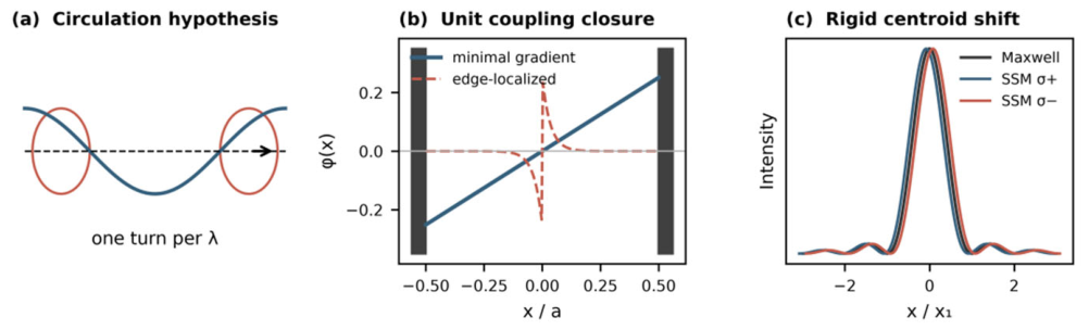
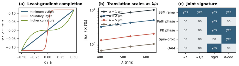
Figure 2.
Parameter dependence and discrimination. (a) Alternative phase completions illustrating why the closure must be stated explicitly. (b) Fractional translation Δx/x₁ as a function of wavelength and slit width under the unit-coupling closure. (c) Joint-signature matrix distinguishing the proposed SSM ramp from representative path-phase, Pancharatnam–Berry-phase, spin–orbit, and orbital-angular-momentum mechanisms; the matrix guides the design and is not an exhaustive classification.
Figure 2.
Parameter dependence and discrimination. (a) Alternative phase completions illustrating why the closure must be stated explicitly. (b) Fractional translation Δx/x₁ as a function of wavelength and slit width under the unit-coupling closure. (c) Joint-signature matrix distinguishing the proposed SSM ramp from representative path-phase, Pancharatnam–Berry-phase, spin–orbit, and orbital-angular-momentum mechanisms; the matrix guides the design and is not an exhaustive classification.
3. Joint Scaling and Falsification Criteria
A lateral displacement by itself would not establish circulation: static lens aberration, detector distortion, slit taper, beam walk, and polarization leakage can all move a centroid. The claim to be tested is the joint pattern—the displacement reverses between σ+ and σ−, vanishes for an equal helicity mixture, preserves the fringe geometry, and follows Crγ/a when wavelength and aperture vary.
We take the helicity-difference estimator D = (x̂+—x̂−)/2, for which the closure gives D = Cx₁rγ/a. A conventional path phase can translate a pattern but is not helicity odd; a geometric phase can be helicity odd but normally reshapes the phase topology instead of rigidly translating the single-slit envelope; spin–orbit coupling depends on helicity but carries a different aperture and wavelength dependence [16,17,18]. No single feature discriminates; the combination does. Supplement 1 (Section S6, Table S7) tabulates the same-geometry functional signatures of these alternatives against the closure.
For a laboratory claim we register eight kill criteria, stated fully in Supplement 1 (Section S6): K1, no helicity reversal; K2, failure of the fractional λ scaling; K3, failure of the inverse aperture scaling; K4, a non-rigid shape change; K5, a linear-polarization residual; K6, disagreement between the classical-light and heralded-single-photon channels; K7, reproduction by a material-resolved Maxwell model; K8, a joint signal whose fitted C departs from unity beyond the registered uncertainty. Any single failure rejects the unit-coupling SSM interpretation. One mechanism discriminator is registered alongside. D1 (thickness fork): a boundary-phase closure predicts a coupling independent of screen thickness d, whereas every transit-imprint mechanism predicts |C| ∝ d under the ceiling |C| ≤ 1.2776(d/h) (Supplement 1, Section S7). A thickness series from 60 nm to about 1 μm separates the two classes: at d ≈ 0.8–1 μm the transit class predicts |C| ≈ 1.0–1.3, while the boundary closure predicts C = 1 at every thickness. The asymmetry runs in a useful direction: thickness dependence falsifies the boundary-closure reading, and thickness independence at order-unity C excludes the transit class.
4. Maxwell-FDTD Null Control
The standard-optics control is essential. For a mirror-symmetric, reciprocal slit illuminated by a symmetric incident field, the linear Maxwell boundary-value problem preserves parity in the transverse coordinate. The far-field intensity obeys Iσ(q) = Iσ(−q) and the angular centroid vanishes; Supplement 1 gives the full symmetry and momentum bookkeeping. Transverse-momentum conservation says the same: a symmetric aperture transfers no net transverse momentum to a symmetric beam. A helicity label alone does not break mirror symmetry.
The parity argument and the FDTD control bound electromagnetic systematics; the exclusion analysis (Supplement 1, Section S7) bounds a disjoint class—medium-flow configurations that could imitate the boundary phase—through a theorem (quasi-static flows give exactly zero edge phase difference) and a ceiling (transit imprints reach at most 1.2776(d/h)). The two controls complement each other: Maxwell optics gives no signal, and no flow-based mechanism can fake an order-unity signal at the thicknesses used here.
To make the electromagnetic control computational, we solved the two-dimensional vector Maxwell equations on a Yee grid [19,20] for a slit in a perfect-electric-conductor screen, using the open-source fdtd package, version 0.5. The computational window measured 8 μm transverse by 3 μm longitudinal, with perfectly matched layers [21] of thickness 0.6 μm on all sides. A 120 nm PEC screen centred at z = 1.50 μm carried a centred slit of width a = 2 or 5 μm. A uniform soft line source at z = 0.90 μm drove either the x or the y electric-field component at λ = 633 nm; circular polarization was represented by summing the intensities of the two orthogonal solutions.
The grid spacing was 40, 20, or 10 nm, forming a factor-two refinement ladder. The solver supplied the Courant time step, and each run covered 1800 steps. We demodulated the last two optical cycles at the detector plane, zero-padded the complex field to 65,536 samples, and evaluated the angular spectrum for |θ| < 0.08 rad; the centroid came from the summed intensities of the two source polarizations. Since geometry and excitation are mirror symmetric, the continuum Maxwell centroid is exactly zero, and any finite value is read as a numerical residual.
The line source launches a cylindrical wave rather than a plane wave. The symmetry null requires only that the illumination be even about x = 0, which the centred line source satisfies exactly; a plane wave is the limiting case of zero wavefront curvature. A symmetric, softly focused laboratory beam shares this evenness, so the cylindrical-wave control stands closer to the proposed experiment than an idealized plane-wave control would.
Figure 3.
Maxwell-FDTD null control at λ = 633 nm. (a), (b) Total far-field intensity for 2 and 5 μm slits on a logarithmic scale; dashed lines mark the SSM C = 1 predictions, ±15.9429 and ±2.5509 mrad. (c) Absolute centroid residuals on the 40/20/10 nm refinement ladder (logarithmic scale): 0.09545, 0.04621, and 0.01338 mrad for the 2 μm slit, and 0.01965, 0.00111, and 0.00082 mrad (magnitudes plotted; the finest-grid 5 μm residual is negative) for the 5 μm slit. All finite values are numerical residuals, not a claimed physical displacement.
Figure 3.
Maxwell-FDTD null control at λ = 633 nm. (a), (b) Total far-field intensity for 2 and 5 μm slits on a logarithmic scale; dashed lines mark the SSM C = 1 predictions, ±15.9429 and ±2.5509 mrad. (c) Absolute centroid residuals on the 40/20/10 nm refinement ladder (logarithmic scale): 0.09545, 0.04621, and 0.01338 mrad for the 2 μm slit, and 0.01965, 0.00111, and 0.00082 mrad (magnitudes plotted; the finest-grid 5 μm residual is negative) for the 5 μm slit. All finite values are numerical residuals, not a claimed physical displacement.
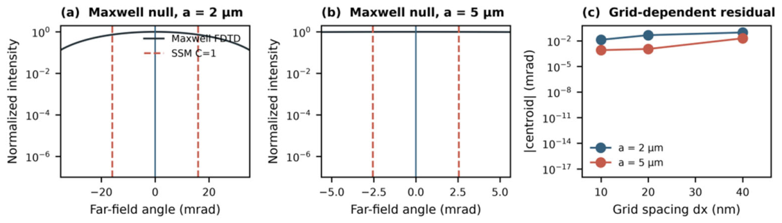
For the 2 μm slit the residual centroid falls monotonically along the ladder—0.0955, 0.0462, and 0.0134 mrad at 40, 20, and 10 nm—with reduction factors of 2.07 and 3.45 per halving, consistent with discretization error converging toward the symmetry-required zero. For the 5 μm slit the residuals (0.0196, 0.0011, and −0.0008 mrad) collapse to the discretization noise floor and change sign at the finest grid. Even the coarsest residual sits two orders of magnitude below the corresponding unit-coupling deflection (0.60% for the 2 μm slit and 0.77% for the 5 μm slit at 40 nm; 0.084% and 0.032% at 10 nm). The control is exact for the stated two-dimensional PEC geometry; it is not yet a three-dimensional, dispersive-material calculation, and a positive laboratory result would still require material-resolved modelling before any non-Maxwellian reading were entertained.
5. Pilot-Scale Numerical Validation
No laboratory raw frames were available for this study, so the one-wavelength, two-slit component appears as pilot-scale numerical validation of the measurement and analysis chain, not as a completed experiment. We generated synthetic photon-counting frames at λ = 633 nm and an effective focal length of 0.25 m for a = 2 and 5 μm, using an ideal Fraunhofer sinc² profile, 10⁶ detected photons per frame, 4 μm detector pixels, Poisson fluctuations, and Gaussian readout noise of 3 counts standard deviation. Two hundred realizations per condition were analysed with an iterative matched-filter (Fisher-scoring) translation estimator [22,23,24]. Starting from Δx⁽⁰⁾ = 0, six updates were applied:
For stability the step was limited to ±0.3x₁ per iteration. The reported coupling uncertainty is the standard deviation across independent realizations rather than the ideal Cramér–Rao bound. The pilot model omits real lens aberrations, imperfect polarization extinction, slit taper, surface roughness, and detector nonlinearity; Supplement 1 gives the full statistical model and settings.
Figure 4.
Pilot-scale numerical validation, not laboratory data. (a) One simulated photon-counting frame for the 2 μm slit with the SSM mean profile overlaid. (b) Coupling C recovered from 200 synthetic SSM realizations at each slit width; error bars give one standard deviation across realizations. (c) Bias of the same estimator on Maxwell-null synthetic frames; error bars give the standard error of the 200-realization mean.
Figure 4.
Pilot-scale numerical validation, not laboratory data. (a) One simulated photon-counting frame for the 2 μm slit with the SSM mean profile overlaid. (b) Coupling C recovered from 200 synthetic SSM realizations at each slit width; error bars give one standard deviation across realizations. (c) Bias of the same estimator on Maxwell-null synthetic frames; error bars give the standard error of the 200-realization mean.
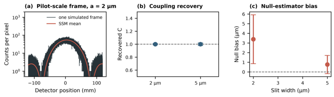
On SSM synthetic frames the recovered couplings are C = 1.000004 ± 0.009631 (a = 2 μm) and C = 1.000180 ± 0.019617 (a = 5 μm), with mean translations of 3.985744 and 0.637831 mm against inputs of 3.985727 and 0.637716 mm. On Maxwell-null frames the mean biases are 3.392 and 0.766 μm, with single-realization scatter of 35.831 and 13.385 μm. The estimator thus separates an order-unity synthetic closure from a null input under the stated idealized noise model; this says nothing yet about feasibility under real aberrations.
Two template-level checks support feasibility. First, the sinc² template neglects the obliquity (inclination) factor cos θ of the exact diffraction pattern. Repeating the estimation on noiseless obliquity-weighted frames returns shifts biased toward zero by only 44.2 μm (−1.11%) for a = 2 μm and 1.13 μm (−0.18%) for a = 5 μm: the mismatch shrinks a signal rather than fabricating one, and including the obliquity factor in the analysis template removes it outright (Supplement 1). Second, truncating the detector window to ±1.5 fringe spacings costs less than 18% of the Fisher information, so a standard camera sensor suffices (Supplement 1).
The photon budget is correspondingly modest. At 633 nm a 10⁶-photon frame (photon energy 3.14 × 10⁻¹⁹ J) accumulates in 0.31 μs at a detected power of 1 μW, in 0.31 s at 1 pW, and in 1 s on a heralded single-photon channel at 10⁶ detected counts per second. During a 1 ms exposure the mean power deposited on the detector is 3.14 × 10⁻¹⁰ W, far from the saturation or damage thresholds of silicon sensors (Supplement 1).
6. Discussion
The formulation here is narrower on purpose than a claim to have observed photon circulation. The theory is conditional: C = 1 follows only once the SSM unit-circulation edge normalization and the least-gradient completion are adopted. The numerics are limited as well—the Maxwell control is a two-dimensional PEC model and the pilot study uses synthetic frames—and neither is laboratory evidence.
Narrow as it is, the claim repairs the central logical defect of the earlier formulation. Without the closure a measured translation would determine only the product Crγ, and since rγ = λ/2π already belongs to the model, fitting C and rγ separately would be circular. With C fixed to unity by an explicit postulate, the experiment tests a definite boundary coupling together with its joint parameter dependence: a null result bounds or rejects the closure, while a positive result would motivate, though not by itself complete, a relativistic field-theoretic account.
The exclusion analysis also fixes what a completion must supply. The circulation–frequency product is set by spin quantization [Eq. (3)]; quasi-static medium flows give exactly zero edge phase difference; transit imprints fall an order of magnitude short at realistic thicknesses. What remains is an order-unity boundary phase coupling, and in the companion dynamics model [8] exactly one sector can carry it: the coupling between the Goldstone phase field, whose winding number is the helicity itself, and the medium displacement field. Deriving C then reduces to computing one dimensionless conversion efficiency whose target value is unity—a target made precise by the analysis of Supplement 1 (Section S7). A positive result at sub-micron thickness would select this channel by exclusion, and the thickness fork (D1, Section 3) tests that selection directly.
A convincing laboratory study should use at least two wavelengths and several slit widths, interchangeable helicity and linear-polarization states, reversed optical mounts, translated and rotated slits, achiral reference apertures, and material variants; both classical-light and heralded single-photon channels should be recorded [25,26]. The screen-thickness series—60, 120, and 240 nm films plus at least one thick (0.8–1 μm) screen—should run on the same apparatus so that the thickness fork is executed without extra optics. The analysis should be registered before unblinding, with centroid estimation cross-checked by full-pattern likelihood fitting, and any non-null claim should come with three-dimensional electromagnetic modelling using measured slit geometry and material constants.
A first test is inexpensive by design. Since Δx/x₁ = Cλ/(2πa) does not depend on focal length, the fringe scale can be matched to the sensor without touching the observable: a 50 mm lens puts the predicted C = 1 translation at 0.80 mm for a = 2 μm (0.13 mm for a = 5 μm), well within reach of a scientific CMOS camera with micrometre pixels. The remaining classical-channel hardware is a 633 nm helium–neon or diode laser, a zero-order half-wave plate or Fresnel rhomb for helicity switching, commercial vacuum-deposited slits of certified width, and a translation stage for the systematic checks. The photon budget shows that the classical channel needs no intensified or cryogenic detector, and the single-photon variant adds only a heralded source and a counting module of the kind standard in quantum-optics laboratories [25,26]. A decisive first experiment is therefore within the budget of an advanced undergraduate laboratory, and either outcome—a null bounding C or an order-unity helicity-odd translation—would be informative.
Table 1 collects the predicted unit-coupling translations for common laser wavelengths and both slit widths at f = 50 mm, together with the focal-length-independent fractional shift Δx/x₁ = λ/(2πa). Every absolute entry exceeds the centroid resolution of a standard scientific CMOS sensor by at least two orders of magnitude; the fractional columns are the registered observable of Section 2 and do not depend on the choice of lens, so a laboratory may adapt the geometry to its own camera without touching the prediction.
The registered minimal protocol is correspondingly short. (i) Illuminate the slit with a symmetric, softly focused beam; evenness about the slit centre, not plane-wave purity, is the symmetry requirement (Section 4). (ii) Switch the helicity with a zero-order half-wave plate or Fresnel rhomb in an interleaved σ+/σ−/linear sequence, logging the polarization extinction before and after each run. (iii) Record frames at f = 50 mm with a fiducial-grid calibration, interleaved dark frames, and slit translation and rotation runs for the controls catalogued in Supplement 1. (iv) Estimate the translations with the published matched-filter pipeline, form the helicity-difference estimator D, and apply the kill criteria K1–K8 to blinded data. (v) Execute the thickness fork D1 by repeating the identical sequence on 60, 120, and 240 nm films and on one thick (0.8–1 μm) screen. A second wavelength and a heralded single-photon channel are first upgrades, not prerequisites.
7. Conclusion
The unit-coupling SSM closure yields a sharp, falsifiable diffraction signature: a helicity-odd rigid translation with fractional shift Cλ/(2πa). Spin quantization fixes every factor except the dimensionless boundary coupling itself, which the closure pins to unity as an explicit, exposed postulate. Standard Maxwell electrodynamics returns a symmetry-protected null for the stated geometry, the two-dimensional controls show no competing order-unity displacement, and the exclusion analysis removes the full class of quasi-static and transit medium-flow mimicries at realistic screen thicknesses, leaving the registered thickness fork as the mechanism discriminator. The pilot study validates the estimation pipeline end to end on synthetic frames, the falsification criteria are fixed in advance, and the predicted signals sit two orders of magnitude above the reach of ordinary laboratory cameras. The question—does the photon carry a transverse circulation?—is now one that a modest laboratory can answer, and we invite independent groups to put it to the test.
Disclosures
The authors declare no conflicts of interest.
Data availability
Data underlying the results presented in this paper are contained in the files fdtd_results.npz, pilot_results.json, pilot_robustness.json, simulation_summary.json, and exclusion_analysis.py (the boundary-value and transit-imprint calculations of Supplement 1, Section S7), which are available from the corresponding author upon reasonable request. No laboratory experimental data were generated or analysed for this study.
Supplemental document
See Supplement 1 for supporting content, including the conditional derivation of the unit-coupling closure, the Maxwell symmetry and momentum bookkeeping, the FDTD implementation tables, the estimator equations, the boundary-coupling exclusion analysis and the thickness fork, the laboratory controls and kill criteria, and the reproducibility files.
Funding
This research did not receive any specific grant from funding agencies in the public, commercial, or not-for-profit sectors.
Acknowledgments
The authors thank the developers of the open numerical tools used for the verification calculations.
References
- Glauber, R. J. The quantum theory of optical coherence. Phys. Rev. 1963, 130, 2529–2539. [Google Scholar] [CrossRef]
- Taylor, G. I. Interference fringes with feeble light. Proc. Camb. Philos. Soc. 1909, 15, 114–115. [Google Scholar]
- Grangier, P.; Roger, G.; Aspect, A. Experimental evidence for a photon anticorrelation effect on a beam splitter: a new light on single-photon interferences. Europhys. Lett. 1986, 1, 173–179. [Google Scholar] [CrossRef]
- Hawton, M. Photon position operator with commuting components. Phys. Rev. A 1999, 59, 954–959. [Google Scholar] [CrossRef]
- Bohm, D. A suggested interpretation of the quantum theory in terms of ‘hidden’ variables. I. Phys. Rev. 1952, 85, 166–179. [Google Scholar] [CrossRef]
- Cheng, J.; Cheng, D. The spiral structure model: a geometric phenomenology of wave-particle duality, spin, and electromagnetic coupling. Preprints 2026. [Google Scholar] [CrossRef]
- Cheng, J.; Cheng, D. The natural philosophical nature of light: a hypothesis of energetic mass points in uniform spiral linear motion in space. Preprints 2026. [Google Scholar] [CrossRef]
- Cheng, J.; Cheng, D. Toward the dynamics of the spiral structure model: canonical quantization, core electrodynamics, and the defect propagator. Preprints 2026. [Google Scholar] [CrossRef]
- Einstein. Über einen die Erzeugung und Verwandlung des Lichtes betreffende heuristische Gesichtspunkt. Ann. Phys. 1905, 322, 132–148. [Google Scholar] [CrossRef]
- Compton, H. A quantum theory of the scattering of X-rays by light elements. Phys. Rev. 1923, 21, 483–502. [Google Scholar] [CrossRef]
- Beth, R. A. Mechanical detection and measurement of the angular momentum of light. Phys. Rev. 1936, 50, 115–125. [Google Scholar] [CrossRef]
- Goodman, J. W. Introduction to Fourier Optics, 3rd ed.; Roberts, Ed.; 2005. [Google Scholar]
- P. G. Saffman, Vortex Dynamics; Cambridge University Press, 1992.
- Leonhardt, U.; Piwnicki, P. Optics of nonuniformly moving media. Phys. Rev. A 1999, 60, 4301–4312. [Google Scholar] [CrossRef]
- G. E. Volovik, The Universe in a Helium Droplet; Clarendon Press, 2003.
- Pancharatnam, S. Generalized theory of interference, and its applications. Part I. Coherent pencils. Proc. Indian Acad. Sci. A 1956, 44, 247–262. [Google Scholar]
- Berry, M. V. Quantal phase factors accompanying adiabatic changes. Proc. R. Soc. Lond. Ser. A 1984, 392, 45–57. [Google Scholar] [CrossRef]
- Sztul, H. I.; Alfano, R. R. Double-slit interference with Laguerre–Gaussian beams. Opt. Lett. 2006, 31, 999–1001. [Google Scholar] [CrossRef] [PubMed]
- Yee, K. S. Numerical solution of initial boundary value problems involving Maxwell’s equations in isotropic media. IEEE Trans. Antennas Propag. 1966, 14, 302–307. [Google Scholar] [CrossRef]
- Taflove; Hagness, S. C. Computational Electrodynamics: The Finite-Difference Time-Domain Method, 3rd ed.; Artech House, 2005. [Google Scholar]
- Berenger, J.-P. A perfectly matched layer for the absorption of electromagnetic waves. J. Comput. Phys. 1994, 114, 185–200. [Google Scholar] [CrossRef]
- Giovannetti, V.; Lloyd, S.; Maccone, L. Quantum-enhanced measurements: beating the standard quantum limit. Science 2004, 306, 1330–1336. [Google Scholar] [CrossRef] [PubMed]
- Caves, M. Quantum-mechanical noise in an interferometer. Phys. Rev. D. 1981, 23, 1693–1708. [Google Scholar] [CrossRef]
- Kay, S. M. Fundamentals of Statistical Signal Processing: Estimation Theory; Prentice Hall, 1993. [Google Scholar]
- Hadfield, R. H. Single-photon detectors for optical quantum information applications. Nat. Photonics 2009, 3, 696–705. [Google Scholar] [CrossRef]
- Eisaman, M. D.; Fan, J.; Migdall, A.; Polyakov, S. V. Invited review article: single-photon sources and detectors. Rev. Sci. Instrum. 2011, 82, 071101. [Google Scholar] [CrossRef] [PubMed]

Table 1.
Predicted unit-coupling (C = 1) translations at f = 50 mm and the focal-length-independent fractional shifts. The fractional shift is the registered observable; the absolute translation sets the detector requirement.
Table 1.
Predicted unit-coupling (C = 1) translations at f = 50 mm and the focal-length-independent fractional shifts. The fractional shift is the registered observable; the absolute translation sets the detector requirement.
| λ (nm) | Δx, a = 2 μm (mm) | Δx/x₁, a = 2 μm | Δx, a = 5 μm (mm) | Δx/x₁, a = 5 μm |
|---|---|---|---|---|
| 405 | 0.326 | 0.0322 | 0.052 | 0.0129 |
| 532 | 0.563 | 0.0423 | 0.090 | 0.0169 |
| 633 | 0.797 | 0.0504 | 0.128 | 0.0202 |
| 850 | 1.438 | 0.0677 | 0.230 | 0.0271 |
| 1550 | 4.781 | 0.1234 | 0.765 | 0.0493 |
Disclaimer/Publisher’s Note: The statements, opinions and data contained in all publications are solely those of the individual author(s) and contributor(s) and not of MDPI and/or the editor(s). MDPI and/or the editor(s) disclaim responsibility for any injury to people or property resulting from any ideas, methods, instructions or products referred to in the content. |
© 2026 by the authors. Licensee MDPI, Basel, Switzerland. This article is an open access article distributed under the terms and conditions of the Creative Commons Attribution (CC BY) license (http://creativecommons.org/licenses/by/4.0/).
Copyright: This open access article is published under a Creative Commons CC BY 4.0 license, which permit the free download, distribution, and reuse, provided that the author and preprint are cited in any reuse.