How Deep Is the Control? A Parallel-Parking Story of Lie-Bracket Depth–Width Trade-Offs, the Generic Bias of Learned Models, and a Negative Result on Structural Priors

1. Introduction: The Car That Cannot Slide

1.1. The Question

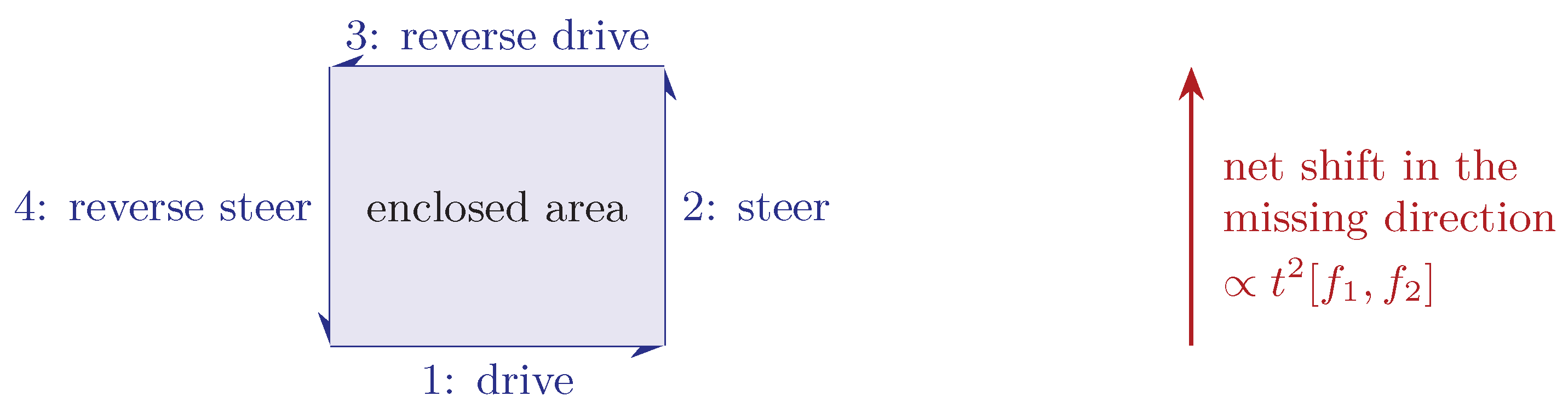
A car has two controls. You can drive forward or backward, and you can steer. It lives in three dimensions: position along the street, position across the street, and heading. Nothing in the controls moves the car sideways, and yet every driver parallel-parks. The sideways motion is not given; it is built by composing the two controls in time: forward with the wheel turned, back with the wheel turned the other way, and so on. The net result is a small sideways displacement, and it is bought with time: the smaller the displacement per manoeuvre, the more manoeuvres you need.

Mathematically this is a Lie bracket. Chow–Rashevskii theory says that a few vector fields can reach a high-dimensional space if their Lie brackets span it [1,2,3]. A bracket of nesting depth $\delta$ is paid for in time: it enters the flow at order $t^{\delta +1}$, which is the content of the ball–box picture [6,7,8]. So there is a currency exchange between width (number of channels) and depth (temporal composition).

Figure 1. The mechanism of the paper in one picture (Heisenberg-type system). The four moves return the planar position to its start, but the third coordinate gains the enclosed area: a displacement of order $t^2$ along $[f_1,f_2]$, a direction neither control supplies. A bracket of depth k needs $3·2^k-2$ such segments and gives displacement of order $t^{k+1}$.

Figure 1. The mechanism of the paper in one picture (Heisenberg-type system). The four moves return the planar position to its start, but the third coordinate gains the enclosed area: a displacement of order $t^2$ along $[f_1,f_2]$, a direction neither control supplies. A bracket of depth k needs $3·2^k-2$ such segments and gives displacement of order $t^{k+1}$.

This paper starts from that exchange and asks three questions that get progressively harder:

Q1. 

Algebra. For d state dimensions and r generating fields, how deep must brackets go, and is that ever too pessimistic?

Q2. 

Physics. If the controller is noisy, how much depth is actually usable, and what does feedback buy?

Q3. 

Learning. If we fit a control-affine model to trajectories and compute the bracket depth of the fitted model, do we learn the depth of the true system?

Q1 and Q2 turn out to have clean answers. Q3 does not, and most of the paper is an account of why.

1.2. Overview: The Story in Five Acts

The paper follows one thread: depth is a loan taken out in time. Each part asks what the loan costs, who can repay it, and whether a learner can tell that it was taken.

• Act I (§3): the price list. Counting gives a lower bound on how many nested manoeuvres are needed, tightness shows it cannot be improved in general, and a pair of examples shows no upper bound exists.
• Act II (§4): the typical car. A genericity theorem predicts that a “random” system sits exactly at the counting bound. That is the sentence the rest of the paper tests.
• Act III (§5–§8): the physics works. On designed systems, time scaling and the noise law behave as theory says, and we are clear about which constants are protocol-dependent.
• Act IV (§9–§11): the witness that cannot testify. Fitted models hit the counting bound, not the truth, unless the model class contains the truth. Real data and world models give a fitted depth that equals the generic bound and also equals the null, so we cannot yet claim to have seen structure in the brain or in a JEPA.
• Act V (§12): bribing the witness. A gradient-level prior meant to push depth upward fails; we re-read the loss and find the failure is at least partly of our own making.

Table 1. Parking dictionary: how each everyday idea maps to a statement in the paper.

Parking story	Mathematics	Where
Two controls, three dimensions	r generating fields, d state dimensions	§2
Sideways motion built from drive and steer	Lie bracket $[f,g]=Dgf-Dfg$	§2
Number of nested manoeuvres	Nesting depth, counted by ${\delta }_{\mathrm{LB}}(d,r)$	§3
A car whose steering makes every extra dimension cost one more manoeuvre	Filiform system, depth $d-2$	Prop. 1
A random car	Generic polynomial system	Thm. 3
Smaller shift per manoeuvre	Displacement $t^{k+1}B\left(p\right)$	Prop. 2
Hand tremor	Timing, amplitude, state noise	§5,§8.1
Looking where you are between moves	Feedback, state reset	§8.2
Watching someone park and guessing how many manoeuvres it took	Depth of a fitted model	§9
Asking the observer to find longer manoeuvres than it can express	Bracket-injector prior	§12

Table 1. Parking dictionary: how each everyday idea maps to a statement in the paper.

Parking story	Mathematics	Where
Two controls, three dimensions	r generating fields, d state dimensions	§2
Sideways motion built from drive and steer	Lie bracket $[f,g]=Dgf-Dfg$	§2
Number of nested manoeuvres	Nesting depth, counted by ${\delta }_{\mathrm{LB}}(d,r)$	§3
A car whose steering makes every extra dimension cost one more manoeuvre	Filiform system, depth $d-2$	Prop. 1
A random car	Generic polynomial system	Thm. 3
Smaller shift per manoeuvre	Displacement $t^{k+1}B\left(p\right)$	Prop. 2
Hand tremor	Timing, amplitude, state noise	§5,§8.1
Looking where you are between moves	Feedback, state reset	§8.2
Watching someone park and guessing how many manoeuvres it took	Depth of a fitted model	§9
Asking the observer to find longer manoeuvres than it can express	Bracket-injector prior	§12

1.3. What This Paper Does and Does Not Claim

Every statement carries a status tag: [classical] known mathematics restated; [proved] proved here; [proved, conditional] proved under stated hypotheses we have not removed; [heuristic] argument without proof; [measured] an experimental result as stated; [inconclusive] a pre-registered gate that could not separate signal from null; [not met] a gate that was not met; [open] unresolved.

We do claim: the counting bound and its tightness (classical); generic attainment in polynomial families (new, proved); a measured agreement between designed-system experiments and the theory; and a negative result about learned depth estimates and the bracket-injector.

We do not claim: that learned models in general sit at ${\delta }_{\mathrm{LB}}$ (that is Conjecture 1, open); that real neural or world-model data have no Lie structure beyond the generic bound (our test cannot tell); that the noise constant c is universal (it is not, across our protocols); or that no gradient-level prior can ever work.

1.4. Contributions, Ranked by How Firmly They Stand

• [proved] Generic depth attainment (Thm. 3) with a proof in which the lower bound is deterministic; only attainment is generic.
• [classical]+[proved] Exact counting bound, tightness, and a pair of linear-depth examples (Thms. 1, 2, Prop. 1).
• [measured] Time scaling and noise law on designed systems; the noise slope depends on segment duration and we give a heuristic that predicts that dependence (§5, §8).
• [measured] On four testbeds, pure neural fits sit at ${\delta }_{\mathrm{LB}}$ and bilinear fits succeed only inside their class (§9).
• [inconclusive] Four real ALM sessions (§11); [measured] $d_{\mathrm{eff}}$ only for H-JEPA (§11.2).
• [not met] Bracket-injector, with a corrected analysis of why (§12).

2. Setting and Conventions

Let M be a smooth d-manifold and consider

$$\dot{x}=f_0\left(x\right)+{\displaystyle \sum _{i=1}^m}{u}_i\left(t\right)f_i\left(x\right),u_i\left(t\right)\in U\subset \mathbb{R},$$

(1)

with $f_0$ the drift. Write $r=m+1$ for the number of generating fields and use the bracket $[f,g]=Dgf-Dfg$.

Definition 1

(Nesting depth). Generators have depth 0. A bracket $[f_i,B]$ with B of depth $\delta -1$ and $i\in \{0,\dots ,m\}$ has depth δ. Let ${\mathfrak{L}}_{\delta }\left(p\right)\subset T_{p}M$ be the span of the values at p of all brackets of depth $\le \delta$, and ${\mathrm{depth}}_p=\min \{\delta :{\mathfrak{L}}_{\delta }\left(p\right)=T_{p}M\}$.

Definition 2

(Counting quantities). Witt’s formula gives the dimension of the degree-j part of the free Lie algebra on r generators:

$$L(r,j)={\displaystyle \frac{1}{j}}\sum _{e\mid j}\mu \left(e\right)r^{j/e},$$

(2)

with μ the Möbius function. Put $N_r\left(w\right)={\sum }_{j=1}^{w}L(r,j)$ and

$${\delta }_{\mathrm{LB}}(d,r)=\min \{\delta \ge 0:N_r(\delta +1)\ge d\}.$$

(3)

Definition 3

(Accessibility, LARC). System (1) satisfies the Lie algebra rank condition (LARC) at p if ${\mathrm{depth}}_p<\infty$. LARC implies accessibility [3]; with drift or one-sided inputs it does not imply controllability.

Remark 1

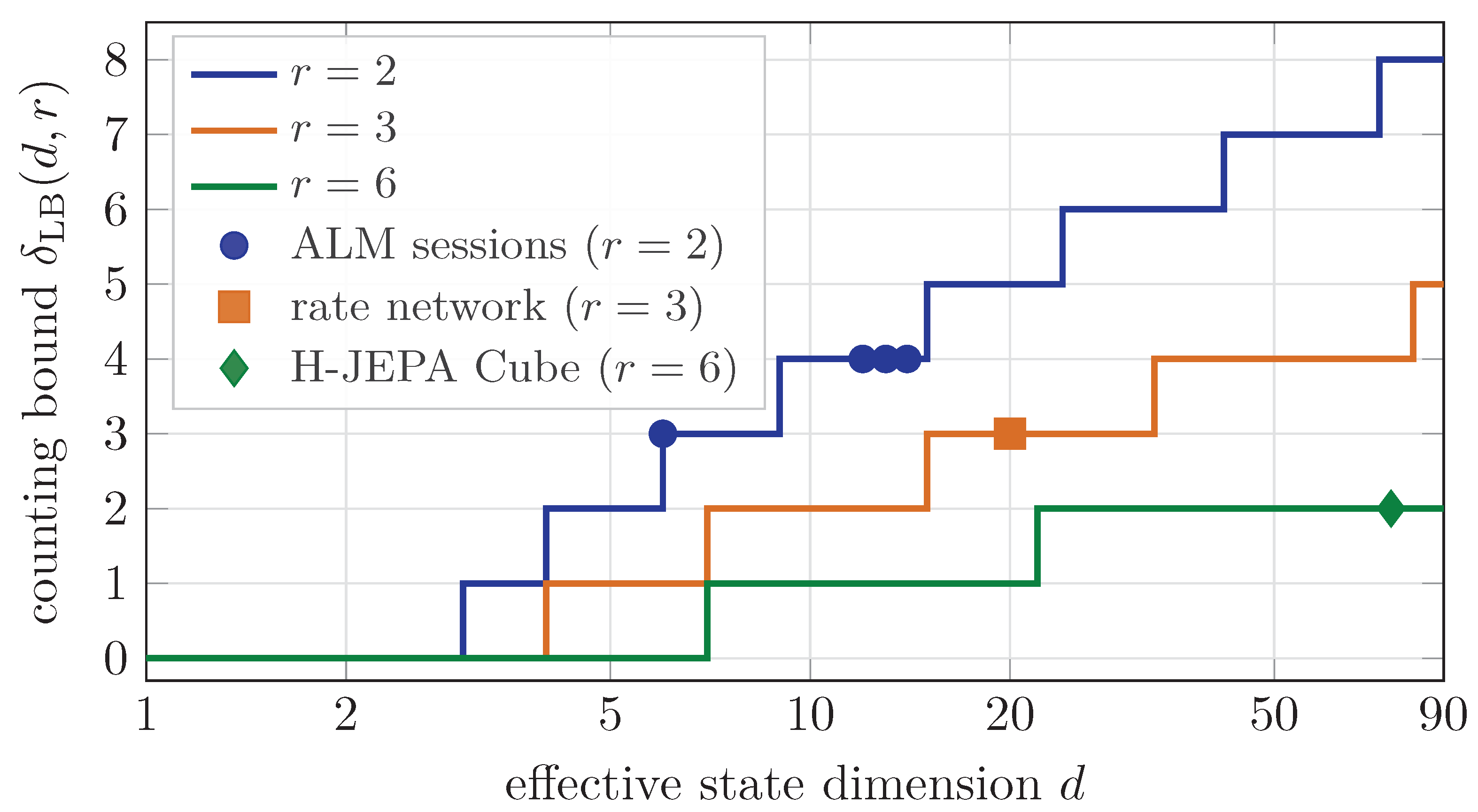
(${\delta }_{\mathrm{LB}}$ is a staircase). ${\delta }_{\mathrm{LB}}(d,r)$ changes only when d crosses a value $N_r\left(w\right)$. For $r=2$ the thresholds are $2,3,5,8,14,23,41,71,\dots$; for $r=3$ they are $3,6,14,32,80,\dots$; for $r=6$, $6,21,91,\dots$. A fitted model whose effective dimension is uncertain by a few units therefore usually has an unambiguous ${\delta }_{\mathrm{LB}}$, which is what makes it a usable prediction (Figure 2).

A bookkeeping convention that matters later. The r in ${\delta }_{\mathrm{LB}}(d,r)$ is the number of generating fields of the object whose depth is being computed. For a designed testbed this may be two driftless fields; for a fitted control-affine model with $m=2$ inputs and a drift it is 3. The same testbed can therefore have a true depth above the ${\delta }_{\mathrm{LB}}$ of its fitted model (Appendix B).

3. Act I — The Price List: What the Algebra Allows

Theorem 1

(Counting lower bound and width form). [classical] Let $r\ge 2$ fields be given on a d-manifold. For all p and δ, $\dim {\mathfrak{L}}_{\delta }\left(p\right)\le \min \{d,N_r(\delta +1)\}$. Hence if LARC holds at p with depth δ, then $\delta \ge {\delta }_{\mathrm{LB}}(d,r)$ and $r\ge {(d/2)}^{1/(\delta +1)}$.

Proof. 

Brackets of depth $\le \delta$ lie in the span of Lie monomials of length $\le \delta +1$ in r letters. By Witt’s theorem their number of independent elements is at most $N_r(\delta +1)$, and evaluation at p cannot increase rank. For the width form, $L(r,j)\le r^j/j\le r^j$ gives $N_r\left(w\right)\le r(r^w-1)/(r-1)\le 2r^w$ for $r\ge 2$, so $d\le 2r^{\delta +1}$.    □

Remark 2

(Asymptotics). $N_r\left(w\right)=(1+o\left(1\right)){\displaystyle \frac{r}{r-1}}{\displaystyle \frac{r^w}{w}}$, so ${\delta }_{\mathrm{LB}}(d,r)={\log }_{r}d+O\left(\log \log d\right)-1$. Depth is logarithmic in d at best: adding dimensions is cheap, adding channels is cheaper still.

Theorem 2

(Tightness). [classical] For every $r\ge 2$ and $d>r$ there is a driftless system of r left-invariant fields on a simply connected nilpotent Lie group of dimension d that satisfies LARC everywhere and reaches rank d at depth exactly ${\delta }_{\mathrm{LB}}(d,r)$.

Proof. 

Let $s={\delta }_{\mathrm{LB}}+1$ and let $\mathfrak{n}$ be the free nilpotent Lie algebra of step s on r generators, so $\dim \mathfrak{n}=N_r\left(s\right)\ge d>N_r(s-1)$. Since the top layer ${\mathfrak{n}}_s$ is central, every subspace of it is an ideal; choose one, I, of dimension $N_r\left(s\right)-d\le L(r,s)$ and set $\mathfrak{g}=\mathfrak{n}/I$. The r generators still generate $\mathfrak{g}$, $\dim {\mathfrak{L}}_{s-2}\le N_r(s-1)<d$, and $\dim {\mathfrak{L}}_{s-1}=d$.    □

Theorems 1 and 2 are, in substance, facts about free nilpotent Lie algebras [4,5]; we state them because the rest of the paper uses ${\delta }_{\mathrm{LB}}$ as a yardstick.

Proposition 1

(There is no universal upper bound). [proved]

(a) 

Filiform.On ${\mathbb{R}}^d$ let $X={\partial }_1$ and $Y={\partial }_2+{\sum }_{j=1}^{d-2}{\displaystyle \frac{x_1^j}{j!}}{\partial }_{j+2}$. This pair satisfies LARC everywhere and reaches rank d at depth exactly $d-2$.

(b) 

Single-input affine.For $\dot{x}=Ax+bu$ the depth is $\ge d-2$ for every $(A,b)$.

Proof. (a) By induction ${\mathrm{ad}}_X^{j}Y={\sum }_{i\ge j}{\displaystyle \frac{x_1^{i-j}}{(i-j)!}}{\partial }_{i+2}$. The matrix with rows $X,Y,{\mathrm{ad}}_{X}Y,\dots ,{\mathrm{ad}}_X^{d-2}Y$ is triangular with unit diagonal in the coordinates $({\partial }_1,\dots ,{\partial }_d)$, hence of full rank at every point, and ${\partial }_d$ appears only in ${\mathrm{ad}}_X^{d-2}Y$, so depth $d-2$ is needed. (b) With $f_0=Ax$ and $f_1=b$, brackets with the constant field b of any constant field vanish and $[f_0,c]=-Ac$ for constant c. The nonzero left-nested brackets are $f_0$, b and $\pm A^{j}b$. At depth $\delta$ their values span at most $\delta +2$ dimensions at p, so $\delta \ge d-2$.    □

The moral is a gap: with $r=2$ the counting bound is logarithmic in d while Prop. 1 gives depth linear in d. Anything between the two is possible, and which one a given system occupies is a structural fact, not a counting fact.

Proposition 2

(Time cost, driftless, signed inputs). [classical] For a depth-k bracket B, a nested group-commutator protocol of $n_k=3·2^k-2$ constant-control segments of duration t produces displacement $t^{k+1}B\left(p\right)+O\left(t^{k+2}\right)$.

The proof is a Baker–Campbell–Hausdorff induction and is in Appendix A.1. With a drift, pure $f_i$ flows are not available and reversed flows require signed inputs, so quantitative statements for one-sided inputs remain open [open].

4. Act II — The Typical Car: Random Systems Sit at the Bound

4.1. The Genericity Theorem

Theorem 1 says depth is at least ${\delta }_{\mathrm{LB}}$. The natural next question is when equality holds. It holds, in a precise sense, for almost every system.

Theorem 3

(Generic depth attainment). [proved] Fix $d,m\ge 1$, $r=m+1$, $s={\delta }_{\mathrm{LB}}(d,r)+1$ and a degree $D\ge s-1$. Let ${\mathcal{F}}_D$ be the finite-dimensional space of r-tuples of polynomial vector fields on ${\mathbb{R}}^d$ with coefficients of degree $\le D$ (in x), and let μ be a probability measure on ${\mathcal{F}}_D$, absolutely continuous with respect to Lebesgue measure on the coefficients. Then for μ-almost every tuple and Lebesgue-almost every $p\in {\mathbb{R}}^d$,

$${\mathrm{depth}}_p(f_0,\dots ,f_m)={\delta }_{\mathrm{LB}}(d,r).$$

Proof. 

Lower bound (deterministic). For $\delta <{\delta }_{\mathrm{LB}}$, $N_r(\delta +1)<d$, so by Theorem 1 the rank at depth $\delta$ is $<d$ at every tuple and every point.

A witness. Let $\mathfrak{g}$ be the nilpotent Lie algebra of Theorem 2 with its r generators. In exponential coordinates on the corresponding simply connected group, left-invariant fields are polynomial of degree at most $(\mathrm{step}-1)=s-1\le D$, because the Baker–Campbell–Hausdorff series terminates. This gives a tuple $f^{★}\in {\mathcal{F}}_D$ whose depth-${\delta }_{\mathrm{LB}}$ brackets span ${\mathbb{R}}^d$ at every point.

Algebraic genericity. Collect, for all left-normed words of length $\le s$ over the r generators, the values $B_w(f,p)\in {\mathbb{R}}^d$; the entries are polynomials in the coefficients c of f and in p. Some $d\times d$ minor $\Delta (c,p)$ of the matrix of these vectors is a polynomial that does not vanish at $(f^{★},p)$, so it is not identically zero. Its zero set has Lebesgue measure zero in $(c,p)$-space. Since $\mu \otimes \mathrm{Leb}$ is absolutely continuous, Fubini gives the statement for $\mu$-a.e. tuple and Leb-a.e. p. Together with the lower bound this shows depth is exactly ${\delta }_{\mathrm{LB}}$.    □

Remark 3

(Scope). The theorem is stated for a finite-dimensional polynomial family, where “absolutely continuous” is meaningful; spaces of $C^k$ fields carry no Lebesgue measure. It says nothing directly about non-polynomial classes such as neural networks, which is where we need it. That gap is the next statement.

4.2. From Polynomials to Learned Models

Corollary 1

(Learned models as generic draws). [heuristic] If a control-affine model is fitted by an objective with no term that favours structurally degenerate fields, and if the fitted model behaves like a typical draw from its function class, then its depth at generic reference points is ${\delta }_{\mathrm{LB}}(d_{\mathrm{eff}},m+1)$, where $d_{\mathrm{eff}}$ is the effective dimension of the model class restricted to the data distribution.

Figure 2. The counting bound ${\delta }_{\mathrm{LB}}(d,r)$ is a staircase in d (Remark 1). Markers show where the empirical systems of §10–§11.2 sit; testbed r values are listed in Appendix B. A few units of uncertainty in $d_{\mathrm{eff}}$ rarely change ${\delta }_{\mathrm{LB}}$.

Figure 2. The counting bound ${\delta }_{\mathrm{LB}}(d,r)$ is a staircase in d (Remark 1). Markers show where the empirical systems of §10–§11.2 sit; testbed r values are listed in Appendix B. A few units of uncertainty in $d_{\mathrm{eff}}$ rarely change ${\delta }_{\mathrm{LB}}$.

This is a prediction, not a theorem. Its rigorous form is:

Conjecture 1

(SGD concentrates at the counting bound). [open] Let $\mathcal{F}$ be a smooth class of control-affine fields, trained by SGD on a reconstruction loss from trajectories of a control-affine system, with no regulariser that penalises bracket structure. Then the iterates have depth ${\delta }_{\mathrm{LB}}(d_{\mathrm{eff}},m+1)$ at generic p with probability tending to one.

Two caveats belong next to this prediction rather than in an appendix. First, $d_{\mathrm{eff}}$ is usually a PCA dimension at a variance threshold, so it carries a threshold choice. The staircase structure of Remark 1 softens this. Second, a depth estimator applies a rank threshold, so “fitted depth $={\delta }_{\mathrm{LB}}$” is a joint statement about the model and the estimator. We return to both in §9.

4.3. Additive Control: What We Can and Cannot Say

The simplest control structure is additive input, $B\left(x\right)=B$ constant. Here the algebra is explicit.

Proposition 3

(Brackets for additive control). [proved] Let $\dot{x}=f_0\left(x\right)+{\sum }_i{u}_i{b}_i$ with constant $b_i$, $J\left(x\right)=D{f}_0\left(x\right)$, and $g_k^{\left(j\right)}={\mathrm{ad}}_{f_0}^j{b}_k$.

(a) 

$[f_0,b_k]=-J{b}_k$ and $[b_i,[f_0,b_k]]=-{\partial }^2{f}_0(b_i,b_k)$ (a Hessian bracket). In particular $[b_i,b_k]=0$.

(b) 

If $f_0$ is affine, or if $f_0\left(p\right)=0$, then $g_k^{\left(j\right)}\left(p\right)={(-J\left(p\right))}^j{b}_k$ for all j.

(c) 

Consequently, at such p, ${\mathfrak{L}}_{\delta }\left(p\right)\supseteq \mathrm{span}\{J^j{b}_k:j\le \delta \}$, so ${\mathrm{depth}}_p\le k_K(J\left(p\right),B)$, the Krylov index. For affine $f_0$, ${\mathfrak{L}}_{\delta }\left(p\right)=\mathrm{span}\{f_0\left(p\right),J^j{b}_k:j\le \delta \}$ and depth equals the Krylov index up to the single direction $f_0\left(p\right)$.

(Proof in Appendix A.2.)

Two readings are worth keeping apart. For affine $f_0$ this recovers the classical Kalman picture and Prop. 1(b): the Krylov index is the depth. For nonlinear $f_0$, the Krylov index is an upper bound at equilibria, and Hessian brackets (a) add up to $m(m+1)/2$ further directions per level that the linear picture does not have. So nonlinear drift with additive input can reach full rank sooner than the Krylov index suggests. Whether it reaches ${\delta }_{\mathrm{LB}}$ is not settled by any argument we have; (a) is only the reason to expect it can go below the Krylov index.

Proposition 4

(State-dependent input: conditional statement). [proved, conditional] Let $B_i\left(x\right)=D\left(x\right)b_i$ with $D\left(x\right)=\mathrm{diag}(1+\beta \tanh x_k)$, $\beta >0$, so that $[B_i,B_j]\not\equiv 0$. Level-one brackets then contribute at most $m(m+1)/2$ independent directions in total (the m drift brackets plus $\left({\displaystyle \genfrac{}{}{0pt}{}{m}{2}}\right)$ input–input brackets) and generically attain this; at higher levels the count is bounded by $N_{m+1}(\delta +1)$. Whether depth equals ${\delta }_{\mathrm{LB}}(d,m+1)$ for generic $f_0$ requires exhibiting one member of this family with full rank at depth ${\delta }_{\mathrm{LB}}$ (then the analytic-minor argument of Theorem 3 applies); we have not exhibited such a witness.

5. Act III — The Physics: What Noise Does to Depth

An open-loop protocol exploiting a depth-k direction cancels first-order displacements across $n_k=3·2^k-2$ segments. If each segment has an independent relative timing error of size $ϵ$, the first-order residuals add like $ϵt\sqrt{n_k}$, against a signal of order $t^{k+1}$.

A heuristic that predicts the slope. [heuristic] Requiring signal ≳ residual, $t^k\gtrsim ϵ\sqrt{3}{2}^{k/2}$. Taking logarithms with $L=\ln (1/t)$,

$$k_{\max }\left(ϵ\right)\approx {\displaystyle \frac{\ln (1/ϵ)-\frac{1}{2}\ln 3}{L+\frac{1}{2}\ln 2}},c\left(t\right)={\displaystyle \frac{1}{\ln (1/t)+\frac{1}{2}\ln 2}}.$$

(4)

This ignores bracket-magnitude and factorial prefactors, which shift $k_{\max }$ by $O\left(1\right)$ but would alter the slope if they grew superlinearly in k. The prediction is that c is not a constant: it depends on segment duration and is larger for larger t. We compare it with measurements in §8.1.

Conjecture 2

(Noise-limited depth). [open]  For open-loop piecewise-constant protocols built from nested group commutators, $k_{\max }\left(ϵ\right)=c\ln (1/ϵ)+O\left(1\right)$ with $c=c(t,\mathrm{protocol})>0$, and (4) describes the dependence of c on segment duration. Whether the $O\left(1\right)$ term and the residual protocol-dependence admit a clean description is open.

6. Experimental Protocol and How to Read It

All experiments follow a pre-registered protocol (phase0_frozen.json, hash 4296acbee635) with thresholds and seeds frozen before measurement, and BASE_SEED $=20261018$. Controls are signed, $u\in [-1,1]$, unless stated; sensitivities are computed by forward Jacobians at $\mathrm{rtol}={10}^{-10}$; rank thresholds are ${10}^{-7}$ (primary) and ${10}^{-10}$ (secondary); $n=5$ seeds unless noted; $95\%$ bootstrap intervals; Holm correction.

Testbeds. Heisenberg $d=3,5,6$; Engel $d=4,5$; Cartan $d=5$; Filiform $d=5$–9; KalmanChain $d=6,8$; generic bilinear $d=8,10,16$ with $r\in \{2,3\}$ generators.

Gates. A pre-registered gate is a pass/fail criterion stated before the run. A failed gate is reported as failed, with the numbers, not repackaged. Outcomes: P1 passed; P2 passed; P3 failed ($2/4<90\%$); P4 inconclusive (fitted CI overlaps null); P5 partial; injector Gate 3 failed.

Two cautions on sample size. The learning experiments use four testbeds (P3), four sessions (P4) and nine checkpoints measured only for $d_{\mathrm{eff}}$ (P5). These are existence checks, not statistical estimates of how learned models behave in general.

7. Act III, Continued — The Physics Works on Designed Systems

7.1. P1: Accessibility Under One-Sided Inputs

Question. With $u\in [0,1]$ only, does the endpoint map still have full rank?

Method. 16 systems, $u\in {[0,1]}^{N\times m}$, $N\in \{d,2d,4d,8d\}$; endpoint-map Jacobian by forward sensitivity; rank by relative SVD.

Result. [measured] All 16 systems reach full rank at $N\le 8d$; 15 of 16 at both thresholds. The bilinear $d=16$, $r=2$ system is tolerance-unstable (rank 13 at ${10}^{-7}$, rank 16 at ${10}^{-10}$, ${\sigma }_{\min }=1.86\times {10}^{-10}$), as expected from bracket suppression under one-sided inputs. Gate: passed. This is a numerical accessibility statement, not a proof; quantitative one-sided bounds remain open.

7.2. P1: Time Scaling

Question. Does ${\sigma }_{\min }$ of the endpoint map scale as $T^{k+1}$ for a system of depth k?

Result. [measured] Seven structured testbeds match the theory to within $0.02$ with $R^2=1.000$. The Filiform $d=9$ entry is checked by a constant ratio rather than a slope. The two generic bilinear systems deviate by $0.26$–$0.44$ and are consistent with not yet being in the asymptotic small-T regime. Gate: passed.

Table 2. Fitted exponent of ${\sigma }_{\min }\left(T\right)$ versus theory $k+1$.

System	k	Theory	Fit	${\mathit{R}}^2$	$\left|\mathit{\Delta }\right|$
Heisenberg $d=5$	1	2	1.989	1.000	0.011
Engel $d=5$	2	3	2.993	1.000	0.007
Cartan $d=5$	2	3	3.000	1.000	0.000
Filiform $d=5$	3	4	3.994	1.000	0.006
Filiform $d=6$	4	5	5.009	1.000	0.009
Filiform $d=7$	5	6	5.984	1.000	0.016
Filiform $d=8$	6	7	6.996	1.000	0.004
Filiform $d=9$	7	8	ratio const. (1.8%)	—	—
Bilinear $d=8$ driftless	3	4	4.435	0.998	0.435
Bilinear $d=8$ w. drift	3	4	3.742	1.000	0.258

Table 2. Fitted exponent of ${\sigma }_{\min }\left(T\right)$ versus theory $k+1$.

System	k	Theory	Fit	${\mathit{R}}^2$	$\left|\mathit{\Delta }\right|$
Heisenberg $d=5$	1	2	1.989	1.000	0.011
Engel $d=5$	2	3	2.993	1.000	0.007
Cartan $d=5$	2	3	3.000	1.000	0.000
Filiform $d=5$	3	4	3.994	1.000	0.006
Filiform $d=6$	4	5	5.009	1.000	0.009
Filiform $d=7$	5	6	5.984	1.000	0.016
Filiform $d=8$	6	7	6.996	1.000	0.004
Filiform $d=9$	7	8	ratio const. (1.8%)	—	—
Bilinear $d=8$ driftless	3	4	4.435	0.998	0.435
Bilinear $d=8$ w. drift	3	4	3.742	1.000	0.258

8. Noise and Feedback

8.1. Open-Loop Log Law

Method. Filiform $d=16$; three noise models; $ϵ$ from $5\times {10}^{-1}$ to ${10}^{-6}$; at least 20 trials per point.

What the table says. [measured] The log law holds with $R^2\ge 0.95$ in every row. The slope is not a constant: it is $0.397$ at $t=0.10$ and $0.948$ for max-over-t, a factor of $2.4$. That is the behaviour (4) predicts: $c\left(0.10\right)\approx 0.38$ against measured $0.397$, and $c\left(0.20\right)\approx 0.51$ against measured $0.462$. If the largest t in the max-over-t grid is about $0.5$, (4) gives $c\approx 0.96$ against measured $0.948$. The agreement is encouraging, but it is the only test of the heuristic we have and it depends on the t-grid used.

Table 3. Open-loop fits of $k_{\max }\left(ϵ\right)=c\ln (1/ϵ)+\mathrm{const}$.

Noise model	Fit	Slope c	${\mathit{R}}^2$
Timing, max-over-t	$k_{\max }\left(ϵ\right)$	0.948	0.970
Timing, pinned $t=0.10$	$k_{\max }\left(ϵ\right)$	0.397	0.958
Timing, pinned $t=0.20$	$k_{\max }\left(ϵ\right)$	0.462	0.974
Timing, threshold $0.5/1.0/2.0$	$k_{\max }\left(ϵ\right)$	0.93/0.95/1.04	$>0.97$
Amplitude, max-over-t	$k_{\max }\left(ϵ\right)$	0.931	0.980
State, max-over-t	$k_{\max }\left(ϵ\right)$	1.072	0.986

Table 3. Open-loop fits of $k_{\max }\left(ϵ\right)=c\ln (1/ϵ)+\mathrm{const}$.

Noise model	Fit	Slope c	${\mathit{R}}^2$
Timing, max-over-t	$k_{\max }\left(ϵ\right)$	0.948	0.970
Timing, pinned $t=0.10$	$k_{\max }\left(ϵ\right)$	0.397	0.958
Timing, pinned $t=0.20$	$k_{\max }\left(ϵ\right)$	0.462	0.974
Timing, threshold $0.5/1.0/2.0$	$k_{\max }\left(ϵ\right)$	0.93/0.95/1.04	$>0.97$
Amplitude, max-over-t	$k_{\max }\left(ϵ\right)$	0.931	0.980
State, max-over-t	$k_{\max }\left(ϵ\right)$	1.072	0.986

Two further observations. The value $c\approx 0.40$ from a preliminary study is reproduced at $t=0.10$. Amplitude noise is bit-identical to timing noise for driftless systems; this is a consequence of the flow depending only on the product of duration and amplitude, so it is a sanity check on the code, not a discovery. State noise gives a steeper slope ($c=1.072$).

8.2. Closed-Loop Ceiling

Reading. [measured] Both noise types appear as state deviations at block boundaries, which state reset removes; feedback therefore raises the ceiling by one to three levels, with the realistic arm (measurement noise $\eta =ϵ$) capturing most of the oracle gain for state noise but less for timing noise. Gate: passed.

Table 4. Closed-loop gains (Filiform $d=16$). “Max gain” is the largest increase in usable depth over the open-loop arm.

Noise	Arm	Slope c	Max gain
Timing	open-loop	0.948 ($R^2=0.970$)	—
Timing	oracle ($\eta =0$)	1.661 ($R^2=1.000$)	+3
Timing	realistic ($\eta =ϵ$)	1.131 ($R^2=0.903$)	+1
State	open-loop	1.044 ($R^2=0.976$)	—
State	oracle ($\eta =0$)	2.177 ($R^2=0.992$)	+3
State	realistic ($\eta =ϵ$)	1.736 ($R^2=0.999$)	+3

Table 4. Closed-loop gains (Filiform $d=16$). “Max gain” is the largest increase in usable depth over the open-loop arm.

Noise	Arm	Slope c	Max gain
Timing	open-loop	0.948 ($R^2=0.970$)	—
Timing	oracle ($\eta =0$)	1.661 ($R^2=1.000$)	+3
Timing	realistic ($\eta =ϵ$)	1.131 ($R^2=0.903$)	+1
State	open-loop	1.044 ($R^2=0.976$)	—
State	oracle ($\eta =0$)	2.177 ($R^2=0.992$)	+3
State	realistic ($\eta =ϵ$)	1.736 ($R^2=0.999$)	+3

9. Act IV — The Witness That Cannot Testify: What a Learner Says About Depth

We simulate trajectories of a testbed with known depth, fit a control-affine model to them, and compute the Lie depth of the fitted model at 200 reference points. The prediction from Corollary 1 is that a flexible fit lands on ${\delta }_{\mathrm{LB}}(d_{\mathrm{eff}},m+1)$, irrespective of the true depth.

9.1. Bilinear Models

Table 5. Bilinear model, $\sigma =0$, $N={10}^4$.

Testbed	True depth	Estimated	Match	Residual
Heisenberg(3)	1	1	✓	$5\times {10}^{-11}$
Bilinear(8,$r=2$)	3	3	✓	$7\times {10}^{-10}$
Engel(4)	2	1	×	$1\times {10}^{-8}$
Filiform(6)	4	1	×	$7\times {10}^{-9}$

Table 5. Bilinear model, $\sigma =0$, $N={10}^4$.

Testbed	True depth	Estimated	Match	Residual
Heisenberg(3)	1	1	✓	$5\times {10}^{-11}$
Bilinear(8,$r=2$)	3	3	✓	$7\times {10}^{-10}$
Engel(4)	2	1	×	$1\times {10}^{-8}$
Filiform(6)	4	1	×	$7\times {10}^{-9}$

Reading. [measured] Exactly the testbeds representable as affine-in-state systems are recovered; the nonlinear ones are not. This is a model-class limitation, not an estimator failure: where the class contains the truth the fit recovers it exactly.

9.2. Pure Neural Models

Table 6. Pure neural (MLP) control-affine model, $\sigma =0$.

Testbed	True depth	Estimated	${\mathit{\delta }}_{\mathbf{LB}}$ of fitted model
Heisenberg(3)	1	0	0
Engel(4)	2	1	1
Filiform(6)	4	1	1
Bilinear(8,$r=2$)	3	2	2

Table 6. Pure neural (MLP) control-affine model, $\sigma =0$.

Testbed	True depth	Estimated	${\mathit{\delta }}_{\mathbf{LB}}$ of fitted model
Heisenberg(3)	1	0	0
Engel(4)	2	1	1
Filiform(6)	4	1	1
Bilinear(8,$r=2$)	3	2	2

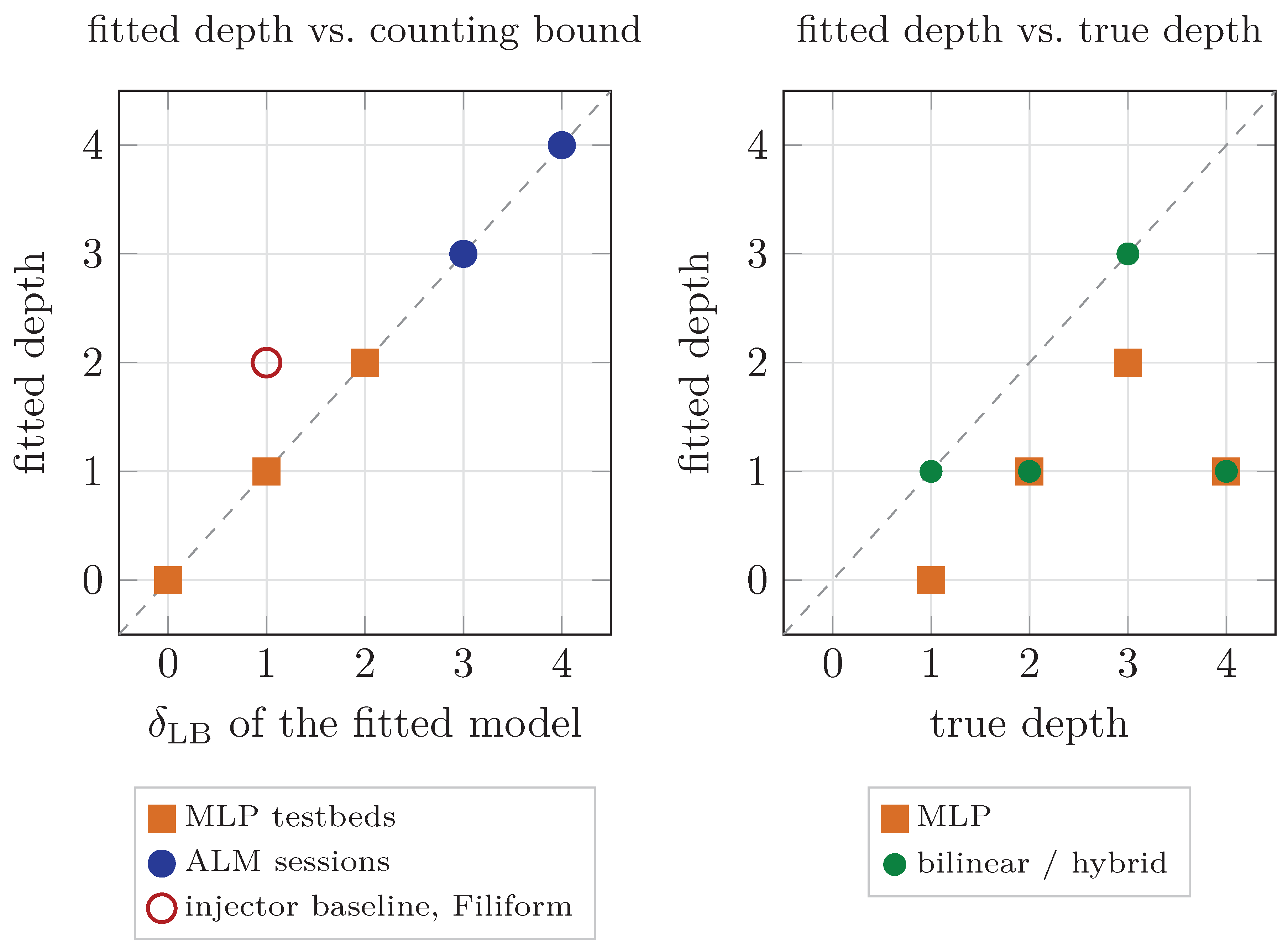
Reading. [measured] On the four testbeds reported, the MLP’s fitted depth equals the ${\delta }_{\mathrm{LB}}$ of the fitted model and is below the true depth in every case where the true depth exceeds ${\delta }_{\mathrm{LB}}$. The fitted models have $m=2$ inputs plus drift ($r=3$) here (Appendix B); results are for $\sigma =0$, $N={10}^4$. A perturbation study on KalmanChain $d=6$ (single input, $r=2$) shows depth 4 at $\eta =0$ dropping to 3 for $\eta \ge {10}^{-2}$, which is ${\delta }_{\mathrm{LB}}(6,2)$: small noise moves the estimate from the truth to the generic value.

9.3. Hybrid Bilinear-Plus-Residual Models

The hybrid model is $f_i\left(x\right)=A_{i}x+b_i+g_i\left(x\right)$ with $g_i$ an MLP initialised at zero. On affine testbeds the residual stays at zero and the model reduces to the bilinear one.

Table 7. Hybrid model, $\sigma =0$. “Cond.” is the condition number of the bracket stack at the estimated depth.

Testbed	True	Est.	Match	Cond.
Heisenberg(3)	1	1	✓	1.5
Bilinear(8,$r=2$)	3	3	✓	72
Engel(4)	2	1	×	135
Filiform(6)	4	1	×	$2.05\times {10}^5$

Table 7. Hybrid model, $\sigma =0$. “Cond.” is the condition number of the bracket stack at the estimated depth.

Testbed	True	Est.	Match	Cond.
Heisenberg(3)	1	1	✓	1.5
Bilinear(8,$r=2$)	3	3	✓	72
Engel(4)	2	1	×	135
Filiform(6)	4	1	×	$2.05\times {10}^5$

Reading. [measured] The hybrid recovers depth on the two affine testbeds and fails on the other two. The condition number explains at least the Filiform failure: its depth-4 signal sits five orders of magnitude below the level-0 signal and is effectively invisible in double precision. Amplifying the nonlinear terms by $100\times$ did not change the estimates, so this failure is structural rather than a matter of scale.

9.4. Matched-Spectrum Nulls

Table 8. Fitted depth versus matched null ($\sigma =0$).

Testbed	Fitted depth	Matched null
Heisenberg	1	0
Engel	1	1
Filiform	1	1
Bilinear	3	2

Table 8. Fitted depth versus matched null ($\sigma =0$).

Testbed	Fitted depth	Matched null
Heisenberg	1	0
Engel	1	1
Filiform	1	1
Bilinear	3	2

Reading. [measured] Where a fit genuinely recovers structure (Heisenberg, Bilinear) it exceeds the null; where it does not (Engel, Filiform) it equals the null. This is the calibration we want: the null tells us what “no structure” looks like for the estimator, and the fits that recover structure beat it. The P4 gate in §11.1 uses the same logic.

The P3 gate. [not met] The pre-registered gate required $90\%$ of testbeds recovered at $\sigma =0$; we obtained $2/4=50\%$. We read the failure as information: with the model classes we have, the estimator returns generic depth whenever the class cannot express the structure.

Figure 3. The learner speaks for itself. Left: fitted depth against the counting bound of the fitted model; overlapping points are drawn on top of each other (three ALM sessions at $(4,4)$; Engel and Filiform MLP fits at $(1,1)$). The open circle marks the injector-harness baseline for Filiform, which does not lie on the diagonal (see §12.2). Right: fitted depth against true depth for the four testbeds; the bilinear and hybrid fits are identical on these testbeds.

Figure 3. The learner speaks for itself. Left: fitted depth against the counting bound of the fitted model; overlapping points are drawn on top of each other (three ALM sessions at $(4,4)$; Engel and Filiform MLP fits at $(1,1)$). The open circle marks the injector-harness baseline for Filiform, which does not lie on the diagonal (see §12.2). Right: fitted depth against true depth for the four testbeds; the bilinear and hybrid fits are identical on these testbeds.

10. Act IV, Continued — Additive-Input Rate Networks (P3b)

The hypothesis. For a rate network $\dot{x}=-x+W{\varphi }_{\beta }\left(x\right)+Bu$ with additive input and increasing nonlinearity $\beta$, we expected depth to interpolate between the Krylov value $\lceil d/m\rceil -1$ and ${\delta }_{\mathrm{LB}}$. We tested $d=20$, $m=2$ with spectral radius $1.05$.

Table 9. Rate-network quantities ($d=20$, $m=2$). The “Krylov” column is the Krylov index of $J\left(p\right)$ with respect to B; it is not the Lie depth.

Variant	$\mathit{\beta }$	Krylov index	Estimator	Notes
Dense, additive	0.00	9	—	matches $\lceil 20/2\rceil -1$
Dense, additive	0.75	10	—
Dense, additive	1.00	$>15$	$\ge 9$	estimator non-convergent
Dense, state-dep	1.00	—	3	$={\delta }_{\mathrm{LB}}(20,3)$
Sparse, additive	1.00	$>12$	$\ge 9$	estimator non-convergent

Table 9. Rate-network quantities ($d=20$, $m=2$). The “Krylov” column is the Krylov index of $J\left(p\right)$ with respect to B; it is not the Lie depth.

Variant	$\mathit{\beta }$	Krylov index	Estimator	Notes
Dense, additive	0.00	9	—	matches $\lceil 20/2\rceil -1$
Dense, additive	0.75	10	—
Dense, additive	1.00	$>15$	$\ge 9$	estimator non-convergent
Dense, state-dep	1.00	—	3	$={\delta }_{\mathrm{LB}}(20,3)$
Sparse, additive	1.00	$>12$	$\ge 9$	estimator non-convergent

Interpretation. The table cannot be read as a measurement of Lie depth, for three reasons.

• The “Krylov” column is the Krylov index of the Jacobian, a property of $J\left(p\right)$. For generic J it equals $\lceil d/m\rceil -1=9$. Values 10 and $>15$ indicate that $J\left(p\right)$ is Krylov-deficient or numerically ill-conditioned at the reference points (for example, saturating tanh drives J toward $-I$, for which the Krylov span collapses to $\mathrm{span}B$). That is a statement about conditioning, not about Lie depth. We did not check whether the reference points are equilibria, which is the case in which Prop. 3(c) applies.
• For nonlinear drift the Krylov index is only an upper bound on depth (Prop. 3(c)), and Hessian brackets (Prop. 3(a)) contribute directions it ignores.
• The estimator column for the additive nonlinear variants is “$\ge 9$, non-convergent” at $d=20$, and the finite-difference estimator degrades at $d>16$ for nonlinear systems (Appendix C).

Status. [inconclusive] The measured $3={\delta }_{\mathrm{LB}}(20,3)$ for the state-dependent variant agrees with the counting bound; whether additive nonlinear drift also reaches it, as the Hessian brackets suggest it might, was not tested because the estimator did not converge. A rerun with exact automatic-differentiation brackets would settle it. We therefore make no claim that state-dependence is the mechanism that reduces depth to ${\delta }_{\mathrm{LB}}$; that question remains open.

11. Act IV, Continued — Real Data and World Models

11.1. P4: CRCNS ALM-4 Photostimulation Sessions

Method. Four sessions from CRCNS alm-4, each with 19–23 single units and 47–63 photostimulation trials. The input $u\left(t\right)$ is extracted from aom_input_trace at $10\mathrm{kHz}$ and binned to $100\mathrm{ms}$; spike counts are smoothed with a $150\mathrm{ms}$ Gaussian; PCA at $95\%$ variance gives $d_{\mathrm{eff}}\in \{6,12,13,14\}$. A hybrid bilinear plus zero-init MLP is fitted per session, with 200 reference points, 50 matched-spectrum nulls and 500 bootstrap resamples over sessions. Input dimension is one photostimulus channel, so $r=2$.

Result. [inconclusive] Every session’s fitted depth equals its ${\delta }_{\mathrm{LB}}$. The pre-registered gate, that the fitted profile must beat the null at $95\%$ confidence, is not met: the fitted CI $[3,4]$ overlaps the null $p_{95}=4$. We want to be exact about what this does and does not say. It is consistent with Corollary 1. It is equally consistent with the estimator being unable to see any structure in nineteen to twenty-three units and fifty-odd trials; the matched null reaches the same value. We therefore do not read it as “confirming the generic-bound prediction on real neural recordings”; we read it as a result that cannot distinguish the generic bound from a lack of power.

Table 10. Real ALM sessions.

Session	${\mathit{d}}_{\mathbf{orig}}$	${\mathit{d}}_{\mathbf{eff}}$	Fitted depth	${\mathit{\delta }}_{\mathbf{LB}}$	Null ${\mathit{p}}_{95}$
ANM314746_20151020	23	13	4	4	4
ANM314746_20151021	19	6	3	3	3
ANM314746_20151022	21	14	4	4	4
ANM314756_20151020	20	12	4	4	4

Table 10. Real ALM sessions.

Session	${\mathit{d}}_{\mathbf{orig}}$	${\mathit{d}}_{\mathbf{eff}}$	Fitted depth	${\mathit{\delta }}_{\mathbf{LB}}$	Null ${\mathit{p}}_{95}$
ANM314746_20151020	23	13	4	4	4
ANM314746_20151021	19	6	3	3	3
ANM314746_20151022	21	14	4	4	4
ANM314756_20151020	20	12	4	4	4

11.2. P5: H-JEPA Checkpoints

Method. Nine H-JEPA [9] Cube checkpoints (three hierarchy levels by three seeds). The level-0 predictor $F(z,a)$ is evaluated with the action broadcast $5\times$ to match the action_embed input width ($5\times 5=25$), then passed through action_embed and predictor. The effective dimension is the PCA dimension at $95\%$ variance of $\{F(z,a_0)-z\}$ over 100 random z.

Result. [measured] $d_{\mathrm{eff}}=75\pm 0.3$ across the nine checkpoints ($74,75,75,75,75,75,74,75,75$), apparently insensitive to hierarchy level and seed. ${\delta }_{\mathrm{LB}}(75,6)=2$. A full depth measurement was not made: at $d_{\mathrm{eff}}>21$ depth-2 brackets cost about $216\times$ depth-1 and exceeded the budget. The statement “fitted depth is predicted to equal 2” is a prediction, not a result.

12. Act V — Bribing the Witness: Trying to Fix the Learner (Bracket-Injector)

The bracket-injector adds to the reconstruction loss a term that rewards full rank of the depth-k bracket stack and penalises full rank at shallower depths.

12.1. The loss

Let $f_0,\dots ,f_m$ be the fitted fields, k the target depth, $x^{\left(1\right)},\dots ,x^{\left(N_b\right)}$ reference points, and $B_j\left(x\right)\in {\mathbb{R}}^{n_j\times d}$ the stack of brackets of depth $\le j$ at x.

$$\begin{array}{cc}\hfill {\mathcal{L}}_{\mathrm{span}}& =-{\displaystyle \frac{1}{d_{\mathrm{eff}}}}{\displaystyle \sum _{i=1}^{d_{\mathrm{eff}}}}\log \left({\sigma }_i{\left(B_k\right)}^2+ϵ\right),\hfill \end{array}$$

(5)

$$\begin{array}{cc}\hfill {\mathcal{L}}_{\mathrm{supp}}& ={\displaystyle \sum _{j=0}^{k-1}}{\beta }_j\max {\left(0,{\sigma }_{d_{\mathrm{eff}}}\left(B_j\right)-\tau \right)}^2,\hfill \end{array}$$

(6)

$$\begin{array}{cc}\hfill \mathcal{L}& ={\mathcal{L}}_{\mathrm{rec}}+\lambda \left(t\right)\left({\mathcal{L}}_{\mathrm{span}}+{\mathcal{L}}_{\mathrm{supp}}+{\mathcal{L}}_{\mathrm{reg}}\right),\hfill \end{array}$$

(7)

where ${\mathcal{L}}_{\mathrm{reg}}$ is a regulariser on the fields with weight ${\lambda }_{\mathrm{reg}}$. The weight $\lambda \left(t\right)$ is annealed from 0 to ${\lambda }_{\max }$ over 1000 steps after a 500-step warm-up, with $\tau ={10}^{-3}$, $ϵ={10}^{-6}$, ${\beta }_j=1$, ${\lambda }_{\mathrm{reg}}={10}^{-3}$, $N_b=30$.

12.2. Gates 1 and 2: The Machinery Is Sound

Gate 1 (gradient). [measured] In float64, on a properly posed case ($d=5$, $m=2$, $d_{\mathrm{eff}}=4$, $k=1$; base rank $3<4$ so suppression is inactive), the maximum relative error of $\partial {\mathcal{L}}_{\mathrm{span}}/\partial \theta$ against finite differences was $9.5\times {10}^{-7}$. A diagnostic bracket-norm loss without an SVD gave $9.2\times {10}^{-6}$, isolating numerical error to svdvals and motivating svd().S in the loss. Gate 1: passed.

Gate 2 (baseline). [measured] With ${\lambda }_{\max }=0$, the PyTorch implementation is compared with the numpy pipeline used in §9: Heisenberg 0, Engel 1, Filiform 2, Bilinear 2, none of which matches the true depth ($0/4$, as intended for a no-prior baseline). Gate 2: passed, with one discrepancy: the Filiform baseline here is 2, one level above the value in Table 6. We report both unadjusted.

12.3. Gate 3: Injector on Four Testbeds

Sweeps were ${\lambda }_{\max }\in \{0.01,0.03,0.1\}$ (Heisenberg, Bilinear) and $\{0.03,0.1\}$ (Engel, Filiform), $\sigma =0$, $N={10}^4$.

Table 11. Bracket-injector: estimated versus target depth.

Testbed	True k	${\mathit{\delta }}_{\mathbf{LB}}$	Baseline	Injector	Outcome
Heisenberg(3)	1	0	0	1	pass (degenerate)
Engel(4)	2	1	1	1	fail
Filiform(6)	4	1	2	2	fail
Bilinear(8,$r=2$)	3	2	2	2	fail

Table 11. Bracket-injector: estimated versus target depth.

Testbed	True k	${\mathit{\delta }}_{\mathbf{LB}}$	Baseline	Injector	Outcome
Heisenberg(3)	1	0	0	1	pass (degenerate)
Engel(4)	2	1	1	1	fail
Filiform(6)	4	1	2	2	fail
Bilinear(8,$r=2$)	3	2	2	2	fail

Heisenberg $d=3$. With $m=2$ the base fields already span rank 3; the target is reached by suppressing depth-0 rank from 3 to 2, which is trivially available. This does not show the injector overcoming the generic bias.

Engel $d=4$. [not met] The prior loss falls from 423 to $-4.37$, but the estimator reads singular values around $2\times {10}^{-4}$ against its threshold $\tau ={10}^{-3}$. One possibility is that training is simply too short or the threshold too strict. A second is visible in the loss itself: ${\mathcal{L}}_{\mathrm{span}}$ averages $\log {\sigma }_i^2$ over the $d_{\mathrm{eff}}$ singular values, so it can be negative, i.e. satisfied on average, while the smallest singular value is tiny, because a few large values compensate. The estimator thresholds the smallest one. That is a mismatch between the training objective and the decision rule, and it would persist at longer training.

Filiform $d=6$. [not met] ${\mathcal{L}}_{\mathrm{prior}}$ reached $2.28\times {10}^{14}$ at step 600 and $1.24\times {10}^{13}$ at step 1800. One natural reading is that suppression and span terms conflict until SGD drives all brackets to zero. The loss definition does not support that: with $ϵ={10}^{-6}$ each $-\log ({\sigma }^2+ϵ)\le \log (1/ϵ)\approx 13.8$, so ${\mathcal{L}}_{\mathrm{span}}\le 13.8$ no matter how small the singular values become, and float64 cannot represent singular values near $e^{-{10}^{13}}$ in any case. A value of order ${10}^{14}$ must therefore come from ${\mathcal{L}}_{\mathrm{supp}}$ (or ${\mathcal{L}}_{\mathrm{reg}}$), i.e. large shallow-depth singular values. The more plausible mechanism is scale blow-up: $-\log {\sigma }^2$ is unbounded below as $\sigma \to \infty$, so SGD can inflate field magnitudes to satisfy the span term (depth-4 brackets scale as the fifth power of the field norm), and the squared suppression penalty then explodes.

Bilinear $d=8$, $r=2$. [not met] The fitted model has $m=2$ inputs and a drift, so $r=3$ and ${\delta }_{\mathrm{LB}}(8,3)=2<3$: the generic solution reaches rank 8 at depth 2 and the target depth 3 requires suppressing that rank, i.e. producing non-generic fields. We have no proof that a gradient-level regulariser cannot do this; we observed only that this one did not, with the suppression term active.

12.4. What the Failure Does and Does Not Show

Gate 3: failed ($1/4$, degenerate). We identify three failure modes; each is an analysis from the loss definition and none was confirmed by a separate experiment:

(a)

Engel: objective/decision mismatch (mean-log span term versus smallest-singular-value threshold). [heuristic]

(b)

Filiform: instability from an unbounded barrier and absent scale control, rather than vanishing singular values. [heuristic]

(c)

Bilinear: the target requires non-generic structure; whether this is out of reach for gradient-level priors in principle or merely for this loss is [open].

Implications. [not met] The injector as designed does not move learners off the generic bound. Three variants are suggested directly by the diagnoses and were not run: (i) replace the mean-log span by a bounded barrier on ${\sigma }_{d_{\mathrm{eff}}}$ itself (a smooth hinge, or $-\tanh \left(\alpha \sigma \right)$) with $\tau$ tied to the estimator’s threshold; (ii) normalise fields (or brackets) to remove the scale degeneracy; (iii) replace the MLP by a parametrisation whose class contains the target depth (polynomial or bilinear basis), which is the setting in which §9 showed exact recovery.

13. Epilogue — Discussion

13.1. Summary

The algebra is clean: depth is at least ${\delta }_{\mathrm{LB}}$, can equal it, and a random system does equal it. The physics on designed systems agrees with the algebra. The surprise, such as it is, is on the learning side. A fitted control-affine model has a depth that the model class and $d_{\mathrm{eff}}$ largely determine; where the class can represent the system’s special structure (affine testbeds) the structure is recovered, and where it cannot, the fit reports the generic value instead. In parking terms: an observer can only count the manoeuvres its vocabulary allows. The bracket-injector was an attempt to turn that observation into a method and it did not work as designed.

13.2. Threats to Validity

• Small n. Four testbeds in P3, four sessions in P4.
• Estimator and model are entangled. “Fitted depth” mixes the model class, the rank threshold and the reference points; nulls partly separate these.
• $d_{\mathrm{eff}}$ is thresholded. PCA at $95\%$ variance; P5’s value may be sample-limited.
• Estimator range. The finite-difference JVP estimator is reliable only for $d\le 16$ on nonlinear systems, which affects P3b.
• Protocol-dependent constants. The noise slope c depends on segment duration and on whether t is pinned or maximised.

13.3. Claim Ledger

Table 12. All claims and their status.

Claim	Section	Status	Evidence
Counting lower bound $\delta \ge {\delta }_{\mathrm{LB}}$	§3	classical	Thm. 1
Tightness on nilpotent groups	§3	classical	Thm. 2
No universal upper bound	§3	proved	Prop. 1
Generic attainment (polynomial class)	§4	proved	Thm. 3
Learned models as generic draws	§4	heuristic	Cor. 1; Conj. 1 open
Additive-input bracket structure	§4	proved	Prop. 3
State-dependent input $\to {\delta }_{\mathrm{LB}}$	§4	conditional	Prop. 4; witness missing
Accessibility, one-sided inputs	§7	measured	15/16; one tolerance-unstable
${\sigma }_{\min }\propto T^{k+1}$	§7	measured	7 exact fits; 3 looser
Open-loop log law	§8	measured	$R^2\ge 0.95$ in all rows
c depends on t, predicted by (4)	§5,§8	heuristic + measured	0.38 vs 0.397; 0.51 vs 0.462
Amplitude ≡ timing, driftless	§8	sanity check	flow depends on product
Closed-loop ceiling $+1$ to $+3$	§8	measured	Table 4
Bilinear fit recovers affine truth	§9	measured	2/2 affine testbeds
MLP fit sits at ${\delta }_{\mathrm{LB}}$	§9	measured	4 testbeds, $\sigma =0$
P3 gate (90% at $\sigma =0$)	§9	failed	2/4
P3b additive hypothesis	§10	inconclusive	Krylov index ≠ Lie depth
ALM sessions	§11	inconclusive	fitted $={\delta }_{\mathrm{LB}}=$ null
H-JEPA $d_{\mathrm{eff}}$	§11.2	measured	$75\pm 0.3$; depth not measured
Injector Gates 1, 2	§12	measured	rel. err. $9.5\times {10}^{-7}$; baseline 0/4
Injector Gate 3	§12	failed	1/4 (degenerate)
Injector diagnoses (a), (b)	§12	heuristic	from loss definition, untested

Table 12. All claims and their status.

Claim	Section	Status	Evidence
Counting lower bound $\delta \ge {\delta }_{\mathrm{LB}}$	§3	classical	Thm. 1
Tightness on nilpotent groups	§3	classical	Thm. 2
No universal upper bound	§3	proved	Prop. 1
Generic attainment (polynomial class)	§4	proved	Thm. 3
Learned models as generic draws	§4	heuristic	Cor. 1; Conj. 1 open
Additive-input bracket structure	§4	proved	Prop. 3
State-dependent input $\to {\delta }_{\mathrm{LB}}$	§4	conditional	Prop. 4; witness missing
Accessibility, one-sided inputs	§7	measured	15/16; one tolerance-unstable
${\sigma }_{\min }\propto T^{k+1}$	§7	measured	7 exact fits; 3 looser
Open-loop log law	§8	measured	$R^2\ge 0.95$ in all rows
c depends on t, predicted by (4)	§5,§8	heuristic + measured	0.38 vs 0.397; 0.51 vs 0.462
Amplitude ≡ timing, driftless	§8	sanity check	flow depends on product
Closed-loop ceiling $+1$ to $+3$	§8	measured	Table 4
Bilinear fit recovers affine truth	§9	measured	2/2 affine testbeds
MLP fit sits at ${\delta }_{\mathrm{LB}}$	§9	measured	4 testbeds, $\sigma =0$
P3 gate (90% at $\sigma =0$)	§9	failed	2/4
P3b additive hypothesis	§10	inconclusive	Krylov index ≠ Lie depth
ALM sessions	§11	inconclusive	fitted $={\delta }_{\mathrm{LB}}=$ null
H-JEPA $d_{\mathrm{eff}}$	§11.2	measured	$75\pm 0.3$; depth not measured
Injector Gates 1, 2	§12	measured	rel. err. $9.5\times {10}^{-7}$; baseline 0/4
Injector Gate 3	§12	failed	1/4 (degenerate)
Injector diagnoses (a), (b)	§12	heuristic	from loss definition, untested

13.4. Open Problems

• Prove Conjecture 1, or find the class where it fails.
• Exhibit a witness for Proposition 4, and settle whether additive nonlinear drift reaches ${\delta }_{\mathrm{LB}}$ (exact AD brackets at $d=20$).
• Make an estimator whose failure mode is “abstain” rather than “return the generic value”: calibrate against nulls and report when it cannot separate from them.
• Run the three injector variants of §12.
• Measure H-JEPA depth at $d_{\mathrm{eff}}\approx 75$ with larger sample size and exact brackets.
• Quantitative bounds under one-sided inputs.
• Prove the form (4) for $c\left(t\right)$, or replace it.

Appendix A.1. Proof of Proposition 2 (Time Cost)

Write $P_k\left(t\right)$ for the protocol of depth k, a product of $n_k$ flows of duration t. For $k=0$, $P_0=e^{t{f}_i}$, so $n_0=1$ and $P_0=\exp \left(t{f}_i\right)$. Suppose $P_{k-1}=\exp \left(t^k{B}_{k-1}+O\left(t^{k+1}\right)\right)$ with $B_{k-1}$ of depth $k-1$. Define $P_k=e^{t{f}_i}{P}_{k-1}{e}^{-t{f}_i}{P}_{k-1}^{-1}$ (reversed flows require signed inputs). Baker–Campbell–Hausdorff gives

$$e^X{e}^Y{e}^{-X}{e}^{-Y}=\exp \left([X,Y]+\frac{1}{2}[X,[X,Y]]+\frac{1}{2}[Y,[X,Y]]+\dots \right),$$

here with $X=t{f}_i$ and $Y=t^k{B}_{k-1}+O\left(t^{k+1}\right)$, so $P_k=\exp \left(t^{k+1}[f_i,B_{k-1}]+O\left(t^{k+2}\right)\right)$, a bracket of depth k. The segment count satisfies $n_k=2n_{k-1}+2$, $n_0=1$, whose solution is $n_k=3·2^k-2$.

Appendix A.2. Proof of Proposition 3

(a) With $[f,g]=Dgf-Dfg$, for constant $b_k$: $[f_0,b_k]=D{b}_k{f}_0-D{f}_0{b}_k=-J{b}_k$. Then $[b_i,-J{b}_k]=D(-J{b}_k)b_i-D{b}_i(·)=-\left({\partial }_{b_i}J\right)b_k=-{\partial }^2{f}_0(b_i,b_k)$. For constant $b_i,b_k$, $[b_i,b_k]=0$.

(b) Let $g_0=b_k$ and $g_{j+1}=[f_0,g_j]=D{g}_j{f}_0-J{g}_j$. If $f_0\left(p\right)=0$ then $g_{j+1}\left(p\right)=-J\left(p\right)g_j\left(p\right)$, so $g_j\left(p\right)={(-J\left(p\right))}^j{b}_k$. If $f_0$ is affine, J is constant and every $g_j={(-J)}^j{b}_k$ is constant, so $D{g}_j=0$ and the same recursion holds at every p.

(c) Containment follows from (b): the values $g_k^{\left(j\right)}\left(p\right)$ for $j\le \delta$ are depth-$\le \delta$ brackets. Hence $\dim {\mathfrak{L}}_{\delta }\left(p\right)\ge \dim \mathrm{span}{\left\{J^j{b}_k\right\}}_{j\le \delta }$, and full rank of the Krylov span at $\delta =k_K$ implies ${\mathrm{depth}}_p\le k_K$. For affine $f_0$ with constant $b_i$, every left-nested bracket containing some $b_i$ and another constant field vanishes, and $[f_0,c]=-Jc$ for constant c, so the nonzero brackets are $f_0$ and ${\mathrm{ad}}_{f_0}^j{b}_k$, giving the equality.

Appendix A.3. Direction of the Krylov Bound

Containment of the Krylov directions in ${\mathfrak{L}}_{\delta }$ shows the Lie span is at least as large as the Krylov span, so the depth needed is at most the Krylov index. A lower bound on depth would need an upper bound on $\dim {\mathfrak{L}}_{\delta }$, which holds for affine $f_0$ (equality in (c)) but not for nonlinear $f_0$, where (a) provides further directions.

References

1. W.-L. Chow. Über Systeme von linearen partiellen Differentialgleichungen erster Ordnung. Math. Ann. 117:98–105, 1939.
2. P. K. Rashevskii. Connecting two points of a completely nonholonomic space by an admissible curve. Uch. Zap. Ped. Inst. im. Liebknecht 2:83–94, 1938.
3. H. J. Sussmann and V. Jurdjevic. Controllability of nonlinear systems. J. Differential Equations 12:95–116, 1972.
4. E. Witt. Die Unterringe der freien Lieschen Ringe. Math. Z. 64:195–216, 1956. [CrossRef]
5. C. Reutenauer. Free Lie Algebras. Clarendon Press, 1993.
6. A. Nagel, E. M. Stein and S. Wainger. Balls and metrics defined by vector fields I. Acta Math. 155:103–147, 1985. [CrossRef]
7. M. Gromov. Carnot–Carathéodory spaces seen from within. In Sub-Riemannian Geometry, Birkhäuser, 1996.
8. A. Agrachev, D. Barilari and U. Boscain. A Comprehensive Introduction to Sub-Riemannian Geometry. Cambridge University Press, 2020.
9. Zhang, Terver, Rabbat, LeCun and Balestriero. H-JEPA. arXiv:2610.06805, 2026.
10. M. Mostafa. depthwidth: code accompanying this paper. MIT licence. https://github.com/liebracketdepthwidth-eng/How-Deep-Is-the-Control-, 2026.