

Submitted:
29 October 2026
Posted:
30 October 2026
You are already at the latest version
Abstract
Inspection of markings on integrated circuit (IC) packages requires a large dataset of images of defective markings. Such images are scarce and seldom shared publicly. This paper introduces a set of physics-informed guidelines for generating synthetic images of defective IC markings from images of defect-free markings. These guidelines build each defect type from its physical cause, distinguish defects of the marking from defects of the package surface, and produce defect labels. Four common defect types of scratch, contamination, missing text and smeared text are implemented, together with images that combine two or three defect types. In addition, the steps for adding further defect types are provided. The guidelines are then evaluated on a small dataset of real images of marking defects. It is shown that the generated images are close to the real images of defective markings in terms of four quantitative similarity measures. It is also shown that a detector trained on the generated images alone detects most of the real defects. In essence, this paper provides a dataset of 6,000 synthetic IC marking images for six image classes, named ICMarkingSynthetic, to enable IC marking inspection studies, as well as the guidelines for generating these and other defect types.
Keywords:
openly licensed dataset of synthetic images of IC marking defects
; inspection of integrated circuit markings
; generating synthetic images of IC marking defects
; physics-informed guidelines for image generation
; automated optical inspection of IC markings
1. Introduction
Laser-etched or ink-printed markings are placed on the package or cover of Integrated Circuits (ICs) to identify the part number or chip id, the manufacturer logo, the date of manufacture and the pin-1 indicator. Inspection of these markings is carried out during the manufacturing process to avoid sending ICs with defective markings, such as incompletely printed or obscured characters, to customers. Automated Optical Inspection (AOI) systems are used to perform this inspection task [1]. Early systems inspected markings with hand-designed features and rules [2,3,4]. More recent systems use deep learning models such as the ones discussed in [5,6]. A deep learning-based inspection model can be adapted to each IC by re-training rather than by re-engineering hand-designed rules.
A problem encountered on an actual IC production line is that images of defective markings are scarce, as the production line is designed for defects not to occur. In other words, an actual production line yields mostly defect-free IC markings and only very few defective markings. Another problem is that such images labeled by an expert are often proprietary and not publicly available. Inspection systems reported in the literature include a study reporting 11 images of missing characters among 2,043 images [7], and another study reporting 58 images of a single package, 25 of them defective [1]. Unfortunately, no comprehensive procedure exists in the literature for generating images of defective IC markings when real defective images are not available.
Generating synthetic images is a way to set up an inspection system before real defective images become available. Existing synthetic image generation methods suffer from the following shortcomings. Generic synthetic image generation approaches paste patches or noise textures onto defect-free images, e.g. [8,9,10]. However, they do not model a scratch, a deposit or a missing character, and a detector trained on such images is not shown what these defects look like. Copy-based image generation methods in the earlier IC marking studies paste real defective patches onto defect-free images. They need real images of defective markings and can only recombine those defects that are already observed. Generative models trained on defect examples, e.g. [11,12], produce a diverse set of images. However, they need real images of defective markings for training, which are scarce [13]. Generative models driven by text prompts need no defect example, e.g. [14], but their output is not tied to a stated physical cause. For example, as reported in [1], the enhanced CycleGAN approach in [15] failed to produce realistic defective images from a few available images. Geometry-based synthetic image generation methods build defective images from geometric distortions without using any real images of defective markings [16,17,18,19]. They do not address how the generated images are checked against a few real defective images that may exist.
This paper introduces a set of physics-informed guidelines to generate synthetic images while overcoming the above shortcomings. Defect types incorporate damage to the package surface, foreign material deposited on it, or an error in the marking process [1,2,20]. A region model is used to separate a marking from its package area so that each defect can be rendered where it occurs. Every defect is rendered onto a known defect-free image, so its label is exact. A calibration step compares shape and intensity measurements of the generated defects with those of a few real images of defects under a stated pass rule. In this way, the appearance is checked by measurement rather than by visual inspection. These guidelines are demonstrated for four defect types and combinations, scratch and contamination on the surface as well as missing and smeared text. It is also explained how further defect types of interest can be added to this synthetic image generation framework. Figure 1 illustrates the guidelines and displays some generated image examples.
Because the openly licensed images used in this work contain no real defects, the guidelines are applied to the dataset in [1], which has some real images of defective markings. Three aspects are examined: how the generated images of defects resemble real ones in terms of four distribution distances, how the generated images of defects compare with the rule-based inspection approach in that earlier study, and how a detector trained on synthetic images responds to real images of defects.
The contributions in this paper include the following. A set of physics-informed guidelines for generating synthetic images of defective IC markings. An evaluation of the guidelines using the dataset in [1] from three perspectives: realism against real images of defects and three other synthetic image generation methods, recognition by the rule-based inspection method in [1], and transfer of detectors trained on synthetic images to real images. The most notable contribution of this paper is the introduction of a dataset of 6,000 synthetic images of IC markings, named ICMarkingSynthetic. This dataset is generated by the introduced guidelines using 40 openly licensed images, and it comes with labels, boxes, polygons, exact masks, severity levels and per-image provenance. The dataset and the generator that produced it are both made publicly available.
2. Background and Prior Approaches
2.1. Marking Inspection and Its Data Requirement
A marking inspection system examines whether the characters on an IC package are present, complete and legible, for every IC that passes a production line. Rule-based inspection systems detect missing ink, smear, broken characters and misprint by projection, correlation and morphological operations against a reference marking [2], segment and classify characters [3], or compare feature-extraction techniques [4]. These rule-based systems are adapted to a new IC marking by considering new references and thresholds. Learned inspection systems, such as the weakly supervised detector in [5] and the compact ICMarkingNet in [6], are adapted by re-training. The above learned inspection systems are trained on images which are not publicly available. The IC text dataset ICText, available on request, annotates character quality attributes (low contrast, blurry, broken) of 100,152 characters rather than defect classes and masks [21]. One way to avoid images of defects altogether is to learn from defect-free images and flag reconstruction residuals [22,23]. For a new defect type, a learned marking inspection system needs to start from very few example images of defects.
In an earlier study in [1], 58 real images consisting of 33 defect-free images and 25 images of defects were considered over five defect classes. A rule-based inspection system whose thresholds were learned by a bandit procedure was then used. The training data was enlarged by blending defect patches cut from the real images onto defect-free images. In a later study in [24], the auto-labeling method was extended to include two additional defect types. The real images of the above studies are the only real test material available for IC markings. They are used here as the evaluation instrument.
2.2. Approaches to Synthetic Defect Generation
The previous approaches differ in what they require as input and what they produce in return. The surveys in [25] and [26] use similar groupings. Table 1 compares the four groups by the properties that matter for marking inspection, and the evidence behind each row is stated in what follows.
Generic anomaly synthetic image generation needs only normal images. CutPaste pastes patches of an image onto itself [8], DRAEM fills Perlin-noise masks with external textures [9], NSA blends patches from other images by Poisson editing [10], and GLASS synthesizes anomalies at the feature and image level [27]. In [13], it was shown that such an approach can be used to train anomaly detectors effectively even though its images are not realistic. Such an approach trains a detector of departures from normal, not a detector of what a scratch or a missing character looks like. Copy-based synthetic methods reuse real defect pixels, as the patch-blending method of the IC marking study in [1]. Their defects are real in appearance, but they cannot produce a defect type for which no real example image exists. Generative models produce new samples rather than copies. Defect-GAN and SDGAN use adversarial training [11,33], DFMGAN manipulates StyleGAN2 features with a few defect images [28], AnomalyDiffusion and DualAnoDiff adapt latent diffusion models [29,34], and RealNet synthesizes anomalies with a diffusion model [35]. Stable Diffusion was conditioned on defect geometry with as few as 120 annotated images in [12], DefectFill fine-tunes an inpainting model on a few reference defects [30], and the most recent systems use model-agnostic realistic anomaly generation [14] or an agent that composes synthesis tools [36]. In [37], defective epoxy-drop images for die attachment were generated by a CycleGAN model trained under an enhanced loss function, which again required real image examples of defects. Even the few-shot variants need image examples per class [28,30], and training a generative model is computationally expensive [13]. Furthermore, a generative model reproduces a learned distribution rather than a physical cause, so whether its output matches defects that occur in production needs to be checked separately. To see how a generative model behaves when no defect example is given, this paper applies a general-purpose latent diffusion model, Stable Diffusion Inpainting [38], to the reference images with text prompts.
Procedural and physics-based synthetic image generation builds each defect from a geometric and a material model and needs no image of defects. In [16], scratches and dents were parametrized for virtual inspection. In [31,39], machined-metal textures were modeled procedurally, and in [31] the similarity of synthetic and real images was measured. ScratchSim rendered Bezier-curve scratches as normal-map perturbations [19], and scratches and dents were generated by procedural bump mapping in [32]. In [17], a physical cross-section was mapped to each scratch pixel and the segmentation IoU was raised from 0.66 to 0.83 with 20 real images. In [18], physics-inspired bumps, dents and scratches were applied to automotive surfaces. In the semiconductor domain, SCRS sampled chip-scratch masks from fitted statistics and filled them with a diffusion model [40], and synthetic ink and crack defects were generated for an in-house chip dataset in [41]. These studies show that model-based synthetic image generation can replace images of defects for surface damage, and the guidelines presented in this work follow the same principle. The previous approaches leave the following issue unaddressed. All of them model a defect as damage to a surface, whereas a marking defect is a change of the printed information. Where realism was measured, as in [31], it was measured for a texture as a whole. None of the prior approaches combines cause-derived construction, exact annotation and a stated calibration procedure against the few real images of defects of the same kind that may exist, which is the combination needed for IC marking defects.
Models of how a printed marking degrades exist outside the inspection literature. In [42], broken printed characters were modeled by distance-dependent pixel flipping and the model was validated against real degraded characters with a two-sample permutation test. DocCreator and Augraphy provided procedural ink degradations for document images in [43,44], and OmniPrint synthesized printed characters with stroke-width and elastic transforms [45]. These tools act on rendered or binary text, whereas an IC marking is a photographed glyph on a textured surface. As a result, the degradation needs to be applied to the marking above the body. The physical causes of marking defects are documented. On epoxy mold compound, line width and depth govern mark visibility and filler left in the laser line causes uneven reflection [46], and ablation efficiency depends on filler size [47]. In laser marking, missing marks have been traced to a contaminated laser head, excessive or insufficient depth to unstable laser power, blurred marks to fluctuations of the electrical supply, and misalignment to vibration of the platform [20]. Our defect models described in Section 3 are derived from these causes.
2.3. Evaluation of Synthetic Images of Defects
A synthetic defect needs to appear realistic and useful, and these two attributes are measured differently. Realism is measured by comparing the distributions of real and synthetic images in a feature space. The Fréchet Inception Distance [48,49] has a finite-sample bias that depends on the model evaluated [50], which matters when only a few images are available, as is the case here. The Kernel Inception Distance (KID) uses the squared maximum mean discrepancy with a cubic kernel and involves an unbiased estimator [51,52]. CMMD uses CLIP embeddings with a Gaussian-kernel MMD [53]. No single metric closely follows human judgment, and DINOv2 features [54] agree with it better than Inception features [55]. For this reason, this paper reports realism on more than one feature space and states the uncertainty due to the small number of real image samples.
Usefulness is measured by training a model on synthetic images and testing it on real ones. It cannot be inferred from realism, since ASBench found weak or no correlation between image metrics and downstream detection [56]. Domain randomization showed that detectors trained on non-photorealistic renderings transferred to real images [57,58], and realism was compared with randomization for industrial detection in [59]. Synthetic-only training reached a substantial part of real-only detection performance for scratches and surface defects, typically between one half and four fifths depending on the dataset, detector and metric [19,60], and a small share of real images, added by fine-tuning or mixed training, narrowed the remaining gap [19,61]. In ISP-AD, for example, ten real defects raised the Matthews correlation coefficient from 0.81 to 0.91 [62]. These findings define the two task-based tests in this paper, transfer of a synthetic-only detector and adaptation with a few real images. Both need real images. The publicly available industrial anomaly benchmarks contain no IC markings [63,64,65,66], the closest being the PCB dataset DsPCBSD+ [67]. The evaluation is therefore carried out on the real images of the IC marking study in [1]. Table 2 provides the dataset of this paper beside the public datasets closest to the task. None of the public datasets contains defects of a marking, the IC text dataset annotates character quality rather than defects, and the one with real IC marking defect set is small and not public. This is the gap that this paper fills.
3. Introduced Physics-Informed Guidelines
3.1. Overview and Design Requirements
The guidelines introduced in this paper provide a procedure for generating labeled images of defective IC markings from images of defect-free markings. They are designed to meet five requirements that follow from Section 2. No real defect image may be needed for generation. Each defect type must reproduce the appearance of that type rather than a generic irregularity. Defects of the marking must be covered as well as defects of the surface. Every label must be exact. The generated appearance must be checked against whatever real defects exist. The procedure is organized as six decisions, each answering one question (see Figure 1): what part of the image may be modified (the region model, Section 3.2), what the inspection camera produces (the capture model, Section 3.3), what physical process causes each defect (the defect models, Section 3.4), how severe the defect is and what labels are created (severity, Section 3.5), how the result is checked against real defects (calibration, Section 3.6), and how a further defect type can get added (further defects, Section 3.7). Where real examples exist, the calibrated output is evaluated on them before release; otherwise, indirect checks are reported (addressed in Section 5). The generator used in this paper provides one implementation of the guidelines. The four defect types implemented, scratch, contamination, missing text and smeared text, together with their combinations, serve as worked examples. The term physics-informed is used in the following sense. Each defect model is derived from the documented physical cause of the defect, and the appearance it produces is a chosen image-formation approximation whose free parameters are set from measurements of real defects. The models are not optical simulations. The terminology is fixed here. These four are the commonly encountered defect types. An image belongs to one of six image-level classes: defect-free, one class per single defect type, and combined, which holds two or more defects. Combined is therefore not a fifth defect type but an image-level class in which each defect keeps its own type, mask, polygon and box.
Two rules hold throughout. No real defect pixel enters the generation. Real images of defects are measured during calibration, and only the resulting descriptor statistics adjust the parameters. Every image is reproducible on its own. All random draws come from a generator seeded by a hash of the source image identifier, the capture index and the defect type, so a change to one defect type does not alter the images of another. The notation is as follows. I denotes a captured gray-scale image, F the mask of the molded face, T ⊂ F the mask of the marking and S ⊂ F the mask of fixed surface features such as the pin-1 dimple. I1 is a defect image and M ⊂ F is its exact mask. The severity is s ∈ {0.25,0.5,0.75,1.0} denoting the levels low, medium, high and severe, respectively. Gσ* indicates Gaussian filtering with standard deviation σ pixels and clip8 indicates clipping to the 8-bit range. The expressions and parameter values not needed to follow the approach are mentioned in Appendix A, and Table A1 lists all the symbols.
3.2. Region Model: What May Be Modified
A marking defect and a surface defect occur in different places, and the region model makes the distinction explicit (see Figure 2). For each source image, three masks are derived once and reviewed manually. The face mask F is the package body located by edge and threshold detectors and inset by a margin. The marking mask T holds the pixels that are bright in absolute terms and also stand out from their local surroundings. These two properties distinguish an etched or printed character from the body. The mask S holds the bright components that are round, compact and of moderate size, which separates the pin-1 dimple and ejector marks from the characters. The thresholds are given in Appendix A.2. The masks indicate where each defect may occur: scratches and contamination anywhere on F, text defects only on T, and nothing on S. This placement rule is the initial way in which the physical cause enters the guidelines. A dropped character can only occur where a character is printed, whereas a scratch can cross the whole face area.
3.3. Capture Model: What the Camera Produces
A single image represents one imaging condition, whereas an inspection line sees the same IC under small variations of pose, illumination and sensor noise. The capture model introduces these variations before any defect is rendered. Each image is converted into 25 captures by a small affine transform of the image and its masks, a photometric change of gain, gamma, bias and illumination gradient, and an optical and sensor model of blur and noise. A low-resolution variant is drawn in 30% of the captures to represent an inexpensive line camera (refer to Appendix A.3). Because the capture model is applied first, each capture serves both as a defect-free image and as the defect-free counterpart of every defect image rendered on it. This is what makes the labels of Section 3.5 exact. Half of the captures also receive a cosmetic variant below the rejection level, such as a faint scuff, dust specks, reduced marking contrast or a glare band. These are labeled as defect-free and provided separately as hard negatives. The capture model changes the imaging conditions only. It never removes or restores the marking, and no reconstruction of the surface takes place at this stage.
3.4. Defect Models: What Causes Each Defect
Each defect type is defined by the same chain: the physical cause, a geometry step that draws where the defect lies and how it is shaped, an appearance step that produces the defect image and its exact mask, a severity coupling, and the recorded measurements. The four types fall into two groups. The surface defects, scratch and contamination, change the package surface, abrasion by altering its texture and reflectance and contamination by depositing material on it. Both are rendered as a layer composited on the surface. The marking defects, missing and smeared text, remove or redistribute the brightness that the marking adds to the surface. Each group shares one rendering operation, and the per-type models are built on it. Figure 3 and Figure 4 show the construction of one defect of each type on the same capture, stage by stage, so that one can follow how each panel follows from the panel before it.
A surface defect is a layer of material with opacity α(u) ∈ [0,1] and gray level R(u) at pixel u. It is composited over the capture inside the face by alpha blending [68], that is
I1 = clip8(I (1 − α) + R α) on F, M = {α > 0.12} ∩ F.
The image outside the face is unchanged, and the exact mask is the support of the opacity. The gray level R is set relative to the body and marking levels of the image on which the defect lands, and it is shaded by the illumination plane fitted to that image. In this way, a rendered defect follows the brightness gradient of the surface it lies on, as a photographed defect does. Adding a surface defect type therefore amounts to defining its opacity and gray level.
, (k) the defect image, (l) its annotation. The two models differ in what they do with the marking energy: missing text removes it, smeared text moves it.
3.4.1. Scratch
A scratch on a package is the trace of a hard asperity dragged across the surface. The contact is intermittent, so the trace is a bundle of short sub-grooves rather than a single line. The pressure varies along the stroke. Abrasion changes the texture and reflectance of the surface, and on the black packages studied here a scratch is observed as a bright trace. This is consistent with the gray level of the molded surface coming from its carbon colorant and with residual filler reflecting unevenly [46], and with light marks forming where carbon black is removed from a pigmented polymer [69]. The generator approximates this observed appearance as a bright layer (see Figure 3). The geometry step draws an orientation, a family (long streak, short nick, hairline, broad scuff or double track) and a chord across the face. The centerline is the chord with a correlated lateral drift Δ(t) and a bend whose amplitude grows with severity as follows:
where p0 and p1 are the chord end points, ν a random bend coefficient and n the chord normal. Around the centerline, a pressure envelope that widens and narrows along the stroke is rasterized as 2 to 14 sub-grooves. Each sub-groove is engaged only where its gate field exceeds a threshold, so that a severity-dependent fraction of the stroke is in contact. The sum of the sub-grooves gives a density image, roughened by speckle and grain, and surrounded by debris whose rate decays with distance from the envelope. The opacity is a saturating function of this density blurred by the camera point spread function. The gray level of the exposed filler is the larger of a marking-based value and a body-based floor that rises with severity (refer to Appendix A.4).
P(t) = p0 + t (p1 − p0) + (Δ(t) + 8 s νsinπt) n, t ∈ [0,1],
3.4.2. Contamination
Contamination on a marked package is residue, such as flux, mold release agent or handling soil, that is deposited and partly wiped. It appears as a fragmented bright patch with soft edges and satellite droplets. The geometry step draws a family (wipe band, residue blob or edge spatter), a center inside the face and a set of correlated noise fields. A smooth kernel Σ defines the gross extent of the deposit. The deposit field is the kernel modulated by a multi-scale noise field Φ of the kind introduced in [70] for procedural textures, a fine field ϕ, and a third field χ that breaks the deposit into fragments, that is
with weights w1 = 0.90, w2 = 0.22 and w3 = 0.70. The opacity is one where D exceeds a core threshold that decreases with severity, and it falls to zero over a fringe below it, giving the deposit its soft edge. Fragments are kept only if they touch the core or exceed a minimum share of the face area, so the deposit is broken without isolated specks. Mottling and satellite droplets complete the material. The gray level of the residue is tied to the marking level of the same image, since residue on a dark package reflects light much as the bright marking does. The final profile also enforces a minimum extent and a minimum contrast of the deposit, both set by calibration (refer to Appendix A.5).
D = Σ ⋅ (1 + w1 Φ + w2 ϕ) ⋅ (1 − w3 max(χ,0)),
3.4.3. Missing Text
A marking defect changes the printed signal rather than the surface, so the text defects are rendered on the photographed glyphs rather than on a synthetic font. This requires the surface beneath each glyph to be reconstructed. The body under the marking is interpolated from the surrounding body by normalized convolution [71]. High-pass texture from the surrounding body is added so that the reconstruction carries the grain of the real surface, and the result is the background B (see Figure 4). The marking energy is an image-intensity quantity, the brightness that each glyph adds above the body, not a physical energy, that is
and both text defects are operations on A. Glyphs are grouped into characters and lines. A run Ξ of neighboring characters on one line is selected for the defect, with logos excluded when enough characters remain.
A = max(I − B, 0),
Missing text represents insufficient marking energy. Missing marks have been traced in laser marking to a contaminated laser head and insufficient depth to unstable laser power [20], and missing ink occurs in printed markings [2]. The model represents these causes as a dropout field η ∈ [0,1] on the run. The field is drawn from mechanisms specific to the marking technology (whole-character loss, partial loss, raster-line dropout and power fade for laser marking, and pad starvation, ink skip and partial loss for ink marking). The defect image removes the energy in proportion to the dropout, the mask is where the dropout exceeds 0.3, and the fraction of energy lost is recorded as the measurement of the defect, as indicated by
3.4.4. Smeared Text
Smeared text represents redistributed marking energy. It is caused by a defocused or oversized laser spot, melting at the character edge, ink bleed or contact drag. The most frequent mechanism, the defocused spot, convolves the energy of the run with disc kernels whose radius grows along the run and renormalizes the result so that the peak brightness is preserved. This reproduces the widened and softened strokes of a defocused mark. Melting dilates the energy and adds a heat-affected halo, ink bleed widens the strokes, and contact drag retains part of the energy and adds a decaying trail. In each case, the original energy AΞ of the run is removed and the redistributed energy is added. The mask covers both the original glyphs and the spread, that is
3.4.5. Combined Images and Hard Negatives
A combined image draws two or three defect types from a table of co-occurrence probabilities and applies them in process order, marking defects first, deposits second and handling damage last. Each defect is rendered on the output of the previous one, so that a scratch can cross a deposit and a deposit can cover a missing character as on an actual marking. One mask, polygon, box and type are kept per defect, and the image-level class is combined (refer to Appendix A.7). The mechanism probabilities and kernels of the text defects are given in Appendix A.6. Separately, half of the defect-free captures receive a cosmetic variant below the rejection level, such as a faint scuff, dust specks, reduced marking contrast or a glare band. These images are labeled defect-free and provided as a separate supplement of hard negatives. In this way, a detector trained on a dataset learns the boundary between a blemish and a defect without a blemish being counted as one.
3.5. Severity and Labels by Construction
Severity is a control variable rather than a measured one (see Figure 5). For each defect, s is drawn uniformly from its four values. It enters each mechanism only through linear ramps of its size, density and contrast parameters,
with the geometry otherwise held fixed. The quantity each ramp moves is recorded per instance (for scratches the length fraction, envelope width, groove count and contact fraction, for contamination the occupied fraction of the face and the mean opacity, for missing text the fraction of energy lost, and for smeared text the spot radius or trail length). As a result, a user can re-bin severity by a measured quantity when required.
p(s) = plo + (phi − plo) s,
Labels are derived from the renderer rather than annotated (Algorithm 1). The exact mask M is the mask produced by the render step, that is, the thresholded opacity or energy field of Equations (1), (5) and (6). It is not the set of every pixel that differs from the counterpart: the soft edges of a defect change pixels below the mask threshold by a few gray levels, and those pixels lie outside M by construction. Instances are separated on the change image d = |I1 − I| between the defect image and its defect-free counterpart, with one instance per physical object (one groove, one deposit, one affected character run). An instance receives a bounding box and a polygon only when it is visible, that is, when it covers at least 40 pixels and its mean change is at least 18 gray levels (refer to Appendix A.7). Instances below this gate stay in the provenance record without a box, and a single-defect image with no visible instance is not emitted. Boxes and polygons are written in YOLO and COCO formats for the full image and for a face-crop view. Each provenance record stores the capture parameters, the defect type, mechanism, severity and measurements of every defect, the identity of the defect-free counterpart, the seed and the generator version.
| Algorithm 1. Generation of one labeled defect image. |
|
Input: source image I0 with masks F,T,S, capture index k, defect type c, frozen profile πc. Output: defect image I1, exact mask M, instance boxes and polygons, provenance. Frozen: capture model, mechanism equations, descriptor definitions, release constant. 1. Seed the capture generator from (I0,k) and the release constant. The seed does not depend on c, so every defect type of the group is rendered on the same capture. 2. Capture: apply the affine, photometric and sensor model to I0 and its masks, fit the illumination plane on the body, and store the capture as the defect-free image of the group. 3. Seed the defect generator from (I0,k,c) and the release constant, then draw the severity s and the geometry of type c from its geometry step under πc. 4. Render: a surface defect by Equation (1), a marking defect by Equation (5) or (6). For a combined image, step 3 seeds one generator from (I0,k,combined), which selects the component types and then draws and renders each component in sequence on the running composite. 5. Compute d = |I1 − I|, separate instances, apply the visibility gate. Stop: if no instance is visible, discard the candidate and log it. Otherwise write the image, face crop, masks, labels in both views and the provenance record. |
3.6. Calibration and Profile Freezing: How the Outcome Is Checked
A model derived from a physical cause gives the form of a defect but not the values of its free parameters (lengths, widths, densities, thresholds and contrast floors) for a particular package and marking process. Calibration sets these from a few real images of defects (Algorithm 2). It compares populations rather than images. It uses scale-free descriptors so that images of different resolutions can be compared, and thus only the descriptor values of the real images are needed, never their pixels. For scratches, the descriptors are the elongation, solidity and edge roughness of the mask, its polarity (brightness relative to a surrounding ring), its normalized contrast, and its length and width relative to the face width, seven in all. For contamination, they describe the extent of the deposit, its brightness against the body, the softness of its edge, the shape of its largest fragment and its overlap with the marking, twelve in all (refer to Appendix A.8).
| Algorithm 2. Calibration and freezing of one defect profile. |
|
Input: real images of defects of the type, initial profile π0, descriptor set. Output: frozen profile π* and the list of descriptors that pass and fail. Frozen: mechanism equations, capture model, descriptor definitions, seeds. 1. Measure the real population: derive each real defect mask by a fixed rule and compute the descriptors. Only the per-image descriptor values, their median, quartiles and range are retained, never the images. 2. Render the synthetic population under the current profile, derive instance masks with the release rule, and compute the same descriptors. 3. Apply the pass rule of Equation (8) to each descriptor. 4. For a failing descriptor, change in a new named profile the parameter that controls it (for example elongation by the family mix and length range, polarity by the brightness floor, fragment count by the fragmentation threshold) and return to step 2. Stop: when every descriptor passes, or when a change that corrects one descriptor causes a previously passing one to fail. Freeze the profile, report the remaining failures with their cause, and evaluate the frozen profile on real images before any result is reported. |
For each descriptor, the real image samples x1,…,xn and the synthetic image samples y1,…,yn' are compared by their medians and interquartile ranges and by how well they can be separated by rank. Let a be the fraction of real-synthetic pairs in which the real value is the larger one, with ties counted as one half. This is the area under the receiver operating characteristic curve (AUC) of a rank classifier [72]. Let AUC = max(a,1 − a) be its orientation-free form, equal to 0.5 when the samples cannot be separated and 1 when they are completely separated. A descriptor passes when the synthetic median lies within the real interquartile range and the samples cannot be separated well, that is
Q25(x) ≤ median(y) ≤ Q75(x) and AUC < 0.75.
For the six scratch images of this work, the quartiles of the real sample are each set by two or three images, so the interquartile criterion was dropped for scratch before calibration and the AUC criterion alone is applied. This is a methodological choice rather than a statistical justification, since both real samples are small, and it is stated with the results. Two features of the procedure deserve attention. Calibration changes the parameter profile (ramp end points, the mix of defect families, a size scale, and where no parameter reaches the real range, a constraint on a measured quantity). It never changes the form of a mechanism, so a defect type remains derived from its cause after calibration. Furthermore, the procedure stops at a frozen profile whose remaining failures are reported, rather than continuing until every descriptor passes. A model that matches every descriptor of a handful of images would be fitted to those images rather than to the defect type.
3.7. Adding a Further Defect Type
A further defect type can be added without changing the existing ones. It is placed in the region model and the process order. It is formulated as a geometry step and a render step. The material model of the render step defines the opacity and gray level relative to the body and marking levels for a surface defect, or the change in marking energy for a marking defect, with every size, density and contrast parameter a linear ramp in s. Its appearance parameters are exposed in a named profile, and its instance rule and descriptors are defined. Algorithm 2 is run against real reference images or, where none exist, against the measurable attributes of a published definition stated as an interim calibration. The dataset release can then be rebuilt and validated. The validator gate is mandatory, since a release that fails it contains label errors by construction. A real-image evaluation is required whenever real images are available. A type calibrated without them can be released with its calibration marked as interim, but it cannot be claimed to be complete. The full checklist is given in Appendix B. These steps are applied for the four defect types in this work. They can be applied to other types of defects of interest.
4. Dataset and Experimental Protocol
4.1. ICMarkingSynthetic Dataset
The above synthetic image generation guidelines are applied to 40 IC package images from Wikimedia Commons, 38 under the CC BY-SA 4.0 license and 2 under the CC BY 2.0 license. The images cover laser-marked and ink-marked ICs of several families. The license of each image is checked individually and is recorded, with the author attribution, with every image derived from it. The derived images are released under CC BY-SA 4.0, as the share-alike condition of the source images requires.
Each source photograph is prepared once before it enters the capture model, and the steps are recorded in the source manifest of the release. The photograph is cropped to the package and its leads, converted to gray scale with its tone range normalized, and the marking strokes on the package face are lifted toward white with a positive-only edge sharpening restricted to the face. On 18 of the 40 images, isolated dust-sized highlights outside the marking are removed. No text or logo is redrawn, no region is inpainted, and no defect is inserted at this stage, so the prepared image is a clean gray-scale view of the package in which the marking has the contrast of a well-lit inspection image. The 40 prepared images cover 34 square packages and 6 long packages.
The resulting dataset, named ICMarkingSynthetic, contains 6,000 gray-scale images of 640 × 320 pixels with 1,000 images in each of these six image classes: defect-free, scratch, contamination, missing text, smeared text, and combined defects (see Table 3 and Figure 6). Every defect image is generated on a defect-free capture of its capture group, and the provenance record names that capture. Twenty-five captures are drawn per source image, and further captures are added when the visibility gate of Algorithm 1 leaves a class short, which gives 1,018 capture groups. The release holds the defect-free counterpart of 5,962 of the 6,000 images within its balanced class counts; the 18 defect-free captures behind the remaining 38 defect images are provided in an auxiliary counterpart folder outside the 6,000. Labels are provided at two levels. The first level is the image-level class (one of the six classes). The second level is given per defect: its type (one of the four defect types), bounding box and polygon in the full-image and face-crop views, exact mask and provenance record. A combined image therefore carries two or three defect labels and is not a detection class of its own. A separate supplement of 467 cosmetic defect-free images is provided for training with hard negatives.
Two split protocols are provided for the synthetic images. Both refer to the 40 source images only, never to the real reference images, which appear in no training set of the detectors trained on the guidelines images alone (the patch-blending set and the few-shot adaptation use real images in the ways stated in Table 4). The source-disjoint protocol splits by source image, so that no source design appears in both the synthetic training and the synthetic test split. This corresponds to inspection of IC designs not seen in training. The product-matched protocol keeps all source designs in training and splits by capture group. This corresponds to a line that inspects known IC designs under new captures. The results obtained under the two protocols are not combined. A validator is run on every build. A release is accepted only if it reports zero changed pixels outside the face, zero empty labels on defect images, zero mismatches between masks and labels, zero duplicate image hashes, zero source images on both sides of the source-disjoint split, and zero boxes outside the face crop. The release includes a datasheet similar to the reference [73], a Croissant metadata file [74] and the generator version.
The dataset has limits that reflect how it is made. Its images come from 40 images taken under uncontrolled conditions rather than from an inspection fixture. As a result, package families, marking technologies and photographic quality are uneven, and the capture model only approximates a line camera. Its defects are generated, and their realism is established only for the one package on which real images exist (see Section 4.2). The combined images contain two or three defects, but their co-occurrence probabilities are set by judgment rather than measured on a production line. These limits are the reason the dataset needs to be viewed as an example output of the guidelines rather than as a fixed benchmark.
4.2. Real Reference Images and Their Roles
The real images considered for evaluation are from the IC marking dataset in [1]. This dataset includes one IC package imaged with one fixture at approximately 34 pixels per millimeter. The 47 images of the classes rendered by the generator are used: 33 defect-free images, 6 scratch images and 8 contamination images. One ground-truth box per defect image is used and verified.
Because the same real images appear in calibration and in evaluation, Table 4 states the role of the real images in each experiment. The 14 images of defects enter the generator only through the statistics of their descriptors (per-image descriptor values, medians, quartiles and ranges), which change a few parameters of the two surface-defect profiles. The real images were processed to measure the descriptors, and no real defect pixel was copied into any image generated by the guidelines. The realism comparison uses the same 14 images as its reference population. It is therefore the result on which calibration has the most direct effect, and since calibration changes the generated images, it can also affect the detector-transfer result indirectly. The inspection test scores synthetic images only, but the inspector itself comes from real images: its rules were designed on the real dataset in [1], its unspecified processing steps were fixed on the 47 real images before any synthetic image was scored, and one of its two threshold settings is the published one. The detector-transfer experiment trains on synthetic images only and uses the 47 real images once, as the test set. The few-shot experiment adds real images to training only in folds that hold out every tested image. The text-defect classes are not calibrated on real data at all.
The evidence differs by image class, because real reference images exist only for scratch and contamination. Table 5 states which test applies to each class, so that the results of Section 5 are read with the same distinction. The two surface-defect classes are calibrated on real statistics and evaluated by realism measures, the published inspection method and detector transfer. The two marking-defect classes are evaluated by the inspection rule and by machine readability only, and their transfer to real ICs remains to be shown.
4.3. Realism Comparison
The 40 openly licensed images contain no real defects, so the realism of the generated defects cannot be measured on them. Comparing generated images of those ICs with real defects of a different IC would mainly measure the difference between ICs and cameras. The guidelines are therefore applied to the real dataset itself. Twelve of its defect-free images (those at even positions when sorted by filename) are used as source images, and their region masks are derived automatically. The guidelines render 50 scratch and 50 contamination images on them at twice the native resolution, downsampled afterwards with grain matched to the source image. Three other image sets are produced on the same images in the same numbers. Defect-patch blending in [1] cuts its defects from the real images of defects of this dataset. Its images are made of real defect pixels and cannot be produced when no real defect exists. It is therefore used not as an alternative to the guidelines but as the reference level of realism that real pixels set, against which the methods that use no real pixels are measured. A random selection with seed 6364 of the images made from these source images is used. Stable Diffusion 2 inpainting [38], a general-purpose latent diffusion model run from its published weights (stabilityai/stable-diffusion-2-inpainting), is given a mask on the package face and the prompts “a thin bright scratch on a black plastic IC package surface” and “white residue contamination on a black plastic IC package surface” (30 steps, guidance scale 7.5). NSA [10], which blends patches from other defect-free images, is also run with its published settings. Each population is compared with the real images of defects of its class with one script and one protocol for all the methods.
Four measures are considered. The KID between a real feature set and a synthetic set of dimension p is the unbiased estimate of the squared maximum mean discrepancy with the cubic polynomial kernel [51],
computed on Inception-v3 pool features (torchvision ImageNet weights) [49] and on DINOv2 ViT-S/14 class-token features (dinov2_vits14) [54], since DINOv2 features were found to agree better with human judgment of realism than Inception features [55]. CMMD is the unbiased Gaussian-kernel MMD on CLIP embeddings scaled by 1,000 [53]. The implementation used here is an adapted one. It uses L2-normalized CLIP ViT-B/32 image embeddings (openai/clip-vit-base-patch32) with a Gaussian kernel bandwidth of 10, whereas the published implementation uses a ViT-L/14 encoder at 336 pixels, so its absolute values are not comparable with published CMMD values, and it serves only to compare the methods of this paper under one implementation. The DINOv2 embeddings are L2-normalized before the KID and the Fréchet distance are computed, and the Fréchet distance adds 10-6 to the diagonal of each covariance matrix. Lower values indicate a closer match, and an unbiased MMD estimate can be slightly negative. Because only 6 and 8 real images exist, each measure is recomputed with every real image left out in turn, and the range is reported with each value. This range is a sensitivity range with respect to the real sample, not a confidence interval. For the comparison between methods, each distance is also expressed relative to the real-pixel reference. A value of 1 then means as close to the real defects as a copy of real pixels, and a value below 1 means closer.
4.4. Published Rule-Based Inspection
The rule-based inspection method in [1], referred to here as the inspector, is also used. A scratch is a bright elongated region longer than 1 mm with a length-to-width ratio above a threshold. Contamination is a white-pixel ratio above a threshold on the face outside the symbol boxes. A bad symbol is a symbol for which the confidence of a small symbol detector and classifier exceeds a threshold. The three rules are applied in that order. The processing steps that [1] does not specify (symbol masking, the definition of a white pixel, and the measurement of scratch length and width) are fixed on the real images. The inspector is then recorded with a checksum before any synthetic image is scored. As in [1], where thresholds are learned for the data at hand, the inspector is applied to the synthetic test split with thresholds learned on the synthetic validation split (bounded by 0.25 to 4 times the published values). The results with the published thresholds are reported alongside. A bad symbol corresponds to missing or smeared text, and the physical scale is set per source image from a nominal face width of 9 mm.
4.5. Detector Transfer and Few-Shot Adaptation
YOLOv8n detectors (Ultralytics) are trained on each synthetic dataset and applied to the 47 real images. Every detector of every method is trained with one fixed protocol, referred to as the fixed YOLOv8n training protocol: initialization from the pretrained yolov8n.pt checkpoint, 60 epochs with an early-stopping patience of 15, a 640-pixel input, batch size 16, the Ultralytics optimizer setting auto with the nominal initial learning rate 0.01, which for runs of this length resolves to stochastic gradient descent with momentum 0.9 and learning rate 0.01, the default Ultralytics augmentation with horizontal and vertical flips disabled, and three seeds (6364, 6365, 6366). This protocol is adopted after a preliminary comparison in which a protocol selected on the synthetic validation split (a larger model, longer training, a 960-pixel input and reduced augmentation) transferred considerably worse to the real images. Since that comparison used the real images, the choice of protocol is informed by real-image results. The comparison is therefore reported as a finding in Section 5.3 rather than treated as a tuning step. With the protocol fixed, each detector is trained once per seed and the real images are evaluated once after training.
Beyond patch blending, Stable Diffusion Inpainting and NSA, three further comparison sets are trained: CutPaste-style pasting of face patches and scar-shaped patches [8], a DRAEM-style generator that fills Perlin-noise masks with external textures [9], and a line-primitive generator that draws straight bright lines. All comparison sets except patch blending are made from the same 40 images, captures and splits as the guidelines images. Each replaces the 2,000 scratch and contamination images of the release by 2,000 images of its own method and keeps the 3,000 defect-free, missing-text and smeared-text images of the release unchanged, without the 1,000 combined images. The guidelines detector is therefore trained twice, on the full release of 6,000 images and on the same 5,000-image composition as the comparison sets, so that the second comparison differs only in how the scratch and contamination defects are made. Table 6 lists the composition of every training set. The patch-blending set is the training set of the earlier study, 593 training and 682 validation images built by its method on the 33 real defect-free images of the reference set, so its detector has seen backgrounds that also belong to the evaluation set, which favors it on false alarms rather than the guidelines. The release sets contain 1,000 scratch and 1,400 contamination instances in their 2,000 scratch and contamination images (some deposits are fragmented into several instances), the full release 1,697 and 2,293 including the combined images, and the comparison sets 1,000 of each, except Stable Diffusion Inpainting with 1,400 contamination instances. NSA, CutPaste-style, DRAEM-style and line-primitive images receive their class labels from the image on which they are generated, since these methods do not condition on a defect type, and their correct-class recall should be read with this in mind.
Each detector is applied to the real images with the confidence threshold c swept over its range. A defect image counts as detected when any prediction overlaps its ground-truth box with an IoU of at least 0.3. It counts as detected with the correct class when the best-overlapping prediction carries the ground-truth class. With Rec(c) the recall over the 14 defect images and FA(c) the number of false boxes per defect-free image, the operating point is
with at most 0.5 false boxes per defect-free image. This operating point is selected on the same 47 real images on which it is reported, so the result is a reference-set evaluation at the best operating point of each detector rather than a prospective one. For this reason, recall and false boxes are also reported at the pre-fixed default confidence of 0.25, which is chosen before any real image is scored. One defect image corresponds to 7.1 percentage points of recall. The results are given as means and sample standard deviations over the three seeds, which measure training variability and not the uncertainty of performance on other packages or production lines.
To measure the contribution of the few real images, the detector trained on the guidelines images is fine-tuned for 25 epochs on k ∈ {3,6} real defect images and two real defect-free images mixed with 600 synthetic images. This is done in four folds that together hold out every real defect image once. The held-out fold is used once, for the final evaluation, and takes no part in the checkpoint selection or stopping. Training runs for a fixed number of epochs (25, batch size 8, 640-pixel input, seed 6364, early stopping disabled) with a synthetic validation subset of 200 images, and the final checkpoint of the last epoch is evaluated rather than the best-scoring one. It is compared with the synthetic-trained detector without fine-tuning and with a detector initialized from the pretrained checkpoint and trained on the six real images and two real defect-free images alone. Recall is reported at the pre-fixed default confidence of 0.25 and, as a second operating point, at the threshold with the highest mean recall among those at which no more than 10% of the held-out defect-free images are rejected, which is selected on the pooled held-out results. A one-class locator of the molded face is also trained, and the face-crop pipeline is evaluated on predicted and on oracle crops, to check that the face-crop view does not depend on manual cropping.
4.6. Indirect Evaluation of Text Defects
No real images of the text-defect classes are available, so these classes are evaluated in two indirect ways on the synthetic test split. The bad-symbol rule of the inspector, which is fitted to real defective markings in [1], is applied to the missing-text, smeared-text and defect-free images of the product-matched test split (117, 120 and 120 images), and its recall and false-positive rate are recorded. An open-source OCR engine (EasyOCR) reads the marking region of the 394 text-defect images of the source-disjoint test split and of their defect-free counterparts. The counterpart-referenced character error rate of each defect image, that is, the disagreement of its OCR reading with the reading of its counterpart, is computed per severity level with bootstrap 95% intervals, together with the Spearman correlation between severity and error rate. Since real damage makes text harder to read, the error rate is expected to rise with severity.
4.7. Consistency Check on Combined Defects
No real image with more than one defect is available. The combined class therefore cannot be evaluated on real images, and the comparison methods, which contain no combined images, cannot be compared on it. What can be checked is whether the detectors of Section 4.5, which are trained on the full six-class dataset including its combined images, recover the several defects of a held-out synthetic combined image as separate instances of their own classes. This is a consistency check on synthetic images. It does not test transfer to real images or generalization from training on single-defect images only, and because the detectors are trained and scored on generated labels, it cannot establish on its own that those labels are correct. The correctness of the labels rests on their construction: every mask and box of a combined image is taken from the renderer per defect, and the mask and box checks of Algorithm 1 are applied to each component. The frozen fixed-protocol YOLOv8n detectors of Section 4.5 are applied, without retraining, to the combined images of the synthetic test split of their own protocol, each at the confidence threshold of its operating point of Equation (10). A defect is counted as found when a prediction of its class overlaps its box with an IoU of at least 0.5. Per-defect recall, the rate of images in which every defect is found, the rate of exactly the right set of defect classes, and the number of extra predicted classes per image are reported in the Supplementary Material (Table S3), separately for images with two and with three defect types, as a secondary result. Recall is computed over instances, and a fragmented deposit contributes several instances, so the instance counts exceed the number of images times the number of defect types.
5. Results and Discussion
The results answer three questions: whether the generated defects resemble real defects (Section 5.1), whether an independent inspection method recognizes them as the intended defects (Section 5.2), and whether detectors trained on them find real defects (Section 5.3 and Section 5.4). Section 5.5 reports the indirect checks on the text-defect classes and Section 5.6 the face locator. The results on the real images are given with their image counts. The discussion of the results is then stated in Section 5.7 through 5.12.
5.1. Calibration and Distribution Similarity
Without any real defect pixel, the generated scratches are numerically as close to the real scratches as images made from real defect pixels, within the sensitivity of the reference. The generated contamination has numerically lower point estimates than those images on three of four measures. The other methods without real pixels lie farther from the real defects on most measures under the tested configurations. Figure 7 expresses each distribution distance relative to the real-pixel reference, that is, the patch-blending images cut from the real images of the same IC. Table 7 gives the absolute values with their leave-one-image-out ranges. For contamination, the guidelines images are at 0.20, 0.58 and 0.67 of the reference distance on Inception KID, CMMD and DINOv2 KID. These are lower point estimates than images made of real pixels, with leave-one-image-out ranges that do not overlap the reference on Inception KID and CMMD and overlap it on DINOv2 KID. On the DINOv2 Fréchet distance they are at 1.01. For scratch, the result is mixed across the measures. The guidelines images are at 0.86 of the reference on Inception KID, 1.09 on DINOv2 KID and 1.11 on the DINOv2 Fréchet distance, inside the leave-one-image-out range of the reference itself, and at 1.41 on CMMD. Stable Diffusion Inpainting is numerically closer than the guidelines on the scratch DINOv2 Fréchet distance (0.243 vs. 0.253). With six real images, overlapping sensitivity ranges do not establish equivalence, and the scratch results are read as comparable to the reference within the sensitivity of six images rather than as equal. Stable Diffusion Inpainting and NSA, which use no real pixels either, lie at 1.1 to 2.5 times the reference distance for scratch and at 1.2 to 2.2 for contamination. A classifier two-sample test was also computed. With six and eight real images its outcome varied too much between runs to support any inference, and it is thus not reported.
The calibration behind these images is reported in full in the Supplementary Material (Table S1). For scratch, all seven descriptors satisfy the rank-separability criterion of Equation (8), which is the only criterion applied to the six scratch images (Section 3.6). For contamination, seven of the twelve descriptors satisfy both the median criterion and the rank-separability criterion. Neither criterion establishes that the real and generated distributions are equal: a rank AUC near 0.5 means no rank-based separation of that descriptor, and the median criterion does not compare spreads. Table S1 gives, per descriptor, the real range or interquartile range and the share of generated instances that fall inside it. For contamination, the generated deposits match the eight real ones in extent, in the shape of the largest fragment, in absolute contrast, in edge softness and in overlap with the marking. The descriptors normalized by the statistics of the package body and the edge roughness remain outside the rule. The absolute contrast passes while the body-normalized contrasts do not. This indicates that the residue has the right brightness and that the remaining difference lies in the surfaces of the source images, which are rougher and more variable than the reference. The profile is frozen at this point, as required by Algorithm 2.
5.2. Recognition by the Rule-Based Inspector
The rule-based inspector in [1], whose rules and processing steps were designed on real images and frozen before any generated image was scored, recognizes 88.6% of the generated test images as their intended class with its published thresholds, which involve no generated image, and 92.8% with the thresholds fitted on the synthetic validation split and applied to the synthetic test split. The inspector was first applied to the 47 real images with its unspecified processing steps fixed and its thresholds learned on these images. This way it classified 43 of 47 images correctly (91.5%), separated defective from defect-free images in 46 of 47 cases (97.9%) and retained all 33 defect-free images, with a leave-one-out estimate of 80.9% all-class accuracy and 85.1% binary accuracy. The frozen inspector was then applied to the synthetic test split (see Figure 8). With the published thresholds, it reached 88.6% all-class accuracy and 92.4% binary accuracy. With the thresholds learned on the synthetic validation split, it reached 92.8% and 96.3%, respectively. The learned thresholds differ from the published ones. The generated defects are therefore not tuned to the published thresholds but are recognized by rules of the same form. The per-class result for the two text-defect classes is given in Section 5.5.
5.3. Synthetic-to-Real Detector Transfer
A detector trained only on the guidelines images finds 11 of the 14 real defect images at no more than 0.5 false boxes per defect-free image, whether it is trained on the full release or on the 5,000-image composition of the comparison sets. This is numerically more than the detector trained on patch-blending images, which contain real defect pixels, and about four times more than any detector trained on generic or prompt-driven synthetic images under the tested configurations. Table 8 and Figure 9 give the comparison, with the same protocol for every method and the operating point of Equation (10), together with the result at the pre-fixed confidence of 0.25. On the full release, the guidelines detector finds 11.3 of 14 images under the product-matched protocol (recall 0.81) and 11.0 under the source-disjoint protocol (0.79). It finds 5.0 of 6 scratch images and 6.0 to 6.3 of 8 contamination images at 0.17 to 0.31 false boxes per defect-free image. On the matched 5,000 images without combined images, it finds the same 11.3 and 11.0 images, and 11.7 and 10.7 at the fixed confidence of 0.25. The patch-blending detector finds 10.0 images (0.71) with a larger variation between seeds, and 8.0 at the fixed confidence. The detectors trained on Stable Diffusion Inpainting, NSA, CutPaste-style, DRAEM-style and line-primitive images find 1.3 to 3.0 images at the operating point. At the fixed confidence of 0.25, the full-release guidelines detectors find 11.3 images but at 0.85 (product-matched) and 1.29 (source-disjoint) false boxes per defect-free image, so the limit of 0.5 false boxes is met only at the selected operating point; that limit is an experimental operating-point constraint and not a production specification. At the fixed confidence, Stable Diffusion Inpainting finds 7.3 images but at 0.80 false boxes per defect-free image, and the three generic generators find 1.7 to 2.3. In correct-class recall, the order of the two leading methods is reversed. The patch-blending detector labels 0.69 of the real defects with the right class, the guidelines detector 0.60 on the full release and 0.48 to 0.55 on the matched composition, whereas the generic generators label none correctly and Stable Diffusion Inpainting 0.14. The combined images of the release are therefore associated with better naming of the class rather than with finding the defect, although this comparison does not isolate that factor. The guidelines detector finds more of the real defects than the patch-blending detector (5.0 against 4.7 scratch and 6.3 against 5.3 contamination images) and labels them less often with the right class. This is a competitive transfer from images that contain no real defect pixel rather than a superiority over images that do. The source-disjoint result shows that the transfer does not depend on every source image being present in the synthetic training set. The result is the evaluation after the training protocol had been fixed on a preliminary comparison on the same images (Section 4.5), as noted in Table 4.
The result depends on the training protocol. In the preliminary comparison of Section 4.5, a protocol selected on the synthetic validation split for its higher in-domain mean average precision (YOLOv8s, 100 epochs, a 960-pixel input, AdamW with learning rate 0.001, no color augmentation) found 3.0 to 5.3 of the 14 real images with the same guidelines images, against 11.0 to 11.3 with the fixed protocol, although its in-domain score was higher. The in-domain validation score therefore did not predict transfer, and the protocol cannot be selected on synthetic images alone. In-domain mean average precision for all the training sets is given in the Supplementary Material (Table S2).
5.4. Few-Shot Adaptation
Three real defect images added to the training of the synthetic-trained detector bring it to 13 of the 14 held-out real defect images, and six real images give the same count at the pre-fixed confidence. Figure 10 shows the four-fold experiment at the pre-fixed confidence of 0.25, where the held-out fold took no part in training, checkpoint selection or threshold choice. With three real defect images in training, the detector finds 13 of 14 held-out images (recall 0.93) while rejecting 9% of the defect-free images (3 of 33). With six, it finds 13 of 14 while rejecting 15% (5 of 33). At the second operating point, the threshold with the highest mean recall among those rejecting at most 10% of the defect-free images, selected on the pooled held-out results, the counts are 13 of 14 at 9% with three real images and 12 of 14 at 9% with six. Two reference points put this in context. The synthetic-trained detector without any fine-tuning finds 11 of 14 held-out images at the fixed confidence but rejects 76% of the real defect-free images (25 of 33), and no threshold in the sweep brings its rejection rate to 10%. The few real images therefore act mainly by lowering the false alarms on real defect-free images. A detector initialized from the pretrained checkpoint and trained on the six real defect images and two real defect-free images alone, with no synthetic images, finds none of the held-out images at either operating point. This is expected from six training images and agrees with what is reported for other industrial datasets, e.g. [19,61,62]. The synthetic images therefore supply what a handful of real images cannot, and the real images supply what the synthetic images lack.
5.5. Missing-Text and Smeared-Text Defects
The generated missing-text and smeared-text defects are recognized as marking defects by the rules of the published inspector in [1], which was fitted to real defective markings, and they impair machine reading of the marking in the expected direction (see Figure 11). Because no real image of a missing or smeared marking was available, these two classes could not be evaluated by detector transfer. The two tests below are the independent evidence for them. The first test is the bad-symbol rule of the inspector in [1], which flags a symbol from the confidence of the symbol classifier (Section 4.4) and which that study used for exactly these defects. With the thresholds learned on the synthetic validation split, the rule flags 91.5% of the missing-text images (107 of 117) and 83.3% of the smeared-text images (100 of 120), while flagging 2.5% of the defect-free images (3 of 120). The generated text defects therefore trip the same rule, and the 2.5% rate on synthetic defect-free images shows that the rule does not fire on the generated clean markings. This is indirect evidence, since no real text-defect image was available to measure the rate on real data (see Figure 11a). The second test is machine readability. The counterpart-referenced OCR error rate is the character error rate of the OCR reading of a text-defect image relative to the OCR reading of its defect-free counterpart (Supplementary Section S3). It rises with the severity of missing text from 5.0% at the lowest level to 11.2% at the highest (Spearman ρ = 0.43, p < 0.001, n = 198), as would be expected when characters are lost. This shows that the modification changes machine reading in the expected direction, not that it reproduces the physical damage. For smeared text, the error rate is 8.5% at the lowest level and 10.4% at the highest without a monotonic trend (ρ = 0.05, p = 0.50, n = 196). The lowest smear level already widens the strokes enough to impair legibility by design, so every severity level of a smear degrades reading (see Figure 11b).
5.6. Face Localization
The face locator reaches a mean IoU of 0.987 (5th percentile 0.978) on the product-matched test split. The six-class image accuracy of the face-crop pipeline is 0.846 on predicted crops and 0.843 on oracle crops, so the face-crop view does not depend on manual cropping.
5.7. What the Evidence Supports and What It Does Not
The three questions of Section 5 were answered with three complementary evaluations, and the answers agree. The generated defects are close in distribution to the real defects. They have lower point estimates than a copy of real pixels for contamination and are mixed across measures for scratch, which the other tested methods without real pixels do not reach on most measures. The rule-based inspector that was designed on real images and frozen before scoring classifies about nine of ten generated images into their intended classes (Section 5.2). A detector that has seen only the generated images finds 11 of 14 real defect images at a practical false alarm limit, also when trained on the 5,000-image composition of the comparison sets, and three real images added to its training raise this to 13 of 14, whereas the same images alone train nothing usable (Section 5.3 and Section 5.4). Together these support the claim that the guidelines produce images of one IC package that are realistic enough and correctly formed enough to train an inspection system for that package before real defects are collected. Two qualifications apply. The generator copies no real defect pixel and the synthetic-only detectors see no real defect image, but the final scratch and contamination profiles were calibrated with descriptor statistics of the 14 real defect images, and the fixed training protocol was chosen after a comparison on the real images (Section 5.3), so the demonstrated result is not independent of all real-defect information. They do not support a stronger claim as the benefit is not shown for other packages and imaging setups. No claim is made in terms of readiness for a production line, since a line adds markings, fixtures and defect types that are not tested.
5.8. Why Patch Blending Can Look Close Yet Transfer Less Consistently
Patch blending is not an alternative to the guidelines, since it needs the real defect images that the guidelines are designed to do without. It is, however, the right reference, because its images are made of real defect pixels and give a real-pixel baseline for each measure. Pasting real pixels does not guarantee the most realistic image distribution, so the baseline is a comparison point rather than a ceiling. For scratch, the patch-blending images have the lower point estimate on three of the four measures, the guidelines images are numerically closer on Inception KID, and patch blending has the higher correct-class recall (0.69 vs. 0.60). The point estimates of the guidelines images lie within the leave-one-image-out ranges of patch blending on all the four measures, which does not establish equivalence but shows that the two are not separated at the resolution of six real images. For contamination, the guidelines images are closer to the real deposits than the real-pixel images on three of four measures. The guidelines detector also finds numerically more real images than the one trained on real-pixel images (11.3 vs. 10.0), with less variation between seeds on the full release. Two properties of patch blending are possible explanations, although the experiments do not isolate either of them. A pasted patch carries the real texture of a defect, which feature-based measures reward, but it also carries the seam and illumination of its source image. A deposit cut from one image does not follow the brightness gradient of the surface it is placed on, whereas the guidelines render each defect relative to the body and marking levels of its image and shade it by the illumination plane of that image. In addition, patch blending can only recombine the few defects that exist. Detectors trained on it with different seeds therefore see nearly the same material and disagree more on the real images, whereas the generated population spans a range of sizes, positions and contrasts that no single real image fixes. Under the implemented configurations, physics-informed generation is therefore comparable to copying real defects in the transfer test, with the advantage that the generation itself needs no real defect image, while the copied pixels keep a small edge in naming the class.
5.9. Why Physics-Informed Guidelines Rather than Generic or Generative Synthetic Image Generation
The three generic generators and the prompt-driven diffusion model, applied to the same images in the same numbers, trained detectors that find 1.3 to 3.0 of the 14 real images at the operating point under the implemented configurations. Apart from the diffusion model, they label none correctly. In the composition-matched comparison, the difference lies only in how the scratch and contamination defects are made. A detector learns what to look for from the appearance it is shown. A rectangular patch, a noise-shaped blob or an inpainted region does not look like a scratch on a molded package or a wiped residue on a marked face. This is consistent with [13], where images of this kind trained detectors of departures from normal rather than detectors of a defect class. A generative model trained on defect examples was not an option here. No real missing-text or smeared-text example exists, the 14 real surface defects are the only test material and could not be spent on training, and the enhanced CycleGAN of an earlier study [15] trained on these images failed to produce realistic defects [1]. The guidelines differ from both in that each defect is built from the process that produces it, and the parameters that the process leaves free are set from measurements of real defects. The calibration tables show what this buys. All seven scratch descriptors pass the adopted AUC criterion, and for contamination the extent, shape and brightness descriptors pass the full rule. The properties that do not match for contamination depend on the body statistics of the source images, which are more varied than the single reference. The transfer results are consistent with these not being the properties the detector needed, although the comparison does not isolate single factors.
5.10. Why the Training Protocol Matters
A second finding concerns how synthetic data of this kind should be used. A training protocol chosen on the synthetic validation split for its higher in-domain mean average precision (a larger model, a higher input resolution and a longer schedule) transferred much worse to the real images than the fixed small-model protocol used for all the reported results, while its in-domain score was higher. Overfitting of the larger model to the fine statistics of the synthetic images, including the properties that calibration could not match, is a possible explanation, but the two protocols differ in model size, input resolution, schedule, optimizer and augmentation together, and the contribution of each choice was not isolated. Two observations follow under the tested configurations. Synthetic training data of this kind transferred better with the small fixed protocol. The synthetic validation mAP did not predict real transfer in this study, so a protocol selected on it alone would have been the worse one here. This does not mean that synthetic validation is useless for selection in general. It is in line with the finding of ASBench that intrinsic measures of synthetic images are weak predictors of downstream performance [56]. Because the comparison that established this was made on the real images, the protocol was in effect chosen with their help. Table 4 declares this, and Section 5.3 reports the result as the evaluation after that choice.
5.11. What Supports the Text-Defect and Combined Classes
The text-defect classes rest on indirect evidence, since no real image of a missing or smeared marking was available. Three facts support them. The bad-symbol rule of the inspector, fitted to real defective markings, flags most of the generated text defects and few of the generated clean markings (Section 5.5), so the generated defects trip the same rule as the real ones. The counterpart-referenced OCR error rate rises with the severity of missing text, and a smear impairs reading at every severity level. The defects are built on the photographed glyphs by removing or redistributing their marking energy, with the mechanisms taken from the documented causes of marking faults (see Figure 4), rather than drawn as shapes. These are necessary conditions for a realistic text defect rather than sufficient ones. Whether a detector trained on them finds real text defects remains to be shown when such images exist, for which Section 3.7 provides the procedure. The combined class is in the same position. No real image with more than one defect was available. The only check possible was whether the frozen detectors recover the defects of a synthetic combined image as separate instances of their own classes. They do so for about 7 of 10 defects with almost no spurious class (Table S3). This shows that the component defects of held-out synthetic combined images remain recoverable as separate instances by detectors trained on the full dataset. It says nothing about transfer, and the consistency of the labels themselves rests on their construction per defect by the renderer rather than on this check.
5.12. Limitations
Four limitations bound the results. First, the evaluation covers one IC package imaged with one fixture and 14 real images of defects. Every number reported on real images therefore has a resolution of one image in 14, and the benefit of the guidelines for other packages, marking technologies and cameras has to be confirmed on real images of those packages. The guidelines are presented as a procedure for doing so rather than as a fixed outcome that transfers by itself. Second, the same 14 real defective images were used for calibration, as summary statistics, and for evaluation, as test data. Table 4 states this overlap and the form of each use. Calibration changed a few parameters of two profiles from the descriptor statistics of 14 images, copied no real defect pixel into any generated image, and involved no detector or inspector, and the text-defect classes were not calibrated on real data. The realism measures, however, are the ones that calibration was designed to improve and should be read with that in mind. A separation into calibration and test images was not possible with 6 and 8 images. Third, 5 of the 12 contamination descriptors did not reach the pass rule, and the profile was frozen with these failures reported rather than tuned further. The generic comparison methods were run with their default settings and not tuned for this task. Fourth, the steps for adding a defect type were exercised only for the four defect types of this work. The text-defect and combined classes await real images of their kind, as noted earlier.
6. Conclusion
This paper has presented physics-informed guidelines for generating synthetic images of defective IC markings when real defect images are scarce or absent. Each defect type is modeled from its physical cause. It is rendered through a region model that distinguishes the marking from the package body and a capture model that varies the imaging conditions. It is labeled exactly from the renderer, and it is calibrated against summary statistics of a few real defective images under a stated pass rule. Four defect types were implemented as worked examples, two of the package surface and two of the marking itself, and the steps for adding a further type were specified. A dataset of 6,000 labeled images, named ICMarkingSynthetic, was generated from openly licensed IC marking images. This dataset and the generator that produced it are made publicly available.
Because the 40 package images contain no real defects, the guidelines were evaluated on the real IC marking dataset in [1]. On that dataset, the generated contamination had lower point estimates of the distance to the real images than the images of three other synthetic image generation methods on three of the four similarity measures, and the point estimates for the generated scratches were within the leave-one-out ranges of images built from real scratch pixels. The rule-based inspector of that study recognized 92.8% of the generated images as their intended class. A detector trained on generated images alone found 11 of the 14 real defect images at no more than 0.5 false boxes per defect-free image, rising to 13 of 14 with three real images added under a held-out protocol. The practical implication is that a detector for a new package can be trained before real defect images are collected, with the generated appearance checked against the few real defects that exist, and completed with a few real images once they become available.
It should be noted that there are limitations. One package and one imaging setup were examined in this paper. The text-defect and combined classes were evaluated only indirectly, and the real images served both calibration, as statistics, and evaluation, as test data. Two findings reach beyond this dataset. Generic synthetic image generation and prompt-driven inpainting applied to the same images did not produce usable detectors under the implemented configurations, so the physical model of the defect is what made the transfer possible in this comparison. A training protocol selected on synthetic validation data transferred much worse than a fixed small-model protocol, so synthetic data of this kind should be used with a protocol settled in advance. Future work could include real images of a second package and imaging setup, and real images of missing and smeared markings, for which an extension procedure is provided.
Supplementary Materials
The following supporting information can be downloaded at the website of this paper posted on Preprints.org: Table S1, calibration of the final scratch and contamination profiles; Table S2, in-domain detection performance of each training set; Section S3, the definition of the counterpart-referenced OCR error rate; Table S3, the consistency check on the combined images of the synthetic test split.
Author Contributions
M.S.U.H. developed the guidelines, the generator and the dataset, designed and carried out the experiments, analyzed the results, prepared the figures and wrote the manuscript under the supervision of N.K. Both authors have read and agreed to the published version of the manuscript.
Funding
This research received no external funding.
Data Availability Statement
The ICMarkingSynthetic dataset (6,000 images with labels, masks, provenance records and dataset card, and a supplement of 467 cosmetic defect-free images) and the generator code with its frozen parameter profiles, seeding rule, validator and calibration tables are deposited at Zenodo under DOI 10.5281/zenodo.23600809 (version 1.0) and are documented, with a browsable sample of the images, at https://icmarkingsynthetic.github.io. The archives are made openly accessible upon publication, so that every released image can be regenerated from its provenance record under the pinned software environment recorded in the release. The 40 source images are obtained from Wikimedia Commons under the CC BY-SA 4.0 and CC BY 2.0 licenses recorded per image in the release. The derived images are released under CC BY-SA 4.0 with attribution of each source image and its author as recorded in the release, the annotations and provenance records under CC BY 4.0, and the generator code under the MIT license. The real IC marking reference images are from the dataset studied in [1].
Acknowledgments
During the preparation of this manuscript the authors used the generative AI tools Claude (Anthropic) and ChatGPT (OpenAI) for grammar and language editing and for assistance with parts of the code. The authors have reviewed and edited all the output and take responsibility for the content of this publication.
Conflicts of Interest
The authors declare no conflicts of interest.
Abbreviations
The following abbreviations are used in this paper:
| AOI | Automated optical inspection |
| AUC | Area under the receiver operating characteristic curve |
| CER | Character error rate |
| CLIP | Contrastive language-image pre-training |
| CMMD | CLIP maximum mean discrepancy |
| IC | Integrated circuit |
| IoU | Intersection over union |
| IQR | Interquartile range |
| KID | Kernel Inception distance |
| MAD | Median absolute deviation |
| mAP | Mean average precision |
| MMD | Maximum mean discrepancy |
| OCR | Optical character recognition |
| SD | Stable Diffusion |
| YOLO | You only look once (detector family) |
Appendix A. Generator Definitions
This appendix defines the generator used in this work in the order of the guidelines: notation and seeding (Appendix A.1), the region model (Appendix A.2), the capture model (Appendix A.3), the four defect models (Appendices A.4 to A.6), the rules for combined defects and instances (Appendix A.7), the calibration descriptors (Appendix A.8) and the reproducibility record (Appendix A.9). Each defect model is given in the same order: geometry, density or energy, opacity and gray level, and exact mask, followed by a table of the values of its final calibrated profile. The checklist for adding a defect type appears in Appendix B.
Appendix A.1. Notation and Random Seeding
Every random draw of an image comes from a generator seeded by the first eight bytes of the SHA-256 hash of a key string. The key string is formed from the source image identifier, the capture index, the defect type and a release constant. The defect-free capture omits the defect type from its key. A combined image uses the key of the combined class for all of its defects, so that a change to one defect type leaves the images of every other type unchanged.
Appendix A.2. Region Model

Table A1.
Notation.
| Symbol | Meaning |
|---|---|
| I0, I, I1 | source image, captured defect-free image, defect image (8-bit gray levels) |
| F, T, S | masks of the molded face, the marking and the fixed surface features |
| M, m | exact mask of a defect image, mask of one instance |
| Ξ, A, AΞ | character run selected for a text defect, marking energy of Equation (4), energy restricted to the run |
| s | severity, s ∈ {0.25,0.5,0.75,1.0} |
| α, R, D | opacity, gray level and density field of a surface defect |
| Gσ* | Gaussian filtering with standard deviation σ pixels |
| Δr | dilation with an r × r structuring element |
| σ | normalized correlated noise, (Gσ * ξ − μ)/std with ξ∼N(0,1) white noise |
| clip8, clip(x,a,b) | clipping to the 8-bit range, clipping to [a,b] |
| b50, | median gray level of the body, normalized illumination plane |
| U(a,b), N(μ,σ) | uniform and normal distributions |
The package body is located by three detectors (an edge-density walk and two Otsu-threshold blob detectors). Each result is refined to the strongest gradient line within 6 pixels, and the per-side median is taken, with a manual box where the detectors disagree. With (bx1,by1,bx2,by2) the body box, the face mask is the box inset by 8 pixels with pixels darker than gray level 8 removed, that is
Let b be the median gray level of the face outside a provisional marking mask and p99.5 the 99.5th percentile of the face. The marking mask keeps pixels that are bright in absolute terms and that stand out from their local surroundings, that is
The mask is cleaned by a 2 × 2 opening and by removing components smaller than 10 pixels or lower than 4 pixels. A provisional marking mask T(0) is supplied with each source image. When its median gray level m0 is more than 40 levels above b, T is instead T(0) extended by the pixels brighter than b + 0.45 (m0 − b) within a 9-pixel closing of T(0), and a final brightness gate at b + 0.35 (p75 − b) is applied. Dot-matrix markings use a branch with a smaller high-pass scale. A bright component with area A, perimeter P and bounding box w × h is assigned to the fixed features S when it does not lie inside a text box and
Otherwise it is assigned to T. The illumination plane L is the least-squares plane fitted to the body pixels F∖Δ7(T), and is its normalized form.
Appendix A.3. Capture Model
With 𝒜 an affine warp applied to the source image (bilinear) and to its masks (nearest-neighbor), the capture is
where 𝓁(x,y) is a brightness plane that is zero at the image center and ξ is white noise. Table A2 gives the distributions of the capture parameters. The low-resolution profile, used with probability 0.3, downsamples by a factor f, upsamples back, raises the noise level and applies a second gamma γ2. The cosmetic variants are a scratch at s = 0.1 whose mask avoids the marking, 3 to 11 dust discs with radii of 1 to 2 pixels, a reduction of the marking contrast to 0.55 to 0.78 of its value, or a glare band of 14 to 30 gray levels.
Table A2.
Capture model parameters.
| Parameter | Symbol | Distribution |
|---|---|---|
| Rotation | ϑ | N(0,1.5∘) |
| Scale | ks | U(0.97,1.03) |
| Translation (pixels) | tx, ty | N(0,4), N(0,3) |
| Gain | g | U(0.9,1.1) |
| Gamma | γ | U(0.9,1.1) |
| Bias (gray levels) | β | N(0,5) |
| Illumination slope across the image (gray levels) | 𝓁 | N(0,6) |
| Blur (pixels, applied when above 0.2) | σb | U(0,0.6) |
| Noise (gray levels) | σn | U(1.5,4) |
| Low-resolution profile: downsampling factor, noise, second gamma | f, σn, γ2 | U(0.45,0.65), U(6,10), U(0.85,0.95) |
Appendix A.4. Scratch Model
Geometry. The orientation is near-horizontal, near-vertical or uniform. The family is one of long streak, short nick, hairline, broad scuff and double track, with the probabilities of Table A3. The chord is shortened to the length fraction 𝓁 = 𝓁lo + (𝓁hi − 𝓁lo)(0.35 u + 0.65 s) with u∼U(0,1), and it is redrawn up to 16 times while the shortened chord is below 0.20 of the face width. The family width is W0 = [Wlo + (Whi − Wlo)(0.4 u + 0.6 s)] κ, with κ = clip(fh/250,0.6,1.2) and fh the face height. The half-width of the pressure envelope and the pressure along the stroke are
where τ(t) is a taper with random exponents that brings the stroke into and out of contact and e(t), π(t) are correlated noise fields.
Table A3.
Final scratch profile. Family values are listed in the order long streak, short nick, hairline, broad scuff, double track.
Table A3.
Final scratch profile. Family values are listed in the order long streak, short nick, hairline, broad scuff, double track.
| Parameter | Value |
|---|---|
| Family probabilities | 0.82, 0.02, 0.02, 0.10, 0.04 |
| Orientation probabilities (near-horizontal, near-vertical, uniform) | 0.55, 0.30, 0.15 |
| Length fraction of the face width (𝓁lo,𝓁hi) | 0.55 to 0.95; 0.25 to 0.52; 0.45 to 0.88; 0.45 to 0.75; 0.55 to 0.92 |
| Minimum shortened chord | 0.20 of face width, up to 16 redraws |
| Family width (Wlo,Whi) before the face scale κ (pixels) | 11.8 to 25.9; 9.4 to 21.2; 4.2 to 8.2; 28.2 to 51.7; 9.4 to 21.2 |
| Sub-groove counts (klo,khi) | 6 to 14; 4 to 9; 2 to 4; 12 to 14; 5 to 10 |
| Brightness floor above the body (gray levels) | 120 + 30 s |
| Contact-fraction boost, opacity gain, brightness boost | 0.12, 1.5, 0.12 |
| Point-spread sigma σpsf (pixels) | U(0.45,0.8) |
Density. The stroke is rasterized as K = clip(round(klo + (khi − klo) s),2,14) sub-grooves. Sub-groove k is a polyline Λk at lateral offset okhw(t) + 0.6 jk(t). It is engaged only where its gate field exceeds the (1 − θ) quantile, with θ = min(0.97, θlo + (θhi − θlo) s + 0.12). The density image is
with ψ and ζ speckle and grain fields and Bdeb debris placed at distance ρ from the envelope.
Opacity and gray level. The opacity and the gray level of the exposed filler are
where r is a fraction of the median gray level of the marking. The opacity is built in stages. An edge modulation clip(1 + 0.9 ψ,0,2)1.5 is applied to pixels below 0.5, the opacity is raised to at least 0.92 where the groove core crosses the marking, the blur uses σpsf of Table A3, and a bloom 0.06 G2.5 * α is added. The gray level is multiplied by the texture term clip(1 + 0.18 ψ + 0.10 ζ,0.6,1.3).
Mask. The exact mask is the largest connected component of {α > 0.12} together with the debris within 30 pixels of the envelope.
Appendix A.5. Contamination Model
Geometry. The family is one of wipe band, residue blob and edge spatter, with the probabilities of Table A4. The shape kernel Σ of Equation (3) is a tapered Gaussian band for a wipe, an eccentric Gaussian with up to three satellite lobes for a blob, and a decaying profile from one package edge for spatter. Its size parameters (Table A4) scale with severity through (0.6 + 0.4 s) or (0.55 + 0.45 s).
Density. The multi-scale field of Equation (3) is
and in Equation (3) the texture factor is clipped to 0 to 2.5 and the fragmentation factor to 0 to 1.
Table A4.
Final contamination profile.
| Parameter | Value |
|---|---|
| Family probabilities (wipe band, residue blob, edge spatter) | 0.35, 0.40, 0.25 |
| Blob radius / face height | 0.20 to 0.34 |
| Band half-width / face height | 0.30 to 0.48 |
| Spatter depth / face extent | 0.42 to 0.72 |
| Field weights (w1,w2,w3) of Equation (3) | 0.90, 0.22, 0.70 |
| Fringe ramp width, opacity exponent | 0.25, 1.2 |
| Opacity ramp (a0,a1) in Equation (A10) | 0.92, 0.05 |
| Residue level ramp (ρ0,ρ1) | 0.95, 0.20 |
| Satellite rate ramp (λ0,λ1), reach (pixels) | 0.08, 0.08; 120 |
| Dark-variant probability | 0.08 |
| Point-spread sigma σpsf (pixels) | U(0.4,0.7) |
| Minimum area fraction of the face (calibrated) | 0.119, scales 1 + 0.08 i, i = 0 to 48 |
| Minimum absolute contrast (calibrated) | 67 gray levels, 16-step bisection |
Opacity and gray level. The opacity ramp of the deposit is
and connected fragments of {o > 0.08} are kept only if they touch the core or exceed 0.2% of the face area. Mottling, opacity scaling and satellite droplets give
with μ a mottle field and ρB the distance to the deposit. Satellites are placed within 120 pixels, and the final opacity is . The gray level of the residue is R = min(m (0.95 + 0.20 u)(0.95 + 0.05 s),250) with m the marking level and u∼U(0,1). It is modulated by the fine and mottle fields, and a darker variant is drawn with probability 0.08.
Calibration constraints. The final profile adds two constraints set by calibration. The deposit must occupy at least 0.119 of the face area. This is met by enlarging the drawn geometry over a fixed schedule of scales 1 + 0.08 i, i = 0,…,48, until the fraction is reached. The residue must exceed the body median by at least 67 gray levels in mean. This is met by raising the residue level on the unchanged mask by a 16-step bisection up to saturation.
Mask. The exact mask is {α > 0.12} ∩ F by Equation (1).
Appendix A.6. Missing and Smeared Text Models
Background and run selection. With Td = Δ7(T) and ω the indicator of the face outside Td, the background of Equation (4) is
where tex is high-pass texture copied tile by tile from the surrounding body. Glyphs are grouped into characters by closing at the stroke width and into lines by the rows of their centroids. Logos are excluded when at least three characters remain.
Missing text. The mechanism is drawn per marking technology with the probabilities of Table A5, and the dropout field η of Equation (5) is defined per mechanism as given there. The number of affected characters is 1 + round(2 s), or 3 to 5 for raster dropout.
Smeared text. Severity is remapped as s' = 0.45 + 0.55 s and 3 + round(3 s') characters are affected. The defocused spot convolves AΞ with disc kernels of radius r into an unscaled layer ur, scales that layer so that its 99th percentile returns to the peak brightness of the run, and adds a soft skirt, that is
and the redistributed energy of Equation (6) interpolates between the layers at a radius that increases along the run from 1.2 + 1.2 s' to 2.6 + 3.4 s' pixels. The other mechanisms are listed in Table A5. For contact drag, the mask of Equation (6) is the union of the trail pixels above 6 gray levels and Ξ.
Table A5.
Mechanisms of the text-defect models with their probabilities and severity couplings. The four smeared-text mechanisms other than the defocused spot share the remaining probability with technology-dependent weights (ink bleed is drawn for ink markings only), and their observed shares among the 1,346 smeared-text defects of the release are given.
Table A5.
Mechanisms of the text-defect models with their probabilities and severity couplings. The four smeared-text mechanisms other than the defocused spot share the remaining probability with technology-dependent weights (ink bleed is drawn for ink markings only), and their observed shares among the 1,346 smeared-text defects of the release are given.
| Defect | Mechanism | Probability | Definition |
|---|---|---|---|
| Missing text, laser | whole-character loss | 0.35 | η = 1 − 0.15 (1 − s) on the characters, a few remnant dots kept |
| Missing text, laser | partial loss | 0.30 | a wobbling cut line removes the fraction 0.3 + 0.55 s of each character |
| Missing text, laser | raster-line dropout | 0.20 | the top (0.35 + 0.5 s) fraction of a line-periodic field selects the lost lines |
| Missing text, laser | power fade | 0.15 | η = clip(0.45 + 0.4 s + 0.25 dots,0.15,0.95), raised by 0.3 at stroke edges |
| Missing text, ink | pad starvation | 0.45 | a field of correlated noise minus 0.6 times the normalized distance to the stroke edge; its top (0.35 + 0.50 s) fraction is removed, with the loss mask blurred by σ = 0.8 px |
| Missing text, ink | ink skip | 0.35 | the whole run attenuated by clip(0.60 + 0.30 s + 0.20 dots,0.20,1.00) with dots the fine random field of the context |
| Missing text, ink | partial loss | 0.20 | as for laser marking |
| Smeared text | defocused spot | 0.45 (0.44 observed) | Equation (A12), radius from 1.2 + 1.2 s' to 2.6 + 3.4 s' pixels |
| Smeared text | uneven focus | 0.29 observed | one radius of Equation (A12) per character |
| Smeared text | melting | 0.17 observed | energy dilated by a disc of radius 1.8 + 2.4 s' pixels with a halo |
| Smeared text | ink bleed | 0.07 observed | strokes widened by an ellipse of radius 2 + 2.5 s' pixels |
| Smeared text | contact drag | 0.04 observed | fraction 1 − 0.5 s' of the core retained, decaying trail of length 5 + 9 s' pixels |
Appendix A.7. Combined Defects, Instances and Visibility Gate
Combined images draw two or three types with the probabilities scratch and contamination 0.28, missing text and scratch 0.18, smeared text and scratch 0.14, missing text and contamination 0.14, smeared text and contamination 0.10, missing and smeared text 0.06, and triples 0.10 in total. With J0 = I and for i = 1,…,n, the combined image is I1 = Jn. A defect whose mask has fewer than 10 pixels or no visible instance is discarded.
For a scratch, the whole groove is one instance. The strong-change core C = {d ≥ 20} ∩ M is bridged with a 9-pixel dilation, the components holding at least 30% of the largest core are kept, and Minst = Δ3(C ∩ keep) ∩ M. For contamination, each deposit of at least 40 pixels after a 5-pixel closing is an instance. For smeared text, the instance is the largest component of {d ≥ 10} ∩ M, and for missing text it is the affected run. An instance m is visible, and receives a box and a polygon, when
Polygons are the largest external contour simplified with a tolerance of 0.8 pixel, and the face-crop view is the face box padded by 6 pixels.
Appendix A.8. Calibration Descriptors and Real Masks
For scratches, with m the instance mask, wr ≥ hr the sides of its minimum-area rectangle, its convex hull, P its perimeter, A its area and = Δ13(m)∖m a surrounding ring, the descriptors are
together with the length wr and the mean width A/wr, both relative to the face width. For contamination, with med and MAD the median and median absolute deviation of the body gray level, C* the largest fragment and 1 its one-pixel outer ring, the descriptors are
together with the solidity, elongation and roughness of C*, the contrast relative to the marking contrast, the share of bright pixels, the interior texture relative to the body and the overlap with the marking. The rank statistic of Section 3.6 is
The real defect mask of each reference image is derived by a fixed rule. For scratches it is the bright corridor around a manually placed chord. For contamination it is the verified box intersected with the pixels at least 20 gray levels above the median defect-free template. The scratch descriptors contained no tied values between the real and generated samples (0 of 8,064 pairwise comparisons), so ordinal ranking gives the same rank statistic as average ranking.
Appendix A.9. Reproducibility Record
The dataset is ICMarkingSynthetic release 1.0, generated with the frozen scratch, contamination and text-defect profiles of that release. Every random draw is seeded as described in Appendix A.1 from the source identifier, the capture index, the defect type and a release seed, so any image of the release can be regenerated from its provenance record. Regeneration is byte-exact under the pinned library versions recorded with the release; under other versions of the image-processing libraries the regenerated captures differ from the released ones by small quantization differences (mean absolute difference about 0.1 gray level, maximum below 16), so the released images rather than regenerated ones are the reference for every reported number. The released images are regenerated byte-exactly under the library versions pinned in the generator release (Python 3.12, NumPy 1.26.4, OpenCV 4.11.0.86, Pillow 12.3.0). The detector and realism experiments were run in a separate environment: Python 3.11, PyTorch 2.13.0 with CUDA 12.6, Ultralytics 8.4.135, OpenCV 5.0 and NumPy 2.4 on one NVIDIA GeForce RTX 4070 SUPER. The detectors of Section 4.5 start from the pretrained yolov8n.pt checkpoint of that Ultralytics version and were trained under the fixed protocol with three seeds; the confidence thresholds of the operating points of Equation (10) are recorded with the release. The realism measures use the Inception-v3 ImageNet weights of torchvision, dinov2_vits14 and openai/clip-vit-base-patch32 as stated in Section 4.3.
Appendix B. Checklist for Adding a Defect Type
- Place the defect in the region model (F, T or F∖T) and in the process order, and add it to the class list and, if it co-occurs with other types, to the combination table.
- Formulate the mechanism as a geometry step and a render step: a placement model relative to the face and the marking, a material model that defines α and R relative to the body and marking levels (surface defect) or the change in marking energy (marking defect), and a severity coupling in which every size, density and contrast parameter is a linear ramp in s. Composite by Equation (1) or by Equation (5) or (6) and record the exact mask.
- Expose the appearance parameters in a named profile, so that calibration changes values without changing code.
- Define the instance rule (one instance per physical object) and apply the visibility gate of Equation (A13).
- Select a small set of scale-free descriptors that an inspection system would use for the defect (shape, photometry, extent) and implement them once for real and synthetic masks.
- Run Algorithm 2 against real reference images or, where none exist, against the measurable attributes of a published definition, stated as an interim calibration.
- Rebuild the release and run the validator (mandatory gate).
- Evaluate the type on real images by detector transfer or with a published inspection method before including it in a release (required whenever real images of the application are available).
References
- Dai, J.; Koundinya, M.S.; Alam, L.; Kehtarnavaz, N. Auto-Labeling of IC Markings via Reinforcement Learning. IEEE Access 2026, 14, 64249–64262. [Google Scholar] [CrossRef]
- Chang, M.-C.; Chen, H.-Y.; Fuh, C.-S. IC Printed Mark Quality Inspection Algorithms. In Proceedings of the IPPR Conference on Computer Vision, Graphics and Image Processing (CVGIP), Taichung, Taiwan, 1997; pp. 540–547. Available online: https://www.albany.edu/faculty/mchang2/files/1997_CVGIP_IC_Mark_Inspect.pdf (accessed on 3 October 2026).
- Yang, H.; Zhang, B.; Hu, Y. A real-time marking defect inspection method for IC chips. In Proceedings of the Seventh International Conference on Graphic and Image Processing (ICGIP 2015), Singapore, 23-25 October 2015; Proc. SPIE 2015, p. 98170S. [Google Scholar] [CrossRef]
- Nagarajan, R.; Yaacob, S.; Pandian, P.; Karthigayan, M.; Amin, S.H.; Khalid, M. A real time marking inspection scheme for semiconductor industries. Int. J. Adv. Manuf. Technol. 2007, 34, 926–932. [Google Scholar] [CrossRef]
- Chen, Z.; Zuo, L.; Guo, F.; Zhang, C.; Liu, Y. Weakly Supervised End-to-End Learning for Inspection on Multidirectional Integrated Circuit Markings in Surface Mount Technology. IEEE Trans. Ind. Inform. 2024, 20, 3133–3143. [Google Scholar] [CrossRef]
- Chen, Z.; Guo, F.; Zuo, L.; Liu, Y. ICMarkingNet: An Ultrafast and Streamlined Deep Model for IC Marking Inspection. IEEE Trans. Ind. Inform. 2025, 21, 554–563. [Google Scholar] [CrossRef]
- Wang, X.; Gao, S.; Guo, J.; Wang, C.; Xiong, L.; Zou, Y. Deep Learning-Based Integrated Circuit Surface Defect Detection: Addressing Information Density Imbalance for Industrial Application. Int. J. Comput. Intell. Syst. 2024, 17, 29. [Google Scholar] [CrossRef]
- Li, C.-L.; Sohn, K.; Yoon, J.; Pfister, T. CutPaste: Self-Supervised Learning for Anomaly Detection and Localization. In Proceedings of the IEEE/CVF Conference on Computer Vision and Pattern Recognition (CVPR), Nashville, TN, USA, 20-25 June 2021; pp. 9664–9674. [Google Scholar]
- Zavrtanik, V.; Kristan, M.; Skočaj, D. DRÆM - A discriminatively trained reconstruction embedding for surface anomaly detection. In Proceedings of the IEEE/CVF International Conference on Computer Vision (ICCV), Montreal, QC, Canada, 10-17 October 2021; pp. 8330–8339. [Google Scholar]
- Schlüter, H.M.; Tan, J.; Hou, B.; Kainz, B. Natural Synthetic Anomalies for Self-Supervised Anomaly Detection and Localization. In Proceedings of the European Conference on Computer Vision (ECCV), Tel Aviv, Israel, 23-27 October 2022; LNCS 13691, pp. 474–489. [Google Scholar] [CrossRef]
- Zhang, G.; Cui, K.; Hung, T.-Y.; Lu, S. Defect-GAN: High-Fidelity Defect Synthesis for Automated Defect Inspection. In Proceedings of the IEEE Winter Conference on Applications of Computer Vision (WACV), Waikoloa, HI, USA, 3-8 January 2021; pp. 2524–2534. [Google Scholar]
- Valvano, G.; Agostino, A.; De Magistris, G.; Graziano, A.; Veneri, G. Controllable Image Synthesis of Industrial Data using Stable Diffusion. In Proceedings of the IEEE/CVF Winter Conference on Applications of Computer Vision (WACV), Waikoloa, HI, USA, 3-8 January 2024; pp. 5354–5363. [Google Scholar]
- Kang, S.; Park, H.; Lee, Y.; Lee, H.; Jeong, M.; Park, Y.; Lee, I.; Yi, J. Anomaly Detection by Effectively Leveraging Synthetic Images. arXiv 2025, arXiv:2512.23227. [Google Scholar]
- Hu, J.; Borsatti, F.; Stropeni, A.; Dalle Pezze, D.; Barusco, M.; Susto, G.A. MIRAGE: Model-agnostic Industrial Realistic Anomaly Generation and Evaluation for Visual Anomaly Detection. arXiv 2026, arXiv:2603.13507. [Google Scholar]
- Alam, L.; Kehtarnavaz, N. Improving Accuracy of IC Surface Defects Detection via Enhanced-CycleGAN Data Augmentation. IEEE Access 2025, 13, 29932–29943. [Google Scholar] [CrossRef]
- Bosnar, L.; Hagen, H.; Gospodnetić, P. Procedural Defect Modeling for Virtual Surface Inspection Environments. IEEE Comput. Graph. Appl. 2023, 43, 13–22. [Google Scholar] [CrossRef]
- Wang, Y.; Bai, Y.; Wang, P.; Wang, W.; Zhu, M.; Luo, M. Physically synthesized data for deep learning-based visual scratch inspection of aerospace alloys with complex geometries. J. Mater. Inf. 2026, 6, 13. [Google Scholar] [CrossRef]
- Ilyas, S.; Oz, C.; Oz, M.A.N. Enhancing automotive surface defect segmentation with physics-inspired synthetic data. Vis. Comput. 2026, 42, 407. [Google Scholar] [CrossRef]
- Kühn, P.J.; Sinha, S.N.; Kleist, T.; Hoffmann, R.; Kuijper, A.; Weinmann, M. ScratchSim: A Procedural Synthetic Data Pipeline for Surface Scratch Detection. arXiv 2026, arXiv:2607.27065. [Google Scholar]
- Wang, H.-C.; Yu, T.-T.; Peng, W.-F. Defect Detection and Error Source Tracing in Laser Marking of Silicon Wafers with Machine Learning. Appl. Sci. 2025, 15, 7020. [Google Scholar] [CrossRef]
- Ng, C.C.; Lin, C.-T.; Tan, Z.Q.; Wang, X.; Kew, J.L.; Chan, C.S.; Zach, C. When IC meets text: Towards a rich annotated integrated circuit text dataset. Pattern Recognit. 2024, 147, 110124. [Google Scholar] [CrossRef]
- Chen, K.; Cai, N.; Wu, Z.; Xia, H.; Zhou, S.; Wang, H. Multi-scale GAN with transformer for surface defect inspection of IC metal packages. Expert Syst. Appl. 2023, 212, 118788. [Google Scholar] [CrossRef]
- Wu, Z.; Cai, N.; Chen, K.; Xia, H.; Zhou, S.; Wang, H. GAN-based statistical modeling with adaptive schemes for surface defect inspection of IC metal packages. J. Intell. Manuf. 2024, 35, 1811–1824. [Google Scholar] [CrossRef]
- Koundinya, M.S.; Dai, J.; Kehtarnavaz, N. Extending Auto-Labeling of Defective IC Markings by Two Additional Defect Types. In Proceedings of the 2026 IEEE 19th Dallas Circuits and Systems Conference (DCAS), Dallas, TX, USA, 2026. [Google Scholar] [CrossRef]
- Wang, Y.; Xu, X.; Liu, J.; Lei, X.; Xie, G.; Jiang, G.; Lu, Z. A Survey on Industrial Anomalies Synthesis. arXiv 2025, arXiv:2502.16412. [Google Scholar]
- Zhong, X.; Zhu, J.; Liu, W.; Hu, C.; Deng, Y.; Wu, Z. An Overview of Image Generation of Industrial Surface Defects. Sensors 2023, 23, 8160. [Google Scholar] [CrossRef]
- Chen, Q.; Luo, H.; Lv, C.; Zhang, Z. A Unified Anomaly Synthesis Strategy with Gradient Ascent for Industrial Anomaly Detection and Localization. In Proceedings of the European Conference on Computer Vision (ECCV 2024), Milan, Italy, 29 September-4 October 2024; LNCS 15094, pp. 37–54. [Google Scholar] [CrossRef]
- Duan, Y.; Hong, Y.; Niu, L.; Zhang, L. Few-Shot Defect Image Generation via Defect-Aware Feature Manipulation. In Proceedings of the Thirty-Seventh AAAI Conference on Artificial Intelligence (AAAI-23), Washington, DC, USA, 7-14 February 2023; Vol. 37, pp. 571–578. [Google Scholar] [CrossRef]
- Hu, T.; Zhang, J.; Yi, R.; Du, Y.; Chen, X.; Liu, L.; Wang, Y.; Wang, C. AnomalyDiffusion: Few-Shot Anomaly Image Generation with Diffusion Model. In Proceedings of the Thirty-Eighth AAAI Conference on Artificial Intelligence (AAAI-24), Vancouver, BC, Canada, 20-27 February 2024; Vol. 38, pp. 8526–8534. [Google Scholar] [CrossRef]
- Song, J.; Park, D.; Baek, K.; Lee, S.; Choi, J.; Kim, E.; Yoon, S. DefectFill: Realistic Defect Generation with Inpainting Diffusion Model for Visual Inspection. In Proceedings of the IEEE/CVF Conference on Computer Vision and Pattern Recognition (CVPR), Nashville, TN, USA, 11-15 June 2025; pp. 18718–18727. [Google Scholar]
- Fulir, J.; Jeziorski, N.; Bosnar, L.; Hagen, H.; Redenbach, C.; Herrfurth, T.; Trost, M.; Gischkat, T.; Gospodnetić, P. SYNOSIS: Image Synthesis Pipeline for Machine Vision in Metal Surface Inspection. Sensors 2025, 25, 6016. [Google Scholar] [CrossRef]
- Mao, R.; Garth, C.; Gospodnetić, P. Procedural Bump-based Defect Synthesis for Industrial Inspection. In Proceedings of the Eurographics Symposium on Rendering; Wang, B., Wilkie, A., Eds.; The Eurographics Association, 2025. [Google Scholar] [CrossRef]
- Niu, S.; Li, B.; Wang, X.; Lin, H. Defect Image Sample Generation With GAN for Improving Defect Recognition. IEEE Trans. Autom. Sci. Eng. 2020, 17, 1611–1622. [Google Scholar] [CrossRef]
- Jin, Y.; Peng, J.; He, Q.; Hu, T.; Wu, J.; Chen, H.; Wang, H.; Zhu, W.; Chi, M.; Liu, J.; Wang, Y. Dual-Interrelated Diffusion Model for Few-Shot Anomaly Image Generation. In Proceedings of the IEEE/CVF Conference on Computer Vision and Pattern Recognition (CVPR), Nashville, TN, USA, 11-15 June 2025; pp. 30420–30429. [Google Scholar]
- Zhang, X.; Xu, M.; Zhou, X. RealNet: A Feature Selection Network with Realistic Synthetic Anomaly for Anomaly Detection. In Proceedings of the IEEE/CVF Conference on Computer Vision and Pattern Recognition (CVPR), Seattle, WA, USA, 16-22 June 2024; pp. 16699–16708. [Google Scholar]
- Su, J.; Yang, T.; Zhang, R.; Yan, Z.; Sun, H.; Zhang, L. AnomalyAgent: Agentic Industrial Anomaly Synthesis via Tool-Augmented Reinforcement Learning. arXiv 2026, arXiv:2604.07900. [Google Scholar]
- Alam, L.; Kehtarnavaz, N. Generating Defective Epoxy Drop Images for Die Attachment in Integrated Circuit Manufacturing via Enhanced Loss Function CycleGAN. Sensors 2023, 23, 4864. [Google Scholar] [CrossRef]
- Rombach, R.; Blattmann, A.; Lorenz, D.; Esser, P.; Ommer, B. High-Resolution Image Synthesis with Latent Diffusion Models. In Proceedings of the IEEE/CVF Conference on Computer Vision and Pattern Recognition (CVPR), New Orleans, LA, USA, 18-24 June 2022; pp. 10684–10695. [Google Scholar] [CrossRef]
- Fulir, J.; Bosnar, L.; Hagen, H.; Gospodnetić, P. Synthetic Data for Defect Segmentation on Complex Metal Surfaces. In Proceedings of the IEEE/CVF Conference on Computer Vision and Pattern Recognition Workshops (CVPRW), Vancouver, BC, Canada, 17-24 June 2023; pp. 4424–4434. [Google Scholar]
- Huang, J.; He, J.; Gui, W. SCRS: Segment Structure with Controllable Realistic Synthetic for Chip Scratch Detection. Sensors 2025, 25, 6868. [Google Scholar] [CrossRef]
- Wang, S.; Wang, H.; Yang, F.; Liu, F.; Zeng, L. Attention-based deep learning for chip-surface-defect detection. Int. J. Adv. Manuf. Technol. 2022, 121, 1957–1971. [Google Scholar] [CrossRef]
- Kanungo, T.; Haralick, R.M.; Baird, H.S.; Stuezle, W.; Madigan, D. A Statistical, Nonparametric Methodology for Document Degradation Model Validation. IEEE Trans. Pattern Anal. Mach. Intell. 2000, 22, 1209–1223. [Google Scholar] [CrossRef]
- Journet, N.; Visani, M.; Mansencal, B.; Van-Cuong, K.; Billy, A. DocCreator: A New Software for Creating Synthetic Ground-Truthed Document Images. J. Imaging 2017, 3, 62. [Google Scholar] [CrossRef]
- Groleau, A.; Chee, K.W.; Larson, S.; Maini, S.; Boarman, J. Augraphy: A Data Augmentation Library for Document Images. In Proceedings of the 17th International Conference on Document Analysis and Recognition (ICDAR 2023), San José, CA, USA, 21-26 August 2023; LNCS 14189, pp. 384–401. [Google Scholar] [CrossRef]
- Sun, H.; Tu, W.-W.; Guyon, I. OmniPrint: A Configurable Printed Character Synthesizer. In Proceedings of the 35th Conference on Neural Information Processing Systems (NeurIPS 2021) Track on Datasets and Benchmarks, Virtual, 6-14 December 2021. [Google Scholar]
- Lim, M.S.; Chai, Y.T. Effect of the laser parameters, epoxy mold compound properties and mold tool surface finishing on mark legibility of encapsulated IC package. In Proceedings of the 2018 IEEE 20th Electronics Packaging Technology Conference (EPTC), Singapore, 4-7 December 2018; pp. 652–656. [Google Scholar] [CrossRef]
- Zhang, S.; Shin, Y.C. Analysis of ultrafast laser ablation of fused silica filled epoxy molding compound (EMC) using an improved two temperature model: The effect of the processing parameters and the particle size. J. Manuf. Process. 2025, 141, 481–493. [Google Scholar] [CrossRef]
- Heusel, M.; Ramsauer, H.; Unterthiner, T.; Nessler, B.; Hochreiter, S. GANs Trained by a Two Time-Scale Update Rule Converge to a Local Nash Equilibrium. In Proceedings of the Advances in Neural Information Processing Systems 30 (NIPS 2017), Long Beach, CA, USA, 4-9 December 2017; pp. 6626–6637. [Google Scholar]
- Szegedy, C.; Vanhoucke, V.; Ioffe, S.; Shlens, J.; Wojna, Z. Rethinking the Inception Architecture for Computer Vision. In Proceedings of the IEEE Conference on Computer Vision and Pattern Recognition (CVPR), Las Vegas, NV, USA, 27-30 June 2016; pp. 2818–2826. [Google Scholar]
- Chong, M.J.; Forsyth, D. Effectively Unbiased FID and Inception Score and where to find them. In Proceedings of the IEEE/CVF Conference on Computer Vision and Pattern Recognition (CVPR), Seattle, WA, USA, 13-19 June 2020; pp. 6070–6079. [Google Scholar]
- Bińkowski, M.; Sutherland, D.J.; Arbel, M.; Gretton, A. Demystifying MMD GANs. In Proceedings of the 6th International Conference on Learning Representations (ICLR), Vancouver, BC, Canada, 30 April-3 May 2018. [Google Scholar]
- Gretton, A.; Borgwardt, K.M.; Rasch, M.J.; Schölkopf, B.; Smola, A. A Kernel Two-Sample Test. J. Mach. Learn. Res. 2012, 13, 723–773. [Google Scholar]
- Jayasumana, S.; Ramalingam, S.; Veit, A.; Glasner, D.; Chakrabarti, A.; Kumar, S. Rethinking FID: Towards a Better Evaluation Metric for Image Generation. In Proceedings of the IEEE/CVF Conference on Computer Vision and Pattern Recognition (CVPR), Seattle, WA, USA, 16-22 June 2024; pp. 9307–9315. [Google Scholar]
- Oquab, M.; Darcet, T.; Moutakanni, T.; Vo, H.V.; Szafraniec, M.; Khalidov, V.; Fernandez, P.; Haziza, D.; Massa, F.; El-Nouby, A.; et al. DINOv2: Learning Robust Visual Features without Supervision. Trans. Mach. Learn. Res. 2024. Available online: https://openreview.net/forum?id=a68SUt6zFt.
- Stein, G.; Cresswell, J.C.; Hosseinzadeh, R.; Sui, Y.; Ross, B.L.; Villecroze, V.; Liu, Z.; Caterini, A.L.; Taylor, J.E.T.; Loaiza-Ganem, G. Exposing flaws of generative model evaluation metrics and their unfair treatment of diffusion models. In Proceedings of the 37th Conference on Neural Information Processing Systems (NeurIPS 2023), New Orleans, LA, USA, 10-16 December 2023. [Google Scholar]
- Zhang, Q.; Zhang, S.; Liu, J.; Wang, J.; Lei, X.; Xie, G.; Jiang, G.; Lu, Z. ASBench: Image Anomalies Synthesis Benchmark for Anomaly Detection. arXiv 2025, arXiv:2510.07927. [Google Scholar]
- Tobin, J.; Fong, R.; Ray, A.; Schneider, J.; Zaremba, W.; Abbeel, P. Domain Randomization for Transferring Deep Neural Networks from Simulation to the Real World. In Proceedings of the IEEE/RSJ International Conference on Intelligent Robots and Systems (IROS), Vancouver, BC, Canada, 24-28 September 2017; pp. 23–30. [Google Scholar] [CrossRef]
- Tremblay, J.; Prakash, A.; Acuna, D.; Brophy, M.; Jampani, V.; Anil, C.; To, T.; Cameracci, E.; Boochoon, S.; Birchfield, S. Training Deep Networks with Synthetic Data: Bridging the Reality Gap by Domain Randomization. In Proceedings of the IEEE/CVF Conference on Computer Vision and Pattern Recognition Workshops (CVPRW), Salt Lake City, UT, USA, 18-22 June 2018; pp. 1082–1090. [Google Scholar]
- Eversberg, L.; Lambrecht, J. Generating Images with Physics-Based Rendering for an Industrial Object Detection Task: Realism versus Domain Randomization. Sensors 2021, 21, 7901. [Google Scholar] [CrossRef]
- Kühn, P.J.; Pommeranz, M.; Kuijper, A.; Sinha, S.N. SynSur: An end-to-end generative pipeline for synthetic industrial surface defect generation and detection. arXiv 2026, arXiv:2604.26633. [Google Scholar]
- Nowruzi, F.E.; Kapoor, P.; Kolhatkar, D.; Al Hassanat, F.; Laganiere, R.; Rebut, J. How much real data do we actually need: Analyzing object detection performance using synthetic and real data. arXiv 2019, arXiv:1907.07061. [Google Scholar]
- Krassnig, P.J.; Gruber, D.P. ISP-AD: A Large-Scale Real-World Dataset for Advancing Industrial Anomaly Detection with Synthetic and Real Defects. J. Intell. Manuf. 2026. [Google Scholar] [CrossRef]
- Bergmann, P.; Fauser, M.; Sattlegger, D.; Steger, C. MVTec AD - A Comprehensive Real-World Dataset for Unsupervised Anomaly Detection. In Proceedings of the IEEE/CVF Conference on Computer Vision and Pattern Recognition (CVPR), Long Beach, CA, USA, 15-20 June 2019; pp. 9592–9600. [Google Scholar]
- Zou, Y.; Jeong, J.; Pemula, L.; Zhang, D.; Dabeer, O. SPot-the-Difference Self-Supervised Pre-training for Anomaly Detection and Segmentation. In Proceedings of the European Conference on Computer Vision (ECCV 2022), Tel Aviv, Israel, 23-27 October 2022; LNCS 13690, pp. 392–408. [Google Scholar] [CrossRef]
- Wang, C.; Zhu, W.; Gao, B.-B.; Gan, Z.; Zhang, J.; Gu, Z.; Qian, S.; Chen, M.; Ma, L. Real-IAD: A Real-World Multi-View Dataset for Benchmarking Versatile Industrial Anomaly Detection. In Proceedings of the IEEE/CVF Conference on Computer Vision and Pattern Recognition (CVPR), Seattle, WA, USA, 16-22 June 2024; pp. 22883–22892. [Google Scholar]
- Pemula, L.; Zhang, D.; Dabeer, O. Robust AD: A Real World Benchmark Dataset For Robustness in Industrial Anomaly Detection. In Proceedings of the IEEE/CVF Conference on Computer Vision and Pattern Recognition Workshops (CVPRW), Nashville, TN, USA, 11-15 June 2025; pp. 4056–4066. [Google Scholar]
- Lv, S.; Ouyang, B.; Deng, Z.; Liang, T.; Jiang, S.; Zhang, K.; Chen, J.; Li, Z. A dataset for deep learning based detection of printed circuit board surface defect. Sci. Data 2024, 11, 811. [Google Scholar] [CrossRef]
- Porter, T.; Duff, T. Compositing Digital Images. ACM SIGGRAPH Comput. Graph. 1984, 18, 253–259. [Google Scholar] [CrossRef]
- Feng, Y.; Liu, Z.Q.; Yi, X.-S. Marking carbon black/polypropylene compounds using a Nd:YAG laser. J. Mater. Sci. Lett. 2001, 20, 517–519. [Google Scholar] [CrossRef]
- Perlin, K. An Image Synthesizer. ACM SIGGRAPH Comput. Graph. 1985, 19, 287–296. [Google Scholar] [CrossRef]
- Knutsson, H.; Westin, C.-F. Normalized and Differential Convolution. In Proceedings of the IEEE Conference on Computer Vision and Pattern Recognition (CVPR), New York, NY, USA, 15-17 June 1993; pp. 515–523. [Google Scholar] [CrossRef]
- Hanley, J.A.; McNeil, B.J. The Meaning and Use of the Area under a Receiver Operating Characteristic (ROC) Curve. Radiology 1982, 143, 29–36. [Google Scholar] [CrossRef] [PubMed]
- Gebru, T.; Morgenstern, J.; Vecchione, B.; Vaughan, J.W.; Wallach, H.; Daumé, H., III; Crawford, K. Datasheets for Datasets. Commun. ACM 2021, 64, 86–92. [Google Scholar] [CrossRef]
- Akhtar, M.; Benjelloun, O.; Conforti, C.; Foschini, L.; Gijsbers, P.; Giner-Miguelez, J.; Goswami, S.; Jain, N.; Karamousadakis, M.; Krishna, S.; et al. Croissant: A Metadata Format for ML-Ready Datasets. In Proceedings of the 38th Conference on Neural Information Processing Systems (NeurIPS 2024) Track on Datasets and Benchmarks, Vancouver, BC, Canada, 10-15 December 2024. [Google Scholar]
Figure 1.
An overview of the guidelines and evaluation. Top: Openly licensed images of defect-free ICs pass through a region and capture model. Defect models derived from physical causes and exact labeling then produce the dataset. Calibration uses only summary statistics of a few real images of defects, and the evaluation uses real images as test data. Bottom: Generated images of one source IC package in the six image classes (the exact masks are shown in Figure 6).
Figure 1.
An overview of the guidelines and evaluation. Top: Openly licensed images of defect-free ICs pass through a region and capture model. Defect models derived from physical causes and exact labeling then produce the dataset. Calibration uses only summary statistics of a few real images of defects, and the evaluation uses real images as test data. Bottom: Generated images of one source IC package in the six image classes (the exact masks are shown in Figure 6).
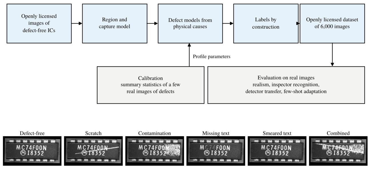
Figure 2.
Region and capture model for one openly licensed source image: (a) source image; (b) face mask F (pixels outside darkened); (c) marking mask T; (d) one defect-free capture produced by the capture model.
Figure 2.
Region and capture model for one openly licensed source image: (a) source image; (b) face mask F (pixels outside darkened); (c) marking mask T; (d) one defect-free capture produced by the capture model.

Figure 3.
Construction of the two surface defects on one defect-free capture at severity 0.75. Scratch: (a) the capture, (b) the drawn centerline (orange) and pressure envelope (white), (c) the density of the groove bundle with debris, (d) the opacity α after blurring by the point spread, (e) the defect image, (f) the exact mask (green), polygon (orange) and box (blue) taken from the renderer. Contamination: (g) the capture, (h) the shape kernel Σ, (i) the deposit field D after texture and fragmentation, (j) the opacity after the core-and-fringe ramp, (k) the defect image, (l) its annotation. The intermediate fields are defined on the face region and are shown in place on the whole image.
Figure 3.
Construction of the two surface defects on one defect-free capture at severity 0.75. Scratch: (a) the capture, (b) the drawn centerline (orange) and pressure envelope (white), (c) the density of the groove bundle with debris, (d) the opacity α after blurring by the point spread, (e) the defect image, (f) the exact mask (green), polygon (orange) and box (blue) taken from the renderer. Contamination: (g) the capture, (h) the shape kernel Σ, (i) the deposit field D after texture and fragmentation, (j) the opacity after the core-and-fringe ramp, (k) the defect image, (l) its annotation. The intermediate fields are defined on the face region and are shown in place on the whole image.
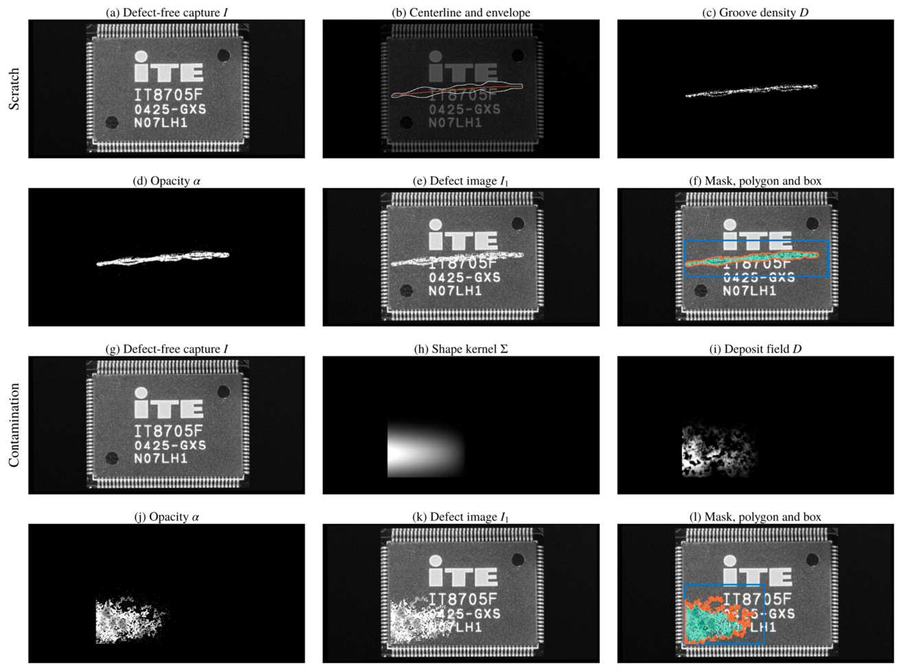
Figure 4.
Construction of the two marking defects on the same capture. Missing text: (a) the capture, (b) the selected character run Ξ, (c) the reconstructed background B under the run, (d) the dropout field η, (e) the defect image, (f) mask, polygon and box. Smeared text: (g) the capture, (h) the selected run, (i) its marking energy AΞ, (j) the redistributed energy
Figure 4.
Construction of the two marking defects on the same capture. Missing text: (a) the capture, (b) the selected character run Ξ, (c) the reconstructed background B under the run, (d) the dropout field η, (e) the defect image, (f) mask, polygon and box. Smeared text: (g) the capture, (h) the selected run, (i) its marking energy AΞ, (j) the redistributed energy
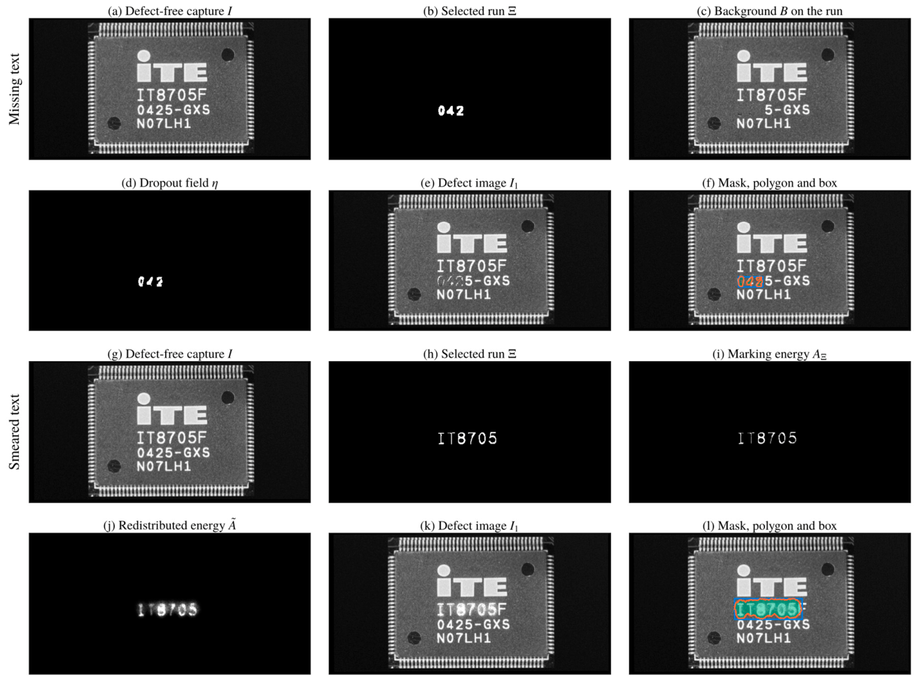
Figure 5.
Severity levels of the two marking defects on the same characters. (a) to (d): missing text at s = 0.25, 0.50, 0.75 and 1.00 (whole-character loss). (e) to (h): smeared text at the same four levels (defocused spot). Under each image, the affected run inside the blue box is shown enlarged. The levels are equally spaced in s, which enters the mechanisms through linear ramps, and not in perceived change: adjacent missing-text levels differ in the fraction of marking energy removed from the same characters, and adjacent smeared-text levels in the spot radius.
Figure 5.
Severity levels of the two marking defects on the same characters. (a) to (d): missing text at s = 0.25, 0.50, 0.75 and 1.00 (whole-character loss). (e) to (h): smeared text at the same four levels (defocused spot). Under each image, the affected run inside the blue box is shown enlarged. The levels are equally spaced in s, which enters the mechanisms through linear ramps, and not in perceived change: adjacent missing-text levels differ in the fraction of marking energy removed from the same characters, and adjacent smeared-text levels in the spot radius.
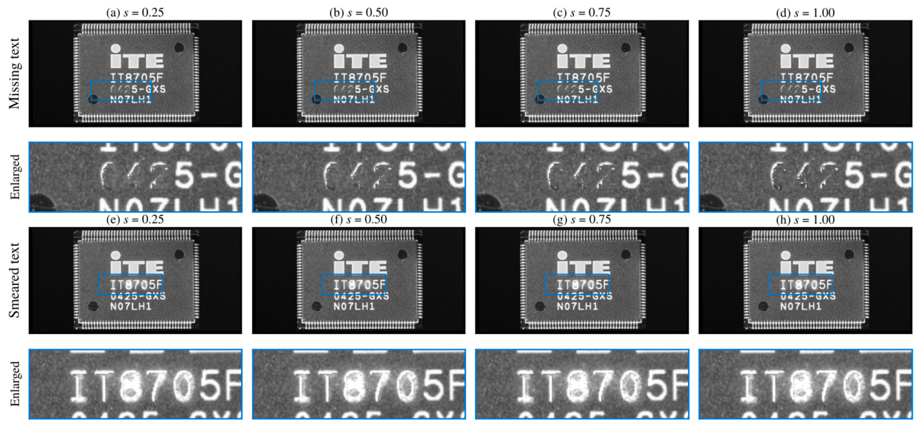
Figure 6.
Generated images for two source IC packages in the six classes (columns), shown without annotation, each with its exact defect mask in the row beneath (white).
Figure 6.
Generated images for two source IC packages in the six classes (columns), shown without annotation, each with its exact defect mask in the row beneath (white).
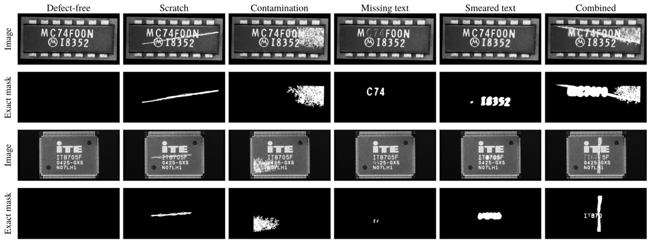
Figure 7.
Distance between generated and real defects relative to the real-pixel reference (patch blending, dashed line at 1), for the three methods that use no real defect pixels, on four distribution measures. Below 1 is closer to the real defects than a copy of real pixels. Absolute values and leave-one-image-out ranges are given in Table 7.
Figure 7.
Distance between generated and real defects relative to the real-pixel reference (patch blending, dashed line at 1), for the three methods that use no real defect pixels, on four distribution measures. Below 1 is closer to the real defects than a copy of real pixels. Absolute values and leave-one-image-out ranges are given in Table 7.
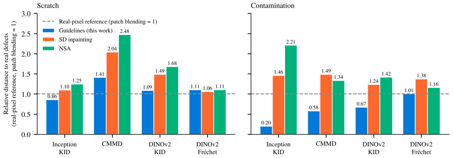
Figure 8.
The rule-based inspector of [1] on the synthetic test split (n = 715): all-class accuracy over the six image classes and binary accuracy (defective against defect-free), with the thresholds published for the reference IC package and with thresholds learned on the synthetic validation split.
Figure 8.
The rule-based inspector of [1] on the synthetic test split (n = 715): all-class accuracy over the six image classes and binary accuracy (defective against defect-free), with the thresholds published for the reference IC package and with thresholds learned on the synthetic validation split.
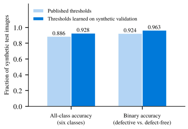
Figure 9.
Real defect images found by detectors trained on each synthetic dataset, at the operating point with at most 0.5 false boxes per defect-free image (mean of three seeds, error bars one sample standard deviation). Darker: scratch images of 6. Lighter, hatched: contamination images of 8. FA: false boxes per defect-free image. The guidelines images are shown under both evaluation protocols of Section 4.1: product-matched (all IC designs seen in training) and source-disjoint (no test design seen in training).
Figure 9.
Real defect images found by detectors trained on each synthetic dataset, at the operating point with at most 0.5 false boxes per defect-free image (mean of three seeds, error bars one sample standard deviation). Darker: scratch images of 6. Lighter, hatched: contamination images of 8. FA: false boxes per defect-free image. The guidelines images are shown under both evaluation protocols of Section 4.1: product-matched (all IC designs seen in training) and source-disjoint (no test design seen in training).
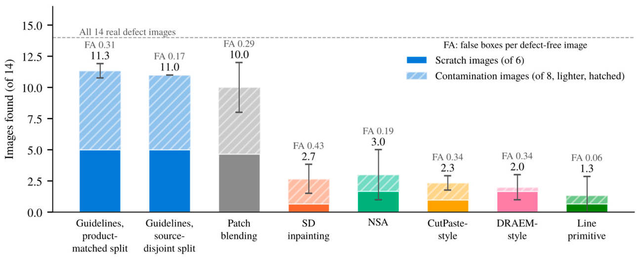
Figure 10.
Few-shot adaptation: the 14 held-out real defect images (boxes, filled when found) for the synthetic-trained detector fine-tuned with three or six real defect images, at the pre-fixed confidence of 0.25 (four folds, every real defect image held out once and used only for the final evaluation).
Figure 10.
Few-shot adaptation: the 14 held-out real defect images (boxes, filled when found) for the synthetic-trained detector fine-tuned with three or six real defect images, at the pre-fixed confidence of 0.25 (four folds, every real defect image held out once and used only for the final evaluation).
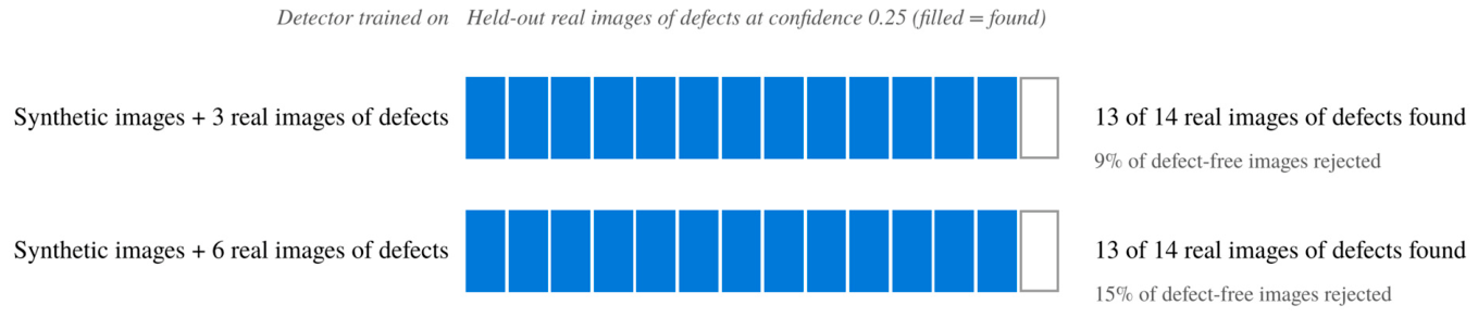
Figure 11.
Evidence for the two text-defect classes. (a) Fraction of synthetic test images flagged by the bad-symbol rule of the inspector of [1] with learned thresholds, for the missing-text and smeared-text classes and, as the false-positive rate, for the defect-free class. (b) Counterpart-referenced OCR error rate against severity level for the two classes, with bootstrap 95% intervals and the Spearman rank correlation per class.
Figure 11.
Evidence for the two text-defect classes. (a) Fraction of synthetic test images flagged by the bad-symbol rule of the inspector of [1] with learned thresholds, for the missing-text and smeared-text classes and, as the false-positive rate, for the defect-free class. (b) Counterpart-referenced OCR error rate against severity level for the two classes, with bootstrap 95% intervals and the Spearman rank correlation per class.
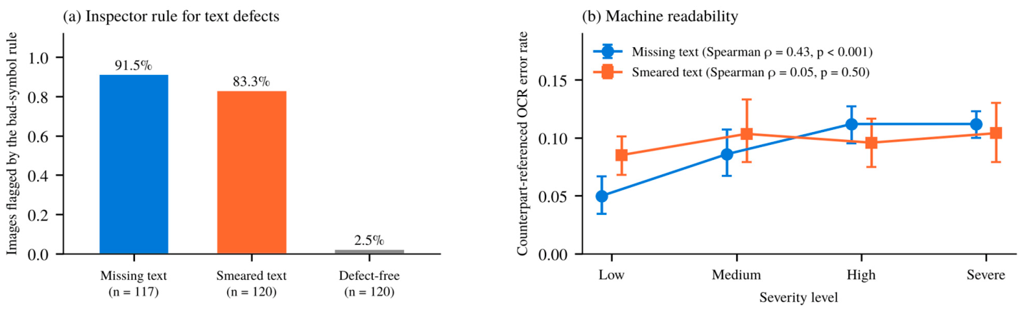
Table 1.
Approaches for generating synthetic images of defects compared by the properties that the marking inspection requires.
Table 1.
Approaches for generating synthetic images of defects compared by the properties that the marking inspection requires.
| Approach | Real defects needed | Specific defect | Exact labels | Marking defects | Checked against real | Main limitation |
|---|---|---|---|---|---|---|
| Generic anomaly synthesis [8,9,10,27] | no | no | yes | no | no | trains “not normal”, not a class |
| Copy-based, patch blending [1] | yes | yes | approximate | observed only | implicit | limited to observed defects |
| Generative models [11,12,28,29,30] | yes | learned | varies | no | separate | needs examples, limited control |
| Procedural, physics-based [16,17,18,19,31,32] | no | yes | yes | no | only in [31] | surface damage only |
| Physics-informed guidelines (this work) | statistics only | yes | yes | yes | by calibration | one IC package evaluated so far |
Table 2.
Public image datasets closest to the defective IC marking inspection, and the dataset provided in this paper.
Table 2.
Public image datasets closest to the defective IC marking inspection, and the dataset provided in this paper.
| Dataset | Domain | Images | Defect classes | Pixel masks | Marking defects | Origin |
|---|---|---|---|---|---|---|
| MVTec AD [63] | 15 objects and textures | 5,354 | 73 types | yes | no | real |
| VisA [64] | 12 objects, incl. PCBs | 10,821 | 4 to 9 per object | yes | no | real |
| Real-IAD [65] | 30 objects, five views | 151,050 | 8 types | yes | no | real |
| DsPCBSD+ [67] | bare PCB surfaces | 10,259 | 9 | boxes only | no | real |
| ICText [21] | IC package text | 100,152 characters | quality attributes | no | no | real |
| Dataset in [1] | one IC package | 58 | 5 | no | yes | real, not public |
| ICMarkingSynthetic (this work) | 40 IC packages | 6,000 | 4 defect types | yes, with polygons and boxes | yes | synthetic, from openly licensed images |
Table 3.
Composition of the ICMarkingSynthetic dataset.
| Item | Value |
|---|---|
| Source images | 40, Wikimedia Commons (38 CC BY-SA 4.0, 2 CC BY 2.0) |
| Images | 6,000 at 640 × 320 pixels, gray scale, 1,000 per class |
| Image-level classes | defect-free, scratch, contamination, missing text, smeared text, combined (two or three defects) |
| Defect detection classes | scratch, contamination, missing text, smeared text |
| Localization labels | boxes and polygons (full image and face crop), exact masks per defect, 6,757 visible instances |
| Source-disjoint split | 24 / 8 / 8 source images, 3,605 / 1,204 / 1,191 images |
| Product-matched split | by capture group, 4,569 / 716 / 715 images |
| Supplement | 467 cosmetic defect-free images (hard negatives) |
| Provenance per image | capture parameters, mechanism, severity, measurements, defect-free counterpart, seed, generator version |
Table 4.
Role of the real images in [1] in each experiment.
Table 4.
Role of the real images in [1] in each experiment.
| Experiment | Real images used | Form in which they are used | What they contribute |
|---|---|---|---|
| Calibration (Section 3.6) | 6 scratch, 8 contamination | summary statistics of descriptors | a few parameters of two profiles |
| Realism (Section 4.3) | 6 scratch, 8 contamination, 12 defect-free as source images | reference population, source images for generation | distance between generated and real defects |
| Inspection (Section 4.4) | none in the scoring set; the rules were designed on real images in [1], and the unspecified processing steps were fixed on the 47 real images before any synthetic image was scored | published thresholds, and thresholds learned on synthetic validation images | whether generated defects are recognized as intended |
| Detector transfer (Section 4.5) | all 47 | evaluation set; the fixed training protocol was chosen after a preliminary comparison on these images (Section 4.5), and the reported result is the evaluation after that choice | recall on real defects of a synthetic-only detector |
| Few-shot adaptation (Section 4.5) | 3 or 6 defective and 2 defect-free per fold | training data in folds that hold out every tested image | effect of a few real images |
| Text defects (Section 4.6) | none in the scoring set; the bad-symbol rule comes from [1] | not applicable | indirect evidence |
Table 5.
Evaluation coverage per image class. Calibration refers to the descriptor-based procedure of Section 3.6.
Table 5.
Evaluation coverage per image class. Calibration refers to the descriptor-based procedure of Section 3.6.
| Image class | Real reference images | Calibration | Realism measures (5.1) | Inspection (5.2) | Detector transfer (5.3) | Text tests (5.5) |
|---|---|---|---|---|---|---|
| Scratch | 6 | yes | yes | yes | yes | not applicable |
| Contamination | 8 | yes | yes | yes | yes | not applicable |
| Missing text | none | none | not possible | yes | not possible | inspection rule, OCR |
| Smeared text | none | none | not possible | yes | not possible | inspection rule, OCR |
| Combined | none | by its defects | not possible | yes | not possible (synthetic recoverability check only, Table S3) | by its defects |
| Defect-free | 33 | not applicable | source images | yes, as false-positive rate | yes, as false-alarm rate | false-positive rate |
Table 6.
Composition of the training sets of the detector comparison. All sets except patch blending use the same 40 source images, captures and source-disjoint split assignment. The product-matched guidelines rows are an additional experiment under the product-matched split. “Release” denotes the unchanged images of ICMarkingSynthetic.
Table 6.
Composition of the training sets of the detector comparison. All sets except patch blending use the same 40 source images, captures and source-disjoint split assignment. The product-matched guidelines rows are an additional experiment under the product-matched split. “Release” denotes the unchanged images of ICMarkingSynthetic.
| Training set | Images | Scratch and contamination images | Defect-free, missing-text and smeared-text images | Combined images | Real defect pixels |
|---|---|---|---|---|---|
| Guidelines, full release | 6,000 | 2,000, release | 3,000, release | 1,000, release | no |
| Guidelines, matched composition | 5,000 | 2,000, release | 3,000, release | none | no |
| Patch blending [1] | 1,275 | 1,242, real defect patches blended onto the 33 real defect-free images (1,100 scratch and 172 contamination instances) | 33 real defect-free images | none | yes |
| Stable Diffusion Inpainting [38] | 5,000 | 2,000, prompt-driven inpainting | 3,000, release | none | no |
| NSA [10] | 5,000 | 2,000, patches from other defect-free images | 3,000, release | none | no |
| CutPaste-style [8] | 5,000 | 2,000, pasted face and scar patches | 3,000, release | none | no |
| DRAEM-style [9] | 5,000 | 2,000, Perlin masks with external textures | 3,000, release | none | no |
| Line primitive | 5,000 | 2,000, straight bright lines | 3,000, release | none | no |
Table 7.
Realism of the defects generated on the reference IC package: distance between 50 generated images per class and the real defect images of the same class (6 scratch, 8 contamination), one script and one protocol for all the methods. Inception KID [51], CMMD on CLIP embeddings (× 1,000) [53], KID on DINOv2 features (× 1,000) and Fréchet distance on DINOv2 features [54]. Lower is closer to real. Brackets give the sensitivity range when each real image is left out in turn, not a confidence interval. The first row of each class is the real-pixel reference.
Table 7.
Realism of the defects generated on the reference IC package: distance between 50 generated images per class and the real defect images of the same class (6 scratch, 8 contamination), one script and one protocol for all the methods. Inception KID [51], CMMD on CLIP embeddings (× 1,000) [53], KID on DINOv2 features (× 1,000) and Fréchet distance on DINOv2 features [54]. Lower is closer to real. Brackets give the sensitivity range when each real image is left out in turn, not a confidence interval. The first row of each class is the real-pixel reference.
| Class | Images | Inception KID | CMMD | DINOv2 KID | DINOv2 Fréchet |
|---|---|---|---|---|---|
| Scratch | Reference: patch blending, real defect pixels [1] | 0.0196 [0.0113, 0.0329] | 0.090 [-0.001, 0.227] | 0.26 [0.13, 0.37] | 0.229 [0.223, 0.264] |
| Scratch | Guidelines (this work) | 0.0168 [0.0091, 0.0256] | 0.126 [0.021, 0.237] | 0.28 [0.16, 0.39] | 0.253 [0.247, 0.287] |
| Scratch | Stable Diffusion Inpainting [38] | 0.0215 [0.0112, 0.0367] | 0.183 [0.059, 0.280] | 0.39 [0.21, 0.54] | 0.243 [0.232, 0.281] |
| Scratch | NSA [10] | 0.0244 [0.0139, 0.0402] | 0.222 [0.105, 0.340] | 0.44 [0.26, 0.58] | 0.254 [0.240, 0.292] |
| Contamination | Reference: patch blending, real defect pixels [1] | 0.0300 [0.0250, 0.0385] | 0.267 [0.218, 0.361] | 0.38 [0.30, 0.48] | 0.207 [0.205, 0.228] |
| Contamination | Guidelines (this work) | 0.0061 [-0.0004, 0.0096] | 0.155 [0.098, 0.205] | 0.26 [0.19, 0.37] | 0.209 [0.206, 0.229] |
| Contamination | Stable Diffusion Inpainting [38] | 0.0438 [0.0349, 0.0561] | 0.398 [0.345, 0.456] | 0.47 [0.40, 0.58] | 0.285 [0.282, 0.310] |
| Contamination | NSA [10] | 0.0663 [0.0527, 0.0819] | 0.356 [0.271, 0.456] | 0.54 [0.46, 0.63] | 0.240 [0.234, 0.261] |
Table 8.
Transfer to the 47 real images at the operating point of Equation (10), with at most 0.5 false boxes per defect-free image, and at the pre-fixed confidence of 0.25. Mean ± sample standard deviation over three seeds, fixed YOLOv8n training protocol for all the methods. Image counts are the mean number of the 14 real defect images found per seed. FB denotes false boxes per defect-free image.
Table 8.
Transfer to the 47 real images at the operating point of Equation (10), with at most 0.5 false boxes per defect-free image, and at the pre-fixed confidence of 0.25. Mean ± sample standard deviation over three seeds, fixed YOLOv8n training protocol for all the methods. Image counts are the mean number of the 14 real defect images found per seed. FB denotes false boxes per defect-free image.
| Training images | Real defect pixels | Found / 14 | Scratch / 6 | Contamination / 8 | FB | Correct-class recall | Found / 14 at 0.25 | FB at 0.25 |
|---|---|---|---|---|---|---|---|---|
| Guidelines, full release, product-matched | no | 11.3 ± 0.6 | 5.0 ± 0.0 | 6.3 ± 0.6 | 0.31 ± 0.15 | 0.60 ± 0.04 | 11.3 ± 0.6 | 0.85 ± 0.42 |
| Guidelines, full release, source-disjoint | no | 11.0 ± 0.0 | 5.0 ± 0.0 | 6.0 ± 0.0 | 0.17 ± 0.22 | 0.60 ± 0.04 | 11.3 ± 0.6 | 1.29 ± 0.44 |
| Guidelines, matched 5,000, product-matched | no | 11.3 ± 1.2 | 5.0 ± 0.0 | 6.3 ± 1.2 | 0.19 ± 0.20 | 0.48 ± 0.04 | 11.7 ± 0.6 | 0.44 ± 0.15 |
| Guidelines, matched 5,000, source-disjoint | no | 11.0 ± 1.0 | 5.0 ± 0.0 | 6.0 ± 1.0 | 0.27 ± 0.11 | 0.55 ± 0.04 | 10.7 ± 1.2 | 0.61 ± 0.33 |
| Patch blending [1] | yes | 10.0 ± 2.0 | 4.7 ± 0.6 | 5.3 ± 1.5 | 0.29 ± 0.26 | 0.69 ± 0.15 | 8.0 ± 1.7 | 0.08 ± 0.06 |
| Stable Diffusion Inpainting [38] | no | 2.7 ± 1.2 | 0.7 ± 0.6 | 2.0 ± 1.0 | 0.43 ± 0.05 | 0.14 ± 0.07 | 7.3 ± 0.6 | 0.80 ± 0.02 |
| NSA [10] | no | 3.0 ± 2.0 | 1.7 ± 1.5 | 1.3 ± 0.6 | 0.19 ± 0.17 | 0.00 | 1.7 ± 0.6 | 0.36 ± 0.39 |
| CutPaste-style [8] | no | 2.3 ± 0.6 | 1.0 ± 0.0 | 1.3 ± 0.6 | 0.34 ± 0.11 | 0.00 | 2.0 ± 1.0 | 0.60 ± 0.12 |
| DRAEM-style [9] | no | 2.0 ± 1.0 | 1.7 ± 0.6 | 0.3 ± 0.6 | 0.34 ± 0.19 | 0.00 | 2.3 ± 0.6 | 0.51 ± 0.47 |
| Line primitive | no | 1.3 ± 1.5 | 0.7 ± 0.6 | 0.7 ± 1.2 | 0.06 ± 0.06 | 0.00 | 2.3 ± 0.6 | 0.67 ± 0.13 |
Disclaimer/Publisher’s Note: The statements, opinions and data contained in all publications are solely those of the individual author(s) and contributor(s) and not of MDPI and/or the editor(s). MDPI and/or the editor(s) disclaim responsibility for any injury to people or property resulting from any ideas, methods, instructions or products referred to in the content. |
© 2026 by the authors. Licensee MDPI, Basel, Switzerland. This article is an open access article distributed under the terms and conditions of the Creative Commons Attribution (CC BY) license (http://creativecommons.org/licenses/by/4.0/).
Copyright: This open access article is published under a Creative Commons CC BY 4.0 license, which permit the free download, distribution, and reuse, provided that the author and preprint are cited in any reuse.