

Submitted:
28 October 2026
Posted:
29 October 2026
You are already at the latest version
Abstract
A utility builds a reliability project only when the outage costs it saves its customers are larger than the cost of the project. In the United States, these outage costs usually come from one study of customer surveys. That study lists each cost in three ways: per outage, per kilowatt of average demand, and per kilowatt-hour of energy not served. Planners often treat the three numbers as the same cost written in different units. We show that the cost per outage equals the cost per kilowatt multiplied by the average demand of the typical survey customer. Using it therefore assumes that every customer in a group is the same size as that survey customer. We find the exact condition under which this hidden assumption changes which customer group a utility should protect first, when groups are ranked by their share of total outage cost. This condition does not depend on how long the outage lasts. In data for 1,989 U.S. utilities, the group with the largest outage cost changes at 29.0% of them. The total cost of a four-hour outage is also overstated at 66.8% of them. We close with reporting steps that make the hidden assumption easy to check.
Keywords:
distribution system planning
; customer interruption cost
; value of lost load
; value of service
; reli-ability worth
; benefit-cost analysis
; capital allocation
; rate case
1. Introduction
Every dollar that a utility spends on distribution reliability has to be justified by the outages it prevents. The dollar value of a prevented outage comes from a value-of-service study. In the United States, planners rely in practice on one publicly funded meta-analysis of customer surveys [1]. This study reaches them through a calculator built on it, and it is cited in rate filings across the country. As a result, its numbers set the benefit side of almost every reliability benefit-cost case that a U.S. utility makes.
Counting the outages that a project prevents is routine engineering work. It rests on standard reliability methods [2,3], on the indices defined in IEEE Std 1366 [4], and on the event recording practices of IEEE Std 1782 [5]. The weaker link in a reliability case is usually the dollar value placed on each outage.
The meta-analysis reports each of its results in three forms, which we call cost bases. For example, a four-hour outage costs a medium or large commercial and industrial (C&I) customer $39,458 per event. The same outage costs $48.40 per kilowatt of average demand, or $12.10 per kilowatt-hour of energy not served. The three numbers sit in neighboring columns of the same table. The study gives no advice on which one a planner should use, and neither does the guidance written for practitioners. As a result, most readers assume that the three columns describe the same cost in different units. On that reading, a planner can use whichever column fits the data at hand.
In this paper we show that this common reading is wrong and that it can be expensive. We build the argument in four steps, and each step leads to the next.
The first step, in Section 3, shows that the per-event figures are not a separate estimate at all. Each one equals the matching per-kilowatt figure multiplied by a single number. That number is the average demand of the typical customer whose survey answers were pooled to produce the class figure. This relationship follows from how the tables are built, and it matches the published values to within a fraction of a percent. For this reason, choosing the per-event basis is not a harmless choice of units. It quietly assumes that every customer in the class is the same size as that typical survey customer.
The second step, in Section 4, asks whether this hidden assumption can change a real decision. The decision we study is which customer class in a zone should receive reliability investment first. We rank the classes by their share of the zone’s total outage cost. If every class were misstated by the same factor, the zone total would change but the order of the classes would not. A planner who only compares projects within one class would then reach the same decision on either basis. The order can flip only when the classes are misstated by different factors. We give the exact range of per-kilowatt cost ratios between two classes inside which the flip happens. Two results from this step matter most in practice. First, the width of the range depends only on how differently the classes are misstated. Second, the range does not shrink as outages get longer, so the error does not fade in the long events that storm-hardening plans are built around.
The third step, in Sections 5 and 6, checks whether real systems fall inside this range. The study separates small from medium and large C&I customers at an annual consumption of 50,000 kWh/yr. This dividing line turns out to behave very badly in practice. When a customer crosses it, the cost per event goes up by a factor of about 24. At the same time, the cost per kilowatt goes down by a factor of about 15. So the two published bases do not even agree on the direction of the change. Across 1,989 U.S. utilities, the class with the largest share of outage cost changes with the basis at 29.0% of them.
In the fourth step, Section 7 follows the same effect through a model of one substation with three feeders. This model works at the level of detail that a capital plan uses. Section 8 then describes what a regulatory filing should report so that a reviewer can spot the problem.
1.1. Related Work and Contributions
The risk of carrying value-of-service numbers from one setting to another was noticed early. In a review of commonly raised issues, Sanghvi [6] observed that such data “can be used to any end.” He warned against “losing control of the data” and against conclusions drawn “well beyond its originally intended use.” However, every fix the author proposed was aimed at the people who design the surveys. None was aimed at the analyst who later takes a published number and applies it to customers who were never surveyed. Sanghvi also set aside the very variation that our analysis relies on. He noted that differences in customer makeup are “responsible for the bulk of the observed variation.” He then concluded that these differences “will always be present and should not be cause for concern.”
The closest earlier statement of our argument appears in the published discussion of that paper. There, Ender [7] asked why unserved energy should be the preferred measure. He pointed out that a different normalization “is likely to lead to different cost-benefit evaluations.” He also noted that the figure a customer gives depends on “the magnitude of my load.” The paper was published without a reply from the author, and the question was never answered. Thirty-five years later, per-event cost tables are still published and still applied to customers of any size.
More recent work has added a great deal of data, but it has not returned to the question of which basis to use. A meta-regression of 534 value-of-lost-load estimates from 47 countries [8] supports moving cost estimates between countries. It works only in dollars per kilowatt-hour and treats the mix of reporting units as a nuisance. Its advice is that future studies should use one common unit. The study does not look at differences in customer size within a class. It also reports that reliability indices do not predict the value of lost load in a statistically meaningful way. That finding runs against the practice built into the U.S. calculator.
Public outage data have also become much richer. A recent dataset from Pacific Northwest National Laboratory links county-level outage records across the United States with the severe weather and other events that occurred at the same time and place [9]. Data of this kind show how often and how widely customers lose power. The cost of each outage, however, still has to come from a value-of-service study. These cost figures also feed value-based planning methods that place sectionalizing switches, tie lines, and reclosers [10,11,12]. Such methods weigh the cost of new equipment against the outage cost it avoids. Any error in the cost basis therefore passes straight into those designs.
Against this background, the paper makes three contributions. First, it finds the exact relationship between two of the published bases. It shows that this relationship turns one of them into a statement about customer size (Proposition 1). Second, it derives the necessary and sufficient condition for that statement to reverse an investment ranking. It also shows that this condition does not depend on outage duration (Proposition 2 and Corollary 2). Third, it measures how often and how strongly the error appears across U.S. utilities. For this step it uses billing data from Form EIA-861 [13], and it needs no assumption about load factor.
2. The Cost Bases and What They Measure
To set up the analysis, consider a zone. For our purposes a zone is a protection section, meaning the group of customers who lose power when one protective device opens. The zone has nc customers of class c, and their mean demand is .
The published tables also give a cost per kilowatt-hour of unserved energy. Apart from rounding, however, that figure equals the cost per kilowatt divided by the outage duration h. This means it grows with customer size in the same way as the per-kilowatt figure, and it ranks the classes in the same order. For this reason, only two bases need to be compared. For an outage of duration h, these two bases give the zone costs
Here, is the published outage cost per event for one customer of class c, in dollars per customer. In the same way, is the published outage cost per kilowatt of average demand for class c, in dollars per kilowatt. The quantities Zev(h) and ZkW(h) are the total outage costs of the zone on the per-event and per-kilowatt bases, in dollars. The difference between these two expressions is real and not just a matter of notation. In (2), the size of each customer enters directly through . In (1), customer size does not appear at all. A basis that never mentions customer size cannot be neutral about size, so it must be carrying a size somewhere. The next section shows where that size is hidden.
Before that, one more number from the study needs attention. For each class, the meta-analysis reports the mean annual consumption of the typical survey customer [1], whom we call the reference customer. We write this annual consumption as for class c. These values are 13,351 kWh/yr for residential customers and 19,214 kWh/yr for small C&I customers. For medium and large C&I customers, the value is 7,140,501 kWh/yr. The two C&I classes are split at an annual consumption of 50,000 kWh/yr. The medium and large reference customer sits far above the floor of its own class. The class starts at 50,000 kWh/yr, but its average survey respondent uses 143 times that amount. In other words, very large industrial loads dominate this class.
3. The Per-Event Cost Hides a Fixed Customer Size
As noted at the end of Section 2, the value-of-service study [1] reports the mean annual consumption of the survey respondents in each class. We call a customer of that size the reference customer of the class. Dividing each value by the 8,760 hours in a year gives the reference customer’s mean demand, . This demand is 1.52 kW for residential customers and 2.19 kW for small C&I customers. For medium and large C&I customers, it is 815 kW. The result below shows that this one number per class links the two published bases.
Proposition 1.
For each class c and each duration h, the published per-event and per-kilowatt figures satisfy
where is the average demand of the reference customer for class c. The per-event column adds no information beyond the per-kilowatt column and . Using the per-event basis is the same as using the per-kilowatt basis while assuming that for every customer in the class.
Proof.
A survey asks each respondent how much money an outage would cost them. The per-event figure for a class is built from these losses across all respondents. The per-kilowatt figure is the same quantity divided by the respondents’ mean demand. The two figures differ by exactly that mean demand, which equals by the definition of average demand. Substituting (3) into (1) gives , which is (2) with replaced by . □
Because both columns are published, (3) is easy to check. Figure 1 plots the ratio for all three classes at all six durations in the tables. This ratio has units of kilowatts, so it can be read as an implied demand. The figure compares it with , which we compute separately from the reported reference consumption. In every case, the ratio stays flat across durations and lands on the predicted value. The colors in this figure and in the later ones come from a palette that stays readable for people with color vision deficiency [14].
Table 1 lists the numbers behind this check. The demand recovered from the tables matches the separately computed reference demand very closely. The gap is 0.002% for small C&I customers, 0.02% for medium and large C&I customers, and 0.4% for residential customers. These small gaps come from rounding in the published tables. They are largest for residential customers because that per-event column is printed with only two or three significant figures. Across the six durations, the recovered value varies by a coefficient of variation of 0.02%, 0.09%, and 1.2% for the three classes, respectively.
This result has two direct consequences, and they shape the rest of the paper.
First, the per-event basis gives the right cost only for customers of about the same size as the reference customers. When the costs are applied to customers of a different size, the error grows in direct proportion to the size gap. Let Ec be the observed mean annual consumption of the class c customers on the system being studied, so that their mean demand is . To measure the size gap, we define the size mismatch factor
so the per-event basis misstates the cost of class c by the factor 1/γc. The right-hand form of (4) is the useful one in practice. Average demand and annual consumption differ only by a fixed constant. As a result, γc can be computed from actual consumed energy alone, meaning the metered annual kilowatt-hours that utilities already record for billing. No assumption about load factor, coincidence, or the ratio of peak to average demand is needed.
Second, and less obviously, this error is not a uniform bias that a planner could cover with a safety margin. The error differs from one class to another, so it distorts the comparison between classes. That comparison is exactly what decides where storm-hardening money goes.
4. When the Hidden Size Changes a Decision
Consider two classes a and b that compete for the same capital. On the per-kilowatt basis, the ratio of their contributions to the zone’s outage cost is
and class a is served first when .
Proposition 2.
On the per-event basis, the same ratio becomes
and the two bases rank the two classes differently if and only if
Proof.
Substituting (3) into (5), with replaced by , gives , which is (6). The two rankings differ exactly when and fall on opposite sides of one. If γb > γa, this happens when , and if γb < γa, it happens when . Putting the two cases together gives the condition in (7). □
Corollary 1.
If γa = γb, the range in (7) is empty and no reversal can happen for any value of . In that case the two bases differ only by a common factor. For a reversal to happen, the two classes must be misstated by different amounts.
This corollary matters most in practice because it answers the most natural defense of the per-event basis. A planner who suspects that the reference customer is too large might expect the error to inflate every class equally. On that view, the error would simply cancel out. It does not cancel, because the reference customers of the three classes draw 1.52, 2.19, and 815 kW. These sizes sit in very different places compared with the customers on any real feeder. As a result, γc differs across classes by orders of magnitude, and the range in (7) is wide.
Corollary 2.
The range in (7) does not depend on h.
Proof.
The factor γc depends only on consumption. By (6), the ratio contains no term in duration. □
Corollary 2 answers a second natural defense, which holds that the basis error matters only for short outages and fades for the long events that drive storm-hardening plans. We computed directly from the published tables at each of the six durations. It varies by only 0.25% for the pair of C&I classes and by 3.3% for pairs that include residential customers. The larger spread again comes from the coarse rounding of the residential per-event column. Within the precision of the published numbers, this ratio does not change with duration.
4.1. Numerical Check
We also tested Proposition 2 with a Monte Carlo study of 200,000 random cases. Each case used one pair of classes and one of the six durations. Customer counts were drawn evenly from [1,5000] for each class in the pair. Mean demands were drawn on a log scale over three orders of magnitude, from 0.1 kW to 1000 kW. With the exact form of (3), condition (7) correctly predicted whether a reversal occurred in all 200,000 cases. We then repeated the test with the rounded published tables. In that test, the only cases the condition missed fell within a 4% band around either edge of the range. In this band, rounding in the tables makes the edge uncertain. Overall, a reversal occurred in 38.95% of the sampled cases.
Figure 2 draws the condition as a map and places real utilities on it. The shaded wedge between and is where the ranking reverses. Each point is one U.S. utility, placed using data from Form EIA-861 [13]. Class a is the utility’s commercial sector, and class b is its industrial sector. Each sector is assigned to the small C&I class or to the medium and large C&I class according to its own mean annual consumption. A large share of utilities falls inside the wedge, which points ahead to the results in Section 6.
5. What Happens at the Class Boundary
Before turning to utility data, it helps to look at one case that needs no particular system. This case is the boundary between the two C&I classes.
The two classes are separated at 50,000 kWh/yr, which equals an average demand of 5.71 kW. Consider two customers on either side of this line. One uses 49,999 kWh/yr, and the other uses 50,001 kWh/yr. For any engineering purpose, these two customers are the same. Figure 3 shows the cost of an outage for each of them, on both bases and at all six durations.
On the per-event basis, crossing the line raises the customer’s cost by a factor of 17.9 to 31.4, depending on duration. The average increase is a factor of 24.2. On the per-kilowatt basis, the same move lowers the cost by a factor of 15.3 on average. These are not two estimates of the same quantity that happen to differ in size, because they point in opposite directions. Under one basis, the small C&I class is the cheaper one to interrupt. Under the other basis, it is the more expensive one.
Proposition 1 explains why the two bases behave so differently at this line. Crossing the line does not change the customer. It does change the reference customer that the per-event figure quietly assumes. That reference customer jumps by a factor of 372, from the small C&I reference customer at 2.19 kW to the medium and large C&I reference customer at 815 kW. The per-event column carries this jump with it, but the per-kilowatt column does not. Instead, the per-kilowatt column reports the real survey finding that small C&I customers lose a lot of money per kilowatt of demand. The disagreement in direction is simply the jump in γ at the boundary made visible.
The same reasoning also shows which basis is easier to defend. The per-kilowatt figure divides each class’s survey losses by the respondents’ own average demand. It can therefore be scaled to any customer whose demand is known. The per-event figure is that same quantity multiplied back by the average demand of the reference respondent. It is accurate only for customers of about that size.
6. How Often This Happens at U.S. Utilities
The results in Sections 3 to 5 are analytical. Whether they matter in practice depends on how far real customers are from the reference customers. This section answers that question with data for the whole population of U.S. utilities.
6.1. Data and Checks
We use the “Sales to Ultimate Customers” file of Form EIA-861 for the year 2014 [13]. This was the most recent year for which we had a machine-readable file at the utility level. The file reports revenue, sales in megawatt-hours, and customer counts by utility, state, and sector. We keep the fifty states and the District of Columbia. As the form’s own instructions require, we add up only parts A, B, and D. These parts are types of service rather than data columns. Part A is bundled energy and delivery service from utilities, and part B is energy-only service. Part D is bundled service from retail power marketers. Part C covers delivery-only service and would count the same customers twice. After this filter, 2,060 utilities remain in the data set.
This filter can be checked against independent published totals. We added up the kept records to the national level. They reproduce, digit for digit, the six matching totals published in the Electric Power Annual [15]. For the residential sector, these totals are 1,407,208,311 MWh and 128,680,416 customers. For the commercial sector, they are 1,352,158,263 MWh and 17,853,995 customers. For the industrial sector, they are 997,576,138 MWh and 839,212 customers. We report this check because every γ in the paper is a ratio of sales to customers. An error in the filter would bias all of them without leaving any visible sign. For example, wrongly including part C would add 19.8% to commercial sales but only 10.7% to commercial customers. That change would shift the mean consumption, and therefore γ, of every affected utility. Matching the published totals exactly rules out this kind of error.
Two mapping choices are also needed, and we state them openly. EIA reports three sectors, namely residential, commercial, and industrial. The value-of-service study, on the other hand, defines three classes (see Figure 1), and two of them are separated by a consumption threshold. We assign the residential sector to the residential class. We then compare each utility’s own mean annual use in its commercial and industrial sectors with the value-of-service study’s 50,000 kWh/yr threshold. This comparison places each sector in the small C&I class or in the medium and large C&I class. This assignment relies on the value-of-service study’s own definition rather than on an outside one. Because a sector average is compared with a threshold, each sector of a utility lands in a single class. This holds even when the customers in that sector fall on both sides of the line. Section 9 discusses which way this choice biases the results.
6.2. How Far Are Real Customers from the Reference Customer?
At the national level, residential customers turn out to be close to their reference customer. Customers in the other sectors are far from theirs. The average U.S. residential customer used 10,936 kWh/yr in 2014, which gives γ = 0.819. The per-event basis therefore overstates residential outage cost by 22%. The average commercial customer used 75,734 kWh/yr. This is just above the 50,000 kWh/yr line, so this customer falls in the medium and large class. It is then compared with a reference customer that uses 7.14 GWh/yr. The result is γ = 0.0106, and the per-event basis overstates its cost by a factor of 94.3. The average industrial customer used 1.19 GWh/yr. This gives γ = 0.167 and an overstatement of 6.0 times.
The spread across utilities, shown in Figure 4, tells us more than these national averages. Residential values of γ cluster tightly near one, with a median of 0.911. In addition, 93% of utilities fall within a factor of two of the residential reference customer. That is a reasonable working test of whether a cost transfers well from the survey to a utility. Commercial and industrial values do not cluster at all. Their medians are 0.677 and 0.554, but only 34% and 33% of utilities fall within a factor of two. The commercial values form two separate peaks with a wide gap between them. The industrial values are skewed to the left, with a single peak and a long tail toward small values of γ.
The two commercial peaks are the boundary effect of Section 5 showing up in real data. Consider a utility whose average commercial customer falls just below the threshold. That utility is compared with a 19,214 kWh/yr reference customer and lands near γ ≈ 1. Now consider a utility whose average commercial customer falls just above the threshold. That utility is compared with a 7.14 GWh/yr reference customer and lands near γ ≈ 0.01. The customers of these two utilities may differ only slightly in size. Yet they are compared with reference customers whose sizes differ by a factor of about 370. The gap in Figure 4 comes from the class definition itself. Its width of two orders of magnitude is also the width of the reversal range that decides whether a ranking survives a change of basis, according to Proposition 2.
6.3. Effect on Total Cost and on Investment Priority
We next compute the cost of a four-hour outage of each utility’s entire customer base on both bases. For this we use (1) and (2) with the utility’s own class mix and its own mean demands. Four hours is the middle duration in the tables and is typical of a sustained distribution outage. By Corollary 2, the conclusion about which class to serve first does not depend on this choice. Not every utility has two classes to compare. Of the 2,060 utilities, 71 serve only one sector (29 industrial only, 20 residential only, and 19 commercial only) or report no customers (3). Removing these utilities leaves 1,989 for the analysis that follows.
Figure 5 and Table 2 summarize the results. We look first at the effect of the basis on total cost. The per-event basis gives a higher total than the per-kilowatt basis at 66.8% of utilities. For each utility, we divide its per-event total by its per-kilowatt total. Across utilities, this ratio has a median of 4.91 and a ninetieth percentile of 79.7. At the tenth percentile, the per-event total is only about half the per-kilowatt total. For this reason, a planner cannot treat the choice of basis as a safe, conservative choice in either direction. The per-event basis overstates the cost for some utilities and understates it for others. There is no way to tell which without computing γ.
For planning, the effect on investment priority matters more than the effect on totals. By investment priority we mean the choice of which customer class receives reliability investment first. The class with the largest share of outage cost changes with the basis at 576 of the 1,989 utilities, or 29.0%. These reversals run in both directions and are close to balanced. Commercial replaces industrial as the leading class at 295 utilities, and industrial replaces commercial at 265. This near balance tells us something useful about the nature of the error. A bias that always ran one way could be fixed with a correction factor. A reversal that runs both ways cannot be fixed in this way, because its direction depends on each utility’s own class mix.
7. Case Study: A Substation with Three Feeders
The utility-level analysis shows how often the error occurs. However, it averages over the zones that planners actually work with. For that reason, this section follows the effect through one distribution model at the level of detail that a capital plan uses.
The test system is an OpenDSS model built from real feeder data for a distribution substation somewhere in the United States. Its geographic location is masked, so the model identifies no particular utility or service area. The substation has three radial feeders and serves 4,168 customers. Each load in the model has an annual load shape. The name of that load shape identifies the load as residential, small commercial, or medium commercial. We use these names to assign each load to one of the three classes. We then measure the mean demand of each class from the model itself. The model has 3,323 residential customers at 3.67 kW and 549 small C&I customers at 4.00 kW. It also has 296 medium and large C&I customers at 31.26 kW.
The last of these numbers deserves a closer look. An average demand of 31.26 kW is a sizable commercial customer on a distribution feeder. It is nearly eight times the size of the average small C&I customer on the same system. So the class assignment in the model is not obviously wrong. However, the reference customer for this class draws 815 kW. The medium and large customers in the model are roughly 47 times smaller than the customer whose survey answers set their per-event cost.
Table 3 gives the cost of a four-hour outage of the whole substation on both bases. The model reports demand rather than annual energy. Converting demand to annual consumption requires a load factor. For this reason, we report the results at two load factors to show which parts of the outcome depend on that choice.
The reversal in priority is large, and Figure 6 shows it directly. On the per-event basis, medium and large C&I customers appear to carry 91.7% of the substation’s outage cost. A plan built on that number would harden their laterals first. On the per-kilowatt basis, the same customers carry only 18.6%, while small C&I customers carry 78.2%. In other words, the two bases point the utility toward different hardening work.
The role of the load factor is worth spelling out, since it shows how much of this result depends on an assumption. The load factor is needed only to convert the model’s demand values into annual consumption, on which γ is defined. It scales every class by the same amount. By Corollary 1, it therefore cannot create or remove a reversal. The cost shares in Table 3 are the same at both load factors, just as the corollary predicts. What the load factor does change is the size of the gap between the totals. That gap moves from 9.63 times to 5.30 times. The conclusion about which class to serve first is the one that decides where capital goes. This conclusion does not depend on the only assumption in the case study. It is also why the utility-level analysis of Section 6 is the stronger evidence, because billing energy needs no load factor at all.
8. What Planners and Regulators Can Do
None of these findings calls for a new cost model. The per-kilowatt column of the existing meta-analysis already works well for planning. The trouble is that a neighboring column carries an assumption that cannot be seen where the number is used. Current practice also gives a reviewer no way to detect it. With this in mind, we propose three requirements for planning studies and regulatory filings.
8.1. Compute and Publish γc Before Using Any Per-Event Figure
Equation (4) needs only one number per class, and every utility already has it. That number is the mean annual consumption from the utility’s billing records. This size check costs little, needs no modeling, and settles the question. We suggest that per-event figures be reported only when γc lies between 0.5 and 2 for every class c in the analysis. We also suggest that γc be published next to the cost whenever per-event figures are used. Under this rule, the residential class would usually pass and the C&I classes would usually fail. That is the right outcome, given what the data show.
8.2. Report the Class with the Largest Cost Share on Both Bases
A reversal depends on each utility’s own class mix (Proposition 2). It can also run in either direction (Section 6). For these reasons, no default basis is safe and no correction factor exists. A filing should report which class carries the largest share of outage cost on both bases. This makes the sensitivity visible at almost no cost. Where the two bases agree, the ranking can be relied on. Where they disagree, the disagreement is itself the finding. In that case, the per-kilowatt result should decide the matter, for the reason given in Section 5.
8.3. Treat the Class Boundary as a Modeling Decision Rather than a Table Lookup
A customer near 50,000 kWh/yr can be assigned costs that differ by more than an order of magnitude. The size and direction of the difference depend on the basis and on which side of the line the customer falls. Where a meaningful share of a zone’s load sits near this line, both class assignments should be run. The difference between them should then be reported. This is the case in which our own sector-average mapping is weakest. It is also the case in which a real planning study needs the most care.
More broadly, the problem is not limited to one survey study. Any cost table stated per customer rather than per unit of demand carries a hidden customer size. Propositions 1 and 2 apply to such tables as well. Outage cost estimates are now moving toward newer proprietary studies built on new survey panels. The reference customers will change, but the structure of the problem will not. The questions to ask of any new table stay the same. The reference sizes need to be published so that those questions can be answered.
9. Limitations
The empirical results of this paper have four main limitations, and we describe each of them in turn.
The first and most important limitation is that we compare a sector average with the class threshold. As a result, the commercial sector and the industrial sector of each utility are each placed in a single class. In reality, the customers in a sector fall on both sides of the line. This simplification hides the variation within each sector. That variation would widen the spread of γ and with it the reversal range. We therefore expect the true share of utilities with a reversal to be higher than the 29.0% we report. Our estimate should be read as a lower bound. Billing data at the customer level would settle the question. Such data would also allow the boundary treatment recommended in Section 8.
The second limitation has to do with the age of the data. The machine-readable utility file available to us is for 2014. The class definitions and reference sizes come from a study published in 2015 that uses earlier survey data. The two sources describe roughly the same period, as they should. Still, the results do not describe today’s utilities. Since 2014, residential use per customer has fallen slightly, while commercial use has risen. Both trends push commercial γ further from one. We would expect the 2014 results to understate today’s share of reversals, but we have not checked this at the utility level.
Third, all costs are in the published 2013 dollars and have not been adjusted for inflation. Such an adjustment multiplies both bases by the same factor. As a result, it changes no ratio, share, or reversal reported here. It would affect only the dollar totals in Table 3 and Table 4.
Fourth, the case study is based on a feeder model and not on a utility’s customer and billing records. As a result, the mean demand of each class comes from the load values in the model rather than from metered consumption. We use the case study only to show how the effect plays out at one substation. The general conclusions of the paper rest on the utility-level analysis in Section 6.
Beyond these four points, our results inherit two limits of the underlying data. The published cost functions stop at 16 hours, while restoration after major events often takes several days [16]. Any cost for a multi-day outage extends the model beyond the range it was fitted to. In addition, the regional adjustment of these costs rests on weak ground, because region and study year are mixed together in the source data. Neither limit affects our argument about the cost basis, since both bases share them equally.
10. Conclusions
The cost bases in a value-of-service study are not interchangeable ways of stating one number. We showed that the per-event basis equals the per-kilowatt basis multiplied by the average demand of the reference customer. This relationship matches the published tables to within a fraction of a percent. Choosing the per-event basis therefore quietly assumes that every customer in a class draws that reference demand. We then derived the exact condition under which this assumption reverses an investment ranking rather than just rescaling it. We also showed that a reversal requires the classes to be misstated by different amounts, and that it does not fade as outages get longer.
Real systems meet this condition far more often than one might expect. Across 1,989 U.S. utilities, the class with the largest share of outage cost changes with the basis at 29.0% of them. For a four-hour outage, the per-event basis gives a higher total cost at 66.8% of utilities, with a median ratio of 4.91. Because reversals run in both directions, no correction factor can repair the choice of basis. The class boundary at 50,000 kWh/yr is even worse than imprecise, since the two published bases disagree about the direction of its effect.
Fixing the problem needs neither new surveys nor a new cost model. First, the ratio of observed mean consumption to the reference customer’s consumption should be computed and published before any per-event figure is used. Second, the class with the largest share of outage cost should be reported on both bases, so that a reviewer can see whether the ranking holds. Both steps use data that utilities already hold and need no new modeling. Without them, a capital plan may end up directed by a customer who is not on the system at all.
Author Contributions
Conceptualization, R.K.B. and K.S.A.; methodology, R.K.B.; software, R.K.B.; validation, R.K.B., K.S.A. and N.G.; formal analysis, R.K.B. and N.G.; investigation, R.K.B.; data curation, R.K.B.; writing, original draft preparation, R.K.B.; writing, review and editing, K.S.A., V.C. and N.G.; visualization, R.K.B.; supervision, V.C. and N.G. All authors have read and agreed to the published version of the manuscript.
Funding
This research received no external funding.
Institutional Review Board Statement
Not applicable.
Informed Consent Statement
Not applicable.
Data Availability Statement
The utility data used in this study are published by the U.S. Energy Information Administration as Form EIA-861 and are available online at https://www.eia.gov/electricity/data/eia861/. The interruption cost figures come from the Lawrence Berkeley National Laboratory report cited in this article. The scripts that reproduce every number reported here are available from the corresponding authors on reasonable request.
Acknowledgments
The authors thank the U.S. Energy Information Administration for maintaining Form EIA-861 as a public resource, without which the utility-level analysis in Section 6 would not have been possible.
Conflicts of Interest
The authors declare no conflicts of interest.
Nomenclature
The following symbols and abbreviations are used in this manuscript:
| c | Customer class index (residential, small C&I, or medium and large C&I) |
| a, b | Two customer classes being compared |
| h | Outage duration, hours |
| nc | Number of customers of class c in a zone |
| Published outage cost per event, $/customer | |
| Published outage cost per kW of average demand, $/kW | |
| Ec | Observed mean annual consumption of class c, kWh/yr |
| Mean annual consumption of the reference customer of class c, kWh/yr | |
| γc | |
| Zev(h) | Total outage cost of a zone, per-event basis, $ |
| ZkW(h) | Total outage cost of a zone, per-kW basis, $ |
| Ratio of the outage cost of class a to that of class b, per-kW basis | |
| Ratio of the outage cost of class a to that of class b, per-event basis | |
| C&I | Commercial and industrial |
| EIA | U.S. Energy Information Administration |
References
- Sullivan, M.J.; Schellenberg, J.; Blundell, M. Updated Value of Service Reliability Estimates for Electric Utility Customers in the United States; Report LBNL-6941E; Lawrence Berkeley National Laboratory: Berkeley, CA, USA, 2015. [Google Scholar]
- Billinton, R.; Allan, R.N. Reliability Evaluation of Power Systems, 2nd ed.; Springer: New York, NY, USA, 1996. [Google Scholar]
- Brown, R.E. Electric Power Distribution Reliability, 2nd ed.; CRC Press: Boca Raton, FL, USA, 2008. [Google Scholar]
- IEEE Std 1366-2022; IEEE Guide for Electric Power Distribution Reliability Indices. IEEE: New York, NY, USA, 2022.
- IEEE Std 1782-2022; IEEE Guide for Collecting, Categorizing, and Utilizing Information Related to Electric Power Distribution Interruption Events. IEEE: New York, NY, USA, 2022.
- Sanghvi, A.P. Measurement and application of customer interruption costs/value of service for cost-benefit reliability evaluation: Some commonly raised issues. IEEE Trans. Power Syst. 1990, 5, 1333–1344. [Google Scholar] [CrossRef]
- Ender, R.C. Discussion of “Measurement and application of customer interruption costs/value of service for cost-benefit reliability evaluation: Some commonly raised issues”. IEEE Trans. Power Syst. 1990, 5, 1344. [Google Scholar] [CrossRef]
- Jin, T. A meta-analysis of outage cost for value-based reliability planning. Energy Strategy Rev. 2025, 62, 101975. [Google Scholar] [CrossRef]
- She, B.; Adetola, V.; Yun, J.Y. Event-Correlated Outage Dataset in America; Pacific Northwest National Laboratory: Richland, WA, USA, 2024; Available online: https://catalog.data.gov/dataset/event-correlated-outage-dataset-in-america (accessed on 22 October 2026).
- Abiri-Jahromi, A.; Fotuhi-Firuzabad, M.; Parvania, M.; Mosleh, M. Optimized sectionalizing switch placement strategy in distribution systems. IEEE Trans. Power Deliv. 2012, 27, 362–370. [Google Scholar] [CrossRef]
- Jooshaki, M.; Karimi-Arpanahi, S.; Lehtonen, M.; Millar, R.J.; Fotuhi-Firuzabad, M. Reliability-oriented electricity distribution system switch and tie line optimization. IEEE Access 2020, 8, 130967–130978. [Google Scholar] [CrossRef]
- Ghorbani-Juybari, M.Z.; Gholizade-Narm, H.; Damchi, Y. Optimal recloser placement in distribution system considering maneuver points, practical limitations, and recloser malfunction. Int. Trans. Electr. Energy Syst. 2022, 2022, 5062350. [Google Scholar] [CrossRef]
- U.S. Energy Information Administration. Form EIA-861, Annual Electric Power Industry Report: Sales to Ultimate Customers, 2014. Available online: https://www.eia.gov/electricity/data/eia861/ (accessed on 22 October 2026).
- Wong, B. Points of view: Color blindness. Nat. Methods 2011, 8, 441. [Google Scholar] [CrossRef] [PubMed]
- U.S. Energy Information Administration. Electric Power Annual 2014, Tables 2.1 and 2.2. Available online: https://www.eia.gov/electricity/annual/ (accessed on 22 October 2026).
- Eto, J.H.; LaCommare, K.H.; Sohn, M.D.; Caswell, H. Evaluating the performance of the IEEE Standard 1366 method for identifying major event days. IEEE Trans. Power Syst. 2017, 32, 1327–1333. [Google Scholar] [CrossRef]
Figure 1.
Implied demand taken from two neighboring columns of the published tables (markers). The dotted lines show the reference customer’s average demand , computed separately from the reported reference consumption. The ratio stays flat across durations and matches the predicted value for all three classes over nearly three orders of magnitude. The per-event column is therefore the per-kilowatt column multiplied by a customer size.
Figure 1.
Implied demand taken from two neighboring columns of the published tables (markers). The dotted lines show the reference customer’s average demand , computed separately from the reported reference consumption. The ratio stays flat across durations and matches the predicted value for all three classes over nearly three orders of magnitude. The per-event column is therefore the per-kilowatt column multiplied by a customer size.
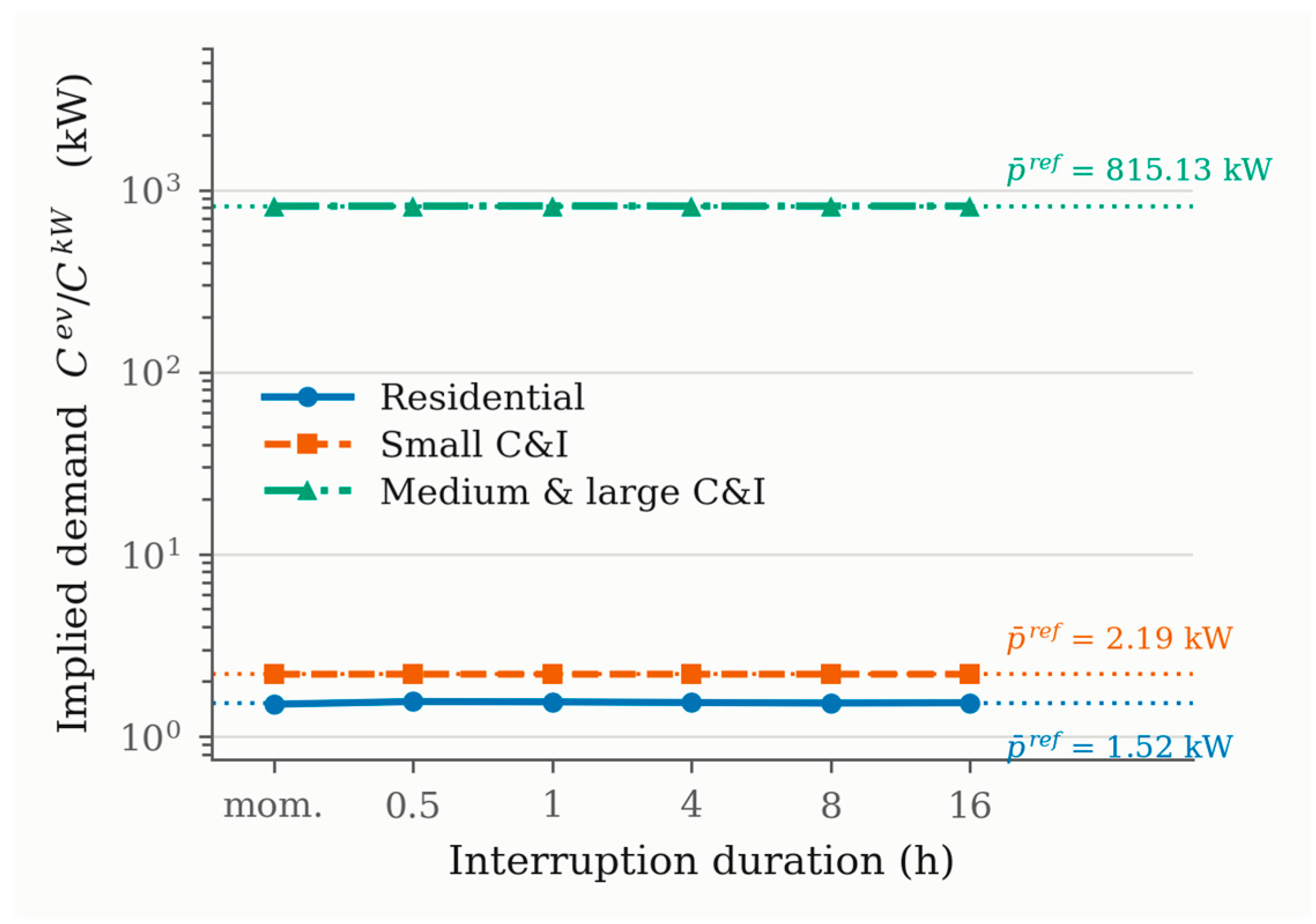
Figure 2.
Reversal condition (7) drawn as a map. The shaded wedge between (dashed line) and (solid line) is where the two bases rank the two classes differently. Each point is a U.S. utility from Form EIA-861, placed by the data for its own commercial and industrial sectors for a four-hour outage. The wedge is wide because γ differs across classes by orders of magnitude. It closes only on the diagonal, where the two classes are misstated by the same amount.
Figure 2.
Reversal condition (7) drawn as a map. The shaded wedge between (dashed line) and (solid line) is where the two bases rank the two classes differently. Each point is a U.S. utility from Form EIA-861, placed by the data for its own commercial and industrial sectors for a four-hour outage. The wedge is wide because γ differs across classes by orders of magnitude. It closes only on the diagonal, where the two classes are misstated by the same amount.
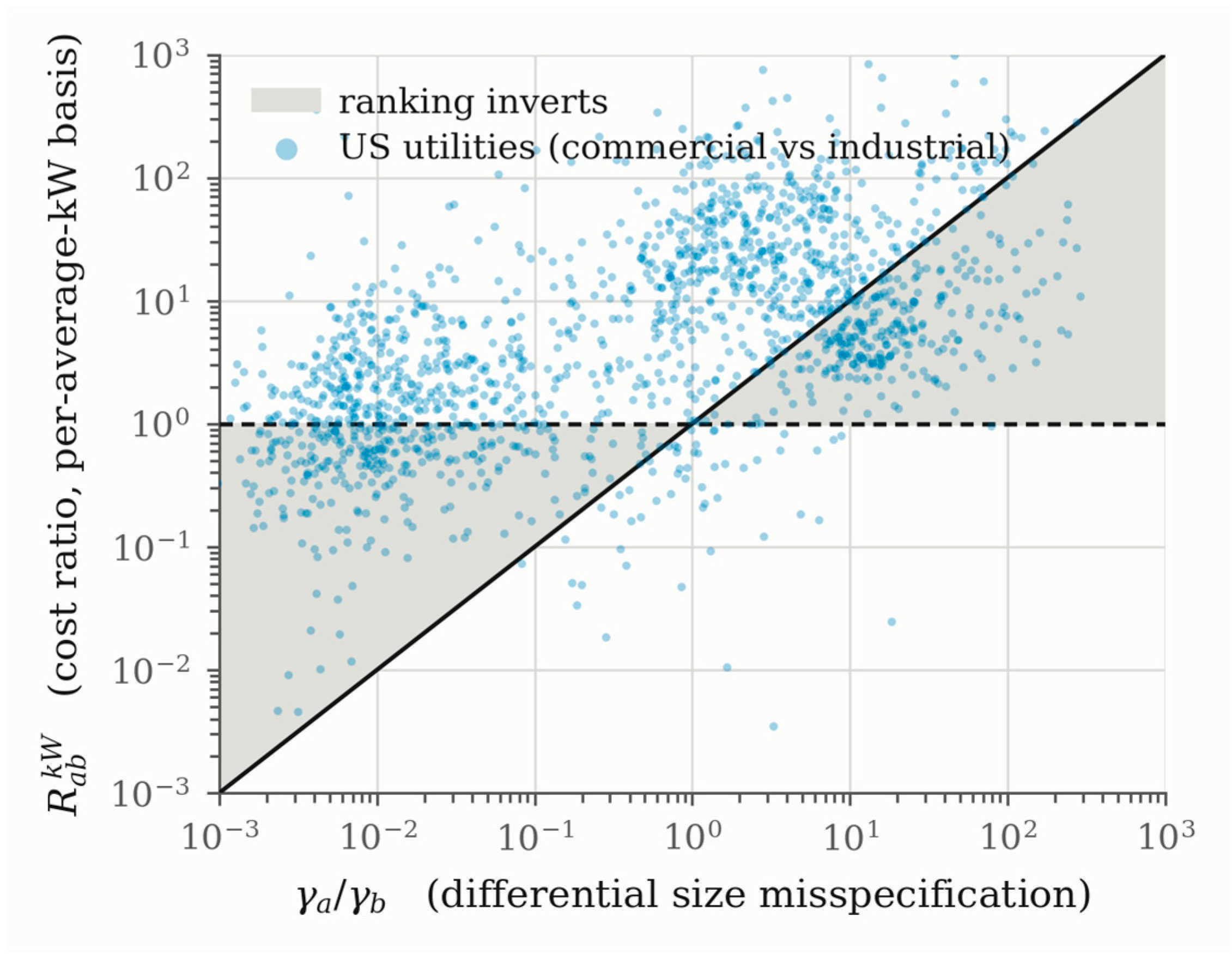
Figure 3.
Outage cost on both published bases for two customers whose annual use differs by only 2 kWh/yr. The two customers sit on opposite sides of the 50,000 kWh/yr class boundary. (a) On the per-event basis, moving the customer into the larger class raises its outage cost by a factor of 24.2 on average. (b) On the per-kilowatt basis, the same move lowers the cost by a factor of 15.3 on average. The two published bases therefore move the cost in opposite directions, and no choice of inflation adjustment, region, or duration can bring them into agreement.
Figure 3.
Outage cost on both published bases for two customers whose annual use differs by only 2 kWh/yr. The two customers sit on opposite sides of the 50,000 kWh/yr class boundary. (a) On the per-event basis, moving the customer into the larger class raises its outage cost by a factor of 24.2 on average. (b) On the per-kilowatt basis, the same move lowers the cost by a factor of 15.3 on average. The two published bases therefore move the cost in opposite directions, and no choice of inflation adjustment, region, or duration can bring them into agreement.
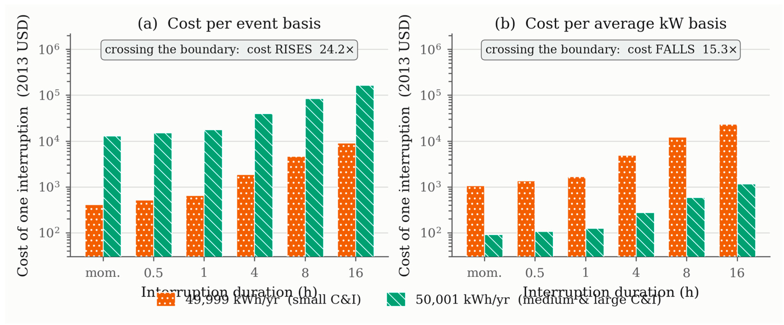
Figure 4.
Size mismatch factor γc across 2,060 U.S. utilities (Form EIA-861, 2014). The dashed line at γ = 1 marks where the per-event basis is exact. The shaded band marks a factor of two on either side. Residential values cluster tightly near one, while commercial values form two peaks and industrial values are skewed to the left. The two commercial peaks are the two sides of the 50,000 kWh/yr class boundary. The gap between them spans more than two orders of magnitude in γ.
Figure 4.
Size mismatch factor γc across 2,060 U.S. utilities (Form EIA-861, 2014). The dashed line at γ = 1 marks where the per-event basis is exact. The shaded band marks a factor of two on either side. Residential values cluster tightly near one, while commercial values form two peaks and industrial values are skewed to the left. The two commercial peaks are the two sides of the 50,000 kWh/yr class boundary. The gap between them spans more than two orders of magnitude in γ.
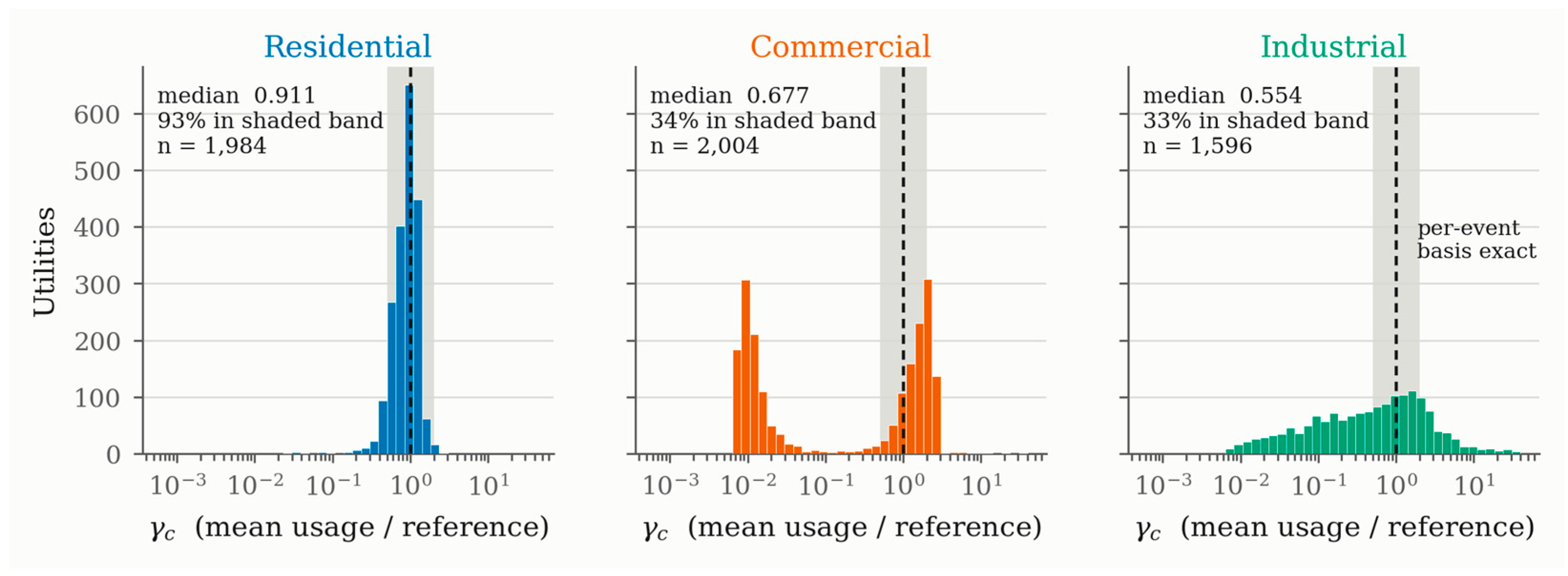
Figure 5.
Effect of the basis choice across 1,989 U.S. utilities for a four-hour outage. (a) Ratio of total zone cost on the two bases. The box in (a) gives the share of utilities at which the per-event total is higher (67%). It also gives the median (4.91) and the 90th percentile (about 80) of this ratio across utilities. The values fall on both sides of one, so the per-event basis overstates the total for some utilities and understates it for others. (b) Number of utilities at which the class with the largest cost share changes, grouped by the direction of the change. Reversals run both ways, so no single correction factor can remove them.
Figure 5.
Effect of the basis choice across 1,989 U.S. utilities for a four-hour outage. (a) Ratio of total zone cost on the two bases. The box in (a) gives the share of utilities at which the per-event total is higher (67%). It also gives the median (4.91) and the 90th percentile (about 80) of this ratio across utilities. The values fall on both sides of one, so the per-event basis overstates the total for some utilities and understates it for others. (b) Number of utilities at which the class with the largest cost share changes, grouped by the direction of the change. Reversals run both ways, so no single correction factor can remove them.
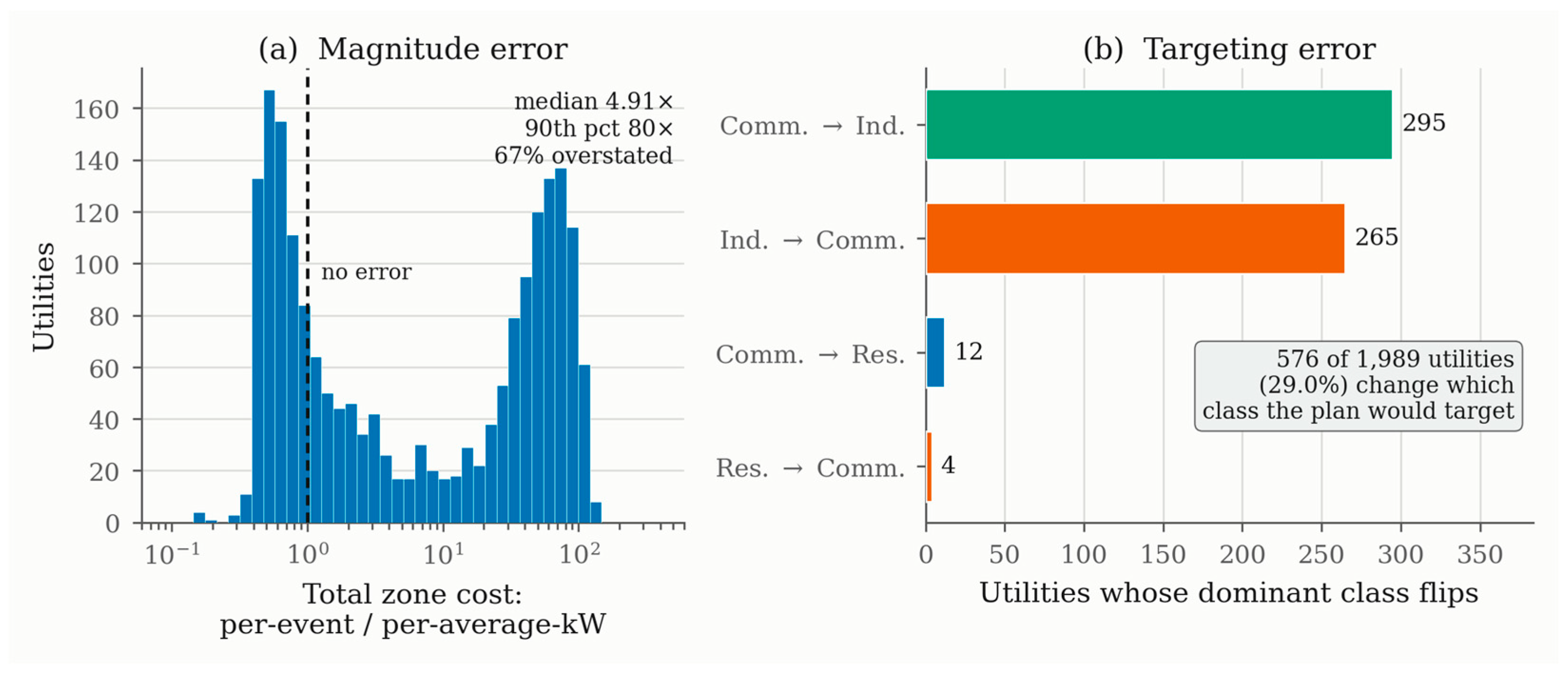
Figure 6.
Four-hour outage of the substation with three feeders. (a) Share of outage cost by class on each basis. On the per-event basis, medium and large C&I customers appear to carry 91.7% of the cost. On the per-kilowatt basis, small C&I customers carry 78.2%. The two bases therefore point to different hardening work. (b) Total cost on each basis at a load factor of 0.55.
Figure 6.
Four-hour outage of the substation with three feeders. (a) Share of outage cost by class on each basis. On the per-event basis, medium and large C&I customers appear to carry 91.7% of the cost. On the per-kilowatt basis, small C&I customers carry 78.2%. The two bases therefore point to different hardening work. (b) Total cost on each basis at a load factor of 0.55.
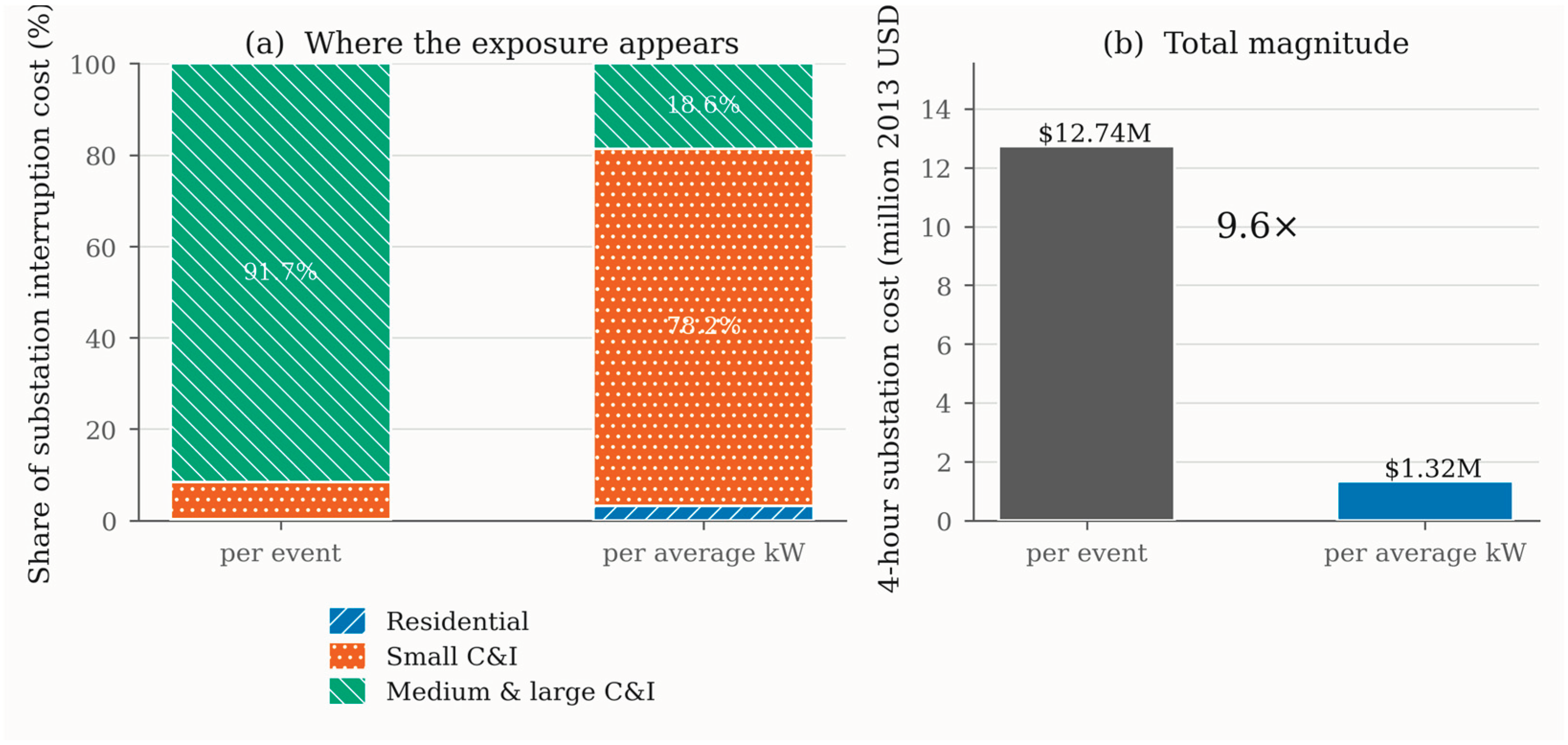

Table 1.
Check of Proposition 1 against the published tables. Implied demand is averaged over the six durations in the tables, and reference demand is .
Table 1.
Check of Proposition 1 against the published tables. Implied demand is averaged over the six durations in the tables, and reference demand is .
| Class | (GWh/yr) | Implied (kW) | Reference (kW) | Ratio | CV (%) |
|---|---|---|---|---|---|
| Residential | 0.0134 | 1.5300 | 1.5241 | 1.004 | 1.20 |
| Small C&I | 0.0192 | 2.1934 | 2.1934 | 1.000 | 0.02 |
| Medium & large C&I | 7.1405 | 815.2505 | 815.1257 | 1.000 | 0.09 |
Table 2.
Effect of the cost basis across 1,989 U.S. utilities for a four-hour outage.
| Quantity | Value |
|---|---|
| Utilities analyzed | 1,989 |
| Utilities where the leading class changes | 576 |
| as a share of utilities (%) | 29.0 |
| commercial → industrial | 295 |
| industrial → commercial | 265 |
| commercial → residential | 12 |
| residential → commercial | 4 |
| Ratio of per-event to per-kW total cost, median | 4.91 |
| 10th percentile | 0.50 |
| 90th percentile | 79.65 |
| Utilities where the per-event total is higher (%) | 66.8 |
Table 3.
Four-hour outage of the whole substation on both bases. The cost shares do not change with the load factor. Only the size of the per-kilowatt total depends on it.
Table 3.
Four-hour outage of the whole substation on both bases. The cost shares do not change with the load factor. Only the size of the per-kilowatt total depends on it.
| Class | nc | Mean (kW) | γc | per ev. (%) | per kW (%) |
|---|---|---|---|---|---|
| Residential | 3,323 | 3.67 | 1.3240 | 0.2 | 3.1 |
| Small C&I | 549 | 4.00 | 1.0030 | 8.1 | 78.2 |
| Medium & large C&I | 296 | 31.26 | 0.0211 | 91.7 | 18.6 |
Table 4.
Substation totals at two load factors. The class with the largest cost share stays the same, and only the size of the totals changes.
Table 4.
Substation totals at two load factors. The class with the largest cost share stays the same, and only the size of the totals changes.
| Load factor | Per event (M$) | Per kW (M$) | Ratio |
|---|---|---|---|
| 0.55 | 12.74 | 1.32 | 9.63 |
| 1.00 | 12.74 | 2.41 | 5.30 |
Disclaimer/Publisher’s Note: The statements, opinions and data contained in all publications are solely those of the individual author(s) and contributor(s) and not of MDPI and/or the editor(s). MDPI and/or the editor(s) disclaim responsibility for any injury to people or property resulting from any ideas, methods, instructions or products referred to in the content. |
© 2026 by the authors. Licensee MDPI, Basel, Switzerland. This article is an open access article distributed under the terms and conditions of the Creative Commons Attribution (CC BY) license (http://creativecommons.org/licenses/by/4.0/).
Copyright: This open access article is published under a Creative Commons CC BY 4.0 license, which permit the free download, distribution, and reuse, provided that the author and preprint are cited in any reuse.