

Submitted:
25 October 2026
Posted:
28 October 2026
You are already at the latest version
Preprints on COVID-19 and SARS-CoV-2
Abstract
The pandemic significantly disrupted Global Financial Markets, which had never experienced such unusual levels of volatility and uncertainty since the Covid-19 outbreak. The post-recovery phase saw continued price fluctuations due to inflation, geopolitical conflicts, and economic policy changes.This study examines the volatility and market behaviour of six major global stock market indices — S&P 500, FTSE 100, DAX, Nikkei 225, NIFTY 50, and Shanghai Composite — using daily data from January 2019 to April 2026. The data is divided into three sub-periods: pre-COVID (2019), COVID (2020), and post-COVID (2021–2026). A combination of statistical, econometric, clustering, and machine learning methods is applied, including descriptive statistics, correlation analysis, ADF test, ARCH LM test, GARCH (1,1), K-Means clustering, PCA, Random Forest, XGBoost, and Support Vector Regression (SVR) with an RBF kernel. The GARCH (1,1) model confirmed high volatility persistence across all markets. Among the machine learning models, Random Forest achieved the best overall prediction performance with a mean R² of 0.7678, mean RMSE of 0.003384, and mean MAE of 0.001973, followed by XGBoost (R²=0.7565) and SVR (R²=0.5851). The findings indicate that the COVID-19 pandemic was associated with persistent changes in global stock market volatility and behaviour that extended into the post-COVID period.
Keywords:
stock market volatility
; COVID-19
; GARCH model
; machine learning
; random forest
; XGBoost
; SVR
; leading global stock markets
; post-COVID analysis
1. Introduction
Stock markets worldwide form the backbone of the global economy. They help create capital and allow investors to invest their money. Macroeconomic factors, such as inflation, interest rates, government policies, and significant global events, directly affect the performance of the stock market. The markets of all the countries of the world are interconnected due to increasing financial globalization, so whatever happens or occurs in one country can affect other countries too.
The COVID-19 pandemic brought about the most severe disturbance to the world’s financial markets. There were sudden decreases in prices, panic selling, and chaotic fluctuations within the market during the pandemic. The lockdowns, disruptions in the supply chains, and the economic uncertainty negatively affected investors and businesses worldwide. The market began to recover from the initial effects of the pandemic, but the changes made by COVID-19 have continued to persist due to the increase in the level of inflation and the existence of different policy situations and geopolitical issues.
While previous studies have documented the immediate impact of COVID-19 on stock markets (Ashraf 2020; Baek et al., 2020; Zhang et al., 2020), fewer studies have analyzed long-term post-pandemic behaviour using a combined statistical, econometric, and machine learning framework covering data through 2026. This study addresses that gap by examining volatility and market behaviour of six major global indices across three periods using GARCH modelling, clustering analysis, and non-linear machine learning models including SVR with an RBF kernel — which is theoretically motivated by the confirmed non-linear heteroscedastic nature of financial volatility.
The COVID-19 pandemic has created one of the biggest disruptions in financial market history over the last ~30 years. For example, during the pandemic, there were suddenly sharp price drops overall for most stocks; there was panic selling; and there was extremely high volatility (upside-down movement) in overall equity markets, due to lockdowns around the world; supply chains collapsing; and uncertainty regarding how the world economy would react to everything. While the markets recovered somewhat after the initial shock, the impacts of COVID-19 continued with the inflation that we are currently facing, current geopolitical conflicts, and the new policies that governments are creating as a result of the pandemic.
A significant focus of research in finance and economics has historically been placed on financial market volatility due to the critical implications of volatility for portfolio management, risk assessment, asset pricing, and investment choices. The development of econometric models that can capture evolving volatility patterns has had a substantial impact on our understanding of how financial markets behave. The theoretical foundation for volatility modelling was established by (Engle, 1982) with the ARCH model and extended by (Bollerslev, 1986) with GARCH, which became the standard tool for financial volatility analysis. These two initial models are considered the fundamental building blocks for all future work in financial econometrics because they can capture "volatility clustering," a common feature of stock market returns. (Nelson, 1991) proposed using alternative volatility specifications that can model asymmetric market responses to shocks. Whereas (Ding, Granger, and Engle, 1993) identified long-memory characteristics in financial volatility. The theoretical and practical use of volatility modeling has been thoroughly evaluated by (Brooks, 2019), (Tsay, 2010), (Gujarati and Porter, 2009), and (Wooldridge, 2016). These authors emphasize that volatility analysis must be used because it provides crucial insight for apprehending the dynamics and risks related to financial markets.
(Ashraf, 2020) found that increasing COVID-19 cases negatively affected stock market returns globally. (Baek, Mohanty, and Glambosky, 2020) documented a sharp increase in market volatility during the pandemic. (Zhang, Hu, and Ji, 2020) found global markets to be highly uncertain. (Harjoto, Rossi, and Paglia, 2021) found that markets reacted strongly to pandemic-related news and government stimulus. (Bissoondoyal-Bheenick et al., 2021) found that stock return and volatility connectedness increased as the COVID-19 pandemic intensified. (Vo, Vo, and Nguyen, 2022) also found that the level of volatility increased while the connections between markets were stronger throughout the pandemic period.
Machine learning techniques are playing an ever-increasing role in the search for new ways to predict financial returns. (Fischer and Krauss, 2018) found that deep learning models perform better than traditional approaches to predict financial returns. The introduction of XGBoost, by (Chen and Guestrin, 2016) has led to strong results on many predictive tasks. The introduction of SVR, by (Drucker, Burges, Kaufman, Smola, and Vapnik, 1997) has provided a method that uses kernel functions to model non-linear relationships. The present study combines GARCH-based volatility modeling with three non-linear machine learning models — Random Forest, XGBoost, and SVR with RBF kernel — applied to post-COVID stock market data through April 2026.
1.2. Theoretical Framework
This study is based on the theories of Efficient Markets (EMH), volatility clustering, market links and epidemic influences, & the chaotic nature of market rates of return. Thus, these theoretical viewpoints give a combined basis of knowledge regarding the effects that a major worldwide shock, & the COVID-19 pandemic represents one, may have on the volatility of stock markets, volatility, and persistence. Also, it will affect international market synchronization & the prediction of volatility.
Efficient Market Hypothesis and Information Uncertainty
(Fama, 1970) developed the Efficient Market Hypothesis (EMH), which offers basic theoretical background for explaining market price movements. EMH states that share prices will reflect all existing information and that an immediate response to new information will be given. However, the COVID-19 Pandemic created a unique information situation filled with uncertainty about the number of infected individuals, the government's response through lockdowns and economic regulations, the government's financial response, the Federal Reserve's financial policies, and the eventual economic recovery. Such an environment can generate substantial changes in investor expectations and consequently influence asset prices and market volatility. Therefore, the COVID-19 pandemic provides an important setting for examining how an extreme information shock affects the behaviour of international stock markets.
Volatility Clustering and Persistence
Financial markets are known for their characteristic volatility clusters. This means that periods of high volatility are followed by other highly volatile periods, whereas periods of low or no volatility are followed by other low or no volatile periods. An established theoretical basis for the time-varying behaviour of risk in the financial market can be found in ARCH and GARCH frameworks.For the purpose of current research, this point of view is important, as an impactful event such as the pandemic can have lasting effects that occur after the initial shock to financial markets has occurred. Thus, if the pandemic resulted in continued volatility and disrupted normal trading patterns, then that volatility should still be evident throughout the subsequent recovery phase. For that reason, this paper will research ARCH- and GARCH-based volatility persistence for pre-COVID-19, COVID-19, and post-COVID-19 periods.
Market Interconnectedness and Crisis Synchronization
Financial globalization has increased the level of integration in international financial markets. Therefore, a shock occurring in one market could be transmitted to other markets via informational channels, investor actions, international capital flows, and the presence of shared sources of uncertainty.
During periods of financial stress, international markets may become more synchronized because investors respond to similar global information and uncertainty. The COVID-19 pandemic represents an important example of such a common global shock. Thus, changes in correlations among the selected stock markets provide an important perspective for understanding whether the International Stock Market synchronised during the crisis and whether it returned back to pre-Pandemic levels after the Crisis as well.
Nonlinear Behaviour and Volatility Predictability
There are many times when financial returns will show non-normality (long tails) and volatility clustering (periods of extreme price fluctuation tied closer together) along with a nonlinear relationship (dependence not based on a straight line). Because of this, it can be argued that linear approximations are often not sufficient when trying to model the way a financial market will behave.
The purpose of this theoretical point of view brings to light the importance of using machine learning in this research project. The three machine learning techniques used in this project (Random Forest, XGBoost, and Support Vector Regression) can model the relationship between past market features and future volatility that represents a nonlinear relationship. Thus, this is not just an additional method of statistical analysis but also a theory based on nonlinear characteristics of financial market volatility.
1.3. Research Gap
While the impact of COVID-19 on financial markets has been thoroughly studied and documented in a wide range of literature and journal articles, much remains to be learned concerning the long-run characteristics and behaviour of the global stock markets subsequent to a large-scale financial crisis. The most popular recent studies of this type of event concentrated largely on the immediate impact that the pandemic had on all aspects of the stock market (e.g., returns, volatility, uncertainty, and contiguity between individual equities). Little has been discussed, however, on how the event continued to affect the stock market during the recovery phase after the pandemic occurred and whether the characteristics of stock market volatility were different from what they had been before the pandemic.
Firstly, there exists an incomplete understanding of how crisis-driven volatility continues to exist. The fact that volatility will be high during a crisis does not guarantee that volatility will remain high continuously even after the crisis has ended. It is important to differentiate between what I will call temporary responses to a shock in the market and enduring levels of volatility after the initial period of the shock has subsided. Thus, analysis of the pre-COVID, COVID, and post-COVID timelines in the financial markets will provide relevant and useful insights for understanding whether the influence of the pandemic continued to shape the risk behaviour of financial instruments during the recovery phase.
Second, there is a gap concerning international market synchronization. The COVID-19 pandemic represented a common global shock that affected developed and emerging economies simultaneously. Such a common shock may increase synchronization among international stock markets as investors respond to similar information, uncertainty, and global economic conditions. While previous research has documented increased market co-movement during periods of financial stress, there remains a need to examine whether this increased synchronization persisted or declined during the post-COVID period.
Third, there is a gap concerning the relationship between volatility dynamics and predictability. Financial returns exhibit characteristics such as volatility clustering, persistence, and nonlinear behaviour. These characteristics suggest that historical market information may contain useful information about subsequent volatility. However, volatility behaviour and volatility forecasting are often examined as separate issues. The present study connects these perspectives by examining volatility characteristics through econometric analysis and subsequently evaluating the predictive performance of nonlinear machine learning approaches.
The present study addresses these gaps by examining six major global stock market indices representing both developed and emerging economies across three periods: pre-COVID, COVID, and post-COVID. The study investigates volatility behaviour, volatility persistence, changes in market relationships, similarities in market behaviour, and the predictability of volatility using statistical, econometric, and machine learning approaches.
2. Theoretical Contribution
The theoretical contribution of the study lies in integrating several established perspectives of financial market behaviour into a unified post-crisis framework. Rather than treating volatility, market interconnectedness, and forecasting as independent empirical issues, the study conceptualizes them as interconnected dimensions of market adjustment following a major global shock.
The framework proposes that COVID-19-related information uncertainty influenced investor and market behaviour, leading to increased volatility and volatility persistence, while the common nature of the shock increased synchronization among international markets. The resulting volatility characteristics subsequently provided information relevant to volatility prediction.
Thus, the contribution of the study is primarily theoretical and integrative rather than mathematical. The study extends the understanding of post-COVID financial market behaviour by connecting information uncertainty, volatility clustering, persistence, international market synchronization, and nonlinear predictability within a single conceptual framework.
This perspective enables the study to move beyond simply documenting higher volatility during the COVID-19 period and instead examine how a major global shock influenced the persistence, interconnectedness, adjustment, and predictability of international stock market behaviour.
2.1. Motivation and Objectives of the Study
The COVID-19 pandemic generated unprecedented disruptions in global financial markets, resulting in extreme volatility, increased market uncertainty, and stronger interconnectedness among stock exchanges worldwide. Although numerous studies have examined the immediate impact of COVID-19 on financial markets, relatively limited research has focused on the long-term post-COVID behaviour of global stock market volatility. Understanding whether volatility patterns and market relationships returned to pre-pandemic conditions or continued to exhibit structural changes remains important for investors, policymakers, and financial analysts. Furthermore, the increasing application of machine learning techniques in financial forecasting creates an opportunity to compare traditional econometric models with modern predictive approaches in a unified analytical framework.
Therefore, the primary objectives of this study are: (i) to examine the volatility behaviour of six major global stock market indices during the pre-COVID, COVID, and post-COVID periods; (ii) to investigate volatility persistence using ARCH and GARCH models; (iii) to analyse changes in market interconnectedness and clustering patterns across different periods; (iv) to evaluate and compare the predictive performance of Random Forest, XGBoost, and Support Vector Regression (SVR) models for volatility forecasting; and (v) to assess whether the COVID-19 pandemic produced long-term structural changes in global stock market behaviour.
3. Data and Methodology
3.1. Data
Daily closing price data for six global stock market indices — S&P 500 (USA), FTSE 100 (UK), DAX (Germany), Nikkei 225 (Japan), NIFTY 50 (India), and Shanghai Composite (China) — were collected from Investing.com for January 2019 to April 2026. The study period is divided into: Pre-COVID (January 2019–December 2019), COVID (January 2020–December 2020), and Post-COVID (January 2021–April 2026).
3.2. Log Returns and Volatility
Daily log returns are calculated as Rₜ = ln(Pₜ/Pₜ₋₁). Rolling 21-day standard deviation annualized by √252 is used as the volatility measure for machine learning models.
3.3. Statistical and Econometric Methods
Descriptive statistics, correlation analysis, ADF stationarity test, ARCH LM test, and GARCH (1,1) with Student's t-distribution are applied. The GARCH model is: σ²ₜ = ω + αε²ₜ₋₁ + βσ²ₜ₋₁, where α+β measures overall volatility persistence.
3.4. Machine Learning Models
Random Forest, XGBoost, and SVR with an RBF kernel are used to predict next-day volatility. Features include lag values (1,2,3,5,10 days), 5-day and 10-day rolling mean, 5-day rolling standard deviation, and a period indicator. A chronological 80:20 train-test split is applied. SVR requires StandardScaler feature normalization before training. All models are evaluated using R², RMSE, and MAE.
4. Results
4.1. Descriptive Statistics
Table 1 presents descriptive statistics of daily returns. All indices show positive but near-zero mean returns, negative skewness, and kurtosis well above 3, confirming non-normality and fat-tailed distributions. This justifies the use of Student's t-distribution in GARCH estimation.
4.2. Price Trends and Rolling Volatility
Figure 1 shows the price trends of all six indices from 2019 to 2026 across the three sub-periods. All markets show a sharp decline during the COVID period (2020) followed by divergent recovery patterns in the post-COVID period.
Figure 2 presents the 30-day rolling volatility for all six global stock market indices. All markets experienced peak volatility during March–April 2020, reflecting the severe financial uncertainty associated with the COVID-19 pandemic. Although volatility gradually declined during the post-COVID period, it remained above pre-pandemic levels for several markets. Additional volatility spikes were observed during later periods, indicating that global financial markets continued to experience intermittent episodes of uncertainty and elevated risk even after the initial pandemic shock had subsided.
Table 2 presents the mean volatility of the six stock market indices across the pre-COVID, COVID, and post-COVID periods. The results show that COVID-19 was associated with a substantial increase in volatility across most markets. There was a relatively lower growth rate in Shanghai, likely because of earlier cases of confinement in China. After the pandemic, there was lesser volatility compared to prior levels for most indexes.
4.3. Correlation Analysis
Figure 3 shows the full-period correlation heatmap. The strongest relationship is between FTSE 100 and DAX (r = 0.822), reflecting European market integration. The weakest is between S&P 500 and Shanghai (r = 0.193).
Figure 4 shows that average pairwise correlation increased from 0.3253 (pre-COVID) to 0.5327 (COVID), confirming stronger market interconnectedness during the crisis, before declining to 0.3349 in the post-COVID period.
4.4. Stationarity and Autocorrelation Tests
Table 3 presents the ADF test results. All six-return series are stationary at the 5% level (p = 0.000 for all indices), confirming suitability for GARCH modelling.
The autocorrelation of returns for each index is shown in Figure 5. Autocorrelation drops off quickly and is nearly zero at the longest lags. This indicates that returns are not serially dependent, which is consistent with the results from the ADF test for stationarity. Conversely, Figure 6 shows the autocorrelation of the squared returns, and the autocorrelation of squared returns at most lags is significant. Significant autocorrelation exists at all lags. This demonstrates the existence of volatility clustering within a time series, which is a very typical condition in finance where there are long periods of high volatility followed by more periods of high volatility. This evidence provides a strong case for using GARCH models in the study of this phenomenon.
4.5. ARCH LM Test Results
Table 4 reports the ARCH-LM test results for the six global stock market indices over the full study period. The statistically significant results indicate the presence of conditional heteroscedasticity and provide empirical justification for applying GARCH-based volatility modelling.
All six indices exhibit significant ARCH effects (p < 0.001) over the full study period, confirming the presence of time-varying volatility in global stock market returns. Figure 7 presents the ARCH-LM test results across the three study periods. During the pre-COVID period, significant ARCH effects were observed only for the S&P 500 and Shanghai Composite Index, suggesting relatively limited volatility clustering in most markets. However, by the post-COVID period, all six indices displayed significant ARCH effects, indicating that volatility clustering became more widespread and persistent following the pandemic. These findings suggest that market shocks continued to influence future volatility even after the immediate effects of COVID-19 had subsided, thereby supporting the use of GARCH models for volatility analysis.
4.6. GARCH (1,1) Results
Table 5 presents the estimated GARCH (1,1) parameters for the six selected stock market indices. The estimates indicate substantial volatility persistence, with α + β values close to unity for most markets.
The estimated GARCH parameters indicate substantial volatility persistence across all six stock market indices. The α + β values are close to unity for all markets, suggesting that the effects of volatility shocks remain influential for extended periods and dissipate only gradually over time. Among the selected indices, the S&P 500 exhibits the highest volatility persistence (α + β = 0.9776), indicating that market disturbances have particularly long-lasting effects in the U.S. market. NIFTY 50 records the highest β coefficient (0.8712), implying that past volatility plays a dominant role in determining current volatility and that volatility episodes tend to persist once initiated. In contrast, FTSE 100 shows the highest α coefficient (0.1781), suggesting a stronger immediate response to new market information and external shocks. Overall, these findings confirm the presence of persistent volatility dynamics across both developed and emerging markets during the post-COVID period.
Table 6 compares volatility persistence (α + β) across the pre-COVID, COVID, post-COVID, and full-study periods. The results demonstrate exceptionally high persistence during the COVID period and continued persistence in several markets during the post-COVID period.
During the COVID period, the S&P 500, DAX, and NIFTY 50 recorded α + β values equal to 1.000, indicating an Integrated GARCH (IGARCH) condition. This suggests that volatility shocks exhibited extremely high persistence and their effects remained influential for prolonged periods, reflecting the exceptional uncertainty and market stress experienced during 2020. In the post-COVID period, volatility persistence declined across most indices, indicating a gradual stabilization of market conditions. However, persistence remained notably high for the S&P 500 (0.9678) and NIFTY 50 (0.9683), suggesting that the impact of market shocks continued to influence volatility dynamics well beyond the pandemic period.
Figure 8 presents the estimated GARCH (1,1) conditional volatility for the six selected global stock market indices over the full study period. The figure illustrates the pronounced volatility spikes during the COVID-19 period and the subsequent moderation of volatility during the post-COVID period.
Figure 9 provides a visual comparison of GARCH volatility persistence across the pre-COVID, COVID, post-COVID, and full-study periods. The figure highlights the exceptionally high persistence observed during the COVID period and the continued persistence in selected markets during the post-COVID period.
4.7. Clustering Analysis
K-Means clustering (k = 3) combined with PCA visualization reveals that the relationships among global stock markets changed considerably across the three study periods. Pre-COVID, S&P 500, DAX, FTSE 100, and Nikkei 225 demonstrated similar return and volatility profiles, which indicated similar market performance. During COVID, S&P 500, DAX, FTSE 100, and NIFTY 50 appeared in the same cluster, meaning that COVID put more of the major global markets together. In post-COVID times, S&P 500, DAX, NIFTY 50, and Shanghai Composite are in one cluster, and FTSE 100 and Nikkei 225 are much farther apart, which shows different ways they recovered. These results show that since COVID, the way the markets relate to each other has changed a lot, so people now think differently about how the markets are connected. Therefore, because of the limited number of indices studied (n = 6), this should be considered an "exploratory" study and NOT a definitive classification of the markets studied.
4.8. Random Forest Results
Table 7 presents the predictive performance of the Random Forest model for each of the six stock market indices. The results indicate strong predictive performance across the selected markets, with a mean R² of 0.7678.
Feature importance analysis identified current volatility level and 5-day rolling standard deviation as the most influential predictors. This finding is consistent with the presence of volatility clustering identified through the ARCH and GARCH analyses, where recent volatility patterns play a significant role in determining future volatility. The superior performance of Random Forest suggests that stock market volatility contains nonlinear relationships that are effectively captured by ensemble tree-based learning algorithms.
Figure 10 presents the K-Means clustering results using PCA visualization for the three study periods. The changing cluster composition illustrates differences in market behaviour and similarity across the pre-COVID, COVID, and post-COVID periods.
4.9. XGBoost Results
Table 8 reports the predictive performance of the XGBoost model across the six selected stock market indices. The model achieves a mean R² of 0.7565, indicating strong predictive capability across the sample.
XGBoost achieved strong predictive performance, with a mean R² of 0.7565, mean RMSE of 0.003867, and mean MAE of 0.002193. The highest predictive accuracy was observed for NIFTY 50 (R² = 0.8102), indicating that the model effectively captured volatility dynamics within the Indian market. Furthermore, XGBoost outperformed Random Forest for FTSE 100 and NIFTY 50, suggesting that the sequential boosting mechanism was better able to capture complex market-specific patterns in these indices. The overall performance of XGBoost demonstrates the effectiveness of boosting-based ensemble methods in modelling nonlinear relationships and volatility behaviour in financial time series data.
Figure 12 presents the actual and XGBoost-predicted volatility values across the selected markets. The figure provides a visual assessment of the model's ability to capture the observed movements in volatility.
4.10. SVR Results
Table 9 presents the predictive performance of the SVR model with an RBF kernel across the six markets. Although its overall performance is lower than that of Random Forest and XGBoost, the model demonstrates useful predictive capability in capturing nonlinear volatility patterns.
SVR with an RBF kernel achieved a mean R² of 0.5851, mean RMSE of 0.004680, and mean MAE of 0.002506. The highest predictive accuracy was observed for NIFTY 50 (R² = 0.6899), indicating relatively better performance in modelling volatility dynamics within the Indian market. Although the predictive performance of SVR was lower than that of the ensemble-based models, the method remains theoretically well-suited for financial volatility forecasting due to the confirmed nonlinear and heteroscedastic nature of the return series. The actual against anticipated graphs show that SVR captures the overall trend and non-linear basis of volatility changes, but does not capture large fluctuations in volatility very well. Our findings indicate that non-linear kernel-based models can do an excellent job at capturing essential volatility patterns, but that the ensemble learning method is the most accurate predictive model for the markets we have analysed.
Figure 13 compares the actual volatility with the volatility predicted by the Support Vector Regression (SVR) model for six major stock market indices: S&P 500, FTSE 100, DAX, Nikkei 225, NIFTY 50, and Shanghai. The blue solid line represents the actual volatility, while the red dashed line represents the SVR-predicted values. Overall, the SVR model follows the general movement and temporal pattern of volatility reasonably well, although its ability to reproduce sudden and extreme volatility spikes varies across markets.
4.11. Model Comparison
Table 10 presents the full model comparison across all three-evaluation metrics.
By all three evaluation criteria, Random Forest straddled the optimal predictive model, exhibiting the highest average R² (0.7678), the lowest average RMSE (0.003384), and the lowest average MAE(0.001973). The consistent dominance of Random Forest among the multiple evaluation metrics affords considerable evidence of predictive reliability beyond the dependence on R². XGBoost was able to match Random Forest, and was better than Random Forest in the case of FTSE 100 and NIFTY 50 in the case of R², thus demonstrating market-targeted capture of the non-linear patterns. Random Forest, however, achieved lower RMSE and MAE, thus more reliable and accurate predictions in the case of most indices. Although SVR was inferior in R², the theoretical rationale for its inclusion was strengthened because the volatility series exhibited confirmed non-linear and heteroscedastic behaviors. The lower performance of SVR is in agreement with earlier works that investigate the superiority of ensemble learning approaches over kernel-based methods when lagged and rolling statistical features serve as predictors. The lowest predictive accuracy in all models was the Shanghai Composite Index, reflecting its isolated market and weaker link to the other global markets investigated in the study.
5. Discussion
The result shows various significant perspectives regarding the long-term global stock market's behavior after the COVID-19 pandemic had occurred. The continued high volatility after COVID, which was validated by the persistence estimates of GARCH model (α + β > 0.90) and analysis of rolling volatility, implies that the pandemic led to significant and long-lasting changes in the global financial marketplace, which lasted far beyond the initial stage of recovery. This aligns with Khan et al (2024), who found that there was continued volatility in developed and developing economies during the Post-Pandemic Period.
IGARCH demonstrated during the pandemic (α + β = 1.000 for S&P 500, DAX, and NIFTY 50) reveals the extent and length of the pandemic shock on world financial markets. The average pairwise correlation increased from 0.3253 pre-pandemic to 0.5327 amid the pandemic, representing the crisis contagion effect noted by Li et al (2021) and demonstrating that global markets were experiencing greater synchronisation during times of heightened uncertainty. Following this period, the average pairwise correlation declined to 0.3349 post-pandemic which reflects a partial restoration of market independence, though markets continue to remain highly interconnected compared to some pre-pandemic periods.
The outcome of machine learning has shown that past volatilities can be used to develop statistical features of the past as inputs in predicting future stock market volatility with reasonable accuracy. The superior result of Tree-Based methods (Random Forest and XGBoost) compared to SVR shows that Tree-Based methods are better in detecting complex relationships and nonlinear patterns in financial volatility datasets. The result is supported by the literature that has been growing rapidly on the usage of Ensemble Learning methods in financial forecasting and predicting volatility.
6. Limitations
This study focused on six major global stock market indices representing both developed and emerging economies. While these indices provide a broad representation of global market behaviour, the findings may not fully generalize to all international stock markets. Furthermore, the analysis primarily examined market volatility using historical price-based variables and did not incorporate macroeconomic indicators or sentiment-based measures. Future research may extend the analysis by including additional markets and explanatory variables to provide a more comprehensive understanding of post-COVID market dynamics.
7. Conclusion
The purpose of this study was to analyze the volatility and movement of prices for six major stock market indices worldwide between Jan 2019 – Apr 2026 using statistical, econometric, and machine learning tools. During the pandemic period, COVID-19 caused a massive and sudden increase in all market's volatility, which remained at much higher levels after the pandemic ended. The degree of correlation between international market indices increased substantially during the pandemic, but declined somewhat after the pandemic period ended. GARCH (1,1) results indicated that the global market continues to demonstrate high levels of volatility persistence, with the two markets, S&P 500 and NIFTY 50, demonstrating the greatest levels of volatility persistence after the end of the pandemic.Random Forest outperformed the other two machine learning models in predictive performance with mean R² value of 0.7678, a mean RMSE of 0.003384, and mean MAE of 0.001973 and also demonstrated a consistent advantage over all the other metrics used in the evaluation process. The XGBoost produced similar results; however, the SVR model with the RBF kernel, which was theoretically justified as a non-linear prediction model due to the verified presence of heteroscedasticity in the data set, yielded a mean R² value of 0.5851 as an overall indication of model predictive capability. The prediction accuracy of all models was the lowest in the case of the Shanghai Composite Index because of its unique market behavior during the overall observation period.
The study's overall findings show that the COVID-19 pandemic had lasting and significant effects on global equity market volatility that continued far into the post-COVID initial recovery period. The results will help investors, portfolio managers, and policymakers identify and understand the risks associated with investing in equity markets after the COVID-19 pandemic and create better-informed investment and risk management strategies.
Author Contributions
Conceptualization, B.S.M. and Z.H.S.; methodology, B.S.M. and Z.H.S.; software, Y.V. and J.R.M.; validation, B.S.M., Z.H.S. and S.B.; formal analysis, Y.V. and J.R.M.; investigation, B.S.M., Z.H.S. and M.M.S.; data curation, Y.V. and J.R.M.; writing—original draft preparation, B.S.M., Z.H.S., Y.V., M.M.S., S.B. and J.R.M.; writing—review and editing, B.S.M., Z.H.S., Y.V., M.M.S., S.B. and J.R.M.; visualization, Y.V. and J.R.M.; supervision, Z.H.S. and S.B.; funding acquisition, Z.H.S. All authors have read and agreed to the submitted version of the manuscript.
Funding
This research was funded by Kingdom University, grant number KU-2025-26-02”. .
Institutional Review Board Statement
Institutional Review Board Statement: Not applicable. This study used publicly available financial market data and did not involve human participants or animals.
Informed Consent Statement
This study used publicly available financial market data and did not involve human participants or animals.
Data Availability Statement
The authors acknowledge the data collected from www.investing.com. which is publicly available.
Acknowledgments
No additional acknowledgments to report.
Conflicts of Interest
The authors declare that they have no known competing financial interests or personal relationships that have influenced the work reported in this paper.
References
- Al-Awadhi, A. M.; Alsaifi, K.; Al-Awadhi, A.; Alhammadi, S. Death and Contagious Infectious Diseases: Impact of the COVID-19 Virus on Stock Market Returns. J. Behav. Exp. Financ. 2020, 27, 100326. [Google Scholar] [CrossRef] [PubMed]
- Ashraf, B. N. Stock Markets’ Reaction to COVID-19: Cases or Fatalities? Res. Int. Bus. Financ. 2020, 54, 101249. [Google Scholar] [CrossRef] [PubMed]
- Baek, S.; Mohanty, S. K.; Glambosky, M. COVID-19 and Stock Market Volatility: An Industry-Level Analysis. Financ. Res. Lett. 2020, 37, 101748. [Google Scholar] [CrossRef] [PubMed]
- Baker, S. R.; Bloom, N.; Davis, S. J.; Kost, K.; Sammon, M.; Viratyosin, T. The Unprecedented Stock Market Reaction to COVID-19. Rev. Asset Pricing Stud. 2020, 10(4), 742–758. [Google Scholar] [CrossRef]
- Bollerslev, T. Generalized Autoregressive Conditional Heteroskedasticity. J. Econom. 1986, 31(3), 307–327. [Google Scholar] [CrossRef]
- Breiman, L. Random Forests. Mach. Learn. 2001, 45(1), 5–32. [Google Scholar] [CrossRef]
- Caporin, M.; McAleer, M. Do We Really Need Both BEKK and DCC? A Tale of Two Multivariate GARCH Models. J. Econ. Surv. 2012, 26(4), 736–751. [Google Scholar] [CrossRef]
- Chen, T.; Guestrin, C. XGBoost: A Scalable Tree Boosting System. In Proceedings of the 22nd ACM SIGKDD International Conference on Knowledge Discovery and Data Mining, 2016; pp. 785–794. [Google Scholar] [CrossRef]
- Cont, R. Empirical Properties of Asset Returns: Stylized Facts and Statistical Issues. Quant. Financ. 2001, 1(2), 223–236. [Google Scholar] [CrossRef]
- Ding, Z.; Granger, C. W. J.; Engle, R. F. A Long Memory Property of Stock Market Returns and a New Model. J. Empir. Financ. 1993, 1(1), 83–106. [Google Scholar] [CrossRef]
- Drucker, H.; Burges, C. J. C.; Kaufman, L.; Smola, A. J.; Vapnik, V. Support Vector Regression Machines. Adv. Neural Inf. Process. Syst. 9 1997, 155–161. [Google Scholar]
- Engle, R. F. Autoregressive Conditional Heteroskedasticity with Estimates of the Variance of United Kingdom Inflation. Econometrica 1982, 50(4), 987–1007. [Google Scholar] [CrossRef]
- Fama, E. F. Efficient Capital Markets: A Review of Theory and Empirical Work. J. Financ. 1970, 25(2), 383–417. [Google Scholar] [CrossRef]
- Fischer, T.; Krauss, C. Deep Learning with Long Short-Term Memory Networks for Financial Market Predictions. Eur. J. Oper. Res. 2018, 270(2), 654–669. [Google Scholar] [CrossRef]
- Goodell, J. W. COVID-19 and Finance: Agendas for Future Research. Financ. Res. Lett. 2020, 35, 101512. [Google Scholar] [CrossRef] [PubMed]
- Harjoto, M. A.; Rossi, F.; Paglia, J. K. COVID-19: Stock Market Reactions to the Shock and the Stimulus. Appl. Econ. Lett. 2021, 28(10), 795–801. [Google Scholar] [CrossRef]
- Investing.com. Historical Stock Market Index Data. 2026. Available online: https://www.investing.com.
- Krauss, C.; Do, X. A.; Huck, N. Deep Neural Networks, Gradient-Boosted Trees, Random Forests: Statistical Arbitrage on the S&P 500. Eur. J. Oper. Res. 2017, 259(2), 689–702. [Google Scholar] [CrossRef]
- Bissoondoyal-Bheenick, Emawtee; Do, Hung; Hu, Xiaolu; Zhong, Angel. Learning from SARS: Return and Volatility Connectedness in COVID-19. Financ. Res. Lett. 2021, 41, 101796. [Google Scholar] [CrossRef] [PubMed]
- Malkiel, B. G. The Efficient Market Hypothesis and Its Critics. J. Econ. Perspect. 2003, 17(1), 59–82. [Google Scholar] [CrossRef]
- Narayan, P. K. COVID-19 Research Outcomes: An Agenda for Future Research. Econ. Anal. Policy 2021, 71, 439–445. [Google Scholar] [CrossRef]
- Nelson, D. B. Conditional Heteroskedasticity in Asset Returns: A New Approach. Econometrica 1991, 59(2), 347–370. [Google Scholar] [CrossRef]
- Schwert, G. W. Why Does Stock Market Volatility Change over Time? J. Financ. 1989, 44(5), 1115–1153. [Google Scholar] [CrossRef]
- Vo, X. V.; Vo, D. H.; Nguyen, T. C. COVID-19 and Stock Market Volatility: Evidence from Global Markets. Heliyon 2022, 8(2), e08806. [Google Scholar] [CrossRef] [PubMed]
- Zhang, D.; Hu, M.; Ji, Q. Financial Markets under the Global Pandemic of COVID-19. Financ. Res. Lett. 2020, 36, 101528. [Google Scholar] [CrossRef] [PubMed]
Figure 1.
Global Stock Market Price Trends (2019–2026). Green = Pre-COVID, Red = COVID, Blue = post-COVID.
Figure 1.
Global Stock Market Price Trends (2019–2026). Green = Pre-COVID, Red = COVID, Blue = post-COVID.
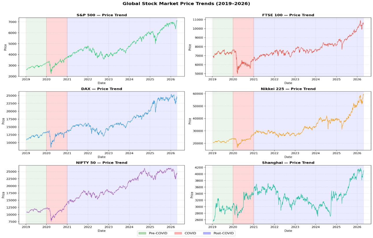
Figure 2.
30-Day Rolling Volatility — All Global Indices (2019–2026).
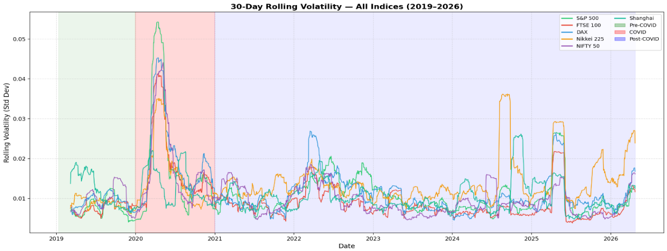
Figure 3.
Return Correlation Matrix Heatmap — Full Period (2019–2026).
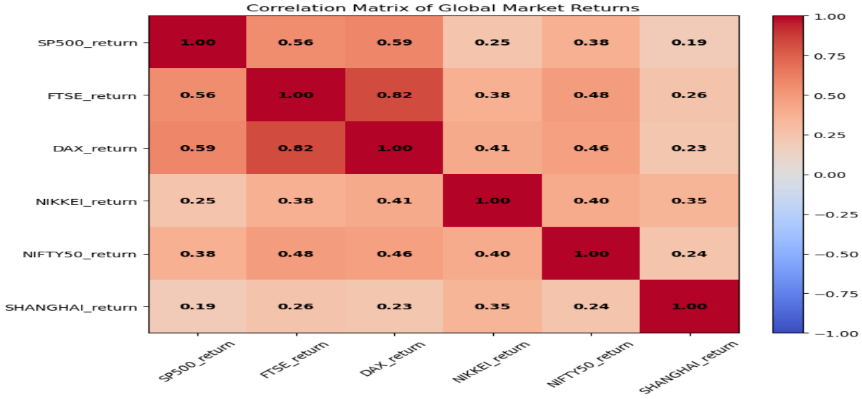
Figure 4.
Average Pairwise Correlation by Period.
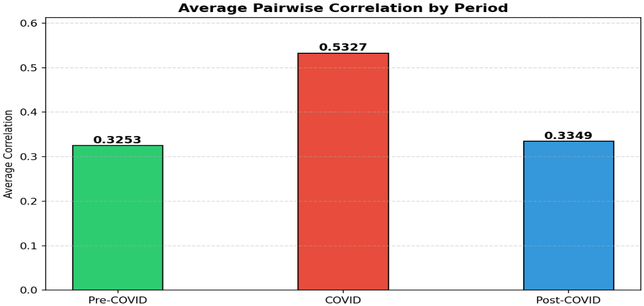
Figure 5.
Autocorrelation Function (ACF) of Returns — All Global Indices.
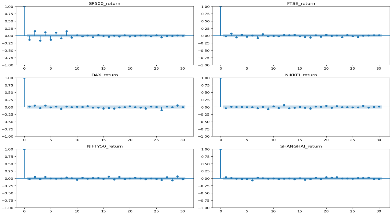
Figure 6.
Autocorrelation Function (ACF) of Squared Returns — All Global Indices.
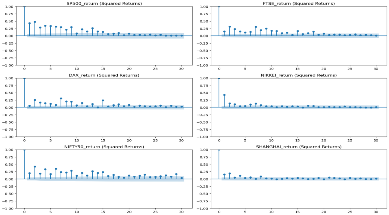
Figure 7.
ARCH Test p-values by Period — All Global Indices. Green = ARCH effects present (p < 0.05).
Figure 7.
ARCH Test p-values by Period — All Global Indices. Green = ARCH effects present (p < 0.05).
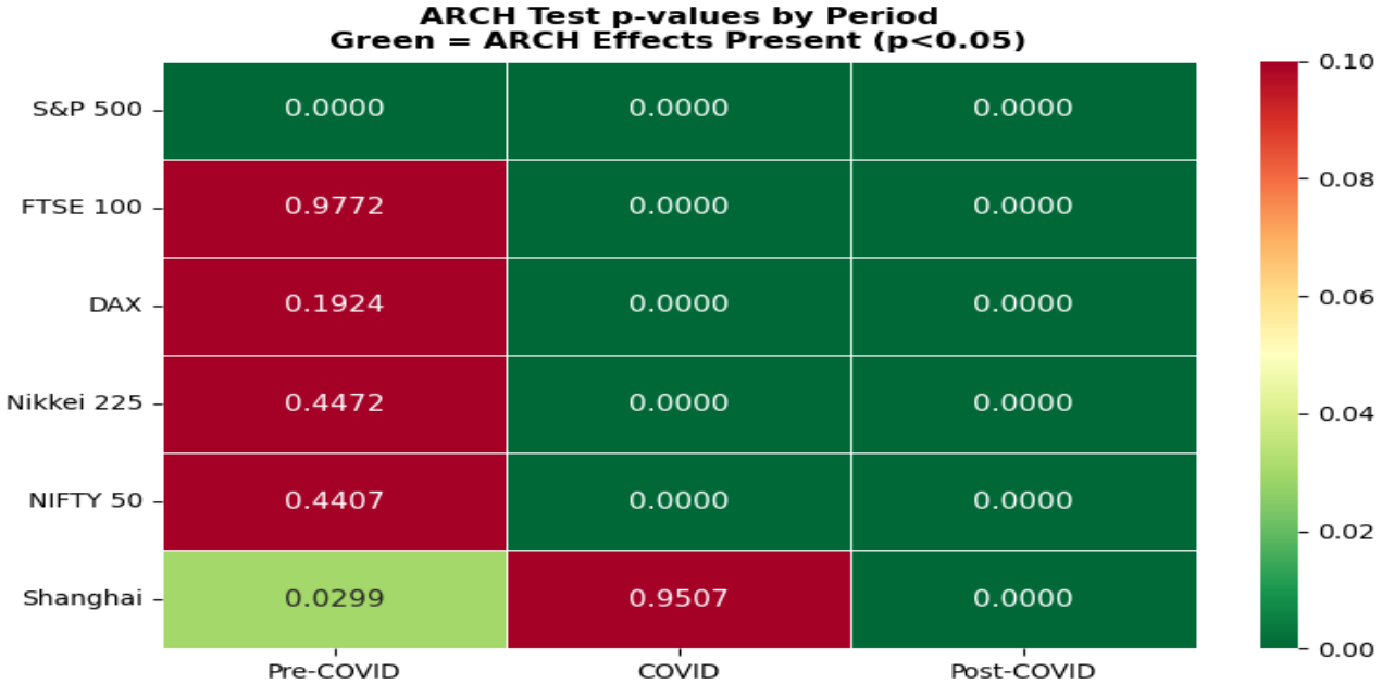
Figure 8.
GARCH (1,1) Conditional Volatility — Global Indices (2019–2026).
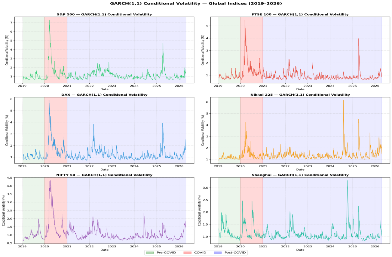
Figure 9.
GARCH (1,1) Volatility Persistence (α+β) by Period — All Indices.
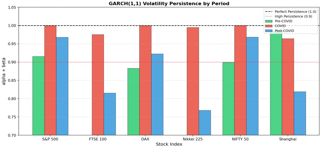
Figure 10.
K-Means Clustering — Global Stock Indices by Period (PCA Visualization). PC1 and PC2 explain 52–54% and 29–31% of variance, respectively across sub-periods.
Figure 10.
K-Means Clustering — Global Stock Indices by Period (PCA Visualization). PC1 and PC2 explain 52–54% and 29–31% of variance, respectively across sub-periods.
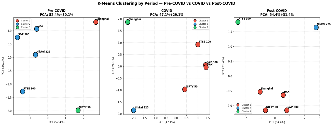
Figure 11.
Random Forest — Actual vs Predicted Volatility (All Indices).
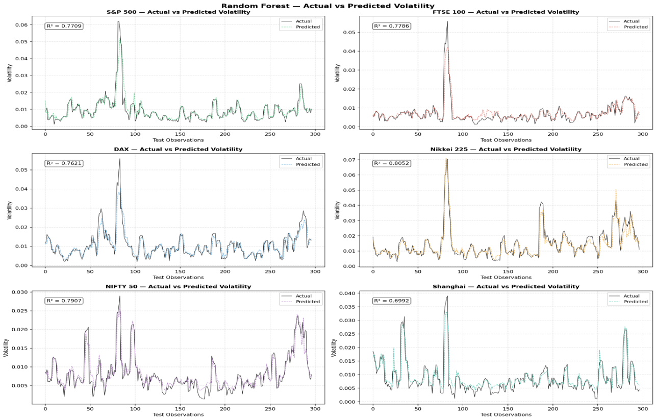
Figure 12.
XGBoost — Actual vs Predicted Volatility (All Indices).
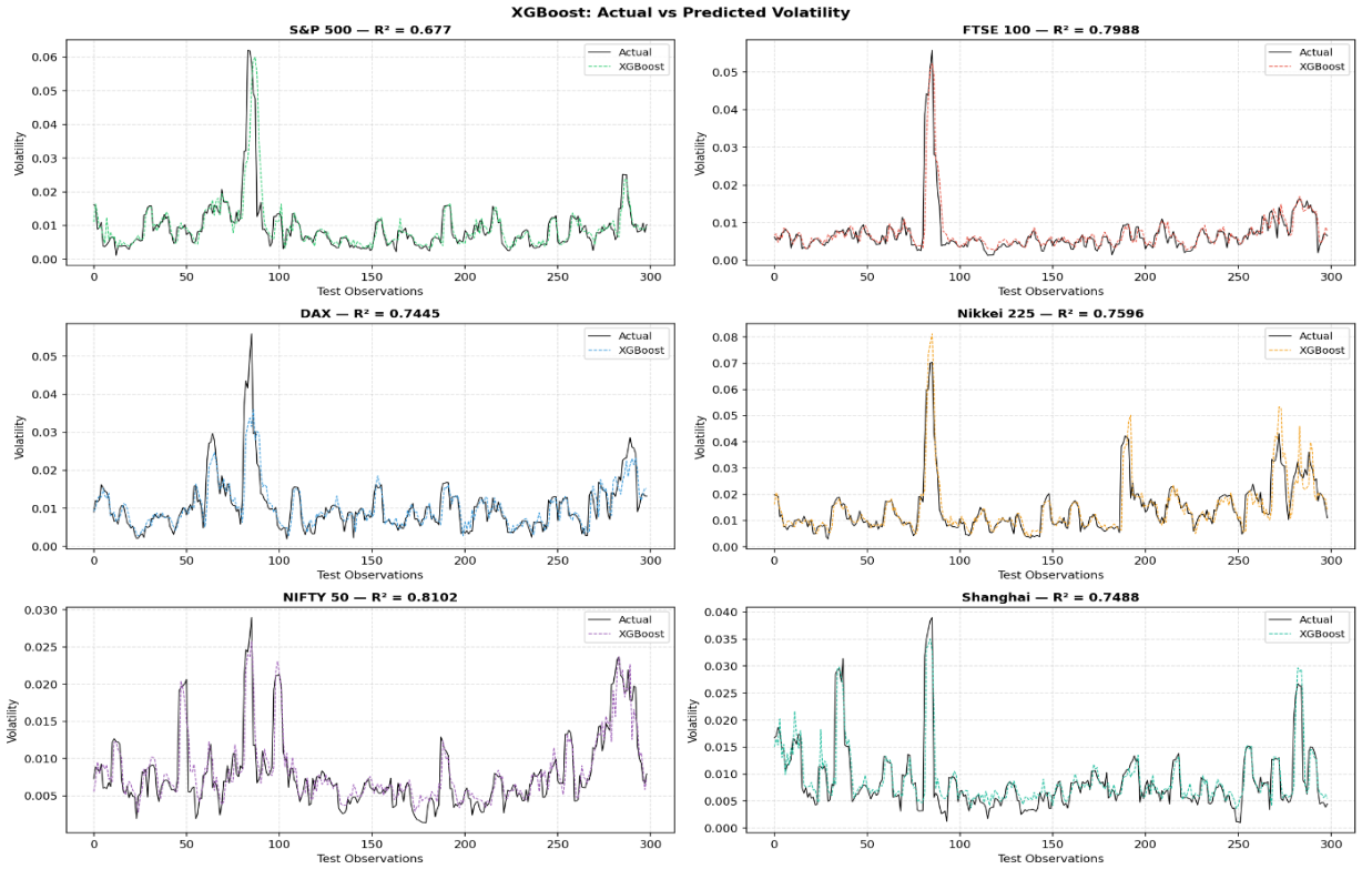
Figure 13.
SVR (RBF Kernel) — Actual vs Predicted Volatility (All Indices).
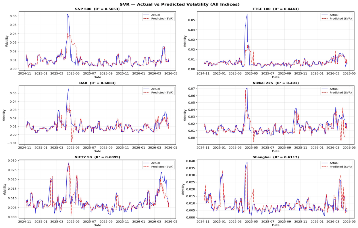

Table 1.
Descriptive Statistics of Daily Returns (2019–2026).
| Index | Mean | Std Dev | Min | Max | Skewness | Kurtosis |
|---|---|---|---|---|---|---|
| S&P 500 | 0.000753 | 0.013231 | -0.119845 | 0.095154 | -0.4954 | 14.5474 |
| FTSE 100 | 0.000334 | 0.011062 | -0.108745 | 0.090535 | -1.0623 | 15.8628 |
| DAX | 0.000618 | 0.013430 | -0.122386 | 0.109759 | -0.3666 | 12.5502 |
| Nikkei 225 | 0.000825 | 0.014767 | -0.123958 | 0.102263 | -0.2336 | 8.8303 |
| NIFTY 50 | 0.000607 | 0.011973 | -0.083019 | 0.087632 | -0.4969 | 9.4064 |
| Shanghai | 0.000385 | 0.011519 | -0.077244 | 0.080637 | -0.2117 | 7.8867 |
Table 2.
Mean Volatility by Period.
| Index | Pre-COVID | COVID | Post-COVID |
|---|---|---|---|
| S&P 500 | 0.006782 | 0.017065 | 0.009574 |
| FTSE 100 | 0.007198 | 0.016561 | 0.007447 |
| DAX | 0.008279 | 0.018416 | 0.009851 |
| Nikkei 225 | 0.007997 | 0.014412 | 0.012821 |
| NIFTY 50 | 0.008172 | 0.016425 | 0.008434 |
| Shanghai | 0.010454 | 0.011717 | 0.009231 |
Table 3.
ADF Test Results — All Indices (Full Period 2019–2026).
| Index | ADF Statistic | p-value | Critical Value (5%) | Conclusion |
|---|---|---|---|---|
| S&P 500 | -12.2750 | 0.0000 | -2.8635 | Stationary |
| FTSE 100 | -13.9235 | 0.0000 | -2.8635 | Stationary |
| DAX | -18.1788 | 0.0000 | -2.8635 | Stationary |
| Nikkei 225 | -40.3829 | 0.0000 | -2.8635 | Stationary |
| NIFTY 50 | -18.3011 | 0.0000 | -2.8635 | Stationary |
| Shanghai | -17.3197 | 0.0000 | -2.8635 | Stationary |
Table 4.
ARCH LM Test Results — Full Period (2019–2026).
| Index | LM Statistic | p-value | ARCH Effect |
|---|---|---|---|
| S&P 500 | 542.7528 | 0.0000 | Yes |
| FTSE 100 | 335.6808 | 0.0000 | Yes |
| DAX | 300.1867 | 0.0000 | Yes |
| Nikkei 225 | 296.5363 | 0.0000 | Yes |
| NIFTY 50 | 416.9230 | 0.0000 | Yes |
| Shanghai | 93.9947 | 0.0000 | Yes |
Table 5.
GARCH (1,1) Parameter Estimates — Full Period (2019–2026).
| Index | Ω | α | β | α+β | AIC | BIC |
|---|---|---|---|---|---|---|
| S&P 500 | 0.049552 | 0.164600 | 0.812964 | 0.977564 | 4285.25 | 4311.83 |
| FTSE 100 | 0.078224 | 0.178089 | 0.755415 | 0.933504 | 3817.34 | 3843.92 |
| DAX | 0.090367 | 0.162186 | 0.797783 | 0.959969 | 4509.25 | 4535.82 |
| Nikkei 225 | 0.240573 | 0.154734 | 0.728067 | 0.882800 | 5026.57 | 5053.15 |
| NIFTY 50 | 0.041948 | 0.096838 | 0.871168 | 0.968006 | 4154.36 | 4180.94 |
| Shanghai | 0.091812 | 0.079025 | 0.850744 | 0.929769 | 4302.77 | 4329.35 |
Table 6.
Volatility Persistence (α+β) by Period.
| Index | Pre-COVID | COVID | Post-COVID | Full Period |
|---|---|---|---|---|
| S&P 500 | 0.9154 | 1.0000 | 0.9678 | 0.9776 |
| FTSE 100 | 0.0367 | 0.9752 | 0.8157 | 0.9335 |
| DAX | 0.8830 | 1.0000 | 0.9226 | 0.9600 |
| Nikkei 225 | 0.2674 | 0.9947 | 0.7683 | 0.8828 |
| NIFTY 50 | 0.8995 | 1.0000 | 0.9683 | 0.9680 |
| Shanghai | 0.9863 | 0.9640 | 0.8194 | 0.9298 |
Table 7.
Random Forest Results — All Indices.
| Index | RMSE | MAE | R² Score |
|---|---|---|---|
| S&P 500 | 0.003699 | 0.001915 | 0.7709 |
| FTSE 100 | 0.002955 | 0.001563 | 0.7786 |
| DAX | 0.003513 | 0.002198 | 0.7621 |
| Nikkei 225 | 0.004451 | 0.002757 | 0.8052 |
| NIFTY 50 | 0.002337 | 0.001470 | 0.7907 |
| Shanghai | 0.003351 | 0.001935 | 0.6992 |
| Mean | 0.003384 | 0.001973 | 0.7678 |
Table 8.
XGBoost Results — All Indices.
| Index | RMSE | MAE | R² Score |
|---|---|---|---|
| S&P 500 | 0.004460 | 0.002269 | 0.6770 |
| FTSE 100 | 0.003069 | 0.001517 | 0.7988 |
| DAX | 0.004221 | 0.002465 | 0.7445 |
| Nikkei 225 | 0.005367 | 0.003126 | 0.7596 |
| NIFTY 50 | 0.002535 | 0.001672 | 0.8102 |
| Shanghai | 0.003548 | 0.002108 | 0.7488 |
| Mean | 0.003867 | 0.002193 | 0.7565 |
Table 9.
SVR (RBF Kernel) Results — All Indices.
| Index | RMSE | MAE | R² Score |
|---|---|---|---|
| S&P 500 | 0.005090 | 0.002464 | 0.5653 |
| FTSE 100 | 0.004666 | 0.001895 | 0.4443 |
| DAX | 0.004494 | 0.002651 | 0.6083 |
| Nikkei 225 | 0.007176 | 0.004100 | 0.4910 |
| NIFTY 50 | 0.002836 | 0.001665 | 0.6899 |
| Shanghai | 0.003817 | 0.002261 | 0.6117 |
| Mean | 0.004680 | 0.002506 | 0.5851 |
Table 10.
Model Comparison — Random Forest vs XGBoost vs SVR (All Metrics).
| Index | RF RMSE | RF MAE | RF R² | XGB RMSE | XGB MAE | XGB R² | SVR RMSE | SVR MAE | SVR R² |
|---|---|---|---|---|---|---|---|---|---|
| S&P 500 | 0.003699 | 0.001915 | 0.7709 | 0.004460 | 0.002269 | 0.6770 | 0.005090 | 0.002464 | 0.5653 |
| FTSE 100 | 0.002955 | 0.001563 | 0.7786 | 0.003069 | 0.001517 | 0.7988 | 0.004666 | 0.001895 | 0.4443 |
| DAX | 0.003513 | 0.002198 | 0.7621 | 0.004221 | 0.002465 | 0.7445 | 0.004494 | 0.002651 | 0.6083 |
| Nikkei 225 | 0.004451 | 0.002757 | 0.8052 | 0.005367 | 0.003126 | 0.7596 | 0.007176 | 0.004100 | 0.4910 |
| NIFTY 50 | 0.002337 | 0.001470 | 0.7907 | 0.002535 | 0.001672 | 0.8102 | 0.002836 | 0.001665 | 0.6899 |
| Shanghai | 0.003351 | 0.001935 | 0.6992 | 0.003548 | 0.002108 | 0.7488 | 0.003817 | 0.002261 | 0.6117 |
| Mean | 0.003384 | 0.001973 | 0.7678 | 0.003867 | 0.002193 | 0.7565 | 0.004680 | 0.002506 | 0.5851 |
Disclaimer/Publisher’s Note: The statements, opinions and data contained in all publications are solely those of the individual author(s) and contributor(s) and not of MDPI and/or the editor(s). MDPI and/or the editor(s) disclaim responsibility for any injury to people or property resulting from any ideas, methods, instructions or products referred to in the content. |
© 2026 by the authors. Licensee MDPI, Basel, Switzerland. This article is an open access article distributed under the terms and conditions of the Creative Commons Attribution (CC BY) license (http://creativecommons.org/licenses/by/4.0/).
Copyright: This open access article is published under a Creative Commons CC BY 4.0 license, which permit the free download, distribution, and reuse, provided that the author and preprint are cited in any reuse.