Hecke Transport of Conifold Mixed-Hodge Extensions: Localized Survival and Higher Derived Attachments

1. Introduction

1.1. Motivation: Singular Hodge Data Under Hecke Modification

The functorial transport of singular mixed-Hodge data through a Hecke correspondence is sensitive to  maps , not only to direct-image objects. A short exact sequence in mixed Hodge modules, $0\to I\to P\to R\to 0$, carries a connecting morphism $ϵ:R\to I\left[1\right]$ that is invisible in the additive identity $\left[P\right]=\left[I\right]+\left[R\right]$ in $K_0$. An exact derived correspondence functor preserves its distinguished triangle, but can annihilate the connecting morphism even when none of the three transported objects vanishes. Nearby and vanishing cycles contribute their own canonical, variation, and monodromy maps, with types and Tate twists that cannot be inferred from the numerical decomposition of stalks [1,2,3,4,5].

The source of our calculation is the  corrected forward  conifold mixed-Hodge extension developed in [6,7], not a hypothetical extension inferred from conifold topology. We attach it to the actual lower elementary $G{L}_2$ Hecke correspondence on Higgs bundles by smooth evaluation into the universal determinant singularity $X=\{\det A=0\}\subset \mathrm{End}\left({\mathbb{C}}^2\right)$. This gives a geometrically defined source realization, retains the varying invariant line and its framing groupoid, and produces a specified morphism before and after target pushforward. An arbitrary global nodal threefold $X_0$ requires an additional source-realization functor; the local construction does not supply one automatically.

Three geometric mechanisms enter. The determinant on invariant-line incidence factors as a normal crossing $\alpha \delta$ whose components are the kernel- and image-line small resolutions. Their intersection is the $A_1$ Springer resolution; it is also the transverse slice of bounded two-step minuscule $G{L}_2$ convolution [8,9,10]. On the source-node stratum the modified Higgs value is controlled by a first-jet quadratic in $H^0({\mathbb{P}}^1,{\mathcal{O}}_{{\mathbb{P}}^1}\left(2\right)\otimes K_z^{\otimes 2})$. Finally, on the kernel-line small resolution the corrected extension becomes a codimension-two Gysin morphism. The  auxiliary  projection to the line parameter space kills it under $R{q}_{*}$ but detects it under $R{q}_{!}$. This is a diagnostic of information loss, not the result for the genuine modified-Higgs target.

The central result comes from the genuine unframed correspondence. Over an admissible rank-one target open  U , the intrinsic image line recovers the inverse upper modification on the kernel branch. Its source-node locus becomes a regular codimension-two immersion, and the selected equivariant Gysin morphism survives both ordinary and exceptional target direct images (Theorem 8). A stronger conclusion holds on the saturated open $U^{\prime }\subset U$: the  complete  inverse-eigenline correspondence is a finite flat double cover, and the transported class has a nonzero degree-two derived realization with explicit perverse Postnikov placement, subject to the quotient-stack MHM comparison hypotheses (Theorem 9). These statements distinguish the genuine Hecke map, its nonproper framing atlas, and the auxiliary line-projection benchmark.

Our motivation also interfaces with the author’s singular Hodge-atom and BPS program [11] and with geometric Hecke operators in the Kapustin–Witten picture [12]. Neither physical line operators nor a spectral-atom realization is identified here; the object of study is the corrected MHM extension and its specified geometric transport.

1.2. The Corrected Conifold Coefficient

Let $\pi :\mathcal{X}\to \mathsf{\Delta }$ be a one-parameter degeneration of smooth complex threefolds whose reduced central fiber $X_0$ has ordinary double points $\mathsf{\Sigma }=\{p_1,\dots ,p_r\}$. For the inclusions $i_k:\left\{p_k\right\}\hookrightarrow X_0$, the corrected source package of [6,7] is

$$I^H:={\mathrm{IC}}_{X_0}^H,R_{\mathsf{\Sigma }}^H:={\displaystyle \underset{k=1}{\overset{r}{⨁}}}{i}_{k*}{\mathbb{Q}}_{\left\{p_k\right\}}^H(-2),$$

(1)

together with the specified short exact sequence in $\mathrm{MHM}\left(X_0\right)$

$$0⟶I^H\stackrel{a}{\to }{P}^H\stackrel{b}{\to }{R}_{\mathsf{\Sigma }}^H⟶0.$$

(2)

Its forward Yoneda class is represented by

$$\left[{ϵ}_{\mathsf{\Sigma }}\right]\in {\mathrm{Ext}}_{\mathrm{MHM}\left(X_0\right)}^1(R_{\mathsf{\Sigma }}^H,I^H),{ϵ}_{\mathsf{\Sigma }}:R_{\mathsf{\Sigma }}^H⟶I^H\left[1\right].$$

(3)

The subobject is $I^H$, the quotient is $R_{\mathsf{\Sigma }}^H$, and $P^H$ is the already corrected mixed-Hodge coefficient; it is not defined here by an uncorrected variation cone.

The node-interface object has a different Tate normalization:

$$Q_{\mathsf{\Sigma }}^H:={\displaystyle \underset{k=1}{\overset{r}{⨁}}}{i}_{k*}{\mathbb{Q}}_{\left\{p_k\right\}}^H(-1).$$

(4)

For the perverse-normalized unipotent nearby and vanishing Hodge modules, we write

$${\mathsf{\Psi }}^H\stackrel{{\mathrm{can}}^H}{\to }{\mathsf{\Phi }}^H\stackrel{{\mathrm{Var}}^H}{\to }{\mathsf{\Psi }}^H(-1),N^H={\mathrm{Var}}^H\circ {\mathrm{can}}^H.$$

(5)

The weights of ${\mathbb{Q}}^H(-1)$ and ${\mathbb{Q}}^H(-2)$ are 2 and 4. The monodromy factorization through $Q_{\mathsf{\Sigma }}^H$, where supplied by the source construction, is therefore kept apart from the forward extension. The input is the morphism-bearing package

$${\mathfrak{A}}_{X_0}^H:=(I^H,P^H,R_{\mathsf{\Sigma }}^H,{ϵ}_{\mathsf{\Sigma }};{\mathsf{\Psi }}^H,{\mathsf{\Phi }}^H,{\mathrm{can}}^H,{\mathrm{Var}}^H,N^H),$$

(6)

with the node-interface factorization retained as additional specified data. Local node contributions are not identified with their globally independent vanishing-cycle span: relations among the vanishing cycles remain possible.

For the incidence calculations, $X=\{\det A=0\}$ is the universal local conifold, with selected nonzero generator ${ϵ}_X:i_{o*}{\mathbb{Q}}^H(-2)\to {\mathrm{IC}}_X^H\left[1\right]$. A global $X_0$ requires a separate source realization.

1.3. The Geometric Hecke Transport Problem

Let  C  be a smooth projective complex curve, $z\in C$ a marked point, and $(E_{-},{\theta }_{-})$ a rank-two Higgs bundle. For a line $\ell \subset {\left(E_{-}\right)}_z$, the lower elementary modification is

$$0⟶E_{+}⟶E_{-}⟶{\left(E_{-}\right)}_z/\ell ⟶0.$$

(7)

The field ${\theta }_{+}$ is regular precisely when ${\theta }_{-}\left(z\right)\ell \subseteq \ell$. Its leading value depends on the first source Higgs jet and its complete first jet on the second. The genuine correspondence is

$$Y_{-}\stackrel{p}{\leftarrow }{\mathcal{H}}_z\stackrel{q}{\to }{Y}_{+},$$

(8)

with distinct invariant-line, framed-jet, and unframed stack levels.

Write $K_z=T_z^{*}C$, $S=\ell$, $Q={\left(E_{-}\right)}_z/\ell$, and $F=E_{+}$. The modified fiber fits into the canonical exact sequence $0\to Q\otimes K_z\to F_z\to S\to 0$ (Lemma 13). For the induced target line ${\ell }_{+}=Q\otimes K_z$, the eigenvalues on the marked line and quotient exchange: ${\alpha }_{+}={\delta }_{-}$ and ${\delta }_{+}={\alpha }_{-}$ (Proposition 27). On ${\theta }_{-}\left(z\right)=0$, the potentially nonzero target value is the intrinsic quadratic section of Proposition 28; its roots encode the invariant lines of the first source jet.

On a nonempty stable-bundle locus satisfying $H^0(C,{\mathrm{End}}_0{E}_{-}\left(z\right))=0$, framed Higgs evaluation $e:{\mathcal{Y}}_{-}^{\mathrm{fr}}\to \mathrm{End}\left({\mathbb{C}}^2\right)$ is smooth and surjective. Its incidence base change is Cartesian and defines the genuine modified-Higgs map $q_{+}$ to the Higgs moduli stack (Section 4.6). The stronger first-jet evaluation condition is

$$h^0(C,{\mathcal{O}}_C\left(2z\right))=1,H^0(C,{\mathrm{End}}_0{E}_{-}\left(2z\right))=0.$$

Section 4.6 proves existence for every odd-degree determinant when $g\ge 3$ and $h^0\left({\mathcal{O}}_C\left(2z\right)\right)=1$, as well as for even-degree determinants when $g\ge 4$ or when $g=3$ and $4z\neg \sim K_C$. The genus-three even-degree theta-characteristic case $4z\sim K_C$ is obstructed; genus two is excluded by Riemann–Roch. These existence assertions use the specified curve and marked-point hypotheses, not an unconditional statement for arbitrary $C,z$.

On the rank-one target open, the intrinsic line ${\ell }_{+}=K_z^{-1}\mathrm{im}{\theta }_{+}\left(z\right)$ canonically determines the inverse upper modification on the kernel branch. The decisive map is an isomorphism of  unframed  moduli groupoids, not an inverse to the framing-forgetting torsor. The complete inverse incidence has two scheme-theoretic eigenlines away from the nilpotent locus and a length-two nonreduced fiber at a nonzero nilpotent value. Imposing admissibility of  both  inverse sources gives a saturated open $U^{\prime }\subset U$ over which the full correspondence is finite locally free of degree two (Proposition 59).

For a chosen source realization $\mathsf{S}$, kernel $\mathcal{K}$, and bounded six-functor operations, write

$$\mathsf{H}\left(F\right)=R{q}_{\diamond }\left(p^{*}\mathsf{S}\left(F\right)\otimes \mathcal{K}\right)\left[d\right]\left(m\right),\diamond \in \{*,!\}.$$

(9)

The choice of direct image, shift and Tate twist is part of the specified correspondence, not inferred from a desired result. The local class survives evaluation and incidence pullback, and its genuine unit-kernel target images are nonzero on  U . On the smaller saturated $U^{\prime }$, finite pushforward and the perverse-degree calculation identify their common derived attachment as a nonzero element of ${\mathrm{Hom}}_{{\mathsf{D}}_H\left(U^{\prime }\right)}(R^{\prime },I^{\prime }\left[2\right])$, with the exact equivariant normalization stated in Theorem 9. Outside these opens, or for an unrelated realization or general kernel, the image remains a separate morphism-level problem.

1.4. Principal Results and Proof Strategy

The central assertions are localized derived survival on  U  and the nonzero degree-two extension on $U^{\prime }$. The geometric input, first-jet existence theorem, and auxiliary Gysin calculation are stated separately; Springer convolution and conditional fusion supply a bounded comparison. We distinguish a proved result from a theorem subject to specified quotient-stack MHM or specialization-exchange hypotheses, and do not assert complete global perverse amplitudes or arbitrary-kernel transport.

Proposition 1

(Invariant-line incidence and its Springer intersection).  Let $M={\mathrm{Mat}}_2\left(\mathbb{C}\right)$, $X=\{A\in M:\det A=0\}$, and $\mathcal{I}=\{(A,\ell ):A\ell \subseteq \ell \}\subset M\times {\mathbb{P}}^1$. The projection $p:\mathcal{I}\to M$ is projective, $\mathcal{I}$ is a smooth fourfold, and $\det \circ p=\alpha \delta$ in adapted coordinates. The central fiber is the normal-crossing union of the kernel-line and image-line small resolutions, meeting in $Z\simeq {\mathrm{Tot}}_{{\mathbb{P}}^1}\mathcal{O}(-2)$. The induced $Z\to \mathcal{N}$ is the minimal $A_1$ Springer resolution; its direct image contains a point-supported ${\mathbb{Q}}^H(-1)$ term, distinct from the determinant vanishing-cycle contribution ${\mathbb{Q}}^H(-2)$. 

These assertions follow from Propositions 16, 18, and 20.

Lemma 1

(Transport of a distinguished extension).  If an exact derived correspondence functor $\mathsf{H}:{\mathsf{D}}_H\left(X_0\right)\to {\mathsf{D}}_H\left(Y_{+}\right)$ is defined on the corrected source triangle, then 

$$\mathsf{H}\left(I^H\right)⟶\mathsf{H}\left(P^H\right)⟶\mathsf{H}\left(R_{\mathsf{\Sigma }}^H\right)\stackrel{\mathsf{H}\left({ϵ}_{\mathsf{\Sigma }}\right)}{\to }\mathsf{H}\left(I^H\right)\left[1\right]$$

(10)

 is distinguished and splits exactly when $\mathsf{H}\left({ϵ}_{\mathsf{\Sigma }}\right)=0$. If both endpoints lie in $\mathrm{MHM}\left(Y_{+}\right)$, the triangle is a heart-level Yoneda extension; otherwise its connecting arrow is retained with its derived Postnikov data. 

This is Proposition 38 and Lemma 22.

Theorem 1

(Evaluation-regular conifold–Hecke realization, branch exchange, and first-jet existence).  On a nonempty locus of framed stable bundles satisfying $H^0(C,{\mathrm{End}}_0{E}_{-}\left(z\right))=0$, framed Higgs evaluation $e:{\mathcal{Y}}_{-}^{\mathrm{fr}}\to M$ is smooth and surjective. The varying-line correspondence ${\mathcal{H}}^{\mathrm{fr}}={\mathcal{Y}}_{-}^{\mathrm{fr}}{\times }_M\mathcal{I}$ and its determinant restriction are Cartesian, and elementary lower modification defines an algebraic map to the modified-Higgs stack. 

 The modified fiber fits into $0\to Q\otimes K_z\to {\left(E_{+}\right)}_z\to S\to 0$; its marked eigenvalues satisfy ${\alpha }_{+}={\delta }_{-}$ and ${\delta }_{+}={\alpha }_{-}$. On the source-node fiber $T\times {\mathbb{P}}^1$ the transformed leading Higgs value is nilpotent, with its potentially nonzero component a section of ${\mathcal{O}}_{{\mathbb{P}}^1}\left(2\right)\otimes K_z^{\otimes 2}$. Its root scheme is ${\mathbb{P}}^1$ for a scalar source first jet, two reduced points for distinct eigenvalues, and one length-two nonreduced point for a nonscalar repeated eigenvalue. 

 If $g\ge 3$ and $h^0(C,{\mathcal{O}}_C\left(2z\right))=1$, first-jet evaluation-regular stable bundles exist with every prescribed odd-degree determinant . They also exist with prescribed even-degree determinant for $g\ge 4$, and for $g=3$ provided $4z\neg \sim K_C$. For $g=3$ and $4z\sim K_C$, the even-degree vanishing is obstructed; for $g=2$ it is impossible. In the existence ranges there are Higgs fields with ${\theta }_{-}\left(z\right)=0$ and nonzero intrinsic quadratic, and hence admissible regular-nilpotent target values. 

The incidence, intrinsic fiber, and marked branch calculations are proved in Propositions 23, 24, 27, and 28. The first-jet criterion and existence results are Lemma 11, Theorems 6 and 7, and Corollary 3. The target and source branches are  marked ; the result is neither a flop equivalence nor a realization of an arbitrary global nodal $X_0$.

Theorem 2

(Derived reconstruction and local Gysin transport).  For the kernel-line small resolution $X\stackrel{m}{\leftarrow }\tilde{X}\stackrel{q_{\mathrm{line}}}{\to }{\mathbb{P}}^1$, the nonzero local forward class pulls back to a nonzero scalar multiple $\gamma g_E$ of the codimension-two Gysin morphism, where $\gamma \in {\mathbb{Q}}^{\times }$. Its direct images satisfy $R{q}_{\mathrm{line}*}{m}^{*}{ϵ}_X=0$ and $R{q}_{\mathrm{line}!}{m}^{*}{ϵ}_X\ne 0$. The stalk, costalk, perverse-degree, and boundary-residual calculations identify the two outcomes. For a verified Hecke transform, recollement, MacPherson–Vilonen attaching maps, and Hom/Ext constraints govern its target arrow without reducing that arrow to the endpoint multiplicities. 

The local morphism calculations are Propositions 31 and 33; the derived reconstruction is in Section 6. The octahedral comparison morphism is not identified with the forward Yoneda class.

Proposition 2

(Fixed-source Hecke curves and Higgs normal data).  For a fixed stable $E_{-}$ satisfying $H^0(C,{\mathrm{End}}_0{E}_{-}\left(z\right))=0$, the elementary Hecke curve is pointwise noncontracted and infinitesimally injective in the bundle moduli stack, even when the source Higgs first jet is scalar. Its determinant is $\det F_{\ell }\simeq \det E_{-}\otimes {\mathcal{O}}_C(-z)$. When $\mathrm{deg}{E}_{-}$ is even, all modified bundles are stable; the Hecke curve embeds in the stable-bundle moduli space, and its normal bundle in the stable-underlying-bundle Higgs locus has rank $8g-7$ and determinant ${\mathcal{O}}_{{\mathbb{P}}^1}(-2)$. 

The noncontraction geometry is classical [13,14,15,16]. The explicit differential and normal calculations needed here are Propositions 51– 53; by themselves they do not establish survival of a Hecke-pushed MHM extension.

Theorem 3

(Localized survival of the forward class on the genuine Hecke target).  Let U be the admissible rank-one target open of Proposition 55, meeting the source-node image. The distinguished target line is reconstructed from ${\ell }_{+}=K_z^{-1}\mathrm{im}{\theta }_{+}\left(z\right)$, and the inverse upper modification is an isomorphism of unframed kernel-branch Hecke groupoids over U. The source-node image is a regular codimension-two immersion. For the unit Hecke kernel, the selected equivariant lift of the nonzero universal determinant-conifold forward class, and the compatible mixed-Hodge normalization, its two genuine target images satisfy 

$${\left.R{q}_{+,0*}\left(p_{-,0}^{*}{e}_0^{*}{ϵ}_X\left[r\right]\right)\right|}_U\ne 0,{\left.R{q}_{+,0!}\left(p_{-,0}^{*}{e}_0^{*}{ϵ}_X\left[r\right]\right)\right|}_U\ne 0.$$

(11)

 Both transformed distinguished triangles are derived nonsplit on U. The first-jet existence theorem supplies a nonempty such node image in its stated genus and determinant ranges. Neither conclusion refers to the auxiliary line projection or to an unrelated global nodal source. 

The decisive inputs are the actual rank-one branch inverse, the equivariant forward costalk lift, and the closed-branch Gysin detector (Proposition 55 and Lemmas 23, 25). Their combination is Theorem 8; Corollary 7 supplies nonempty global Higgs examples. No perverse-heart concentration follows from derived nonsplitting alone.

Theorem 4

(Finite degree-two transport and the higher extension class).  Let $U^{\prime }\subset U$ be the nonempty saturated admissible open of Proposition 59. The complete unframed inverse-eigenline correspondence $q^{\prime }{:\mathcal{E}|}_{U^{\prime }}\to U^{\prime }$ is finite locally free of degree two; its two inverse eigenlines merge into a length-two scheme over the nonzero nilpotent locus. In particular, $R{q}_{!}^{\prime }\simeq R{q}_{*}^{\prime }$ on the selected coefficients. 

 Assume the unit kernel and the equivariant quotient-stack MHM formalism, descent comparison, and normalized smooth-atlas exchange specified in Theorem 9. Writing $I^{\prime }$ and $R^{\prime }$ for the two transported perverse objects, the connecting arrow is a nonzero higher extension 

$$0\ne \left[{ϵ}_{U^{\prime }}\right]\in {\mathrm{Hom}}_{{\mathsf{D}}_H\left(U^{\prime }\right)}(R^{\prime },I^{\prime }\left[2\right]).$$

(12)

 Its middle coefficient $P^{\prime }$ has 

$${}^p{\mathcal{H}}^0\left(P^{\prime }\right)\simeq I^{\prime },{}^p{\mathcal{H}}^1\left(P^{\prime }\right)\simeq R^{\prime },{}^p{\mathcal{H}}^n\left(P^{\prime }\right)=0(n\notin \{0,1\}),$$

(13)

 and $\left[{ϵ}_{U^{\prime }}\right]$ is their nontrivial Postnikov attachment. These are statements about a finite unframed correspondence, not about a finite framing atlas or an unconditional global Hecke functor. 

The source-side perverse calculation on the  complete  reducible incidence fiber is Proposition 30 and Corollary 4. Finite transport, nonvanishing, and compatible smooth-atlas witnesses are proved in Theorem 9 and Corollary 9. The source forward Yoneda ${\mathrm{Ext}}^1$ and this target degree-two derived morphism are not identified as heart-level short exact sequences.

Theorem 5

(Springer slice and extension-sensitive bounded convolution).  The Springer resolution $Z\simeq {\mathrm{Tot}}_{{\mathbb{P}}^1}\mathcal{O}(-2)$ is the Cartesian pullback of the bounded two-step $G{L}_2$ affine-Grassmannian convolution resolution to the nilpotent $A_1$ transverse slice. The full convolution surface is ${\mathbb{F}}_2$, while the Springer slice is nonproper. The point-supported pure Hodge term has Tate type ${\mathbb{Q}}^H(-1)$, distinct from the source forward quotient ${\mathbb{Q}}^H(-2)$. 

 For selected Hecke kernels satisfying the support, base-change and family-specialization hypotheses of Theorem 13, the natural equivalence $\mathsf{\Theta }:{\mathsf{H}}_2\circ {\mathsf{H}}_1\stackrel{\sim }{\to }{\mathsf{H}}_{21}$ satisfies 

$${\mathsf{\Theta }}_{I^H}\left[1\right]\circ ({\mathsf{H}}_2\circ {\mathsf{H}}_1)\left({ϵ}_{\mathsf{\Sigma }}\right)={\mathsf{H}}_{21}\left({ϵ}_{\mathsf{\Sigma }}\right)\circ {\mathsf{\Theta }}_{R_{\mathsf{\Sigma }}^H}.$$

(14)

 Its family comparison also intertwines ${\mathrm{can}}^H$, ${\mathrm{Var}}^H$, and $N^H$ with the appropriate Tate twist. This formal compatibility does not assert nonvanishing of the image. 

The geometric statements are Theorem 12, Corollary 12, and Lemma 32. The derived fusion theorem is conditional on the specified correspondence and kernel exchanges in Section 9.

1.5. Relation to the Existing Literature

The argument draws on intersection complexes and perverse gluing [1,4,5], Saito’s mixed Hodge modules and specialization functors [2,3], and the classical topology of isolated singularities and monodromy [17,18]. Springer geometry and type- A  affine Grassmannians supply the small-resolution and lattice frameworks [8,19] and [9,10]; see also [20]. The present problem is not to reprove the general theory, but to retain its morphisms and Tate normalizations for one corrected singular coefficient.

Hodge refinements of Satake and convolution.

Fedorov’s Hodge-theoretic Satake equivalence [21] equips spherical convolution with a tensor formalism for equivariant polarizable pure Hodge modules. Its purity and semisimplicity are important normalization checks, but do not transport an arbitrary nonsplit  mixed  conifold extension into a pure heart. The motivic Satake construction of Richarz and Scholbach [22] offers a complementary six-functor and Tate-sensitive framework. Cautis, Dodd, and Kamnitzer [23] study associated-graded Hodge modules and categorical ${\mathfrak{sl}}_2$ structures; associated-graded identifications do not recover the connecting Yoneda arrow. The Springer $\mathbb{Q}(-1)$ summand remains distinct from the forward $\mathbb{Q}(-2)$ quotient.

Specialization and centrality.

Gaitsgory’s nearby-cycle construction of central sheaves [24] motivates the compatibility problem between specialization and affine-Hecke composition. Higher unipotent nearby cycles and their iteration comparisons in Achar–Riche [25,26] supply the relevant exchange machinery, but such comparisons require their precise existence and base-change hypotheses; they are not uniform isomorphisms for arbitrary singular coefficients. Salmon’s general-base analysis [27] provides related specialization context. At the diagrammatic level, Elias [28] constructs centrality-related chain complexes and compatibility data in affine Soergel settings. That work underscores why natural maps and homotopies, rather than only matching objects, are essential to convolution coherence. Here the maps are constructed using MHM adjunction, recollement, and proper base change, with no claim to a new central object.

Classical Hecke curves and genuine Hecke–Higgs geometry.

Elementary modification curves on moduli of stable bundles are classical: Narasimhan–Ramanan’s Hecke-cycle geometry [13], Hwang’s tangent-vector calculations [14], Hwang–Ramanan’s relation to the Hitchin discriminant [15], and Sun’s minimal rational-curve results [16] provide the appropriate precedents. In particular, Hwang–Ramanan [15] prove relevant generic vanishings for twisted traceless endomorphisms in higher genus. Our fixed-point and genus-three parity refinements are used to establish the required first-jet evaluation locus, not to claim discovery of generic vanishing or the underlying Hecke curve. Our fixed-source rigidity argument is used to control the additional Higgs deformation and the correction from noncontraction to the  rank-one inverse  needed for the selected extension morphism. The fixed-determinant identity is retained, while normal-data assertions are made only under the stability and degree conditions stated in Section 7.

Donagi, Pantev, and Simpson [29] study rank-two Hecke–Higgs geometry with rigidifications, spectral and Prym structures, and direct-image calculations. Their work is the closest geometric comparator for a true modified-Higgs target, but does not compute the image of our selected conifold Yoneda class. The lower modification and invariant-line orientation must also be compared with [30]; related extended-Bogomolny geometry is described in [31]. The equivariant mixed-Hodge comparison is formulated in the selected stack-theoretic six-functor framework [32]. Crucially, the finite inverse-eigenline correspondence is defined  after  unframed descent; there is no finiteness claim for the higher-jet framing group. Smooth-atlas pullback is normalized separately from finite direct image.

Theta-characteristic obstruction.

The exceptional even-degree genus-three first-jet phenomenon is governed by the parity result for orthogonal bundles and theta characteristics [33]. Section 4.6 spells out the obstruction and constructive nonemptiness conditions; they are not inferred from a generic-dimension count.

BPS and geometric Langlands interfaces.

The geometric-Langlands framework of [34] and the Kapustin–Witten line-operator picture [12] explain why a morphism-sensitive Hecke calculus may have broader significance. The Hecke operators on BPS cohomology studied by Davison and collaborators [35] concern different moduli spaces, coefficients, and operator constructions; no identification with our conifold extension is used. The author’s singular Hodge-atom work supplies the conifold and global-gluing input [6,7] and [11,36], while  Bivariant Hodge Atoms I  supplies a separate Hecke collision benchmark [37]. The contribution is the evaluation-based incidence realization of the corrected extension, intrinsic marked branch exchange, and explicit first-jet existence ranges; the localized survival of its actual unit-kernel target morphism; and, on the finite saturated open, the nonzero degree-two extension controlling the perverse Postnikov attachment. The Springer–convolution slice remains a distinct geometric and representation-theoretic comparison.

1.6. Notation and Conventions

All varieties, curves, and algebraic stacks are over $\mathbb{C}$; $\mathbb{Q}$, $\mathbb{Z}$, and $\mathbb{R}$ denote the usual coefficient rings. The degeneration parameter is  t  (or  s  for a specified family); $z\in C$ is the Hecke point,  w  its local parameter, and $K_z=T_z^{*}C$ its cotangent line. The conifold node set is $\mathsf{\Sigma }$, while  X  is the local determinantal model and $X_0$ a central fiber of a possibly unrelated degeneration. The maps $a,b$ denote the source extension arrows; $p,q$ denote correspondence projections with subscripts indicating which correspondence is intended.

For a finite-type variety  Z , put ${\mathsf{D}}_H\left(Z\right):=D^b\mathrm{MHM}\left(Z\right)$, with heart $\mathrm{MHM}\left(Z\right)$ and perverse cohomology ${}^p{\mathcal{H}}^n$. The rational realization is $\mathrm{rat}:\mathrm{MHM}\left(Z\right)\to \mathrm{Perv}(Z;\mathbb{Q})$. On a smooth  d -fold, ${\mathbb{Q}}_Z^H\left[d\right]$ is perverse normalized, and ${\mathrm{IC}}_Z^H$ is the intersection-complex Hodge module. We write $\left[n\right]$ for cohomological shifts and $\left(m\right)$ for Tate twists. Derived pullback, ordinary and exceptional pushforward, and extraordinary pullback are $f^{*}$, $R{f}_{*}$, $R{f}_{!}$, and $f^{!}$; $R{f}_{*}$ and $R{f}_{!}$ are not identified for nonproper maps. The equalities ${\mathrm{Ext}}_{\mathrm{MHM}\left(Z\right)}^n(A,B)={\mathrm{Hom}}_{{\mathsf{D}}_H\left(Z\right)}(A,B\left[n\right])$ are used for heart objects and $n\ge 0$.

We reserve ${ϵ}_{\mathsf{\Sigma }}$ for the forward extension and ${\omega }_{u,v}$ for an octahedral connecting arrow. The maps ${\mathrm{can}}^H$, ${\mathrm{Var}}^H$, and $N^H$ retain their normalization in (5). The symbol $q_{\mathrm{line}}$ is reserved for the small-resolution projection to ${\mathbb{P}}^1$, while $q_{+}$ denotes an actual modified-Higgs map. Superscripts $\mathrm{fr}$ and $\mathrm{unfr}$ distinguish fiber- or jet-framing atlases from quotient-stack coefficients. The admissible rank-one target open is  U  when the context is the kernel-branch inverse, and $U^{\prime }\subset U$ is its saturated admissible finite-cover open. Neither should be confused with the complement $U_Y$ of an arbitrary recollement stratum. We write $q^{\prime }$ for the finite unframed inverse incidence on $U^{\prime }$, never for the nonproper target framing atlas. All stack-level MHM operations and smooth-atlas normalizations are made in a specified compatible formalism [32].

1.7. Organization of the Paper

Section 2 fixes the conifold extension and MHM normalizations. Section 3 and Section 4 construct the invariant-line modification, smooth evaluation realization, and Cartesian correspondence. Section 5 computes the local Gysin and ordinary/exceptional pushforward contrast; Section 6 retains the varying-line transport and derived gluing maps. Section 7 and Section 8 compute the Hecke-curve and inverse-fiber geometry, prove localized survival on  U , establish finite degree-two transport and the degree-two derived result on $U^{\prime }$, and verify normalized framing compatibility. Section 9 proves the Springer–convolution slice identification and formulates the specialization-compatible bounded fusion result; Section 10 records the consequences. The appendices preserve coordinate, Hodge-degree, cone, and map-index verification data.

2. Conifold Mixed-Hodge Modules and Hecke Foundations

We fix the corrected forward conifold extension, its separate nearby/vanishing-cycle interface, and the mixed-Hodge-module conventions for the actual Hecke correspondence. The local costalk, functorial, recollement, and lower-modification normalizations are specified here; Section 4.6 proves first-jet existence in explicit genus and determinant ranges. We distinguish three increasingly stronger assertions for the universal determinant conifold: nonzero incidence pullback, localized unit-kernel survival on the unframed modified-Higgs target  U , and finite degree-two transport on a smaller admissible open $U^{\prime }$, where the surviving arrow has a specified degree-two derived placement. None gives an automatic transform of an unrelated global nodal coefficient. We use the conventions of Section 1.6.

2.1. One-Parameter Conifold Degenerations

Definition 1

(Nodal degeneration).  Let Δ be a sufficiently small complex disk with coordinate t. A nodal threefold degeneration is a proper flat morphism $\pi :\mathcal{X}\to \mathsf{\Delta }$ whose general fiber $X_t$ is a smooth complex threefold and whose reduced central fiber $X_0$ has finitely many ordinary double points $\mathsf{\Sigma }=\{p_1,\dots ,p_r\}$. Whenever constant pure Hodge coefficients on the total space are used, assume that $\mathcal{X}$ is smooth of complex dimension four near $X_0$, and that the local family at each node is analytically equivalent to 

$$\pi (x_1,x_2,x_3,x_4)=x_1^2+x_2^2+x_3^2+x_4^2=t.$$

(15)

 Write $U=X_0\setminus \mathsf{\Sigma }$, with inclusions $j:U\hookrightarrow X_0$, $i_k:\left\{p_k\right\}\hookrightarrow X_0$, and $i:\mathsf{\Sigma }\hookrightarrow X_0$. 

Remark 1

(Local and global vanishing cycles).  The Milnor fiber $F_k$ of (15) has the homotopy type of $S^3$, so ${\tilde{H}}^3(F_k,\mathbb{Q})=\mathbb{Q}$ and ${\tilde{H}}^m(F_k,\mathbb{Q})=0$ for $m\ne 3$. Choosing vanishing cycles ${\delta }_k\in H_3(X_t,\mathbb{Q})$ determines ${\lambda }_t:{⨁}_{k=1}^r\mathbb{Q}{e}_k\to H_3(X_t,\mathbb{Q})$ by $e_k\mapsto {\delta }_k$. Its rank $c=r-{\dim }_{\mathbb{Q}}\ker {\lambda }_t$ may be strictly smaller than r. This global homological relation does not replace the node-supported direct sum in $\mathrm{MHM}\left(X_0\right)$ by its quotient. 

2.2. The Corrected Forward Extension

Definition 2

(Source coefficient and forward orientation).  Set 

$$I^H:={\mathrm{IC}}_{X_0}^H,R_{\mathsf{\Sigma }}^H:={\displaystyle \underset{k=1}{\overset{r}{⨁}}}{i}_{k*}{\mathbb{Q}}_{\left\{p_k\right\}}^H(-2).$$

(16)

 We take as specified source data the corrected mixed-Hodge module $P^H$ and exact sequence 

$$0⟶I^H\stackrel{a}{\to }{P}^H\stackrel{b}{\to }{R}_{\mathsf{\Sigma }}^H⟶0\mathrm{in}\mathrm{MHM}\left(X_0\right),$$

(17)

 as normalized in [6] and [7]. Its forward class is 

$$\left[{ϵ}_{\mathsf{\Sigma }}\right]\in {\mathrm{Ext}}_{\mathrm{MHM}\left(X_0\right)}^1(R_{\mathsf{\Sigma }}^H,I^H),{ϵ}_{\mathsf{\Sigma }}:R_{\mathsf{\Sigma }}^H⟶I^H\left[1\right].$$

(18)

 Reversing the roles of subobject and quotient defines a different extension problem. 

In the derived category the specified sequence is

$$I^H\stackrel{a}{\to }{P}^H\stackrel{b}{\to }{R}_{\mathsf{\Sigma }}^H\stackrel{{ϵ}_{\mathsf{\Sigma }}}{\to }{I}^H\left[1\right].$$

(19)

Neither $P^H$ nor ${ϵ}_{\mathsf{\Sigma }}$ is defined by silently substituting an uncorrected cone of the variation map.

Lemma 2

(Local costalk and forward extension space).  For any $p=p_k$, with $i_p:\left\{p\right\}\hookrightarrow X_0$, the intersection complex of the ordinary double point satisfies 

$${\mathcal{H}}^n\left(i_p^{!}{I}^H\right)=0(n<1),{\mathcal{H}}^1\left(i_p^{!}{I}^H\right)\simeq {\mathbb{Q}}_{\left\{p\right\}}^H(-2).$$

(20)

 Consequently, 

$${\mathrm{Ext}}_{\mathrm{MHM}\left(X_0\right)}^1(i_{p*}{\mathbb{Q}}_{\left\{p\right\}}^H(-2),I^H)\simeq {\mathrm{End}}_{{\mathrm{MHS}}_{\mathbb{Q}}}\left({\mathbb{Q}}^H(-2)\right)\simeq \mathbb{Q}.$$

(21)

 The isomorphism does not choose a preferred nonzero generator. 

Proof. 

The link of an ordinary double point of complex dimension three has homotopy type $S^2\times S^3$. Small-resolution base change, or the intersection-complex calculation on the link, gives $i_p^{*}{I}^H\simeq {\mathbb{Q}}^H\left[3\right]\oplus {\mathbb{Q}}^H(-1)\left[1\right]$. The pure weight-three intersection complex obeys $\mathbb{D}{I}^H\simeq I^H\left(3\right)$; Verdier duality therefore gives the corresponding costalk components ${\mathbb{Q}}^H(-2)[-1]$ and ${\mathbb{Q}}^H(-3)[-3]$. This yields (20), with the same Tate convention as [3,7].

Closed-point adjunction identifies the left side of (21) with ${\mathrm{Hom}}_{D^b{\mathrm{MHS}}_{\mathbb{Q}}}({\mathbb{Q}}^H(-2),i_p^{!}{I}^H\left[1\right])$. The target has degree-zero cohomology ${\mathbb{Q}}^H(-2)$ and no negative-degree cohomology; its remaining cohomology lies in positive degree two. Standard truncation therefore identifies this Hom with ${\mathrm{Hom}}_{{\mathrm{MHS}}_{\mathbb{Q}}}({\mathbb{Q}}^H(-2),{\mathbb{Q}}^H(-2))=\mathbb{Q}$. Both endpoints are in the MHM heart, so this derived Hom is the claimed Yoneda ${\mathrm{Ext}}^1$. □

Remark 2

(Rational realization and nonvanishing).  The exact faithful realization $\mathrm{rat}:\mathrm{MHM}\left(X_0\right)\to \mathrm{Perv}(X_0;\mathbb{Q})$ sends (17) to the corresponding short exact sequence of rational perverse sheaves. It does not recover the Hodge filtration or Tate normalization. Moreover, faithfulness on the abelian heart is not a blanket assertion about derived Hom groups. Nonvanishing of the source class and nonvanishing after a particular correspondence pushforward are distinct questions. 

2.3. Nearby Cycles, Vanishing Cycles, and Monodromy

Under Definition 1, set

$$K_{\mathcal{X}}^H:={\mathbb{Q}}_{\mathcal{X}}^H\left[4\right]\in \mathrm{MHM}\left(\mathcal{X}\right)$$

(22)

and use the perverse-normalized unipotent functors

$${\mathsf{\Psi }}^H:={\psi }_{\pi ,1}^H\left(K_{\mathcal{X}}^H\right),{\mathsf{\Phi }}^H:={\varphi }_{\pi ,1}^H\left(K_{\mathcal{X}}^H\right).$$

(23)

Definition 3

(Specialization and node-interface diagrams).  The canonical and variation maps have the types 

$${\mathsf{\Psi }}^H\stackrel{{\mathrm{can}}^H}{\to }{\mathsf{\Phi }}^H\stackrel{{\mathrm{Var}}^H}{\to }{\mathsf{\Psi }}^H(-1),N^H:={\mathrm{Var}}^H\circ {\mathrm{can}}^H.$$

(24)

 Separately, the specified corrected source package carries the node-interface coefficient 

$$Q_{\mathsf{\Sigma }}^H:={\displaystyle \underset{k=1}{\overset{r}{⨁}}}{i}_{k*}{\mathbb{Q}}_{\left\{p_k\right\}}^H(-1)$$

(25)

 and its provided factorization 

$${\mathsf{\Psi }}^H\stackrel{u_{\mathsf{\Sigma }}}{\to }{Q}_{\mathsf{\Sigma }}^H\stackrel{v_{\mathsf{\Sigma }}}{\to }{\mathsf{\Psi }}^H(-1),N_{\mathsf{\Sigma }}^H:=v_{\mathsf{\Sigma }}{u}_{\mathsf{\Sigma }}.$$

(26)

 Equality with the full $N^H$ is used only where this factorization is established by the imported source construction. 

Remark 3

(Distinct Tate channels).  The point-supported fibers of $Q_{\mathsf{\Sigma }}^H$ and $R_{\mathsf{\Sigma }}^H$ have weights 2 and 4, respectively: ${\mathbb{Q}}^H(-1)\neg \simeq {\mathbb{Q}}^H(-2)$ as Hodge structures. Thus the Yoneda arrow ${ϵ}_{\mathsf{\Sigma }}$, interface arrows $u_{\mathsf{\Sigma }},v_{\mathsf{\Sigma }}$, and specialization arrows ${\mathrm{can}}^H,{\mathrm{Var}}^H$ retain their distinct types. On the universal fourfold determinant smoothing, the local unipotent vanishing coefficient is ${\mathbb{Q}}^H(-2)$ by Lemma 6; this observation does not identify that coefficient with the separate interface $Q_{\mathsf{\Sigma }}^H$. 

Proposition 3

(Naturality of the specialization diagram).  Let $g:\mathcal{Y}\to \mathcal{X}$ be proper over Δ, $f=\pi \circ g$, and $g_0:Y_0\to X_0$ its central-fiber map. For $M\in D^b\mathrm{MHM}\left(\mathcal{Y}\right)$, proper specialization gives natural isomorphisms ${\psi }_{\pi ,1}^H\left(R{g}_{*}M\right)\simeq R{g}_{0*}{\psi }_{f,1}^H\left(M\right)$ and ${\varphi }_{\pi ,1}^H\left(R{g}_{*}M\right)\simeq R{g}_{0*}{\varphi }_{f,1}^H\left(M\right)$. They intertwine ${\mathrm{can}}^H$, ${\mathrm{Var}}^H$, and $N^H$, preserving the target twist $(-1)$. 

Proof. 

Proper specialization commutes with the two cycle functors in the mixed-Hodge-module six operations. Naturality of the canonical and variation transformations yields the corresponding commutative squares; their composite gives the monodromy square, using $R{g}_{0*}\left(M(-1)\right)\simeq \left(R{g}_{0*}M\right)(-1)$ [3]. □

2.4. Derived MHM Functors and Normalization

Definition 4

(Derived categories and cohomological conventions).  For a finite-type complex algebraic variety Z, set ${\mathsf{D}}_H\left(Z\right):=D^b\mathrm{MHM}\left(Z\right)$ and ${\mathsf{P}}_H\left(Z\right):=\mathrm{MHM}\left(Z\right)$. The standard t-structure on ${\mathsf{D}}_H\left(Z\right)$ realizes as the middle-perverse t-structure, and we write ${}^p{\mathcal{H}}^n$ for its cohomology. For $A,B\in \mathrm{MHM}\left(Z\right)$ and $n\ge 0$, ${\mathrm{Ext}}_{\mathrm{MHM}\left(Z\right)}^n(A,B)\simeq {\mathrm{Hom}}_{{\mathsf{D}}_H\left(Z\right)}(A,B\left[n\right])$. These are perverse, not ordinary sheaf-cohomological, degrees. 

We use derived pullback $f^{*}$, extraordinary pullback $f^{!}$, ordinary and compactly supported images $R{f}_{*},R{f}_{!}$, tensor and exterior products, and Verdier duality. All shifts and Tate twists refer to the mixed-Hodge-module normalization, not only its rational realization [3,21].

Proposition 4

(Smooth normalization and proper images).  If $f:Y\to Z$ is smooth of pure relative complex dimension d, then $f^{*}\left[d\right]$ and $f^{!}[-d]$ are perverse t-exact, and relative purity reads 

$$f^{!}M\simeq f^{*}M\left(d\right)\left[2d\right].$$

(27)

 For proper h, the natural morphism $R{h}_{!}\to R{h}_{*}$ is an isomorphism; proper pushforward is not perverse t-exact in general. 

Proof. 

The first claims follow from smooth pullback and the purity isomorphism in Saito’s formalism: $f^{!}[-d]\simeq f^{*}\left[d\right]\left(d\right)$, with Tate twist  t -exact. Properness identifies the two direct images, without forcing their perverse cohomology into degree zero [3]. □

Remark 4

(Finite-type charts and quotient stacks).  The projection of a positive-rank vector bundle is nonproper, so its $R{q}_{*}$ and $R{q}_{!}$ must be kept distinct. On a quotient stack $[Y/G]$, we use ${\mathsf{D}}_H\left([Y/G]\right)$ only with an explicitly chosen equivariant or stack-theoretic MHM formalism supporting the required bounded operations, as in Section 8 [32]. The $G{L}_2$ fiber-frame quotient, the higher-jet frame groupoid, and the full modified-Higgs stack are different objects; passing between them requires the indicated 2-Cartesian comparisons. In particular, finiteness of the unframed inverse-Hecke map on $U^{\prime }$ (Proposition 59) never implies finiteness or properness of the nonproper framing atlas. The perverse normalization under a smooth atlas is $F^{*}\left[g\right]$, for its relative dimension g; it is distinct from the finite direct image. For a stack $\mathcal{X}$, a morphism in ${\mathrm{Hom}}_{{\mathsf{D}}_H\left(\mathcal{X}\right)}(A,B\left[n\right])$ need not be represented by a Yoneda n-extension in the heart $\mathrm{MHM}\left(\mathcal{X}\right)$. In particular, the degree-two transport on $U^{\prime }$ is stated in this derived Hom group and as a Postnikov attachment; a heart-level ${\mathrm{Ext}}^2$ interpretation would require a separate rigidification or derived-realization theorem. 

Remark 5

(Equivariant source coefficient and normalization).  For the universal conifold $X=\{\det A=0\}$, conjugation by $G=G{L}_2\left(\mathbb{C}\right)$ fixes the node o. The coefficient $i_{o*}{\mathbb{Q}}_{\left\{o\right\}}^H(-2)$ has its constant equivariant structure, while ${\mathrm{IC}}_X^H$ carries the natural equivariant structure. The selected nonzero local forward costalk class admits the compatible lift of Lemma 23 in the specified equivariant MHM formalism. This is a statement about the particular purity-normalized scalar class, not a blanket identification of derived Hom groups on a stack and its atlas. Smooth evaluation uses $e_0^{*}\left[r\right]$ with its established relative dimension r; descent and any subsequent framing pullback carry the separate $F^{*}\left[g\right]$ normalization of Lemma 27. The unit kernel and common shifts and Tate twists are fixed before testing the target morphism. For the finite-open assertion, the descent-normalized source heart objects must be compared with the full-incidence calculation of Corollary 4; this is not obtained by treating the framed source map as finite. 

2.5. Recollement and MacPherson–Vilonen Conventions

For $i_Z:Z\hookrightarrow Y$ closed and $j_Y:U_Y=Y\setminus Z\hookrightarrow Y$ open, the adjunctions $j_{Y!}⊣j_Y^{*}⊣R{j}_{Y*}$ and $i_Z^{*}⊣i_{Z*}⊣i_Z^{!}$ give

$$j_{Y!}{j}_Y^{*}M⟶M⟶i_{Z*}{i}_Z^{*}M\stackrel{+1}{\to }$$

(28)

and

$$i_{Z*}{i}_Z^{!}M⟶M⟶R{j}_{Y*}{j}_Y^{*}M\stackrel{+1}{\to }.$$

(29)

Definition 5

(Recollement attaching data).  For $M\in {\mathsf{D}}_H\left(Y\right)$ retain $j_Y^{*}M$, $i_Z^{*}M$, $i_Z^{!}M$ and the canonical maps ${\gamma }_M:i_Z^{!}M\to i_Z^{*}M$ and ${\partial }_M:i_Z^{*}M\to i_Z^{*}R{j}_{Y*}{j}_Y^{*}M$. The attaching datum includes these maps, not just their endpoint objects. 

Remark 6

(MacPherson–Vilonen and zig-zag models).  Classical isolated-stratum zig-zag diagrams use nearby/vanishing cycles [4,5]. We use a diagrammatic model only with a verified gluing equivalence. Recollement along a positive-dimensional stratum is not automatically equivalent to this isolated-point model [36]. 

Lemma 3

(Boundary comparison and its support).  For $M\in {\mathsf{D}}_H\left(Y\right)$, put 

$${\mathcal{B}}_Z\left(M\right):=\mathrm{Cone}\left(j_{Y!}{j}_Y^{*}M⟶R{j}_{Y*}{j}_Y^{*}M\right).$$

(30)

 Then $j_Y^{*}{\mathcal{B}}_Z\left(M\right)=0$, so ${\mathcal{B}}_Z\left(M\right)$ is supported on Z. If $h:Y\to T$ is proper, applying $R{h}_{*}$ retains a distinguished triangle on T. 

Proof. 

The arrow defining ${\mathcal{B}}_Z\left(M\right)$ is the canonical composite through  M . Its restriction by $j_Y^{*}$ is the identity of $j_Y^{*}M$, so the cone vanishes on $U_Y$. Derived direct image preserves cofiber sequences, giving the final assertion. □

2.6. Elementary Hecke Correspondences and Targets

Definition 6

(Lower elementary $G{L}_2$ modification).  Let C be a smooth projective connected complex curve, $z\in C$, w a local parameter, $E_{-}$ a rank-two bundle, and $\ell \subset {\left(E_{-}\right)}_z$ a line. Put $Q:={\left(E_{-}\right)}_z/\ell$ and define the lower modification $E_{+}:=\ker (E_{-}\to Q\otimes {\mathcal{O}}_z)$. Its orientation and degree are fixed by 

$$0⟶E_{+}⟶E_{-}⟶Q\otimes {\mathcal{O}}_z⟶0,\mathrm{deg}{E}_{+}=\mathrm{deg}{E}_{-}-1.$$

(31)

 The quotient is a length-one skyscraper sheaf, noncanonically isomorphic to ${\mathbb{C}}_z$. 

Proposition 5

(Higgs invariance and the local modification).  Let ${\theta }_{-}:E_{-}\to E_{-}\otimes {\omega }_C$ be a Higgs field. In an adapted frame $(e_1,e_2)$ near z with $\ell =\langle e_1\left(z\right)\rangle$, write ${\theta }_{-}=A\left(w\right)dw$ and $A\left(w\right)=\left(\begin{array}{cc}a\left(w\right)& b\left(w\right)\\ c\left(w\right)& d\left(w\right)\end{array}\right)$. Then ${\theta }_{-}$ preserves $E_{+}$ if and only if $c\left(0\right)=0$, equivalently $A\left(0\right)\ell \subseteq \ell$. In the modified frame $(e_1,w{e}_2)$, 

$$A_{+}\left(w\right)=\left(\begin{array}{cc}a\left(w\right)& wb\left(w\right)\\ c\left(w\right)/w& d\left(w\right)\end{array}\right).$$

(32)

 In particular $A_{+}\left(0\right)=\left(\begin{array}{cc}{a}_0& 0\\ c_1& d_0\end{array}\right)$, with $c_1=\left[w\right]c\left(w\right)$, and determining its complete first target jet requires the second source jet. The marked target line is the kernel of ${\left(E_{+}\right)}_z\to {\left(E_{-}\right)}_z$, not the original line ℓ. 

Proof. 

The lattice of $E_{+}$ is generated by $e_1,w{e}_2$. The image of $e_1$ is $a\left(w\right)e_1+c\left(w\right)e_2$, so it belongs to that lattice exactly when $c\left(w\right)$ is divisible by  w ; the image of $w{e}_2$ always belongs to it. Conjugating by $\mathrm{diag}(1,w)$ gives (32). Its value depends on $c_1$, while the coefficient of  w  in $c\left(w\right)/w$ is $c_2$; cf. Lemma A2. □

Remark 7

(Intrinsic target fiber and first-jet typing).  Set $K_z:=K_C{|}_z\simeq {\mathfrak{m}}_z/{\mathfrak{m}}_z^2$ and retain $Q={\left(E_{-}\right)}_z/\ell$. Tensoring (31) with ${\mathcal{O}}_z$ gives the natural exact sequence $0\to Q\otimes K_z\to {\left(E_{+}\right)}_z\to \ell \to 0$; hence the marked target line is ${\ell }_{+}\simeq Q\otimes K_z$. If ${\alpha }_{-},{\delta }_{-}$ are the eigenvalues on $\ell ,Q$, then the target eigenvalues on ${\ell }_{+},{\left(E_{+}\right)}_z/{\ell }_{+}$ satisfy ${\alpha }_{+}={\delta }_{-}$ and ${\delta }_{+}={\alpha }_{-}$. When ${\theta }_{-}\left(z\right)=0$, its first jet is intrinsically an element of $\mathrm{End}\left({\left(E_{-}\right)}_z\right)\otimes K_z^{\otimes 2}$, and the only potentially nonzero target value is of type $\mathrm{Hom}(\ell ,Q)\otimes K_z^{\otimes 2}$. As ℓ varies, it defines a section of ${\mathcal{O}}_{{\mathbb{P}}^1}\left(2\right)\otimes K_z^{\otimes 2}$. Lemma 13 and Propositions 27 and 28 prove these identities, including the scheme-theoretic root configurations. A scalar source first jet need not give a scalar target first jet; see Corollary 6. 

Remark 8

(Existence of first-jet-regular bundles).  For a stable rank-two bundle E the first-jet evaluation map 

$$H^0(C,\mathrm{End}E\otimes K_C)⟶H^0\left(C,(\mathrm{End}E\otimes K_C){|}_{2z}\right)$$

 is surjective exactly when $h^0(C,{\mathcal{O}}_C\left(2z\right))=1$ and $H^0(C,{\mathrm{End}}_{0}E\left(2z\right))=0$ (Lemma 11). This locus is nonempty : for $g\ge 3$ and $h^0(C,{\mathcal{O}}_C\left(2z\right))=1$, it exists in every fixed odd-degree determinant by Theorem 6. It also exists in every even-degree determinant when $g\ge 4$, and when $g=3$ provided ${\mathcal{O}}_C\left(4z\right)\neg \simeq K_C$, by Theorem 7. For $g=3$ with ${\mathcal{O}}_C\left(4z\right)\simeq K_C$ the even-degree case is obstructed by parity; for $g=2$ the vanishing is impossible. In the existence ranges, the first-jet evaluation map on a suitable nonempty framed stable-bundle atlas is smooth and surjective. These claims are about the existence of appropriate charts, not about every preassigned stable-bundle atlas. 

Definition 7

(Four Hecke levels).  We distinguish (i) the bundle modification $E_{+}\subset E_{-}$, (ii) the invariant-line Higgs correspondence $A\left(0\right)\ell \subseteq \ell$, (iii) the framed jet correspondence retaining the varying line and sufficient source jets, and (iv) the unframed modified-Higgs moduli problem defined by change-of-framing descent. Their specified finite-type charts or moduli stacks will be denoted 

$$Y_{-}\stackrel{p}{\leftarrow }{\mathcal{H}}_z\stackrel{q}{\to }{Y}_{+}.$$

(33)

 The final target is not the auxiliary line ${\mathbb{P}}^1$ of the kernel-resolution benchmark; compare [9] and [29]. 

Remark 9

(Rank-one target open and scope of nonvanishing).  On the source-node locus ${\theta }_{-}\left(z\right)=0$, the modified value is nilpotent. Where it has rank one, its image canonically determines the marked target line ${\ell }_{+}$ after removing the factor $K_z$. The upper inverse along this line identifies the unframed kernel-branch Hecke groupoid with the admissible rank-one target open U of Proposition 55. The existence results above give nonempty regular-nilpotent node images by Corollary 3. For the unit Hecke kernel and the selected equivariant forward coefficient, Theorem 8 proves nonzero ordinary and compactly supported derived target morphisms on this U. Its proof uses the kernel-branch Gysin class and closed-branch detection, not a global trace or a contraction of a fixed-source Hecke curve. Section 8 gives the compatible framed witnesses. No corresponding assertion is made here for arbitrary kernels, an unrelated global node package, or perverse-heart concentration of the transported objects. 

Remark 10

(Finite-open transport and its perverse normalization).  The full, unframed inverse-eigenline correspondence is a finite flat double cover over the admissible saturated open $U^{\prime }\subset U$ of Proposition 59. Its two geometric eigenlines coalesce into a length-two scheme at the nonzero nilpotent locus; the restricted map $q^{\prime }{:\mathcal{E}|}_{U^{\prime }}\to U^{\prime }$ is finite, so $R{q}_{!}^{\prime }\simeq R{q}_{*}^{\prime }$. This map is distinct both from the nonproper framed-source atlas and from the auxiliary projection $q_{\mathrm{line}}$ of Section 5. 

 For the universal determinant coefficient, the full-incidence calculation of Proposition 30 and its smooth evaluation yield 

$$J_I:=p_{-,0}^{*}{e}_0^{*}{I}_X^H\left[r\right]\in \mathrm{MHM}\left({\mathcal{H}}_0^{\mathrm{fr}}\right),J_R:=p_{-,0}^{*}{e}_0^{*}{R}_X^H\left[r\right]\simeq \widehat{R}[-1],\widehat{R}\in \mathrm{MHM}\left({\mathcal{H}}_0^{\mathrm{fr}}\right).$$

 Thus the source quotient is in perverse degree one, not zero. Under the specified quotient-stack mixed-Hodge formalism and smooth-atlas descent, the finite map is perverse t-exact and gives $I^{\prime },R^{\prime }\in \mathrm{MHM}\left(U^{\prime }\right)$ with the nonzero, unit-kernel target arrow 

$$0\ne \left[{ϵ}_{U^{\prime }}\right]\in {\mathrm{Hom}}_{{\mathsf{D}}_H\left(U^{\prime }\right)}(R^{\prime },I^{\prime }\left[2\right]),$$

 as proved in Theorem 9. Its derived middle object has perverse cohomology $I^{\prime }$ in degree zero and $R^{\prime }$ in degree one; the connecting arrow is their nontrivial Postnikov attachment. The corresponding normalized smooth-atlas witnesses are described in Corollary 9. No global perverse-concentration theorem or arbitrary-kernel transport is asserted. 

Remark 11

(Source realization is additional geometric data).  The forward triangle (19) lives on $X_0$, whereas the Hecke projection starts on $Y_{-}$. For the universal local determinant conifold $X=\{\det A=0\}$, Propositions 23, 24, and 25 construct a smooth evaluation-based source realization on the stated evaluation-regular locus and retain the nonzero source morphism before target pushforward. A smooth first-jet evaluation requires the stronger conditions $h^0(C,{\mathcal{O}}_C\left(2z\right))=1$ and $H^0(C,{\mathrm{End}}_0{E}_{-}\left(2z\right))=0$ of Lemma 11. Their nonemptiness in the specified genus and determinant ranges is now established by Theorems 6 and 7; it does not follow merely from leading-value evaluation. For an arbitrary $X_0$ the source comparison is likewise additional data. Given an independently specified realization $\mathsf{S}$, kernel $\mathcal{K}$, and normalization, transport has the form 

$$\mathsf{H}\left(F\right):=R{q}_{\diamond }\left(p^{*}\mathsf{S}\left(F\right)\otimes \mathcal{K}\right)\left[s\right]\left(m\right),\diamond \in \{*,!\}.$$

(34)

 The kernel, shift, twist, and direct-image choice are fixed before examining $\mathsf{H}\left({ϵ}_{\mathsf{\Sigma }}\right)$. On the specified stable and evaluation-regular locus, Section 7 also computes the differential and normal data of a fixed-source Hecke curve and proves its noncontraction, including for scalar source first jet. The actual modified-Higgs pushforward is nonzero on U for the unit kernel and selected conifold source generator by Theorem 8; on the smaller saturated $U^{\prime }$ the perverse-degree and degree-two derived refinement is Theorem 9. The adjunction test (160) remains pertinent on other target strata and for kernels whose Gysin/excess-intersection images have not been computed. The framed comparison is in Section 8; the benchmark $q_{\mathrm{line}}$ is a distinct nonproper projection. 

3. The Elementary Invariant-Line Hecke Normal Form

We fix the local algebra of an elementary $G{L}_2$ Hecke modification compatible with a Higgs field. The essential data are a lattice in the formal fiber, an invariant line for the leading Higgs coefficient, and the successive jets needed to recover the modified field. The distinction between a lattice modification and a regular change of frame determines both the pole cancellation and the source–target orientation. We derive the invariant-line incidence equation globally on ${\mathbb{P}}^1$, including its branching and nonfinite fibers, and calculate the modified zero and first jets in varying-line coordinates. Gauge covariance gives a morphism of framed-jet groupoids, rather than a quotient by a free group action. The determinantal restriction then separates the kernel-line and image-line resolutions and locates their common nilpotent surface. This finite-dimensional normal form supplies the incidence geometry used in Section 4, Section 5 and Section 6. We use the conventions of Section 1.6.

3.1. Elementary Modifications in an Adapted Basis

Let  C  be the smooth projective curve, $z\in C$ the modification point, and  w  a parameter at  z , as in Definition 6. Put $\mathcal{O}=\mathbb{C}\left[\right[w\left]\right]$ and $K=\mathbb{C}\left(\right(w\left)\right)$. Fix a frame $(e_1,e_2)$ of $E_{-}$ near  z  and write $L_{-}=\mathcal{O}{e}_1\oplus \mathcal{O}{e}_2$ and ${\theta }_{-}=A\left(w\right)dw$, where

$$A\left(w\right)=\left(\begin{array}{cc}a\left(w\right)& b\left(w\right)\\ c\left(w\right)& d\left(w\right)\end{array}\right)\in {\mathrm{Mat}}_2\left(\mathcal{O}\right).$$

For each entry  h , write $h\left(w\right)={\sum }_{j\ge 0}{h}_j{w}^j$.

Definition 8

(Lower modification of a lattice).  For $\ell \subset L_{-}/w{L}_{-}$ a line, define $L_{+}(\ell )=\{s\in L_{-}:s\mathrm{mod}w{L}_{-}\in \ell \}$. If $\ell =\mathbb{C}{\overline{e}}_1$, then 

$$L_{+}=\mathcal{O}{e}_1\oplus \mathcal{O}\left(w{e}_2\right),D=\mathrm{diag}(1,w).$$

 The matrix D represents the inclusion $L_{+}\hookrightarrow L_{-}$ in the indicated frames; it lies in $G{L}_2\left(K\right)$, not in $G{L}_2\left(\mathcal{O}\right)$. 

Proposition 6

(Modification and regularity).  The field ${\theta }_{-}$ restricts to a regular Higgs field on $L_{+}$ if and only if $c_0=0$. Its matrix in $(e_1,w{e}_2)$ is 

$$A_{+}\left(w\right)=D^{-1}A\left(w\right)D=\left(\begin{array}{cc}a\left(w\right)& wb\left(w\right)\\ c\left(w\right)/w& d\left(w\right)\end{array}\right).$$

(35)

 For $c_0\ne 0$, the only pole is $c_0{w}^{-1}$ in the lower-left entry. The upper lattice $L^{+}=\mathcal{O}\left(w^{-1}{e}_1\right)\oplus \mathcal{O}{e}_2$, with inclusion matrix $D^{+}=\mathrm{diag}(w^{-1},1)$, produces the same displayed conjugate matrix but increases the degree rather than decreasing it. 

Proof. 

The generators $e_1,w{e}_2$ are preserved by  A  exactly when $A\left(e_1\right)=a{e}_1+c{e}_2$ lies in $L_{+}$; this means $c\in w\mathcal{O}$. The second generator has image $A\left(w{e}_2\right)=wb{e}_1+wd{e}_2\in L_{+}$. Conjugation gives (35), and $c/w=c_0{w}^{-1}+c_1+O\left(w\right)$. For the upper lattice one computes ${\left(D^{+}\right)}^{-1}A{D}^{+}=\left(\begin{array}{cc}a& wb\\ c/w& d\end{array}\right)$; the lattice inclusion has the opposite direction. The identical matrix expressions therefore do not identify the two modification correspondences. □

Remark 12

(Coordinate and orientation convention).  Our default is the lower modification $E_{+}\subset E_{-}$ of (31). A regular frame change $g\in G{L}_2\left(\mathcal{O}\right)$ acts by $A\mapsto g^{-1}Ag$; the singular matrix D changes the lattice. Section 9.5 uses the inverse, upper-lattice convention, with the orientation reversal stated there. The invariant-line condition also appears in the Higgs–Hecke analysis of [30]. 

3.2. The Invariant-Line Equation

Let $V={\mathbb{C}}^2$, $E=\mathbb{P}\left(V\right)$ parameterize lines, and $A_0=\left(\begin{array}{cc}{a}_0& b_0\\ c_0& d_0\end{array}\right)$. Write $\ell =\mathbb{C}(u{e}_1+v{e}_2)$, with $[u:v]\in E$.

Definition 9

(Invariant-line incidence).  Set 

$$q_{A_0}(u,v)=c_0{u}^2+(d_0-a_0)uv-b_0{v}^2$$

(36)

 and define 

$$\mathcal{I}=\left\{(A_0,[u:v])\in \mathrm{End}\left(V\right)\times E:q_{A_0}(u,v)=0\right\}.$$

(37)

 Let $p:\mathcal{I}\to \mathrm{End}\left(V\right)$ be the projection. 

Proposition 7

(Invariant lines and incidence fibers).  The condition $A_0\ell \subseteq \ell$ is equivalent to $q_{A_0}(u,v)=0$. On $u\ne 0$, put $\lambda =v/u$; then 

$$c_0+(d_0-a_0)\lambda -b_0{\lambda }^2=0.$$

(38)

 The variety $\mathcal{I}$ is smooth of dimension four and p is projective. With 

$$\mathsf{\Delta }\left(A_0\right)={(a_0-d_0)}^2+4b_0{c}_0={\left(\mathrm{tr}{A}_0\right)}^2-4\det A_0,$$

(39)

 the fibers of p are two distinct reduced points for $\mathsf{\Delta }\ne 0$; a length-two nonreduced point for $\mathsf{\Delta }=0$ and $A_0$ nonscalar; and ${\mathbb{P}}^1$ when $A_0$ is scalar. In particular, p is finite over the nonscalar locus, but not over the scalar line. 

Proof. 

The determinant of the two columns ${(u,v)}^T$ and $A_0{(u,v)}^T$ equals $q_{A_0}(u,v)$; dividing by $u^2$ gives (38). Put $\mathcal{S}={\mathcal{O}}_E(-1)$ and $\mathcal{Q}=(V\otimes {\mathcal{O}}_E)/\mathcal{S}$. The bundle morphism

$$\mathrm{End}\left(V\right)\otimes {\mathcal{O}}_E⟶\mathrm{Hom}(\mathcal{S},\mathcal{Q}),A⟼(\mathcal{S}\stackrel{A}{\to }V\otimes {\mathcal{O}}_E⟶\mathcal{Q})$$

is fiberwise surjective. Its rank-three kernel has total space $\mathcal{I}$, proving smoothness and dimension $1+3=4$. The closed embedding $\mathcal{I}\hookrightarrow \mathrm{End}\left(V\right)\times E$ makes  p  projective. The zero scheme of a nonzero binary quadratic has length two, reduced precisely when its discriminant is nonzero. The quadratic vanishes identically exactly for $b_0=c_0=0$ and $a_0=d_0$. Over the nonscalar locus  p  is proper and quasi-finite, hence finite; the scalar fibers have dimension one. □

Lemma 4

(Change-of-frame covariance).  For $g\in GL\left(V\right)$, $A_0^{\prime }=g^{-1}{A}_{0}g$, and $v_0^{\prime }=g^{-1}{v}_0$, one has 

$$\det (v_0^{\prime },A_0^{\prime }{v}_0^{\prime })=\det {\left(g\right)}^{-1}\det (v_0,A_0{v}_0).$$

(40)

 Thus $\mathcal{I}$ is $GL\left(V\right)$-equivariant. 

Proof. 

Since $A_0^{\prime }{v}_0^{\prime }=g^{-1}{A}_0{v}_0$, both columns are multiplied by $g^{-1}$. The determinant scales by $\det {\left(g\right)}^{-1}$, a unit, so its zero locus is unchanged. □

Remark 13

(Branching and positive-dimensional fibers).  Over the nonscalar locus, $\mathsf{\Delta }=0$ describes ramification of the degree-two eigenline cover. Over scalar matrices the fiber is instead ${\mathbb{P}}^1$. The rank-two eigenline count agrees with the Higgs-compatible modifications discussed by Witten [30]. Affine-Springer interpretations in more general groups occur in [38]; these do not address the selected mixed-Hodge extension. 

3.3. First-Jet Data and Regularity

Fix an adapted frame with $\ell =\mathbb{C}{e}_1$ and expand

$$A\left(w\right)=A_0+w{A}_1+w^2{A}_2+O\left(w^3\right),A_j=\left(\begin{array}{cc}{a}_j& b_j\\ c_j& d_j\end{array}\right).$$

(41)

Here $c_0=0$.

Proposition 8

(The transformed value and first jet).  The lower modification satisfies 

$$A_{+}\left(w\right)=\left(\begin{array}{cc}{a}_0& 0\\ c_1& d_0\end{array}\right)+w\left(\begin{array}{cc}{a}_1& b_0\\ c_2& d_1\end{array}\right)+O\left(w^2\right).$$

(42)

 In particular, 

$${\left(A_{+}\right)}_{21}\left(0\right)=c_1,{\left.{\displaystyle \frac{d}{dw}}{\left(A_{+}\right)}_{12}\right|}_{w=0}=b_0.$$

(43)

 The modified value requires the first source jet; its complete first jet requires the second source jet. 

Proof. 

The four transformed entries are $a\left(w\right)$, $wb\left(w\right)$, $c\left(w\right)/w$, and $d\left(w\right)$. Their terms of degree at most one are $a_0+a_{1}w$, $b_{0}w$, $c_1+c_{2}w$, and $d_0+d_{1}w$, respectively. Varying $c_2$ while fixing $A_0,A_1$ changes $A_{+}^{\prime }\left(0\right)$ but not $A_{+}\left(0\right)$. □

Definition 10

(Finite-order invariant jet schemes).  Let $R_n=\mathbb{C}\left[w\right]/\left(w^{n+1}\right)$ and 

$${\mathcal{J}}_n^{\mathrm{inv}}=\left\{(A_0,\dots ,A_n,\ell ):A_j\in \mathrm{End}\left(V\right),(A_0,\ell )\in \mathcal{I}\right\}.$$

 Then ${\mathcal{J}}_n^{\mathrm{inv}}\simeq \mathcal{I}\times \mathrm{End}{\left(V\right)}^n$ has dimension $4+4n$. An affine line chart $U\subset E$ admits an adapted frame varying algebraically with ℓ; write ${\mathcal{T}}_{0,1}^{\mathrm{part}}$ for the local four-coordinate target $(a_{+}\left(0\right),d_{+}\left(0\right),c_{+}\left(0\right),b_{+}^{\prime }\left(0\right))$. In the chosen frame the maps 

$$\begin{array}{cccc}\hfill {\tau }_{0,U}:{\mathcal{J}}_1^{\mathrm{inv}}{|}_U& ⟶\mathrm{End}\left(V\right),\hfill & \hfill (A_0,A_1,\ell )& ⟼A_{+}\left(0\right),\hfill \\ \hfill {\tau }_{\mathrm{part},U}:{\mathcal{J}}_1^{\mathrm{inv}}{|}_U& ⟶{\mathcal{T}}_{0,1}^{\mathrm{part}},\hfill & \hfill (A_0,A_1,\ell )& ⟼(a_0,d_0,c_1,b_0)\hfill \end{array}$$

(44)

 are polynomial; the second formula uses the adapted entries. Their target matrices are related on overlaps by modified-frame conjugation, not by equality in one globally fixed frame. 

Proposition 9

(Finite-jet transform and truncation).  On every varying-line affine chart $U\subset E$, the modification induces a regular map 

$${\tau }_{1,U}:{\mathcal{J}}_2^{\mathrm{inv}}{{|}_U⟶{\mathcal{J}}_1^{\mathrm{inv},+}|}_U,(A_0,A_1,A_2,\ell )⟼(A_{+}\left(0\right),A_{+}^{\prime }\left(0\right),{\ell }_{+}),$$

(45)

 where ${\ell }_{+}$ is the kernel of the natural map of fibers $L_{+}/w{L}_{+}\to L_{-}/w{L}_{-}$; in an adapted modified basis, ${\ell }_{+}=\mathbb{C}{e}_2$. The maps agree with the zero-jet maps after truncation and glue by the frame-change rules of Proposition 10. They do not factor through ${\mathcal{J}}_1^{\mathrm{inv}}$. 

Proof. 

The modified value has upper-right entry zero, hence preserves ${\ell }_{+}$. Formula (42) is polynomial in the source coefficients through order two. Changing $c_2$ changes its first modified jet and not its first source jet. For varying  ℓ , the adapted frames and their changes are regular on the respective affine charts; Equation (49) identifies the transformed matrices on chart overlaps. □

Remark 14

(The varying invariant line).  On $U_0=\{u\ne 0\}$ put $\lambda =v/u$ and $B_{\lambda }=\left(\begin{array}{cc}1& 0\\ \lambda & 1\end{array}\right)$. Writing ${\gamma }_{\lambda }\left(w\right)=c\left(w\right)+(d\left(w\right)-a\left(w\right))\lambda -b\left(w\right){\lambda }^2$, we have ${\gamma }_{\lambda }\left(0\right)=0$ on $\mathcal{I}$ and 

$$A_{+,\lambda }\left(w\right)=\left(\begin{array}{cc}a\left(w\right)+b\left(w\right)\lambda & wb\left(w\right)\\ {\gamma }_{\lambda }\left(w\right)/w& d\left(w\right)-b\left(w\right)\lambda \end{array}\right).$$

(46)

 Thus ${\left(A_{+,\lambda }\left(0\right)\right)}_{21}=c_1+(d_1-a_1)\lambda -b_1{\lambda }^2$. On $U_{\infty }=\{v\ne 0\}$, with $\mu =u/v$, the corresponding divided entry is $[b\left(w\right)+(a\left(w\right)-d\left(w\right))\mu -c\left(w\right){\mu }^2]/w$. The two formulas are related by a regular invertible modified-frame transition on $U_0\cap U_{\infty }$; see Appendix A. Fixing $\ell =\mathbb{C}{e}_1$ means setting $\lambda =0$: this is a closed fiber of $\mathcal{I}\to E$, not an open chart of $\mathcal{I}$. In particular, the full first-jet space retains the varying line and has dimension eight; the fixed-line fiber has dimension seven. This distinction is used in Section 6.1. 

3.4. Change of Framing and Descent Conditions

For $g\left(w\right)\in G{L}_2\left(\mathcal{O}\right)$ we use $A^g=g^{-1}Ag$ and ${\ell }^g=g{\left(0\right)}^{-1}\ell$.

Lemma 5

(Action on Higgs jets).  Write $g\left(w\right)=g_0+w{g}_1+O\left(w^2\right)$, where $g_0\in G{L}_2\left(\mathbb{C}\right)$, and let $H=g_0^{-1}{g}_1$. Then 

$$\begin{array}{cc}\hfill A_0^g& =g_0^{-1}{A}_0{g}_0,\hfill \\ \hfill A_1^g& =g_0^{-1}{A}_1{g}_0+[A_0^g,H],\hfill \\ \hfill {\ell }^g& =g_0^{-1}\ell .\hfill \end{array}$$

(47)

 Consequently $A_0\ell \subseteq \ell$ is gauge invariant. 

Proof. 

Insert $g=g_0(1+wH+O\left(w^2\right))$ and $g^{-1}=(1-wH+O\left(w^2\right))g_0^{-1}$ into $g^{-1}Ag$. The linear coefficient is the displayed commutator, and $A_0^g{\ell }^g=g_0^{-1}{A}_0\ell$. □

Proposition 10

(Induced modified-frame transformations).  For two frames adapted to the same line $\ell =\mathbb{C}{e}_1$, the change of source frame has the form $g\left(w\right)=\left(\begin{array}{cc}u\left(w\right)& v\left(w\right)\\ wk\left(w\right)& h\left(w\right)\end{array}\right)$, where $u\left(0\right)h\left(0\right)\ne 0$. Its induced modified-frame change is 

$$g_{+}\left(w\right)=D^{-1}g\left(w\right)D=\left(\begin{array}{cc}u\left(w\right)& wv\left(w\right)\\ k\left(w\right)& h\left(w\right)\end{array}\right)\in G{L}_2\left(\mathcal{O}\right),$$

(48)

 and 

$${\left(A^g\right)}_{+}=g_{+}^{-1}{A}_{+}{g}_{+}.$$

(49)

 The first modified-frame jet can depend on the second source-frame jet. 

Proof. 

The lower-left source entry is divisible by  w  because the constant matrix preserves  ℓ . Conjugation by  D  gives (48); its determinant is $\det g\in {\mathcal{O}}^{\times }$. Substitution gives

$$D^{-1}{g}^{-1}AgD={\left(D^{-1}gD\right)}^{-1}\left(D^{-1}AD\right)\left(D^{-1}gD\right),$$

which proves (49). If $g_{21}=k_{1}w+k_2{w}^2+O\left(w^3\right)$, then ${\left(g_{+}\right)}_{21}=k_1+k_{2}w+O\left(w^2\right)$, proving the jet-order claim. □

Proposition 11

(Stabilizers of a leading incidence datum).  For $\ell =\mathbb{C}{e}_1$ and $A_0=\left(\begin{array}{cc}a& b\\ 0& d\end{array}\right)$, the constant-frame stabilizer consists of invertible upper-triangular $g_0=\left(\begin{array}{cc}u& v\\ 0& h\end{array}\right)$ satisfying 

$$b(u-h)+(d-a)v=0.$$

(50)

 Its dimension is two for nonscalar $A_0$, and three for scalar $A_0$; in particular, the action is nowhere free. 

Proof. 

The condition $g_0\ell =\ell$ forces upper triangularity. The remaining equality $g_0{A}_0=A_0{g}_0$ has precisely the upper-right entry (50). For nonscalar $A_0$ this is one nontrivial linear relation on $u,v,h$, on the open set $uh\ne 0$; for scalar $A_0$ it imposes none. Scalar units always stabilize $(A_0,\ell )$. □

Definition 11

(Framing descent datum).  The jet group $G_n=G{L}_2\left(R_n\right)$ acts on ${\mathcal{J}}_n^{\mathrm{inv}}$ by simultaneous change of $A\left(w\right)$ and ℓ. A modified-frame descent datum consists, on each adapted-line chart, of the assignment from a source frame transition to its modified transition $g_{+}$, truncated from source order two to modified order one. This assignment is a morphism of the corresponding action groupoids ; it is not a homomorphism $G_2\to G_1$ independent of ℓ. On overlaps it is defined by changing the adapted frames, then applying (48). 

Corollary 1

(Equivariance of the finite-jet modification).  The maps ${\tau }_{1,U}$ determine a morphism of finite-jet framing groupoids, and hence a morphism of their quotient-stack charts. Its identification with the global Hecke–Higgs correspondence is the separate geometric assertion of Section 4.6. 

Proof. 

By (49), modifying after a source-frame change agrees with changing the modified frame after modification. Proposition 10 shows that the operation uses exactly the displayed finite orders. The two standard line charts glue through invertible modified-frame transitions, giving the groupoid morphism and its quotient-stack counterpart. □

Remark 15

(Stabilizers and framed coefficients).  The jump of stabilizer dimension on the scalar locus prevents replacement of the quotient stack by a free geometric quotient. The entries $b_0,c_1$, and their variable-line counterparts are framed coordinates, with transformations governed by (47) and (49). Their contribution to a transported mixed-Hodge extension requires the actual target functor of Section 8. 

3.5. Compatibility with the Determinantal Condition

Put $X_{\det }=\{A_0\in \mathrm{End}\left(V\right):\det A_0=0\}$ and ${\mathcal{I}}_0=p^{-1}\left(X_{\det }\right)$. For $(A_0,\ell )\in \mathcal{I}$, let $\alpha$ be the scalar of $A_0{|}_{\ell }$ and $\delta$ that of the induced action on $V/\ell$. These are regular functions on $\mathcal{I}$.

Proposition 12

(The determinantal branches).  The functions $\alpha ,\delta$ satisfy 

$$\det A_0=\alpha \delta .$$

(51)

 The scheme-theoretically reduced determinantal incidence fiber is 

$${\mathcal{I}}_0=D_{\ker }\cup D_{\mathrm{img}},$$

(52)

 where $D_{\ker }=\{(A_0,\ell ):A_0\ell =0\}=\{\alpha =0\}$ and $D_{\mathrm{img}}=\{(A_0,\ell ):\mathrm{im}{A}_0\subseteq \ell \}=\{\delta =0\}$. Their intersection consists of $A_0^2=0$ with $\mathrm{im}{A}_0\subseteq \ell \subseteq \ker A_0$. The conditions $\det A_0=0$ and $A_0\ell \subseteq \ell$ do not individually imply $A_0\ell =0$. 

Proof. 

In a basis adapted to  ℓ , $A_0=\left(\begin{array}{cc}\alpha & \beta \\ 0& \delta \end{array}\right)$. The determinant factors as asserted, and the two diagonal entries are the actions on  ℓ  and $V/\ell$. The branches are $\alpha =0$ and $\delta =0$; these are independent local coordinates on the incidence bundle, so $\{\alpha \delta =0\}$ is their reduced union. On their intersection $A_0$ is strictly upper triangular and thus $A_0^2=0$. Conversely, the displayed image–kernel containments imply both branch equations. An eigenline with nonzero eigenvalue on a rank-one matrix establishes the last assertion. □

Proposition 13

(Conifold and resolution slices).  The hypersurface $X_{\det }\subset {\mathbb{A}}^4$ is a threefold ordinary double point, singular only at $A_0=0$. The projections $m_{\ker }:D_{\ker }\to X_{\det }$ and $m_{\mathrm{img}}:D_{\mathrm{img}}\to X_{\det }$ are small resolutions, with 

$$D_{\ker }\simeq {\mathrm{Tot}}_{{\mathbb{P}}^1}\left(\mathcal{O}{(-1)}^{\oplus 2}\right).$$

(53)

 Their common intersection is 

$$D_{\ker }\cap D_{\mathrm{img}}\simeq {\mathrm{Tot}}_{{\mathbb{P}}^1}\mathcal{O}(-2),$$

(54)

 which resolves the nilpotent $A_1$ surface. The first-jet determinantal incidence scheme is ${\mathcal{J}}_{1,\det }^{\mathrm{inv}}={\mathcal{J}}_1^{\mathrm{inv}}{\times }_{\mathrm{End}\left(V\right)}{X}_{\det }$; its two branches have unrestricted $A_1$ coefficients. 

Proof. 

In matrix entries, $X_{\det }$ is $ad-bc=0$, whose gradient $(d,-c,-b,a)$ vanishes only at the origin. Its quadratic form is nondegenerate, hence the singularity is an ordinary double point. The factorization $A_0:V\twoheadrightarrow V/\ell \to V$ on $D_{\ker }$ identifies it with ${\mathrm{Tot}}_E\mathrm{Hom}(\mathcal{Q},V\otimes {\mathcal{O}}_E)$. Since $\mathcal{Q}\simeq {\mathcal{O}}_E\left(1\right)$ this is ${\mathrm{Tot}}_E{\mathcal{O}}_E{(-1)}^{\oplus 2}$. Likewise, the image branch is ${\mathrm{Tot}}_E\mathrm{Hom}(V,\mathcal{S})$. A nonzero rank-one matrix has unique kernel and image lines; the only exceptional fiber of either proper birational map is $E\simeq {\mathbb{P}}^1$ over 0, of codimension two in the smooth source. Both maps are small.

On the intersection, $A_0$ factors through $V/\ell \to \ell$, yielding $\mathrm{Hom}(\mathcal{Q},\mathcal{S})\simeq {\mathcal{O}}_E(-2)$. In trace-zero coordinates its image has equation $a^2+bc=0$; the zero section is the exceptional $(-2)$-curve of the minimal $A_1$ resolution [8]. Finally $\det A_0$ is independent of $A_1$, so the jet restriction is the indicated fiber product. □

Remark 16

(Scope of the normal form).  The results identify the universal determinantal conifold and its incidence resolutions inside the varying-line matrix problem. The evaluation-base-changed realization in Section 4.6 supplies the subsequent Hecke–Higgs geometry on its specified evaluation-regular locus; for a general nodal $X_0$, a compatible source comparison is still additional data. Neither issue alters the local matrix formulas. 

4. Conifold-Compatible Incidence Geometry

The determinantal threefold ordinary double point has two small resolutions that occur as components of a smooth invariant-line incidence family, meeting along the $A_1$ Springer resolution. We calculate its mixed-Hodge direct images, Mayer–Vietoris restriction map, and specialization comparison. Over the evaluation-regular locus of framed Higgs bundles we then construct the Cartesian Hecke incidence and show that the corrected local extension survives its pullback. The intrinsic lower modification exchanges the marked kernel/image branches; on the node locus its target Higgs value is governed by a quadratic first-jet section of ${\mathcal{O}}_{{\mathbb{P}}^1}\left(2\right)\otimes K_z^{\otimes 2}$. We also establish the required first-jet evaluation locus in the stated genus and determinant ranges, with a genus-three parity obstruction. The ordinary and exceptional images of the genuine modified-Higgs map are nonzero on the admissible rank-one open for the selected unit-kernel class (Theorem 8); arbitrary kernels and off-open target strata require further comparisons.

4.1. The Determinantal Conifold

We use the notation and conventions of Section 1.6. Put $V={\mathbb{C}}^2$ and $M:=\mathrm{End}\left(V\right)\simeq {\mathbb{A}}^4$, with matrix coordinates

$$A=\left(\begin{array}{cc}a& b\\ c& d\end{array}\right).$$

Let $\varpi :M\to {\mathbb{A}}^1$ be $\varpi \left(A\right)=\det \left(A\right)=ad-bc$, and set $X:={\varpi }^{-1}\left(0\right)$. Write $o=0\in M$ and $i_o:\left\{o\right\}\hookrightarrow X$.

Proposition 14

(The determinantal ordinary double point).  The hypersurface X is irreducible, of complex dimension three, and 

$$\mathrm{Sing}\left(X\right)=\left\{o\right\},C_{o}X=X,{\mu }_o\left(X\right)=1.$$

 Its tangent cone is the nondegenerate quadratic cone $ad-bc=0$. The family ϖ has smooth total space M, is smooth over ${\mathbb{A}}^1\setminus \left\{0\right\}$, and gives a one-parameter smoothing of the ordinary double point at o. 

Proof. 

The partial derivatives of $ad-bc$ are $d,-c,-b,a$. Their common zero locus in  X  is $a=b=c=d=0$. Since the defining polynomial is homogeneous quadratic, the tangent cone at the origin is the hypersurface itself. The linear substitution

$$x_1={\displaystyle \frac{a+d}{2}},x_2={\displaystyle \frac{a-d}{2}}$$

expresses $ad-bc=x_1^2-x_2^2-bc$; after a nonsingular linear change of the remaining variables, this is a sum of four squares. The quadratic form has full rank four. Hence the germ $(X,o)$ is a threefold ordinary double point, and its defining quadratic polynomial is irreducible.

The Jacobian algebra at  o  is

$${\displaystyle \frac{\mathbb{C}\{a,b,c,d\}}{(d,-c,-b,a)}}\simeq \mathbb{C},$$

so ${\mu }_o\left(X\right)=1$. The critical locus of $\varpi$ in  M  is $\left\{o\right\}$, and its critical value is zero. Thus every nonzero fiber is smooth, and the smooth fourfold  M  is the total space of the asserted smoothing. □

Definition 12

(Determinant-family Hodge coefficients).  Let $K_M^H:={\mathbb{Q}}_M^H\left[4\right]$, the perverse-normalized constant pure Hodge module of weight four. Denote the perverse-normalized unipotent vanishing cycles of ϖ by 

$${\mathsf{\Phi }}_{\varpi }^H:={\varphi }_{\varpi ,1}^H\left(K_M^H\right)\in \mathrm{MHM}\left(X\right).$$

 The Tate twist conventions are those of Section 2.3. 

Lemma 6

(The local vanishing Tate line).  There is an isomorphism in $\mathrm{MHM}\left(X\right)$ 

$${\mathsf{\Phi }}_{\varpi }^H\simeq i_{o*}{\mathbb{Q}}_{\left\{o\right\}}^H(-2).$$

(55)

 It identifies the reduced middle cohomology of the Milnor fiber with its Tate-normalized vanishing Hodge structure. 

Proof. 

The analytic Morse lemma identifies $\varpi$ at  o  with a nondegenerate quadratic function on ${\mathbb{C}}^4$. Its Milnor fiber has the homotopy type of $S^3$, and the reduced cohomology is concentrated in degree three. As a complex affine three-dimensional quadric, this fiber has ${\tilde{H}}^3(F_o,\mathbb{Q})\simeq \mathbb{Q}(-2)$ as a rational mixed Hodge structure. Since $K_M^H$ is shifted by the complex dimension four and ${\varphi }_{\varpi ,1}^H$ is perverse normalized, this reduced cohomology occurs in degree zero of the vanishing Hodge module. The critical locus contains only  o , and its geometric monodromy acts trivially on this rank-one vanishing cohomology. This proves (55) with the stated unipotent normalization [3,39]. □

4.2. The Full Invariant-Line Incidence Family

Set $E:=\mathbb{P}\left(V\right)$, parameterizing one-dimensional subspaces $\ell \subset V$. Let $\mathcal{S}\subset V\otimes {\mathcal{O}}_E$ be its tautological line subbundle, and let $\mathcal{Q}=(V\otimes {\mathcal{O}}_E)/\mathcal{S}$.

Definition 13

(Invariant-line incidence and determinant family).  Define 

$$\mathcal{I}:=\{(A,\ell )\in M\times E:A\ell \subseteq \ell \},p:\mathcal{I}⟶M,f:=\varpi \circ p:\mathcal{I}⟶{\mathbb{A}}^1.$$

(56)

 The restriction of A to ℓ and the induced map on $V/\ell$ are scalar endomorphisms, denoted $\alpha (A,\ell )$ and $\delta (A,\ell )$, respectively. 

Proposition 15

(Smoothness, normal crossings, and properness).  The scheme $\mathcal{I}$ is a smooth irreducible fourfold, and p is projective. The functions $\alpha ,\delta :\mathcal{I}\to {\mathbb{A}}^1$ are regular and satisfy 

$$f=\alpha \delta .$$

(57)

 The morphism $(\alpha ,\delta ):\mathcal{I}\to {\mathbb{A}}^2$ is smooth. Consequently $f^{-1}\left(0\right)$ is a reduced simple-normal-crossing divisor with two smooth irreducible components meeting transversely. Neither f nor the projection $q_E:\mathcal{I}\to E$ is proper. 

Proof. 

The endomorphisms preserving $\mathcal{S}$ form the rank-three vector subbundle

$$\mathcal{B}:=\ker \left(\mathrm{End}\left(V\right)\otimes {\mathcal{O}}_E⟶\mathrm{Hom}(\mathcal{S},\mathcal{Q})\right)$$

of the trivial rank-four endomorphism bundle. The displayed map is surjective on every fiber, so $\mathcal{B}$ is locally free. The incidence space is ${\mathrm{Tot}}_E\left(\mathcal{B}\right)$ and is smooth of dimension $1+3=4$.

Choose a local splitting of $V\otimes {\mathcal{O}}_E$ into $\mathcal{S}$ and a complement. Then a point of $\mathcal{I}$ is represented by

$$A=\left(\begin{array}{cc}\alpha & \beta \\ 0& \delta \end{array}\right),$$

and $\alpha ,\beta ,\delta$ are independent fiber coordinates. Thus $(\alpha ,\delta )$ is locally a projection from a smooth fourfold to ${\mathbb{A}}^2$, and $f=\alpha \delta$. Its central fiber is locally the normal-crossing union $\{\alpha =0\}\cup \{\delta =0\}$.

The subset $\mathcal{I}\subset M\times E$ is closed by the invariant-line equation, and $E\to \mathrm{Spec}\mathbb{C}$ is projective; therefore  p  is projective. The fibers of $q_E$ are three-dimensional vector spaces, so $q_E$ is not proper. For any $s\in {\mathbb{C}}^{\times }$, the fiber $f^{-1}\left(s\right)$ maps surjectively to the nonproper affine hypersurface ${\varpi }^{-1}\left(s\right)$. It follows that $f^{-1}\left(s\right)$ is nonproper; hence  f  is not proper. □

Lemma 7

(Fibers of the incidence projection).  Let $A\in M$. If A has two distinct eigenvalues, $p^{-1}\left(A\right)$ consists of two reduced points; if A is nonscalar with one eigenvalue, it consists of one nonreduced point of length two; and if A is scalar, then $p^{-1}\left(A\right)\simeq {\mathbb{P}}^1$. In particular, the locus of positive-dimensional fibers is the scalar line $\{\lambda {\mathrm{id}}_V:\lambda \in \mathbb{C}\}$ of codimension three in M, and p is small in the sense of the small-map dimension inequality. 

Proof. 

The invariant-line equation from (36) is a homogeneous quadratic polynomial on  E . It has two simple zeros for a matrix with distinct eigenvalues. If  A  is nonscalar with a repeated eigenvalue, its Jordan normal form has one eigenline, and the homogeneous quadratic is a nonzero square. If  A  is scalar, the equation is identically zero and every line is invariant.

The scalar matrices form a one-dimensional closed subvariety in  M , so their codimension is three. The only positive-dimensional fibers have dimension one; thus twice their dimension is $2<3$, proving smallness. This inequality does not say that  p  is a resolution of  M , since it is generically of degree two. □

4.3. Kernel-Line and Image-Line Small Resolutions

Define the closed subschemes of $\mathcal{I}$ by

$$\begin{array}{cc}\hfill D_{\ker }& :=\left\{\right(A,\ell ):A\ell =0\}=\{\alpha =0\},\hfill \\ \hfill D_{\mathrm{img}}& :=\left\{\right(A,\ell ):\mathrm{im}A\subseteq \ell \}=\{\delta =0\}.\hfill \end{array}$$

(58)

Write $m_{\ker }$ and $m_{\mathrm{img}}$ for their restrictions of  p  to  X .

Proposition 16

(Two distinct small resolutions).  There are vector-bundle identifications 

$$\begin{array}{cc}\hfill D_{\ker }& \simeq {\mathrm{Tot}}_E\mathrm{Hom}(\mathcal{Q},V\otimes {\mathcal{O}}_E)\simeq {\mathrm{Tot}}_E{\mathcal{O}}_E{(-1)}^{\oplus 2},\hfill \\ \hfill D_{\mathrm{img}}& \simeq {\mathrm{Tot}}_E\mathrm{Hom}(V\otimes {\mathcal{O}}_E,\mathcal{S})\simeq {\mathrm{Tot}}_E{\mathcal{O}}_E{(-1)}^{\oplus 2}.\hfill \end{array}$$

(59)

 The maps $m_{\ker },m_{\mathrm{img}}$ are proper birational small resolutions of X. For either map, the fiber over o is $E\simeq {\mathbb{P}}^1$, and the fiber over any $A\in X\setminus \left\{o\right\}$ is a single reduced point. Moreover, 

$${\mathcal{I}}_0:=f^{-1}\left(0\right)=D_{\ker }\cup D_{\mathrm{img}}$$

(60)

 with its reduced scheme structure. 

Proof. 

If $A\ell =0$, then  A  factors uniquely as $V\twoheadrightarrow V/\ell \stackrel{\overline{A}}{\to }V$. Conversely, any $\overline{A}\in \mathrm{Hom}(V/\ell ,V)$ determines an  A  with $A\ell =0$. On  E , $\mathcal{Q}\simeq {\mathcal{O}}_E\left(1\right)$; hence the first bundle is ${\mathcal{Q}}^{\vee }\otimes V\simeq {\mathcal{O}}_E{(-1)}^{\oplus 2}$. Similarly, $\mathrm{im}A\subseteq \ell$ means that  A  factors as $V\to \ell \hookrightarrow V$, giving the second bundle $V^{\vee }\otimes \mathcal{S}\simeq {\mathcal{O}}_E{(-1)}^{\oplus 2}$.

Both restrictions of  p  are proper because they are closed in the projective morphism  p . A nonzero matrix of determinant zero has rank one; its kernel and image are uniquely determined lines. Thus each map is an isomorphism over $X\setminus \left\{o\right\}$. Over the zero matrix either condition holds for all lines and the fiber is  E . The exceptional locus has dimension one in a smooth threefold, so neither map contracts a divisor, and the maps are small. Finally, the regular function  f  factors as $\alpha \delta$, and the two factors are regular parameters transverse to their common vanishing locus by Proposition 15; hence (60) holds scheme-theoretically and is reduced. □

Corollary 2

(Pure Hodge-module direct image).  Let $K_{\ker }^H:={\mathbb{Q}}_{D_{\ker }}^H\left[3\right]$ and $K_{\mathrm{img}}^H:={\mathbb{Q}}_{D_{\mathrm{img}}}^H\left[3\right]$. In $D^b\mathrm{MHM}\left(X\right)$ there are isomorphisms 

$$\begin{array}{cc}\hfill R{m}_{\ker *}{K}_{\ker }^H& \simeq {\mathrm{IC}}_X^H,\hfill \\ \hfill R{m}_{\mathrm{img}*}{K}_{\mathrm{img}}^H& \simeq {\mathrm{IC}}_X^H.\hfill \end{array}$$

(61)

 All objects in (61) are pure of weight three, with no additional Tate twist on the intersection-complex term. 

Proof. 

The smooth varieties $D_{\ker }$ and $D_{\mathrm{img}}$ have complex dimension three, so their perverse constant Hodge modules are pure of weight three. The two maps are proper and small by Proposition 16. The pure decomposition theorem and smallness identify their direct images with the intermediate extension of the constant Hodge module on $X\setminus \left\{o\right\}$. By definition this intermediate extension is ${\mathrm{IC}}_X^H$. The normalization is determined by the shift $\left[3\right]$ and the fact that both maps are isomorphisms over the smooth locus, so no Tate twist occurs [2,3]. □

4.4. The Common Intersection and $A_1$ Springer Geometry

Define $Z:=D_{\ker }\cap D_{\mathrm{img}}$ and $\mathcal{N}:=\{A\in M:\mathrm{tr}A=0,\det A=0\}$. Write $n:\mathcal{N}\hookrightarrow X$ and $\sigma :Z\to \mathcal{N}$ for the morphism induced by  p .

Proposition 17

(Springer intersection).  There are identifications 

$$Z\simeq {\mathrm{Tot}}_E\mathrm{Hom}(\mathcal{Q},\mathcal{S})\simeq {\mathrm{Tot}}_E{\mathcal{O}}_E(-2),$$

(62)

 and, in trace-zero matrix coordinates, 

$$\mathcal{N}=\left\{\left(\begin{array}{cc}x& b\\ c& -x\end{array}\right):x^2+bc=0\right\}.$$

(63)

 The morphism σ is the minimal resolution of the $A_1$ surface $\mathcal{N}$, with exceptional curve $E\simeq {\mathbb{P}}^1$ and normal bundle ${\mathcal{O}}_E(-2)$. 

Proof. 

The two defining conditions on  Z  give $A\ell =0$ and $\mathrm{im}A\subseteq \ell$. Thus  A  factors uniquely as $V/\ell \to \ell$, and the bundle of such maps is ${\mathcal{Q}}^{\vee }\otimes \mathcal{S}\simeq {\mathcal{O}}_E(-2)$. In a basis adapted to  ℓ ,  A  is strictly upper triangular, so $A^2=0$ and $\mathrm{tr}A=\det A=0$. Conversely, a nonzero nilpotent endomorphism of  V  has equal one-dimensional kernel and image and determines a unique point of  Z . Therefore $\sigma$ is an isomorphism over $\mathcal{N}\setminus \left\{o\right\}$, while ${\sigma }^{-1}\left(o\right)=E$.

The trace-zero equation for determinant zero is $-x^2-bc=0$, giving (63). This is a nondegenerate quadratic surface singularity. The total space of ${\mathcal{O}}_E(-2)$ is smooth and contracts its zero section, whose self-intersection is $-2$. Hence $\sigma$ is the standard minimal resolution of the $A_1$ singularity [8]. □

Proposition 18

(Semismall Springer direct image).  The map σ is semismall and 

$$R{\sigma }_{*}{\mathbb{Q}}_Z^H\left[2\right]\simeq {\mathrm{IC}}_{\mathcal{N}}^H\oplus i_{o,\mathcal{N}*}{\mathbb{Q}}_{\left\{o\right\}}^H(-1)\mathrm{in}\mathrm{MHM}\left(\mathcal{N}\right),$$

(64)

 where $i_{o,\mathcal{N}}:\left\{o\right\}\hookrightarrow \mathcal{N}$. The second summand is detected by 

$$H^2(E,\mathbb{Q})\simeq \mathbb{Q}(-1).$$

 The decomposition is an isomorphism supplied by the pure decomposition theorem; a particular projection onto a summand is not fixed merely by the equality of stalk dimensions. 

Proof. 

The only positive-dimensional fiber of $\sigma$ is its exceptional curve  E  over  o . Since ${\mathrm{codim}}_{\mathcal{N}}\left\{o\right\}=2$ and $2\dim E=2$, the semismall inequality holds with equality on the zero-dimensional stratum. The map is an isomorphism over the complement of  o . The semismall decomposition theorem for the proper morphism $\sigma$ therefore has precisely the intersection-complex term from the open stratum and a possible point-supported term at  o .

Proper base change gives

$$i_{o,\mathcal{N}}^{*}R{\sigma }_{*}{\mathbb{Q}}_Z^H\left[2\right]\simeq R\mathsf{\Gamma }(E,{\mathbb{Q}}_E^H)\left[2\right].$$

The exceptional curve has cohomology $H^0(E,\mathbb{Q})=\mathbb{Q}$ and $H^2(E,\mathbb{Q})=\mathbb{Q}(-1)$. The latter appears in perverse degree zero after the shift $\left[2\right]$ and is the point-supported pure Hodge module of weight two. Its multiplicity is one, giving (64). The two summands are pure of weight two, because ${\mathrm{IC}}_{\mathcal{N}}^H$ has weight two and ${\mathbb{Q}}^H(-1)$ has weight two. No identification with the source Hodge-atom interface morphism follows from this direct-image calculation [3,37]. □

Remark 17

(Two distinct point-supported contributions).  The summand ${\mathbb{Q}}^H(-1)$ in (64) has weight 2, whereas the source forward quotient has Tate type ${\mathbb{Q}}^H(-2)$ and weight 4 (Section 2.2). Proposition 20 produces the latter Tate type from vanishing cycles by a different morphism. The relation with a transverse slice of bounded affine-Grassmannian convolution is discussed in Section 9.5; the Springer summand remains distinct from the source forward Yoneda arrow. 

4.5. Mayer–Vietoris and Nearby-Cycle Triangles

Write $j_{\ker }:D_{\ker }\hookrightarrow {\mathcal{I}}_0$, $j_{\mathrm{img}}:D_{\mathrm{img}}\hookrightarrow {\mathcal{I}}_0$, and $j_Z:Z\hookrightarrow {\mathcal{I}}_0$ for the closed embeddings. Let $p_0:{\mathcal{I}}_0\to X$ denote the proper base change of  p .

Proposition 19

(Central-fiber Mayer–Vietoris triangle).  There is a natural distinguished triangle in $D^b\mathrm{MHM}\left({\mathcal{I}}_0\right)$ 

$$\begin{array}{cc}\hfill {\mathbb{Q}}_{{\mathcal{I}}_0}^H\left[3\right]& ⟶j_{\ker *}{\mathbb{Q}}_{D_{\ker }}^H\left[3\right]\oplus j_{\mathrm{img}*}{\mathbb{Q}}_{D_{\mathrm{img}}}^H\left[3\right]\hfill \\ \hfill & \stackrel{{\mathrm{res}}_{\ker }-{\mathrm{res}}_{\mathrm{img}}}{\to }{j}_{Z*}{\mathbb{Q}}_Z^H\left[3\right]\stackrel{+1}{\to }.\hfill \end{array}$$

(65)

 After $R{p}_{0*}$, this becomes 

$$\begin{array}{cc}\hfill R{p}_{0*}{\mathbb{Q}}_{{\mathcal{I}}_0}^H\left[3\right]& ⟶{\mathrm{IC}}_X^H\oplus {\mathrm{IC}}_X^H\hfill \\ \hfill & \stackrel{d}{\to }{n}_{*}{\mathrm{IC}}_{\mathcal{N}}^H\left[1\right]\oplus i_{o*}{\mathbb{Q}}_{\left\{o\right\}}^H(-1)\left[1\right]\stackrel{+1}{\to },\hfill \end{array}$$

(66)

 where the displayed splitting of the target uses (64); d is the image of the canonical restriction-difference map in (65). 

Proof. 

The central fiber is the scheme-theoretically reduced union of two closed subschemes meeting scheme-theoretically in  Z . Locally its structure is given by $\alpha \delta =0$. The standard inclusion–exclusion sequence of constant rational sheaves is

$$0⟶{\mathbb{Q}}_{{\mathcal{I}}_0}⟶j_{\ker *}{\mathbb{Q}}_{D_{\ker }}\oplus j_{\mathrm{img}*}{\mathbb{Q}}_{D_{\mathrm{img}}}⟶j_{Z*}{\mathbb{Q}}_Z⟶0,$$

where the last arrow takes the difference of restrictions. The corresponding sequence of constant Hodge complexes yields (65) after shifting all three terms by $\left[3\right]$. Applying the exact derived functor $R{p}_{0*}$ gives a distinguished triangle in $D^b\mathrm{MHM}\left(X\right)$. Proposition 16, Corollary 2, and Proposition 18 identify its second and third objects, producing (66). Its arrow  d  is induced by the original difference of restrictions, not selected from an abstract Hom space. □

Lemma 8

(The difference map on the exceptional fiber).  On the stalk at o, the second map of (65) is identified by proper base change with 

$$\begin{array}{cc}\hfill R\mathsf{\Gamma }(E,{\mathbb{Q}}_E^H)\left[3\right]\oplus R\mathsf{\Gamma }(E,{\mathbb{Q}}_E^H)\left[3\right]& ⟶R\mathsf{\Gamma }(E,{\mathbb{Q}}_E^H)\left[3\right],\hfill \\ \hfill (x,y)& ⟼x-y.\hfill \end{array}$$

(67)

 It induces the difference of the identity maps on $H^0(E,\mathbb{Q})$ and on $H^2(E,\mathbb{Q})=\mathbb{Q}(-1)$. In particular, each restriction has a nonzero exceptional $H^2$ component. 

Proof. 

The fiber of $p_0$ over  o  is  E , and its intersections with $D_{\ker }$, $D_{\mathrm{img}}$, and  Z  are all the same  E , with identity inclusions. The two restriction morphisms in the Mayer–Vietoris complex therefore induce the identity on $R\mathsf{\Gamma }(E,{\mathbb{Q}}_E^H)$. Their signed difference is (67). Passing to $H^0$ and $H^2$ proves the assertion, including the Tate type of the latter. This is an explicit nonvanishing on the fiber; it does not by itself identify a global projector or a source monodromy-interface arrow. □

Proposition 20

(Vanishing cycles of the incidence family).  Put $K_{\mathcal{I}}^H:={\mathbb{Q}}_{\mathcal{I}}^H\left[4\right]$ and 

$${\mathsf{\Phi }}_f^H:={\varphi }_{f,1}^H\left(K_{\mathcal{I}}^H\right)\in \mathrm{MHM}\left({\mathcal{I}}_0\right).$$

 Then $\mathrm{Crit}\left(f\right)=Z$ and 

$${\mathsf{\Phi }}_f^H\simeq j_{Z*}{\mathbb{Q}}_Z^H\left[2\right](-1).$$

(68)

 Consequently, the proper pushforward admits an isomorphism 

$$\begin{array}{cc}\hfill R{p}_{0*}{\mathsf{\Phi }}_f^H\simeq & n_{*}{\mathrm{IC}}_{\mathcal{N}}^H(-1)\hfill \\ \hfill & \oplus i_{o*}{\mathbb{Q}}_{\left\{o\right\}}^H(-2).\hfill \end{array}$$

(69)

 This vanishing-cycle triangle is distinct from the Mayer–Vietoris triangle (65). 

Proof. 

In the local coordinates $(\alpha ,\beta ,\delta ,\lambda )$ from the proof of Proposition 15, the function is $f=\alpha \delta$. Its differential is $df=\delta d\alpha +\alpha d\delta$, so the critical locus is the smooth surface $\{\alpha =\delta =0\}=Z$. A transverse slice is the plane node $\alpha \delta =s$. Its Milnor fiber is ${\mathbb{C}}^{\times }$, with reduced first cohomology $\mathbb{Q}(-1)$. The remaining two coordinates are smooth directions tangent to  Z . Thom–Sebastiani or the smooth product property of perverse-normalized vanishing cycles therefore identifies the vanishing module with the perverse constant Hodge module on  Z , twisted by $(-1)$, giving (68).

The inclusion $Z\hookrightarrow {\mathcal{I}}_0$ is proper. Since $p_0\circ j_Z=n\circ \sigma$, proper pushforward and the projection formula for Tate twists give

$$R{p}_{0*}{\mathsf{\Phi }}_f^H\simeq n_{*}R{\sigma }_{*}{\mathbb{Q}}_Z^H\left[2\right](-1).$$

Applying (64) and twisting its two summands by $(-1)$ gives (69). The first summand has weight four, and the second is ${\mathbb{Q}}^H(-2)$ of weight four. The Mayer–Vietoris triangle, by contrast, is obtained from the union of the two central components and has a different third term and connecting morphism. □

Lemma 9

(The specialization triangles).  Let 

$${\mathsf{\Psi }}_{\varpi }^H:={\psi }_{\varpi ,1}^H\left(K_M^H\right),{\mathsf{\Psi }}_f^H:={\psi }_{f,1}^H\left(K_{\mathcal{I}}^H\right).$$

 With the perverse normalization of Section 2.3, there are distinguished triangles 

$${\mathbb{Q}}_X^H\left[3\right]⟶{\mathsf{\Psi }}_{\varpi }^H\stackrel{{\mathrm{can}}_{\varpi }^H}{\to }{\mathsf{\Phi }}_{\varpi }^H⟶{\mathbb{Q}}_X^H\left[4\right]$$

(70)

 and 

$${\mathbb{Q}}_{{\mathcal{I}}_0}^H\left[3\right]⟶{\mathsf{\Psi }}_f^H\stackrel{{\mathrm{can}}_f^H}{\to }{\mathsf{\Phi }}_f^H⟶{\mathbb{Q}}_{{\mathcal{I}}_0}^H\left[4\right].$$

(71)

 The adjunction unit $K_M^H\to R{p}_{*}{K}_{\mathcal{I}}^H$ yields a morphism from (70) to the proper pushforward of (71). This construction does not identify either specialization triangle with the Mayer–Vietoris triangle (65). 

Proof. 

For a complex  K  on a smooth total space and a function  h , the usual specialization triangle is

$$i^{*}K⟶{\psi }_{h,1}K⟶{\varphi }_{h,1}K\stackrel{+1}{\to }.$$

Using the perverse-normalized functors ${\psi }_{h,1}^H$ and ${\varphi }_{h,1}^H$ shifts this triangle by $[-1]$. Since $i^{*}{K}_M^H[-1]={\mathbb{Q}}_X^H\left[3\right]$ and $i^{*}{K}_{\mathcal{I}}^H[-1]={\mathbb{Q}}_{{\mathcal{I}}_0}^H\left[3\right]$, the two displayed triangles follow. The adjunction unit gives a morphism of total-space coefficients over ${\mathbb{A}}^1$. Applying nearby and vanishing cycles, and then proper base change for  p , supplies a morphism between the two triangles. Its middle-to-right square is the naturality square for the canonical morphism. The Mayer–Vietoris triangle is constructed instead from the decomposition of ${\mathcal{I}}_0$ into two components, and consequently has different maps and a different third object. □

Proposition 21

(Nonzero proper vanishing-cycle comparison).  The adjunction unit 

$$\eta :K_M^H⟶R{p}_{*}{K}_{\mathcal{I}}^H$$

 and proper base change induce a morphism 

$${\kappa }_{\mathsf{\Phi }}:{\mathsf{\Phi }}_{\varpi }^H⟶R{p}_{0*}{\mathsf{\Phi }}_f^H.$$

(72)

 This morphism is split injective. Under (55) and a decomposition (69), its component in the point-supported ${\mathbb{Q}}^H(-2)$ summand is nonzero. Moreover, the analogous nearby-cycle comparison ${\kappa }_{\mathsf{\Psi }}$ makes the squares for ${\mathrm{can}}^H$ and ${\mathrm{Var}}^H$ commute, and hence intertwines $N^H={\mathrm{Var}}^H\circ {\mathrm{can}}^H$. 

Proof. 

The map  p  is proper and small, and its restriction over the regular-semisimple locus $M^{\mathrm{rs}}\subset M$ is the finite etale eigenline cover of degree two. The associated rank-two local system decomposes over $\mathbb{Q}$ into the invariant rank-one local system and the sign local system. By the pure decomposition theorem and smallness, $R{p}_{*}{K}_{\mathcal{I}}^H$ is the intermediate extension of this rank-two local system, equipped with its induced Hodge structure. The invariant summand extends to $K_M^H$. On $M^{\mathrm{rs}}$, the unit $\eta$ is the inclusion of the invariant summand (the sum of the two sheets); the normalized trace is its retraction. Since these are morphisms of pure Hodge modules and $R{p}_{*}{K}_{\mathcal{I}}^H$ is semisimple, the invariant summand and its unit inclusion extend over  M , giving a retraction of $\eta$.

Apply ${\varphi }_{\varpi ,1}^H$. Proper base change gives ${\varphi }_{\varpi ,1}^{H}R{p}_{*}{K}_{\mathcal{I}}^H\simeq R{p}_{0*}{\varphi }_{f,1}^H{K}_{\mathcal{I}}^H$. The retraction of $\eta$ remains a retraction after applying the vanishing-cycle functor, so ${\kappa }_{\mathsf{\Phi }}$ is split injective and therefore nonzero. Its source is the simple point-supported Hodge module $i_{o*}{\mathbb{Q}}^H(-2)$. The intersection-complex summand $n_{*}{\mathrm{IC}}_{\mathcal{N}}^H(-1)$ has no nonzero point-supported subobject. Thus the component of ${\kappa }_{\mathsf{\Phi }}$ in this summand vanishes, and its component in $i_{o*}{\mathbb{Q}}^H(-2)$ is nonzero, hence an isomorphism up to a nonzero rational scalar. We do not identify that scalar with one until a trace and Tate normalization is fixed.

Naturality of the canonical and variation transformations with respect to $\eta$, together with proper base change, gives the commutative squares for ${\kappa }_{\mathsf{\Psi }}$ and ${\kappa }_{\mathsf{\Phi }}$. Composing them gives the corresponding square for nilpotent monodromy. No identification of ${\kappa }_{\mathsf{\Phi }}$ with the forward extension map ${ϵ}_{\mathsf{\Sigma }}$ is implied by these naturality relations [3,24,37]. □

4.6. Embedding into the Framed Hecke Correspondence

Fix a smooth projective connected curve  C  of genus $g\ge 2$, a marked point $z\in C$, and a local parameter  w . We work with the lower modification of Definition 6. Let $K_C$ be the canonical bundle and $K_z:=K_C{|}_z\simeq {\mathfrak{m}}_z/{\mathfrak{m}}_z^2$. The matrix calculations below use a local framing and a trivialization of $K_z$; the resulting bundle statements are intrinsic. They realize the universal determinantal cone  X , not an arbitrary global nodal threefold.

Definition 14

(Framed Higgs-jet incidence).  For $R_n:=\mathbb{C}\left[w\right]/\left(w^{n+1}\right)$, define 

$${\mathcal{J}}_1^{\mathrm{inv}}:=\left\{(A_0,A_1,\ell ):A_i\in \mathrm{End}\left(V\right),\ell \in E,A_0\ell \subseteq \ell \right\}.$$

(73)

 Write $s_1(A_0,A_1,\ell )=(A_0,\ell )$ and ${\mathcal{J}}_{1,\det }^{\mathrm{inv}}:=\{(A_0,A_1,\ell )\in {\mathcal{J}}_1^{\mathrm{inv}}:\det A_0=0\}$. The local framed modification functor ${\mathcal{H}}_{z,\mathrm{loc}}^{\mathrm{fr},1}$ retains the first source jet, its invariant line, the modified lattice, and the modified Higgs value . A first jet of the modified field requires a second source jet. 

Proposition 22

(Explicit finite-jet Hecke realization).  There is an isomorphism ${\mathcal{J}}_1^{\mathrm{inv}}\simeq \mathcal{I}\times \mathrm{End}\left(V\right)$. Thus $s_1$ is an affine bundle of rank four and $\dim {\mathcal{J}}_1^{\mathrm{inv}}=8$. In a frame adapted to $\ell =\mathbb{C}{e}_1$, the modified lattice and value are 

$$L_{+}=\mathbb{C}\left[\left[w\right]\right]e_1\oplus \mathbb{C}\left[\left[w\right]\right]w{e}_2,A_{+}\left(0\right)=\left(\begin{array}{cc}{a}_0& 0\\ c_1& d_0\end{array}\right).$$

(74)

 The line varies over $E={\mathbb{P}}^1$; fixing $\ell =\mathbb{C}{e}_1$ selects a closed fiber, not an affine chart of $\mathcal{I}$. Both determinant restrictions are Cartesian: 

$${\mathcal{J}}_{1,\det }^{\mathrm{inv}}={\mathcal{J}}_1^{\mathrm{inv}}{\times }_{\mathcal{I}}{\mathcal{I}}_0={\mathcal{J}}_1^{\mathrm{inv}}{\times }_{M}X.$$

(75)

Proof. 

The invariance equation involves only $A_0$, leaving the four entries of $A_1$ free. Conjugating $A\left(w\right)$ by $D=\mathrm{diag}(1,w)$ gives $D^{-1}A\left(w\right)D=\left(\begin{array}{cc}a\left(w\right)& wb\left(w\right)\\ c\left(w\right)/w& d\left(w\right)\end{array}\right)$, proving (74) because $c_0=0$. In the varying-line chart $\ell =\mathbb{C}(e_1+\lambda e_2)$, replace $c\left(w\right)$ by $c\left(w\right)+(d\left(w\right)-a\left(w\right))\lambda -b\left(w\right){\lambda }^2$; the modified-frame transition is regular by Proposition 10. Both expressions in (75) impose $\det A_0=0$. □

Remark 18

(Jet order and framing).  The coefficient of w in $c\left(w\right)/w$ is $c_2$, so the full first modified jet requires a second source jet. Source changes of frame modulo $w^3$ induce target changes modulo $w^2$, with stabilizers treated by the change-of-framing groupoid. The affine bundle $s_1$ is nonproper and is not the projective projection p of (56). 

Let  B  be a smooth finite-type atlas of stable rank-two bundles $E_{-}$ on  C , equipped with a frame $E_{-}{|}_z\simeq V$ and a universal bundle $\mathcal{E}$ on $C\times B$. Write ${\pi }_B:C\times B\to B$ and ${\mathrm{End}}_{0}E:=\ker (\mathrm{tr}:\mathrm{End}E\to {\mathcal{O}}_C)$.

Definition 15

(Evaluation-regular locus).  Set $B^{\circ }:=\{(E_{-},\mathrm{fr})\in B:H^0(C,{\mathrm{End}}_0{E}_{-}\left(z\right))=0\}$. This is open. The nonemptiness theorem below supplies points of $B^{\circ }$ in the stated genus and determinant ranges; elsewhere nonemptiness remains a hypothesis. On $B^{\circ }$ put $\mathcal{V}:={\pi }_{B*}(\mathrm{End}\mathcal{E}\otimes K_C)$ and ${\mathcal{Y}}_{-}^{\mathrm{fr}}:={\mathrm{Tot}}_{B^{\circ }}\left(\mathcal{V}\right)$. 

Lemma 10

(Criterion for smooth evaluation).  For a stable rank-two bundle $E_{-}$, evaluation 

$$H^0(C,\mathrm{End}{E}_{-}\otimes K_C)⟶\mathrm{End}\left(E_{-}{|}_z\right)\otimes K_z$$

 is surjective if and only if $H^0(C,{\mathrm{End}}_0{E}_{-}\left(z\right))=0$. 

Proof. 

The evaluation sequence identifies surjectivity with injectivity of

$$H^1(\mathrm{End}{E}_{-}\otimes K_C(-z))⟶H^1(\mathrm{End}{E}_{-}\otimes K_C).$$

Serre duality identifies the dual map with $H^0\left(\mathrm{End}{E}_{-}\right)\to H^0\left(\mathrm{End}{E}_{-}\left(z\right)\right)$. Stability gives only scalar endomorphisms in the domain. As $h^0\left({\mathcal{O}}_C\left(z\right)\right)=1$ for $g\ge 1$, the trace splitting of $\mathrm{End}{E}_{-}\left(z\right)$ proves the claim. □

Proposition 23

(Smooth framed Higgs evaluation).  The bundle $\mathcal{V}$ is locally free on $B^{\circ }$, and evaluation induces a surjection $\mathcal{V}\twoheadrightarrow \mathrm{End}\left(V\right)\otimes {\mathcal{O}}_{B^{\circ }}$ after the chosen trivialization of $K_z$. If $B^{\circ }\ne ⌀$, the map 

$$e:{\mathcal{Y}}_{-}^{\mathrm{fr}}⟶M,(E_{-},{\theta }_{-},\mathrm{fr})⟼{\theta }_{-}\left(z\right)$$

(76)

 is smooth and surjective. Denote its relative complex dimension on each connected component by r. 

Proof. 

For stable $E_{-}$, Serre duality gives $h^1(\mathrm{End}{E}_{-}\otimes K_C)=1$; Riemann–Roch gives $h^0=4g-3$. Cohomology and base change yield the vector bundle $\mathcal{V}$. The surjective fiberwise evaluation of Lemma 10 is a vector-bundle quotient. Locally it is a linear projection, and its base $B^{\circ }$ is smooth. Nonemptiness of $B^{\circ }$ guarantees surjectivity of  e  onto  M . □

Lemma 11

(First-jet evaluation criterion).  For a stable rank-two bundle $E_{-}$, first-jet evaluation 

$$H^0(C,\mathrm{End}{E}_{-}\otimes K_C)⟶H^0\left(C,(\mathrm{End}{E}_{-}\otimes K_C){|}_{2z}\right)$$

(77)

 is surjective if and only if $h^0(C,{\mathcal{O}}_C\left(2z\right))=1$ and $H^0(C,{\mathrm{End}}_0{E}_{-}\left(2z\right))=0$. On any nonempty open atlas where these conditions hold, evaluation to the bundle of first Higgs jets is smooth. A local framing through order one and a curve parameter identify its target with $M\times M$; a framing only at z does not canonically provide this identification. The vanishing criterion is impossible for $g=2$. Theorems 6 and 7 establish its nonemptiness in the indicated higher-genus and determinant ranges. 

Proof. 

The evaluation sequence over $2z$ reduces surjectivity to injectivity of

$$H^1(\mathrm{End}{E}_{-}\otimes K_C(-2z))⟶H^1(\mathrm{End}{E}_{-}\otimes K_C).$$

Serre duality identifies the dual with $H^0\left(\mathrm{End}{E}_{-}\right)\to H^0\left(\mathrm{End}{E}_{-}\left(2z\right)\right)$. The first space is $\mathbb{C}\mathrm{id}$, while the second splits as

$$H^0\left({\mathcal{O}}_C\left(2z\right)\right)\oplus H^0\left({\mathrm{End}}_0{E}_{-}\left(2z\right)\right).$$

This proves the equivalence. Riemann–Roch gives $\chi \left({\mathrm{End}}_0{E}_{-}\left(2z\right)\right)=9-3g>0$ for $g=2$. Over a smooth atlas the fiberwise-surjective jet-evaluation map is a smooth vector-bundle projection, whose target is the intrinsic jet bundle until a higher framing is selected. □

Nonemptiness of the first-jet-regular locus.

Put $D=2z$. We prove that the cohomological criterion of Lemma 11 is realized by stable bundles, including at the borderline genus $g=3$. The parity of the determinant matters at certain genus-three marked points. All constructions below take place on the fixed curve  C  and preserve any specified determinant of the indicated parity.

These vanishings have classical predecessors. Hwang–Ramanan [15] establish, for $g\ge 5$, the generic vanishing of $H^0(C,\mathrm{ad}E\left(D\right))$ for  every  effective divisor  D  of degree two; their Proposition 3.8 gives existence of a point  x  satisfying $H^0(C,\mathrm{ad}E\left(2x\right))=0$ for a general bundle when $g\ge 4$. What is needed here is a construction for the  specified  marked point  z , fixed determinant, and the borderline genus-three cases. Accordingly, the following proofs record those hypotheses explicitly rather than claiming that higher-genus generic vanishing is new.

Lemma 12

(Infinitesimal obstruction for traceless endomorphisms).  Let $E_0=L\oplus M$ be a split rank-two bundle, put $N=L\otimes M^{-1}$, and write $D=2z$. Then 

$${\mathrm{End}}_0\left(E_0\right)\left(D\right)\simeq {\mathcal{O}}_C\left(D\right)\oplus N\left(D\right)\oplus N^{-1}\left(D\right).$$

(78)

 Let $\xi =e{E}_{12}+f{E}_{21}$ represent a first-order deformation, with $e\in H^1\left(N\right)$ and $f\in H^1\left(N^{-1}\right)$. A section φ lifts only if its commutator obstruction $[\xi ,\phi ]$ vanishes in $H^1\left({\mathrm{End}}_0\left(E_0\right)\left(D\right)\right)$. For $h=\mathrm{diag}(1,-1)$ and an appropriate section s, 

$$[\xi ,h]=-2e{E}_{12}+2f{E}_{21},[e{E}_{12},s{E}_{21}]=esh,[f{E}_{21},s{E}_{12}]=-fsh.$$

(79)

 If this obstruction map is injective on the entire vector space of special-fiber sections, then for a one-parameter algebraic deformation realizing ξ one has $H^0(C,{\mathrm{End}}_0\left(E_t\right)\left(D\right))=0$ for general t. 

Proof. 

In a local splitting, a section deformed as $\phi +\epsilon {\phi }_1$ satisfies the gluing equation modulo ${\epsilon }^2$ precisely when the Čech cocycle $[\xi ,\phi ]$ is a coboundary. Matrix multiplication gives (79). For the final assertion, work over the discrete valuation ring of the parameter curve at 0. A nonzero generic-fiber section can be multiplied by a power of the parameter to extend to a section whose specialization is nonzero. Reduction modulo the square of the parameter then gives a first-order lift of a nonzero special-fiber section, contradicting injectivity. Such a deformation exists because ${\mathrm{Ext}}_C^2(E_0,E_0)=0$ on a smooth curve. Upper semicontinuity gives the stated generic vanishing. □

Theorem 6

(Existence in every odd determinant).  Let $g\ge 3$ and let $z\in C$ satisfy 

$$h^0(C,{\mathcal{O}}_C\left(2z\right))=1.$$

 For any line bundle Λ of odd degree, there is a stable rank-two bundle E with $\det E\simeq \mathsf{\Lambda }$ and 

$$H^0(C,{\mathrm{End}}_{0}E\left(2z\right))=0.$$

(80)

 This vanishing holds on a nonempty Zariski-open subset of the fixed-determinant stable-bundle moduli space, and the corresponding framed first-jet evaluation map is smooth and surjective. 

Proof. 

Write $\mathrm{deg}\mathsf{\Lambda }=2k+1$. Choose  L  of degree  k  and put $M=\mathsf{\Lambda }\otimes L^{-1}$, so $\mathrm{deg}M=k+1$ and $N:=L\otimes M^{-1}=L^{\otimes 2}\otimes {\mathsf{\Lambda }}^{-1}$ has degree $-1$. Since multiplication by two on ${\mathrm{Pic}}^0\left(C\right)$ is surjective,  N  can be chosen generally in ${\mathrm{Pic}}^{-1}\left(C\right)$ with $\det (L\oplus M)=\mathsf{\Lambda }$.

For $g\ge 4$, choose  N  so that $H^0(C,N\left(D\right))=H^0(C,N^{-1}\left(D\right))=0$; these are generic vanishings, because their degrees are 1 and 3, both less than  g . By (78) and $h^0\left({\mathcal{O}}_C\left(D\right)\right)=1$, the only global traceless endomorphism of $L\oplus M$ with poles bounded by  D  is the diagonal  h . Riemann–Roch gives $h^1(C,N\left(D\right))=g-2>0$. The sequence $N\hookrightarrow N\left(D\right)$ induces a surjection $H^1(C,N)\twoheadrightarrow H^1(C,N\left(D\right))$. Choose an extension class $e\in H^1(C,N)$ with nonzero image. For the deformation $\xi =e{E}_{12}$, the obstruction of  h  is $-2e\ne 0$ in the upper-right summand, so Lemma 12 applies.

For $g=3$, choose  N  generally so that $H^0(C,N\left(D\right))=0$ and $H^0(C,K_C\otimes N(-D))=0$. The two line bundles have degree one, and each vanishing is a nonempty open condition on ${\mathrm{Pic}}^{-1}\left(C\right)$. Serre duality and Riemann–Roch then give

$$h^0(C,N^{-1}\left(D\right))=1,h^1(C,N\left(D\right))=1,h^1(C,{\mathcal{O}}_C\left(D\right))=1.$$

Let  s  generate $H^0(C,N^{-1}\left(D\right))$. The space in (78) is now spanned by  h  and $s{E}_{21}$. The map $H^1(C,N)\to H^1(C,N\left(D\right))$ is surjective. Multiplication by  s  also induces a nonzero map $H^1(C,N)\to H^1(C,{\mathcal{O}}_C\left(D\right))$: its Serre-dual map multiplies the nonzero section in $H^0(C,K_C(-D))$ by  s , which cannot vanish on an integral curve. Choose  e  outside the two proper kernels. The obstruction classes of  h  and $s{E}_{21}$ then land nontrivially in the upper-right and diagonal cohomology summands, respectively, so the obstruction map is injective.

Integrate $te$ to a fixed-determinant family of extensions $0\to L\to E_t\to M\to 0$. Lemma 12 shows that the vanishing locus in the stack of rank-two bundles with determinant $\mathsf{\Lambda }$ is nonempty; it is open by upper semicontinuity. The fixed-determinant bundle stack on a smooth connected curve is irreducible, and its stable locus is nonempty and open. Hence the two opens intersect, providing a stable  E  with the asserted vanishing. Lemma 11 then gives smooth surjective first-jet evaluation on the corresponding framed stable-bundle open. □

Theorem 7

(Even determinant and the genus-three obstruction).  Assume $g\ge 3$ and $h^0(C,{\mathcal{O}}_C\left(2z\right))=1$, and fix any determinant line bundle Λ of even degree. A stable rank-two bundle with determinant Λ satisfying (80) exists if either $g\ge 4$, or $g=3$ and ${\mathcal{O}}_C\left(4z\right)\neg \simeq K_C$. If $g=3$ and ${\mathcal{O}}_C\left(4z\right)\simeq K_C$, no even-degree bundle satisfies this vanishing; more precisely, 

$$h^0(C,{\mathrm{End}}_{0}E\left(2z\right))\equiv 1+\mathrm{deg}E\left(\mathrm{mod}2\right).$$

(81)

Proof. 

Write $\mathrm{deg}\mathsf{\Lambda }=2k$ and choose distinct $L,M$ of degree  k  with $L\otimes M=\mathsf{\Lambda }$ and $N=L\otimes M^{-1}$. The square map of the Jacobian allows a general choice of  N .

For $g\ge 4$, choose  N  with $H^0(C,N\left(D\right))=H^0(C,N^{-1}\left(D\right))=0$, possible since both bundles have degree two, less than  g . Thus  h  spans the space of traceless sections of the split bundle with poles bounded by  D . By Riemann–Roch, $h^1(C,N\left(D\right))=g-3>0$. Choose $e\in H^1(C,N)$ with nonzero image and take $\xi =e{E}_{12}$. Since the special-fiber section space is $\mathbb{C}h$, the obstruction $[\xi ,h]\ne 0$ makes the map injective. No stability assertion about this specific deformation is needed.

Suppose $g=3$ and ${\mathcal{O}}_C\left(4z\right)\neg \simeq K_C$. Riemann–Roch gives $h^0(C,{\mathcal{O}}_C\left(4z\right))=2$. Choose general points $x,y\in C$ with $h^0(C,{\mathcal{O}}_C(x+y))=1$ and $h^0(C,{\mathcal{O}}_C(4z-x-y))=0$, and take $N={\mathcal{O}}_C(x+y-2z)$. These conditions are compatible: the pencil $\left|4z\right|$ has at most a one-dimensional family of length-two subdivisors, whereas ${\mathrm{Sym}}^{2}C$ is two-dimensional. Now $h^0(C,N\left(D\right))=1$ and $h^0(C,N^{-1}\left(D\right))=0$. Let  s  generate $H^0(C,N\left(D\right))$. The split trace-free endomorphism space is spanned by  h  and $s{E}_{12}$. Both $H^1(C,N\left(D\right))$ and $H^1(C,{\mathcal{O}}_C\left(D\right))$ have dimension one. Choose $e\in H^1(C,N)$ with nonzero image in $H^1(C,N\left(D\right))$, and choose $f\in H^1(C,N^{-1})$ for which $fs\ne 0$ in $H^1(C,{\mathcal{O}}_C\left(D\right))$. The second choice is possible because its Serre-dual multiplication map $H^0(C,K_C(-D))\to H^0(C,K_C\otimes N)$ is injective. The obstructions of  h  and $s{E}_{12}$ land independently in the upper-right and diagonal components, so again the obstruction map is injective.

In either case, integrate the trace-free first-order class $\xi$ to an algebraic one-parameter family with determinant $\mathsf{\Lambda }$; unobstructedness follows from ${\mathrm{Ext}}_C^2(E_0,E_0)=0$. Lemma 12 yields a nonempty open vanishing locus in the fixed-determinant stack of all rank-two bundles. This stack is irreducible, and its stable locus is a nonempty open. Their intersection is therefore nonempty, supplying the asserted  stable  bundle. This argument avoids imposing stability on the particular one-parameter deformation.

Finally suppose $g=3$ and ${\mathcal{O}}_C\left(4z\right)\simeq K_C$. Then $\kappa ={\mathcal{O}}_C\left(2z\right)$ is a theta characteristic with $h^0(C,\kappa )=1$. The trace pairing makes ${\mathrm{End}}_{0}E$ an oriented orthogonal rank-three bundle with second Stiefel–Whitney class $w_2\left({\mathrm{End}}_{0}E\right)\equiv \mathrm{deg}E\left(\mathrm{mod}2\right)$. The orthogonal parity formula $w_2\left(V\right)\equiv h^0(C,V\otimes \kappa )+3h^0(C,\kappa )\left(\mathrm{mod}2\right)$ applied to $V={\mathrm{End}}_{0}E$ gives (81) [33]. For even degree this number is odd and cannot be zero. □

Corollary 3

(Nonempty regular-nilpotent modified-value locus).  Whenever the first-jet regularity locus is nonempty as established above, there are a stable bundle $E_{-}$, a Higgs field ${\theta }_{-}$ vanishing at z, and a line $\ell \subset {\left(E_{-}\right)}_z$ such that 

$$\gamma \left(J_1{\theta }_{-}\right)(\ell )\ne 0,\mathrm{rank}\left({\theta }_{+}\left(z\right)\right)=1,{\theta }_{+}{\left(z\right)}^2=0.$$

(82)

 In particular the regular-nilpotent target locus meeting the source-node correspondence is nonempty. Its connection to the localized nonzero target Yoneda morphism is supplied, with the unit-kernel and equivariant hypotheses, by Theorem 8. 

Proof. 

Over a nonempty open set of bundles supplied by the theorems, Lemma 11 makes the first-jet evaluation a surjection. Choose source value $A_0=0$ and a nonscalar first jet $A_1$; for example, choose a regular semisimple traceless $A_1$. Its invariant-line quadratic is not the zero section of ${\mathcal{O}}_{{\mathbb{P}}^1}\left(2\right)\otimes K_z^{\otimes 2}$, so choose  ℓ  away from its finite zero scheme. Proposition 28 and Lemma 14 then give (82). □

Definition 16

(Conifold-compatible source realization).  With $X=\{\det A=0\}\subset M$, set ${\mathcal{Y}}_{-,0}^{\mathrm{fr}}:={\mathcal{Y}}_{-}^{\mathrm{fr}}{\times }_{M}X$, ${\mathcal{H}}^{\mathrm{fr}}:={\mathcal{Y}}_{-}^{\mathrm{fr}}{\times }_M\mathcal{I}$, and ${\mathcal{H}}_0^{\mathrm{fr}}:={\mathcal{H}}^{\mathrm{fr}}{\times }_{M}X$. Let $e_0:{\mathcal{Y}}_{-,0}^{\mathrm{fr}}\to X$ and $p_{-}:{\mathcal{H}}^{\mathrm{fr}}\to {\mathcal{Y}}_{-}^{\mathrm{fr}}$ be the projections. These fiber products realize the universal local conifold coefficient; a prescribed unrelated nodal threefold requires additional source data. 

Proposition 24

(Cartesian evaluation–Hecke incidence).  The squares 

(83)

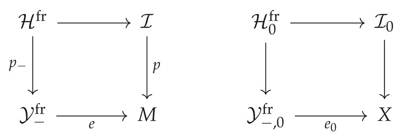 are Cartesian. The map $p_{-}$ is projective, ${\mathcal{H}}^{\mathrm{fr}}$ is smooth, and ${\mathcal{H}}_0^{\mathrm{fr}}$ is a reduced simple-normal-crossing union of smooth pullbacks ${\mathcal{H}}_{\ker }$ and ${\mathcal{H}}_{\mathrm{img}}$ meeting along ${\mathcal{Y}}_{-}^{\mathrm{fr}}{\times }_{M}Z$. The invariant line varies over ${\mathbb{P}}^1$. 

Proof. 

These are the defining fiber products. Projectivity of $p_{-}$ follows from that of  p . Smoothness of  e  implies smoothness of ${\mathcal{H}}^{\mathrm{fr}}\to \mathcal{I}$ and ${\mathcal{H}}_0^{\mathrm{fr}}\to {\mathcal{I}}_0$. The transverse local equations $\alpha \delta =0$ and the identification of the overlap therefore persist under smooth pullback. □

Write $I_X^H:={\mathrm{IC}}_X^H$, $R_X^H:=i_{o*}{\mathbb{Q}}_{\left\{o\right\}}^H(-2)$, and let ${ϵ}_X:R_X^H\to I_X^H\left[1\right]$ be the chosen nonzero local forward generator normalized in Section 2.2. Put $T:=e_0^{-1}\left(o\right)$ and denote its inclusion by $i_T:T\hookrightarrow {\mathcal{Y}}_{-,0}^{\mathrm{fr}}$.

Proposition 25

(Extension survival through evaluation and incidence pullback).  Assume $B^{\circ }\ne ⌀$. The normalized smooth pullback 

$${ϵ}_{\mathrm{ev}}:=e_0^{*}{ϵ}_X\left[r\right]:e_0^{*}{R}_X^H\left[r\right]⟶e_0^{*}{I}_X^H[r+1]$$

(84)

 is nonzero, with both endpoints in $\mathrm{MHM}\left({\mathcal{Y}}_{-,0}^{\mathrm{fr}}\right)$. Its pullback along the kernel-line incidence projection $p_{-,\ker }:{\mathcal{H}}_{\ker }\to {\mathcal{Y}}_{-,0}^{\mathrm{fr}}$ is also nonzero; the transverse component is the codimension-two Gysin morphism of Proposition 31, up to the original nonzero rational normalization. 

Proof. 

Smooth base change for the Cartesian square determined by $i_o$ and $i_T$ gives a natural isomorphism $i_T^{!}{e}_0^{*}\simeq e_T^{*}{i}_o^{!}$, where $e_T:T\to \left\{o\right\}$ is the structure map. Since ${ϵ}_X$ corresponds by closed-point adjunction to a nonzero scalar in ${\mathrm{End}}_{{\mathrm{MHS}}_{\mathbb{Q}}}\left({\mathbb{Q}}^H(-2)\right)$, the extraordinary restriction of ${ϵ}_{\mathrm{ev}}$ contains its pullback along $e_T$, with the common shift $\left[r\right]$. Pullback to the nonempty smooth  T  takes that scalar to the same nonzero endomorphism of ${\mathbb{Q}}_T^H\left[r\right](-2)$; equivalently, the induced map of the associated constant rank-one local systems is injective on this scalar Hom line. Hence ${ϵ}_{\mathrm{ev}}\ne 0$.

The base change of $p_{-,\ker }$ by a local smooth chart of  e  is the product of $m_{\ker }:D_{\ker }\to X$ with a smooth factor. Proposition 31 identifies $m_{\ker }^{*}{ϵ}_X$ with a nonzero purity-normalized Gysin component. Smooth external product preserves its nonzero Thom class. Restricting the full incidence pullback to this kernel branch also proves nonvanishing before any target pushforward. □

Proposition 26

(Geometric map to the modified-Higgs stack).  Let ${\mathfrak{H}}_{2,d-1}$ denote the stack of rank-two Higgs bundles of degree $d-1$, where $d=\mathrm{deg}{E}_{-}$. The elementary modification defines 

$$q_{+}:{\mathcal{H}}^{\mathrm{fr}}⟶{\mathfrak{H}}_{2,d-1},(E_{-},{\theta }_{-},\ell )⟼(E_{+},{\theta }_{+}),$$

(85)

 where $E_{+}:=\ker (E_{-}\to {\left(E_{-}\right)}_z/\ell )$ and ${\theta }_{+}:={\theta }_{-}{|}_{E_{+}}$. One has $\det {\theta }_{+}\left(z\right)=\det {\theta }_{-}\left(z\right)$, so restriction to the determinant-zero locus is Cartesian with the corresponding closed target substack. No properness assertion for $q_{+}$ is made. 

Proof. 

The universal length-one quotient is flat over the incidence parameter space and has a locally free elementary kernel. Invariance of  ℓ  makes the restricted Higgs field regular by (74). Proposition 10 makes this construction independent of adapted frames. Conjugation on the punctured formal disk preserves the characteristic polynomial, and regularity extends this equality to  z ; the determinant restriction is therefore a fiber-product equation. □

Lemma 13

(Intrinsic modified fiber and distinguished target line).  Let $S:=\ell \subset {\left(E_{-}\right)}_z$ and $Q:={\left(E_{-}\right)}_z/S$. The modified fiber $F_z:={\left(E_{+}\right)}_z$ has a functorial exact sequence 

$$0⟶Q\otimes K_z⟶F_z⟶S⟶0.$$

(86)

 The target distinguished line ${\ell }_{+}:=\ker (F_z\to {\left(E_{-}\right)}_z)$ is canonically $Q\otimes K_z$. These constructions commute with families of invariant lines. 

Proof. 

Tensor $0\to E_{+}\to E_{-}\to Q\otimes {\mathcal{O}}_z\to 0$ with ${\mathcal{O}}_z$. The Tor term is ${\mathrm{Tor}}_1^{{\mathcal{O}}_C}(Q\otimes {\mathcal{O}}_z,{\mathcal{O}}_z)\simeq Q\otimes {\mathfrak{m}}_z/{\mathfrak{m}}_z^2=Q\otimes K_z$, while the image of $F_z\to {\left(E_{-}\right)}_z$ is  S . In an adapted frame the Tor generator is the class of $w{e}_2$ in $E_{+}/w{E}_{+}$, giving the asserted distinguished line. The universal quotient and its Tor sequence are compatible with base change along the projective line of choices of  S . □

Proposition 27

(Hecke exchange of marked determinantal branches).  Let ${\alpha }_{-},{\delta }_{-}\in K_z$ be the eigenvalues of ${\theta }_{-}\left(z\right)$ on S and ${\left(E_{-}\right)}_z/S$, and let ${\alpha }_{+},{\delta }_{+}$ be the eigenvalues of ${\theta }_{+}\left(z\right)$ on ${\ell }_{+}$ and $F_z/{\ell }_{+}$, respectively. Then 

$${\alpha }_{+}={\delta }_{-},{\delta }_{+}={\alpha }_{-}.$$

(87)

 Thus the marked source kernel-line equation ${\alpha }_{-}=0$ becomes the target image-line equation ${\delta }_{+}=0$, and the source image-line equation ${\delta }_{-}=0$ becomes the target kernel-line equation ${\alpha }_{+}=0$. Their common intersection maps into the marked-target nilpotent incidence locus. 

Proof. 

In an adapted frame $A_0=\left(\begin{array}{cc}{a}_0& b_0\\ 0& d_0\end{array}\right)$ acts by $a_0$ on  S  and by $d_0$ on  Q . The induced matrix in the modified frame $(e_1,w{e}_2)$ is $A_{+}\left(0\right)=\left(\begin{array}{cc}{a}_0& 0\\ c_1& d_0\end{array}\right)$, and ${\ell }_{+}$ is the  second  basis line. The target eigenvalues on ${\ell }_{+}$ and its quotient are therefore $d_0$ and $a_0$. The assertions follow, independently of the adapted frame, by Lemma 13. For ${\alpha }_{+}=0$ the target matrix kills ${\ell }_{+}$; for ${\delta }_{+}=0$ its image lies in ${\ell }_{+}$. Both conditions hold on the source overlap. □

Lemma 14

(Node locus in the modified-Higgs evaluation).  On the source-node locus $T=e^{-1}\left(o\right)$ and the affine line chart $\ell =\mathbb{C}(e_1+\lambda e_2)$, one has 

$$A_{+}\left(0\right)=\left(\begin{array}{cc}0& 0\\ {\gamma }_1\left(\lambda \right)& 0\end{array}\right),{\gamma }_1\left(\lambda \right)=c_1+(d_1-a_1)\lambda -b_1{\lambda }^2.$$

(88)

 The modified value is regular nilpotent for ${\gamma }_1\left(\lambda \right)\ne 0$ and zero otherwise. Above a fixed source-node point all lines are allowed, giving the full ${\mathbb{P}}^1$ incidence fiber. 

Proof. 

When $A_0=0$, the lower-left entry of the moving adapted matrix $B_{\lambda }^{-1}A\left(w\right)B_{\lambda }$ is $w{\gamma }_1\left(\lambda \right)+O\left(w^2\right)$. Conjugation by $D=\mathrm{diag}(1,w)$ gives the formula. Its rank proves the stated nilpotent alternatives. □

Proposition 28

(Intrinsic first-jet quadratic and root configurations).  Suppose ${\theta }_{-}\left(z\right)=0$. Its first jet is an intrinsic tensor $J_1\left({\theta }_{-}\right)\in \mathrm{End}\left({\left(E_{-}\right)}_z\right)\otimes K_z^{\otimes 2}$. Over $E=\mathbb{P}\left({\left(E_{-}\right)}_z\right)$, let $\mathcal{S}={\mathcal{O}}_E(-1)$ and $\mathcal{Q}=({\left(E_{-}\right)}_z\otimes {\mathcal{O}}_E)/\mathcal{S}\simeq {\mathcal{O}}_E\left(1\right)$. The unique possibly nonzero component of ${\theta }_{+}\left(z\right)$ is the section 

$$\gamma \left(J_1\left({\theta }_{-}\right)\right)\in H^0\left(E,\mathrm{Hom}(\mathcal{S},\mathcal{Q})\otimes K_z^{\otimes 2}\right)\simeq H^0\left(E,{\mathcal{O}}_E\left(2\right)\otimes K_z^{\otimes 2}\right).$$

(89)

 Its zero scheme is the invariant-line scheme of $J_1\left({\theta }_{-}\right)$. This scheme is E if the first-jet endomorphism is scalar; it consists of two reduced points if its eigenvalues are distinct; and it is a nonreduced length-two point if it is nonscalar with a repeated eigenvalue. In particular, the third case includes nonzero nilpotent first jets. 

Proof. 

Since ${\theta }_{-}\left(z\right)=0$, taking its first derivative is independent of the connection and has value in ${(\mathrm{End}{E}_{-}\otimes K_C)}_z\otimes K_z=\mathrm{End}\left({\left(E_{-}\right)}_z\right)\otimes K_z^{\otimes 2}$. By Lemma 13, the source quotient  S  of $F_z$ and its distinguished subline $Q\otimes K_z$ give a component $S\to Q\otimes K_z^{\otimes 2}$. Its expression in the $\lambda$-chart is ${\gamma }_1\left(\lambda \right)$ of (88). On the other chart, with $\mu ={\lambda }^{-1}$, the corresponding polynomial is ${\gamma }_{\mu }=b_1+(a_1-d_1)\mu -c_1{\mu }^2=-{\mu }^2{\gamma }_1\left({\mu }^{-1}\right)$. This is precisely the transition rule for the section of $\mathrm{Hom}(\mathcal{S},\mathcal{Q})\otimes K_z^{\otimes 2}$. Its vanishing is equivalent to $J_1\left({\theta }_{-}\right)S\subset S\otimes K_z^{\otimes 2}$. The discriminant ${(a_1-d_1)}^2+4b_1{c}_1$ gives the three scheme-theoretic possibilities, as in Lemma 7. □

Remark 19

(Geometric meaning and remaining target calculation).  The branch exchange (87) concerns marked source and target lines, not an Atiyah flop between fixed resolutions. The nonempty rank-one target image provided by Corollary 3 is the geometric locus on which Theorem 8 proves nonvanishing of both genuine derived target images for the selected unit kernel and equivariant coefficient. This result does not compute all target perverse attachments, arbitrary-kernel transport, or the realization of an unrelated nodal $X_0$. 

5. Local Transport Benchmarks and Information Loss

We calculate the image of the corrected forward conifold extension under the kernel-line small resolution and its projection to the line parameter space. The extension is represented, after pullback, by a codimension-two Gysin morphism along the exceptional curve. Fiber contraction then identifies ordinary pushforward with restriction to the zero section and exceptional pushforward with extraordinary restriction. This explains, at the level of actual morphisms, why one operation annihilates the extension while the other preserves it. The Thom and derived-Hom calculations determine both transported arrows, their perverse degrees, and the boundary residual. We also record the perverse degree of $p_0^{*}{\mathrm{IC}}_X^H$ on the  full  normal-crossing incidence space, which is needed for the possible finite-target degree-two derived refinement. A compact octahedral check keeps the composition boundary separate from the forward Yoneda arrow. The auxiliary target here is ${\mathbb{P}}^1$, not the genuine modified-Higgs stack; over the latter, localized unit-kernel survival is proved in Theorem 8.

5.1. The Kernel-Line Correspondence

We use Section 1.6. Put $V={\mathbb{C}}^2$, $E=\mathbb{P}\left(V\right)$, $X=\{A\in \mathrm{End}(V):\det A=0\}$, and $o=0$. The kernel-line resolution (Proposition 16) is

$$X\stackrel{m}{\leftarrow }\tilde{X}\stackrel{q}{\to }E,\tilde{X}=\{(A,\ell ):A\ell =0\}\simeq {\mathrm{Tot}}_E\left({\mathcal{O}}_E{(-1)}^{\oplus 2}\right).$$

(90)

Let $k:E\hookrightarrow \tilde{X}$ be the zero section, $i_o:\left\{o\right\}\hookrightarrow X$, and $j:\tilde{X}\setminus E\hookrightarrow \tilde{X}$ the complement. Then $m\circ k=i_o$ and $q\circ k={\mathrm{id}}_E$. We take the nonzero corrected local class $ϵ$ of [7]:

$$I^H⟶P^H⟶R^H\stackrel{ϵ}{\to }{I}^H\left[1\right],I^H={\mathrm{IC}}_X^H,R^H=i_{o*}{\mathbb{Q}}_{\left\{o\right\}}^H(-2).$$

(91)

All pullbacks below are derived; in particular $m^{*}$ is not perverse  t -exact.

Proposition 29

(Pulled-back source coefficients).  Put 

$$K:={\mathbb{Q}}_{\tilde{X}}^H\left[3\right],L:=k_{*}{\mathbb{Q}}_E^H(-1)\left[1\right],T:=k_{*}{\mathbb{Q}}_E^H(-2)\left[1\right].$$

 There are identifications in $D^b\mathrm{MHM}\left(\tilde{X}\right)$ 

$$m^{*}{I}^H\simeq K\oplus L,m^{*}{R}^H\simeq T[-1].$$

(92)

 The three objects $K,L,T$ belong to $\mathrm{MHM}\left(\tilde{X}\right)$. The displayed splitting is compatible with the adjunction counit. 

Proof. 

By Corollary 2, $I^H\simeq R{m}_{*}K$. The counit $c:m^{*}{I}^H\to K$ is an isomorphism away from  E , and proper base change gives

$$i_o^{*}{I}^H\simeq R\mathsf{\Gamma }(E,{\mathbb{Q}}_E^H\left[3\right])\simeq {\mathbb{Q}}^H\left[3\right]\oplus {\mathbb{Q}}^H(-1)\left[1\right].$$

(93)

On restriction to  E , the map $k^{*}c$ projects onto ${\mathbb{Q}}_E^H\left[3\right]$; hence $\mathrm{Cone}\left(c\right)\simeq k_{*}{\mathbb{Q}}_E^H(-1)\left[2\right]=L\left[1\right]$. The connecting arrow in the triangle $L\to m^{*}{I}^H\to K\to L\left[1\right]$ vanishes, since

$${\mathrm{Hom}}_{D^b\mathrm{MHM}\left(E\right)}({\mathbb{Q}}_E^H\left[3\right],{\mathbb{Q}}_E^H(-1)\left[2\right])=0.$$

Thus the triangle splits compatibly with  c ; the corresponding splitting ambiguity also vanishes. The Cartesian inverse-image square for  m  and $i_o$ gives $m^{*}{R}^H\simeq k_{*}{\mathbb{Q}}_E^H(-2)=T[-1]$.

□

Proposition 30

(Perverse pullback on the full incidence central fiber).  Let $p_0:{\mathcal{I}}_0=D_{\ker }\cup D_{\mathrm{img}}\to X$ be the map of Proposition 19. Then 

$$A:=p_0^{*}{\mathrm{IC}}_X^H\in \mathrm{MHM}\left({\mathcal{I}}_0\right).$$

(94)

 The assertion is about the reducible union , not only its two smooth branches. 

Proof. 

Apply the natural Mayer–Vietoris restriction triangle to  A :

$$A⟶j_{\ker *}{A}_{\ker }\oplus j_{\mathrm{img}*}{A}_{\mathrm{img}}\stackrel{{\mathrm{res}}_{\ker }-{\mathrm{res}}_{\mathrm{img}}}{\to }{j}_{Z*}{A}_Z\stackrel{+1}{\to },$$

where $A_b=m_b^{*}{\mathrm{IC}}_X^H$ and $A_Z={\left(p_0{|}_Z\right)}^{*}{\mathrm{IC}}_X^H$. By Proposition 29, $A_b\simeq {\mathbb{Q}}_{D_b}^H\left[3\right]\oplus k_{b*}{\mathbb{Q}}_E^H(-1)\left[1\right]$; thus each $A_b$ is perverse. Restricting either counit-compatible branch splitting to  Z  gives

$$A_Z\simeq {\mathbb{Q}}_Z^H\left[3\right]\oplus k_{Z*}{\mathbb{Q}}_E^H(-1)\left[1\right].$$

Since  Z  is smooth of dimension two, the first summand has perverse degree $-1$ and the second degree 0. On perverse degree zero the signed difference of the two restriction maps is surjective: the exceptional-line summand of either $A_b$ restricts isomorphically onto the exceptional-line summand of $A_Z$. The long exact perverse cohomology sequence consequently has ${}^p{\mathcal{H}}^j\left(A\right)=0$ for $j\ne 0$. This calculation uses the  actual  restriction maps, not a formal direct-sum count of the endpoint objects. □

Corollary 4

(Perverse source degrees after smooth evaluation).  Let $e:{\mathcal{Y}}_{-}^{\mathrm{fr}}\to M$ be the smooth evaluation map of relative dimension r and put ${\mathcal{H}}_0^{\mathrm{fr}}={\mathcal{Y}}_{-}^{\mathrm{fr}}{\times }_M{\mathcal{I}}_0$. For the normalized incidence coefficients 

$$J_I:=p_{-,0}^{*}{e}_0^{*}{\mathrm{IC}}_X^H\left[r\right],J_R:=p_{-,0}^{*}{e}_0^{*}{i}_{o*}{\mathbb{Q}}^H(-2)\left[r\right],$$

 $J_I$ is perverse. Writing $D=T\times {\mathbb{P}}^1$ for the source-node inverse image and $i_D:D\hookrightarrow {\mathcal{H}}_0^{\mathrm{fr}}$, 

$$J_R\simeq i_{D*}{\mathbb{Q}}_D^H\left[r\right](-2)=\widehat{R}[-1],\widehat{R}:=i_{D*}{\mathbb{Q}}_D^H[r+1](-2)\in \mathrm{MHM}\left({\mathcal{H}}_0^{\mathrm{fr}}\right).$$

 Thus $J_R$ has perverse degree 1. These are source degrees; passage to a finite unframed target requires the separate correspondence and stack-normalization comparison. 

Proof. 

The projection ${\mathcal{H}}_0^{\mathrm{fr}}\to {\mathcal{I}}_0$ is the smooth base change of  e , so pullback shifted by $\left[r\right]$ is perverse  t -exact. The closed node inverse image  D  is smooth of dimension $r+1$, whence its constant Hodge module becomes perverse after the shift $[r+1]$. This gives both assertions without a claim of target perverse concentration. □

Lemma 15

(Zero-section contraction on the benchmark coefficients).  For F in the full triangulated subcategory of $D^b\mathrm{MHM}\left(\tilde{X}\right)$ generated by $K,L,T$, the natural comparison morphisms 

$$R{q}_{*}F⟶k^{*}F,k^{!}F⟶R{q}_{!}F$$

 are isomorphisms. In particular, they apply to $m^{*}{I}^H$, $m^{*}{R}^H$, $m^{*}{P}^H$ and their connecting morphisms. 

Proof. 

The first comparison is induced by the unit $F\to k_{*}{k}^{*}F$, followed by $R{q}_{*}$; the second by the counit $k_{*}{k}^{!}F\to F$, followed by $R{q}_{!}$ and $qk={\mathrm{id}}_E$. For $K={\mathbb{Q}}_{\tilde{X}}^H\left[3\right]$, both maps are the standard vector-bundle homotopy and compact-support Thom isomorphisms:

$$R{q}_{*}K\simeq k^{*}K\simeq {\mathbb{Q}}_E^H\left[3\right],k^{!}K\simeq R{q}_{!}K\simeq {\mathbb{Q}}_E^H(-2)[-1].$$

For  L  and  T , which are supported on the zero section, $k^{*}{k}_{*}\simeq k^{!}{k}_{*}\simeq \mathrm{id}$ and both pushforwards along $qk$ are the identity. The comparison transformations are natural transformations of exact derived functors. Their cones vanish on the three generators, hence on the triangulated subcategory they generate. Finally $m^{*}{P}^H$ belongs to this subcategory by (91) and (92). □

5.2. Local Gysin Representatives of the Extension

Lemma 16

(The forward Ext line).  Closed-point adjunction and the ODP costalk calculation give the one-dimensional forward extension space 

$${\mathrm{Ext}}_{\mathrm{MHM}\left(X\right)}^1(R^H,I^H)\simeq {\mathrm{End}}_{{\mathrm{MHS}}_{\mathbb{Q}}}\left({\mathbb{Q}}^H(-2)\right)\simeq \mathbb{Q}.$$

(95)

 Here $R^H$ is the quotient, not the subobject. 

Proof. 

Adjunction identifies the left side with ${\mathrm{Hom}}_{D^b{\mathrm{MHS}}_{\mathbb{Q}}}({\mathbb{Q}}^H(-2),i_o^{!}{I}^H\left[1\right])$. Lemma 2 gives ${\mathcal{H}}^1\left(i_o^{!}{I}^H\right)={\mathbb{Q}}^H(-2)$ and no lower costalk cohomology. Truncation reduces the derived Hom to the endomorphism group displayed in (95).

□

Proposition 31

(Geometric representative of the pulled-back class).  Let $g_E:k_{*}{\mathbb{Q}}_E^H(-2)\to K\left[1\right]$ be the codimension-two Gysin morphism, defined by the purity adjunction map for k. Relative to (92), one has 

$$m^{*}ϵ=(\gamma g_E,0):k_{*}{\mathbb{Q}}_E^H(-2)⟶K\left[1\right]\oplus L\left[1\right],\gamma \in {\mathbb{Q}}^{\times }.$$

(96)

 In particular, $m^{*}ϵ\ne 0$. The scalar γ records the normalization of the imported source generator; it is not set equal to 1 without choosing that normalization. 

Proof. 

Since  k  is a codimension-two regular immersion, $k^{!}{\mathbb{Q}}_{\tilde{X}}^H\left[4\right]\simeq {\mathbb{Q}}_E^H(-2)$. Purity and adjunction yield

$${\mathrm{Hom}}_{D^b\mathrm{MHM}\left(\tilde{X}\right)}(k_{*}{\mathbb{Q}}_E^H(-2),K\left[1\right])\simeq {\mathrm{End}}_{\mathrm{MHM}\left(E\right)}\left({\mathbb{Q}}_E^H(-2)\right)\simeq \mathbb{Q}.$$

(97)

The identity corresponds to $g_E$. Let $c:m^{*}{I}^H\to K$ be the counit used in Proposition 29. Then $c\left[1\right]m^{*}ϵ=\gamma g_E$. The unit $\eta :\mathrm{id}\to R{m}_{*}{m}^{*}$ and the triangular identity give

$$R{m}_{*}\left(c\left[1\right]m^{*}ϵ\right){\eta }_{R^H}=ϵ,$$

so $\gamma \ne 0$. For the other summand, the square $m\circ k=i_o$ identifies $k^{*}{m}^{*}ϵ$ with the pullback of $i_o^{*}ϵ:{\mathbb{Q}}^H(-2)\to {\mathbb{Q}}^H\left[4\right]\oplus {\mathbb{Q}}^H(-1)\left[2\right]$. This arrow vanishes since rational mixed Hodge structures have cohomological dimension one, so the indicated higher Ext groups vanish. The second summand of $m^{*}ϵ$ has both ends in the essential image of the fully faithful $k_{*}$, and therefore vanishes. This proves (96).

□

Proposition 32

(Reconstruction of the pulled-back middle coefficient).  Let $j:\tilde{X}\setminus E\hookrightarrow \tilde{X}$ be as above. For a nonzero forward class ϵ, the pulled-back middle coefficient admits an isomorphism 

$$m^{*}{P}^H\simeq R{j}_{*}{\mathbb{Q}}_{\tilde{X}\setminus E}^H\left[3\right]\oplus k_{*}{\mathbb{Q}}_E^H(-1)\left[1\right].$$

(98)

 The first summand contains the nontrivial Postnikov attachment induced by the Gysin morphism; the two perverse cohomology objects of $m^{*}{P}^H$ alone do not determine it. 

Proof. 

Rotate the pulled-back triangle to $k_{*}{\mathbb{Q}}_E^H(-2)[-1]\stackrel{(\gamma g_E[-1],0)}{\to }K\oplus L\to m^{*}{P}^H\to$. For the open complement  j , purity identifies the first map in the localization triangle $k_{*}{k}^{!}K\to K\to R{j}_{*}{j}^{*}K\to$ with $g_E[-1]$, and $k_{*}{k}^{!}K\simeq k_{*}{\mathbb{Q}}_E^H(-2)[-1]$. Rescaling this arrow by $\gamma \in {\mathbb{Q}}^{\times }$ leaves its cone unchanged. The direct sum with the zero map to  L  therefore yields $m^{*}{P}^H\simeq R{j}_{*}{j}^{*}K\oplus L$ as stated.

□

Remark 20

(Degree and realization).  The source ϵ is a Yoneda ${\mathrm{Ext}}^1$ class, whereas $m^{*}ϵ:T[-1]\to (K\oplus L)\left[1\right]$ belongs to ${\mathrm{Ext}}_{\mathrm{MHM}\left(\tilde{X}\right)}^2(T,K\oplus L)$. Its nonzero component is the purity-normalized Gysin map with Tate twist $(-2)$; it is not determined by the perverse graded objects. 

5.3. Ordinary Versus Compactly Supported Pushforward

Proposition 33

(Explicit transport of the three coefficients).  Let $q:\tilde{X}\to E$ be the rank-two vector-bundle projection. In $D^b\mathrm{MHM}\left(E\right)$ one has 

$$\begin{array}{cccc}\hfill R{q}_{*}{m}^{*}{I}^H& \simeq {\mathbb{Q}}_E^H\left[3\right]\oplus {\mathbb{Q}}_E^H(-1)\left[1\right],\hfill & \hfill R{q}_{!}{m}^{*}{I}^H& \simeq {\mathbb{Q}}_E^H(-2)[-1]\oplus {\mathbb{Q}}_E^H(-1)\left[1\right],\hfill \end{array}$$

(99)

$$\begin{array}{cccc}\hfill R{q}_{*}{m}^{*}{R}^H& \simeq {\mathbb{Q}}_E^H(-2),\hfill & \hfill R{q}_{!}{m}^{*}{R}^H& \simeq {\mathbb{Q}}_E^H(-2).\hfill \end{array}$$

(100)

 Under the splittings in (99), the actual transported connecting arrows are 

$$R{q}_{*}{m}^{*}ϵ=0,R{q}_{!}{m}^{*}ϵ=(\gamma \mathrm{id},0)\ne 0.$$

(101)

 Consequently 

$$\begin{array}{cc}\hfill R{q}_{*}{m}^{*}{P}^H& \simeq {\mathbb{Q}}_E^H\left[3\right]\oplus {\mathbb{Q}}_E^H(-1)\left[1\right]\oplus {\mathbb{Q}}_E^H(-2),\hfill \end{array}$$

(102)

$$\begin{array}{cc}\hfill R{q}_{!}{m}^{*}{P}^H& \simeq {\mathbb{Q}}_E^H(-1)\left[1\right].\hfill \end{array}$$

(103)

 The isomorphisms of the middle objects are compatible with the transported triangles; a choice of splitting of the zero connecting morphism is not asserted to be intrinsic. 

Proof. 

The rank-two vector-bundle homotopy and Thom isomorphisms give

$$\begin{array}{cc}\hfill R{q}_{*}{\mathbb{Q}}_{\tilde{X}}^H& \simeq {\mathbb{Q}}_E^H,\hfill \\ \hfill R{q}_{!}{\mathbb{Q}}_{\tilde{X}}^H& \simeq {\mathbb{Q}}_E^H(-2)[-4].\hfill \end{array}$$

Since $qk={\mathrm{id}}_E$ and  k  is proper, applying these identities to (92) gives (99)–(100).

For the connecting arrow, Lemma 15 identifies its ordinary image with $k^{*}{m}^{*}ϵ$. The proof of Proposition 31 calculates this restriction to be zero. Its extraordinary image is identified with $k^{!}{m}^{*}ϵ$; by purity, the adjoint of $g_E$ restricts to ${\mathrm{id}}_{{\mathbb{Q}}_E^H(-2)}$. This proves (101).

For an independent Hom check, $R{q}_{*}{g}_E$ belongs to ${\mathrm{Hom}}_{D^b\mathrm{MHM}\left(E\right)}({\mathbb{Q}}_E^H(-2),{\mathbb{Q}}_E^H\left[4\right])$. Using $R\mathsf{\Gamma }(E,{\mathbb{Q}}_E^H)\simeq {\mathbb{Q}}^H\oplus {\mathbb{Q}}^H(-1)[-2]$, this group is

$${\mathrm{Ext}}_{{\mathrm{MHS}}_{\mathbb{Q}}}^4(\mathbb{Q}(-2),\mathbb{Q})\oplus {\mathrm{Ext}}_{{\mathrm{MHS}}_{\mathbb{Q}}}^2(\mathbb{Q}(-2),\mathbb{Q}(-1))=0.$$

The !-image of $g_E$ is independently the Thom identity by fiber integration. Applying the two exact pushforward functors to (91), the zero ordinary connecting arrow gives the split middle object (102); the !-arrow cancels an isomorphic summand and yields (103).

□

Corollary 5

(Perverse cohomology of the benchmark).  Let $S_E:={\mathbb{Q}}_E^H\left[1\right]\in \mathrm{MHM}\left(E\right)$. The nonzero perverse cohomology objects of the transported coefficients are as follows: 

$$\begin{array}{cc}\mathrm{Object}& \mathrm{Nonzero}{}^p{\mathcal{H}}^n\hfill \\ R{q}_{!}{m}^{*}{I}^H& {}^p{\mathcal{H}}^0=S_E(-1),{}^p{\mathcal{H}}^2=S_E(-2)\hfill \\ R{q}_{*}{m}^{*}{I}^H& {}^p{\mathcal{H}}^{-2}=S_E,{}^p{\mathcal{H}}^0=S_E(-1)\hfill \\ R{q}_{!}{m}^{*}{R}^H=R{q}_{*}{m}^{*}{R}^H& {}^p{\mathcal{H}}^1=S_E(-2)\hfill \\ R{q}_{!}{m}^{*}{P}^H& {}^p{\mathcal{H}}^0=S_E(-1)\hfill \\ R{q}_{*}{m}^{*}{P}^H& {}^p{\mathcal{H}}^{-2}=S_E,{}^p{\mathcal{H}}^0=S_E(-1),{}^p{\mathcal{H}}^1=S_E(-2).\hfill \end{array}$$

 In particular, the compactly supported nonzero connecting arrow cancels the degree-one point-supported contribution; the ordinary image retains it. 

Proof. 

Each $S_E\left(a\right)\left[b\right]$ has its only nonzero perverse cohomology in degree $-b$. Thus ${\mathbb{Q}}_E^H\left[3\right]=S_E\left[2\right]$ contributes in degree $-2$, and ${\mathbb{Q}}_E^H(-2)[-1]=S_E(-2)[-2]$ in degree 2. Apply the same rule to the remaining summands of Proposition 33. The cancellation under $R{q}_{!}$ is the nonzero identity component of (101).

□

5.4. Boundary Residuals and Comparison Cones

Let $\mathcal{V}:={\mathcal{O}}_E{(-1)}^{\oplus 2}$. With the convention that ${\mathbb{P}}_E({\mathcal{O}}_E\oplus \mathcal{V})$ parameterizes lines, form

$$\overline{\tilde{X}}:={\mathbb{P}}_E({\mathcal{O}}_E\oplus \mathcal{V}),D_{\infty }:={\mathbb{P}}_E\left(\mathcal{V}\right).$$

The complement of $D_{\infty }$ is canonically $\tilde{X}={\mathrm{Tot}}_E\left(\mathcal{V}\right)$. Write

$$\iota :\tilde{X}\hookrightarrow \overline{\tilde{X}},d_{\infty }:D_{\infty }\hookrightarrow \overline{\tilde{X}},\overline{q}:\overline{\tilde{X}}\to E.$$

Then $\overline{q}$ is proper and $q=\overline{q}\circ \iota$.

Definition 17

(Boundary residual).  For $F\in D^b\mathrm{MHM}\left(\tilde{X}\right)$ define 

$${\mathrm{BRes}}_{D_{\infty }}\left(F\right):=\mathrm{Cone}\left({\iota }_{!}F⟶R{\iota }_{*}F\right)\in D^b\mathrm{MHM}\left(\overline{\tilde{X}}\right).$$

(104)

 It is supported on $D_{\infty }$ by recollement. The canonical map is the usual natural transformation ${\iota }_{!}\to R{\iota }_{*}$, not an arbitrarily chosen comparison. 

Proposition 34

(Boundary residual after proper projection).  For every $F\in D^b\mathrm{MHM}\left(\tilde{X}\right)$ there is a distinguished triangle 

$$R{q}_{!}F⟶R{q}_{*}F⟶R{\overline{q}}_{*}{\mathrm{BRes}}_{D_{\infty }}\left(F\right)\stackrel{+1}{\to }.$$

(105)

 For the pulled-back forward coefficient triangle, 

$$\begin{array}{cc}\hfill R{\overline{q}}_{*}{\mathrm{BRes}}_{D_{\infty }}\left(m^{*}{R}^H\right)& =0,\hfill \end{array}$$

(106)

$$\begin{array}{cc}\hfill R{\overline{q}}_{*}{\mathrm{BRes}}_{D_{\infty }}\left(m^{*}{I}^H\right)& \simeq {\mathbb{Q}}_E^H\left[3\right]\oplus {\mathbb{Q}}_E^H(-2),\hfill \end{array}$$

(107)

$$\begin{array}{cc}\hfill R{\overline{q}}_{*}{\mathrm{BRes}}_{D_{\infty }}\left(m^{*}{P}^H\right)& \simeq {\mathbb{Q}}_E^H\left[3\right]\oplus {\mathbb{Q}}_E^H(-2).\hfill \end{array}$$

(108)

 The map between the residuals of $m^{*}{I}^H$ and $m^{*}{P}^H$ induced by $a:I^H\to P^H$ is an isomorphism. 

Proof. 

Because $q=\overline{q}\iota$ and $\overline{q}$ is proper, applying $R{\overline{q}}_{*}$ to the defining cone yields (105). The object $m^{*}{R}^H=k_{*}{\mathbb{Q}}_E^H(-2)$ is supported away from $D_{\infty }$, so its residual is zero. For  K , the comparison $R{q}_{!}K\to R{q}_{*}K$ is zero: its Hom group is the group computed in the proof of Proposition 33. Its cone is ${\mathbb{Q}}_E^H\left[3\right]\oplus {\mathbb{Q}}_E^H(-2)$. For  L  the comparison is the identity, proving (107) via the counit-compatible splitting of (92). The natural transformation $R{q}_{!}\to R{q}_{*}$ gives a morphism of the two transported extension triangles. Its vertical cones form a distinguished triangle, and the quotient residual vanishes by (106); hence the map from the residual of $I^H$ to that of $P^H$ is an isomorphism. This gives (108) without choosing a splitting of the middle coefficient. It is the local boundary construction of [36].

□

5.5. Local Octahedral Validation

Definition 18

(Octahedral comparison defects).  For composable $u:A_0\to A_1$ and $v:A_1\to A_2$ in $D^b\mathrm{MHM}\left(E\right)$, write $D_u=\mathrm{Cone}\left(u\right)$, $D_v=\mathrm{Cone}\left(v\right)$, and $D_{vu}=\mathrm{Cone}(v\circ u)$. With the cohomological cone convention of Appendix C there is a triangle 

$$D_u⟶D_{vu}⟶D_v\stackrel{{\omega }_{u,v}}{\to }{D}_u\left[1\right].$$

(109)

 Its boundary ${\omega }_{u,v}$ is not the source forward Yoneda arrow. 

Proposition 35

(Split local octahedron).  Put $U={\mathbb{Q}}_E^H(-2)$, $L_1={\mathbb{Q}}_E^H(-1)\left[2\right]$, and $W_1={\mathbb{Q}}_E^H\left[4\right]$. For the maps furnished by the $R{q}_{!}\to R{q}_{*}$ comparison, 

$$U\stackrel{u=(\gamma \mathrm{id},0)}{\to }U\oplus L_1\stackrel{v=(0,\mathrm{id})}{\to }{W}_1\oplus L_1,$$

 $v\circ u=0$ and 

$$D_u\simeq L_1,D_{vu}\simeq W_1\oplus L_1\oplus U\left[1\right],D_v\simeq W_1\oplus U\left[1\right].$$

(110)

 The octahedral triangle splits, so ${\omega }_{u,v}=0$, even though $R{q}_{!}{m}^{*}ϵ\ne 0$. 

Proof. 

The comparison is identity on the zero-section-supported quotient and on $L_1$, and zero on the Thom summand mapping to $W_1$. Thus  u  is a split injection with complement $L_1$ and  v  projects onto $L_1$; their composite is zero. Taking the indicated cones gives (110) and a split octahedron. No conclusion about the original $ϵ$ follows from the vanishing of its different comparison boundary. □

Proposition 36

(The full $3\times 3$ comparison).  The two transported forward triangles and the natural map $R{q}_{!}\to R{q}_{*}$ yield a distinguished residual triangle 

$${\mathcal{B}}_I⟶{\mathcal{B}}_P⟶{\mathcal{B}}_R\stackrel{+1}{\to },$$

(111)

 where ${\mathcal{B}}_R=0$ and ${\mathcal{B}}_I\simeq {\mathcal{B}}_P\simeq W\oplus U$ with $W={\mathbb{Q}}_E^H\left[3\right]$ and $U={\mathbb{Q}}_E^H(-2)$. The first map is an isomorphism. 

Proof. 

Exactness gives a morphism of triangles; the stable $3\times 3$ lemma gives the residual triangle. Proposition 34 computes ${\mathcal{B}}_R=0$ and the other two residuals. A distinguished triangle ending in zero forces its first map to be an isomorphism. □

5.6. Limits of the Benchmark

Remark 21

(Scope of the computed transport).  Here q records the kernel line and has target $E\simeq {\mathbb{P}}^1$, not the modified-Higgs target $Y_{+}$ of (33). The $R{q}_{!}$ survival and $R{q}_{*}$ vanishing here express extraordinary versus ordinary detection on the exceptional locus; they are not results about the actual modified-Higgs target. On the latter, Theorem 8 proves nonvanishing for the selected unit kernel on the admissible rank-one open. 

Definition 19

(Verification requirements for the genuine transform).  For a geometric source realization $\mathsf{S}$ and Hecke kernel $\mathcal{K}$, the corresponding extension test consists of: 

(i)

 the actual Cartesian incidence and target diagrams, with their allowed base-change maps; 

(ii)

 the image of ϵ as a morphism, compared with the purity-normalized local Gysin representative; 

(iii)

 its perverse amplitude and Postnikov attachments on one target, preserving distinct ${\mathbb{Q}}^H(-1)$ and ${\mathbb{Q}}^H(-2)$ channels; 

(iv)

 the relevant !-to-* and framing-descent comparisons, including their residuals. 

 The source realization is available in Section 4.6. The actual target nonvanishing is known on the admissible rank-one open for the unit kernel (Theorem 8); other kernels, other strata, and unrestricted target perverse/Postnikov placement still require these tests. 

6. Derived Hecke Transport and MV–Octahedral Reconstruction

The evaluation-based incidence correspondence of Section 4.6 provides a geometric source realization of the universal determinantal conifold coefficient. We retain the varying invariant line, distinguish the resulting relative framed-value charts from their fixed-line fibers, and identify the Cartesian diagrams governing derived transport. The normalized pull–push functor carries the corrected forward triangle to a distinguished triangle, while its connecting morphism must be evaluated separately. We compute the point-supported quotient under both ordinary and exceptional direct images, including its perverse degrees and Tate twists on the varying-line chart. Recollement, MacPherson–Vilonen attaching equations, and geometric adjunction then constrain the remaining maps in the common target category. The octahedral construction is used only to check composition of specified maps, not as a substitute for an extension calculation. The final Hom/Ext ledger distinguishes three outcomes: the explicit nonproper affine-jet calculations; the localized nonvanishing of the unit-kernel forward morphism on the genuine rank-one modified-Higgs target (Theorem 8); and the finite rank-two inverse correspondence and its degree-two derived extension on a saturated open (Section 7.3); and the remaining global, arbitrary-kernel and off-open questions. We use the conventions of Section 1.6.

6.1. The Genuine Framed Correspondence Diagram

Let $V={\mathbb{C}}^2$, $X=\{A\in \mathrm{End}(V):\det A=0\}$, and $U_0=\left\{[1:\lambda ]\right\}\subset \mathbb{P}\left(V\right)$. The lower modification $E_{+}\subset E_{-}$ is that of Definition 6. The fixed-line calculation below is a closed fiber of the full varying-line incidence chart, used to check local shifts and twists.

Definition 20

(Fixed-line adapted fiber and varying-line chart).  For the fiber $\ell =\mathbb{C}{e}_1$, set $Y_{-}^{\mathrm{ad}}=\mathrm{Spec}\mathbb{C}[a_0,b_0,d_0]$, ${\mathcal{H}}^{\mathrm{ad},1}=\mathrm{Spec}\mathbb{C}[a_0,b_0,d_0,a_1,b_1,c_1,d_1]$, and $Y_{+}^{\mathrm{ad},0}=\mathrm{Spec}\mathbb{C}[a_0,d_0,c_1]$. The coordinate projections define 

$$Y_{-}^{\mathrm{ad}}\stackrel{p_{\mathrm{ad}}}{\leftarrow }{\mathcal{H}}^{\mathrm{ad},1}\stackrel{q_{\mathrm{ad}}}{\to }{Y}_{+}^{\mathrm{ad},0},$$

(112)

 where $p_{\mathrm{ad}}$ forgets $(a_1,b_1,c_1,d_1)$ and $q_{\mathrm{ad}}$ forgets $(b_0,a_1,b_1,d_1)$. Their matrices are $A_0=\left(\begin{array}{cc}{a}_0& b_0\\ 0& d_0\end{array}\right)$ and $A_{+}\left(0\right)=\left(\begin{array}{cc}{a}_0& 0\\ c_1& d_0\end{array}\right)$. 

 For the varying line ${\ell }_{\lambda }=\mathbb{C}(e_1+\lambda e_2)$, put $B_{\lambda }=\left(\begin{array}{cc}1& 0\\ \lambda & 1\end{array}\right)$. The actual affine chart of ${\mathcal{J}}_1^{\mathrm{inv}}$ over $U_0$ is 

$${\mathcal{H}}_{U_0}^{\mathrm{var},1}=\mathrm{Spec}\mathbb{C}[\lambda ,a_0,b_0,d_0,a_1,b_1,c_1,d_1].$$

 The coefficients are taken in the moving frame $B_{\lambda }$: $B_{\lambda }^{-1}{A}_0{B}_{\lambda }=\left(\begin{array}{cc}{a}_0& b_0\\ 0& d_0\end{array}\right)$. Define $Y_{-,U_0}^{\mathrm{var}}=U_0\times {\mathbb{A}}_{a_0,b_0,d_0}^3$ and $Y_{+,U_0}^{\mathrm{var},0}=U_0\times {\mathbb{A}}_{a_0,d_0,c_1}^3$. The projection $q_{U_0}$ retains λ and the value of the modified Higgs matrix in this moving adapted frame ; it is not the unframed Higgs-moduli projection $q_{+}$ of (85). 

Proposition 37

(Cartesian determinant restrictions and varying-line geometry).  The spaces in (112) have dimensions $3,7,3$; both projections are smooth, nonproper affine bundles of rank four. Define the fixed-line determinant loci $Y_{-,0}^{\mathrm{ad}}=V\left(a_0{d}_0\right)$, ${\mathcal{H}}_0^{\mathrm{ad},1}=V\left(a_0{d}_0\right)$, and $Y_{+,0}^{\mathrm{ad},0}=V\left(a_0{d}_0\right)$ in their respective ambient spaces. They form the restricted span 

$$Y_{-,0}^{\mathrm{ad}}\stackrel{p_0}{\leftarrow }{\mathcal{H}}_0^{\mathrm{ad},1}\stackrel{q_0}{\to }{Y}_{+,0}^{\mathrm{ad},0},$$

(113)

 with rank-four affine projections and a source map 

$$\rho :{\mathcal{H}}_0^{\mathrm{ad},1}⟶X,(A_0,A_1)⟼A_0.$$

(114)

 On the varying-line chart the maps are 

$$\begin{array}{cc}\hfill p_{U_0}(\lambda ,a_0,b_0,d_0,a_1,b_1,c_1,d_1)& =(\lambda ,a_0,b_0,d_0),\hfill \\ \hfill q_{U_0}(\lambda ,a_0,b_0,d_0,a_1,b_1,c_1,d_1)& =(\lambda ,a_0,d_0,c_1),\hfill \\ \hfill {\rho }_{U_0}(\lambda ,A_0,A_1)& =B_{\lambda }{A}_0{B}_{\lambda }^{-1}.\hfill \end{array}$$

 Both $p_{U_0}$ and $q_{U_0}$ are rank-four affine bundles. The determinant-zero restriction is Cartesian for either projection and is cut out by $a_0{d}_0=0$. The varying-line chart has dimension eight before this restriction, rather than seven. 

Proof. 

The independent coordinates exhibit each projection as forgetting four coordinates. In both frames $\det A_0=a_0{d}_0=\det A_{+}\left(0\right)$; hence the inverse images of the two determinant-zero loci are the same closed subscheme. The source map ${\rho }_{U_0}$ is regular because $B_{\lambda }$ and $B_{\lambda }^{-1}$ have polynomial entries on $U_0$. Since every fiber of the projections is ${\mathbb{A}}^4$, neither is proper. The fixed-line expressions result by taking the closed fiber $\lambda =0$, not by choosing an open neighborhood of the whole line parameter space. □

Remark 22

(Framing changes and scope).  The analogous chart over $U_{\infty }$ and its transition functions are specified in Appendix A. The two charts glue at the level of modified lattices and induced frames; the scalars $(a_0,d_0,c_1)$ do not constitute global unframed coordinates. To determine the first jet of the modified field one must retain the second source jet. The fixed-line span (112) is a closed fiber of the incidence chart, not the genuine global Hecke correspondence. 

Definition 21

(Verified correspondence datum).  On the evaluation-regular locus of Section 4.6, let $e_0:{\mathcal{Y}}_{-,0}^{\mathrm{fr}}\to X$ be the smooth evaluation map, $p_{-,0}:{\mathcal{H}}_0^{\mathrm{fr}}\to {\mathcal{Y}}_{-,0}^{\mathrm{fr}}$ the proper incidence projection, and $q_{+,0}:{\mathcal{H}}_0^{\mathrm{fr}}\to {\mathfrak{H}}_{2,d-1,0}$ the restricted geometric Hecke map. The universal local coefficient is realized by ${\mathsf{S}}_{\mathrm{ev}}=e_0^{*}\left[r\right]$, with r the smooth relative dimension. Its pullback to the correspondence is $p_{-,0}^{*}{e}_0^{*}\left[r\right]$. For a derived target transform one additionally fixes a MHM category on the chosen finite-type target or quotient chart, a kernel ${\mathcal{K}}_H\in {\mathsf{D}}_H\left({\mathcal{H}}_0^{\mathrm{fr}}\right)$, a direct-image choice $\sigma \in \{*,!\}$, shifts and Tate twists, and boundedness assumptions. All base-change comparisons must be induced by the corresponding Cartesian diagrams of Proposition 24. For the unit kernel the quotient-stack rank-one comparison of Proposition 55 is additional geometric structure on a selected target open. Its costalk normalization is supplied by Lemma 23, and compatible framing comparisons are treated in Section 8. The framed source and unframed target have different groupoids: the the map from the framed atlas to the unframed Higgs target must not be treated as a finite morphism. On a smaller saturated rank-one open, the descended unframed correspondence is finite of degree two (Proposition 59); it is a different map from the composition with the frame torsor. For a global nodal $X_0$ unrelated to X, a separate source realization $\mathsf{S}:{\mathsf{D}}_H\left(X_0\right)\to {\mathsf{D}}_H\left(Y_{-}\right)$ is required. 

6.2. Definition of the Derived Transport Functor

Definition 22

(Correspondence transform).  For a verified datum as in Definition 21, with a map $s:Y_{-}\to X_0$ only when one is geometrically given, fix integers $d,m\in \mathbb{Z}$ and $\sigma \in \{*,!\}$. Define, on the specified bounded constructible domain, 

$${\mathsf{H}}_{{\mathcal{K}}_H}^{\sigma ,d,m}\left(F\right):=R{q}_{\sigma }\left(p^{*}{s}^{*}F\otimes {\mathcal{K}}_H\right)\left[d\right]\left(m\right),F\in {\mathsf{D}}_H\left(X_0\right).$$

(115)

 Here $R{q}_{*}=R{q}_{*}$ and $R{q}_{!}=R{q}_{!}$ denote the ordinary and exceptional derived direct images. The tensor factor ${\mathcal{K}}_H$ is independently specified. In the universal evaluation case $X_0=X$, the source realization is $e_0^{*}\left[r\right]$ and the actual expression is $R{q}_{+,0,\sigma }(p_{-,0}^{*}{e}_0^{*}F\otimes {\mathcal{K}}_H)[r+d]\left(m\right)$. Its target is the selected framed/unframed Higgs chart, not $Y_{+}^{\mathrm{ad},0}$. For arbitrary $X_0$, replace $s^{*}$ by the independently specified realization $\mathsf{S}$. 

Proposition 38

(Exact derived transport).  Assume that (115) is defined on the three terms and the arrows of the source triangle (19), and that all its operations preserve the specified bounded constructible categories. Then ${\mathsf{H}}_{{\mathcal{K}}_H}^{\sigma ,d,m}$ is exact as a functor of stable derived categories and carries the source triangle to 

$$\begin{array}{cc}\hfill \mathsf{H}\left(I^H\right)& ⟶\mathsf{H}\left(P^H\right)⟶\mathsf{H}\left(R_{\mathsf{\Sigma }}^H\right)\hfill \\ \hfill & \stackrel{\mathsf{H}\left({ϵ}_{\mathsf{\Sigma }}\right)}{\to }\mathsf{H}\left(I^H\right)\left[1\right],\hfill \end{array}$$

(116)

 where $\mathsf{H}={\mathsf{H}}_{{\mathcal{K}}_H}^{\sigma ,d,m}$. Exactness alone does not imply $\mathsf{H}\left({ϵ}_{\mathsf{\Sigma }}\right)\ne 0$ or perverse t-exactness. For the universal local coefficient and the unit kernel, a separate geometric argument establishes nonvanishing over the admissible rank-one target open in Theorem 8. 

Proof. 

Each operation in the verified pull–tensor–push construction is exact on the chosen stable category. Its composite preserves the source cofiber sequence and its connecting arrow, giving (116). Neither faithfulness on morphisms nor perverse  t -exactness follows. □

Definition 23

(Raw fixed-line jet transform).  On the fixed adapted determinant chart, let 

$$Y:=Y_{+,0}^{\mathrm{ad},0},\mathcal{H}:={\mathcal{H}}_0^{\mathrm{ad},1}.$$

 The algebraic source map $\rho :\mathcal{H}\to X$ and the affine-bundle map $q_0:\mathcal{H}\to Y$ are those of (114) and (113). With the unshifted derived constant Hodge complex ${\mathbb{Q}}_{\mathcal{H}}^H$ as tensor unit, put 

$${\mathsf{T}}_{\mathrm{ad},*}\left(F\right):=R{q}_{0*}{\rho }^{*}F,{\mathsf{T}}_{\mathrm{ad},!}\left(F\right):=R{q}_{0!}{\rho }^{*}F.$$

(117)

 These are the raw , unshifted and untwisted transport functors. Any later perverse normalization is displayed separately rather than absorbed into an unspecified convention. 

Lemma 17

(Unit-kernel normalization).  For the constant complex on the nodal conifold X one has 

$$\begin{array}{cc}\hfill {\mathsf{T}}_{\mathrm{ad},*}\left({\mathbb{Q}}_X^H\right)& \simeq {\mathbb{Q}}_Y^H,\hfill \\ \hfill {\mathsf{T}}_{\mathrm{ad},!}\left({\mathbb{Q}}_X^H\right)& \simeq {\mathbb{Q}}_Y^H(-4)[-8].\hfill \end{array}$$

(118)

 The isomorphisms arise from affine-bundle homotopy invariance and the rank-four Thom isomorphism, respectively. 

Proof. 

The inverse image of the constant derived Hodge complex is the constant derived Hodge complex, so ${\rho }^{*}{\mathbb{Q}}_X^H={\mathbb{Q}}_{\mathcal{H}}^H$. By Proposition 37, $q_0$ is a trivial affine bundle of complex rank four. Its ordinary pushforward sends the constant complex to the constant complex on  Y . Its exceptional pushforward is obtained from the compactly supported cohomology of ${\mathbb{A}}^4$, which is $\mathbb{Q}(-4)[-8]$. The algebraic orientation determines the indicated Tate twist. □

6.3. Reduction to a Common Terminal Category

Definition 24

(Typed comparison system).  Fix a finite-type target Y and a sequence of three derived MHM objects 

$$A_0,A_1,A_2\in {\mathsf{D}}_H\left(Y\right).$$

 A typed comparison system consists of specified morphisms 

$$A_0\stackrel{u}{\to }{A}_1\stackrel{v}{\to }{A}_2,$$

(119)

 with recorded geometric origin (adjunction, base change, specialization, or correspondence comparison). An equality of the isomorphism classes of $A_0,A_1,A_2$ does not supply either u or v. When the objects arise from the source extension, we use 

$$A_0=\mathsf{H}\left(I^H\right),A_1=\mathsf{H}\left(P^H\right),A_2=\mathsf{H}\left(R_{\mathsf{\Sigma }}^H\right),$$

(120)

 with $u=\mathsf{H}\left(a\right)$ and $v=\mathsf{H}\left(b\right)$; then $vu=0$ and the connecting morphism is $\mathsf{H}\left({ϵ}_{\mathsf{\Sigma }}\right)$. 

The actual universal-coefficient correspondence uses the following typed span, while the fixed-line model is its finite-jet fiber:

(121)

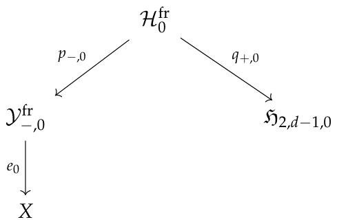
The first vertical map is smooth; the incidence projection is projective. The target projection is the geometric modified-Higgs map of Proposition 26, with neither global properness nor perverse  t -exactness presumed. On its kernel branch, after the compatible quotient-stack construction, it has the canonical inverse on the admissible rank-one target open of Proposition 55. This statement concerns the geometric branch and does not identify the affine-value target $Y_{+,U_0}^{\mathrm{var},0}$ with Higgs moduli.

Lemma 18

(Morphisms and their images).  For any two objects $F,G\in {\mathsf{D}}_H\left(X\right)$ and any morphism $\alpha :F\to G\left[n\right]\left(m\right)$, the local transform (117) induces a morphism 

$${\mathsf{T}}_{\mathrm{ad},\sigma }\left(\alpha \right):{\mathsf{T}}_{\mathrm{ad},\sigma }\left(F\right)⟶{\mathsf{T}}_{\mathrm{ad},\sigma }\left(G\right)\left[n\right]\left(m\right),\sigma \in \{*,!\}.$$

 For composable maps, ${\mathsf{T}}_{\mathrm{ad},\sigma }\left(\beta \alpha \right)={\mathsf{T}}_{\mathrm{ad},\sigma }\left(\beta \right){\mathsf{T}}_{\mathrm{ad},\sigma }\left(\alpha \right)$. 

Proof. 

Pullback, direct image, shift and Tate twist are functorial and commute with composition on the stated bounded domain. □

Remark 23

(Additional composable Hecke stages).  A sequence $A_0\to A_1\to A_2$ obtained from two modifications is defined only after the two correspondence spaces are related by a specified fiber product, the kernels are composed, and the resulting coefficients are pushed to one terminal space. This is the separate convolution problem of Section 9. In the present section (120) is the canonical composable system already supplied by the transported source extension. 

Proposition 39

(Two distinct target computations).  On the finite-dimensional adapted-value targets of (112), the morphisms $R{q}_{0*}{\rho }^{*}{ϵ}_X$ and $R{q}_{0!}{\rho }^{*}{ϵ}_X$ are not identified with the images of ${ϵ}_X$ under the geometric map $q_{+,0}$ of (121). For the latter, take the unit kernel, the descended quotient-stack normalization of Lemma 23, and the admissible rank-one open U of Proposition 55. When U meets the evaluated source-node locus in a regular-nilpotent point, the actual derived connecting arrow survives both $R{q}_{+,0*}$ and $R{q}_{+,0!}$ after restriction to U. The existence hypotheses for such a point are supplied by Corollary 7. 

Proof. 

The adapted-value target retains the moving-line coordinate and only a truncated Higgs value; its map $q_0$ is a nonproper affine bundle. The geometric $q_{+,0}$ instead changes the underlying bundle and has a quotient-stack target, so no Cartesian square identifying these pushforwards has been provided. For the second assertion use the canonical upper inverse on the rank-one target open together with the nonzero equivariant codimension-two Gysin class and closed-branch detection of Theorem 8. The first-jet existence corollary makes the stated open nonempty in its genus/determinant ranges. The stronger finite-open perverse calculation is proved separately in Theorem 9. □

6.4. Perverse Cohomological Amplitude

The raw affine-jet models compute direct images on  framed value spaces ; they are not perverse-normalized global Hecke functors. We begin with the fixed-line calculation and then retain the varying line as a target coordinate.

Proposition 40

(Node-supported quotient on the fixed-line fiber).  Let $R_o^H=i_{o*}{\mathbb{Q}}_{\left\{o\right\}}^H(-2)$ on X and $S=V(a_0,d_0)\subset Y=Y_{+,0}^{\mathrm{ad},0}$, so $S\simeq {\mathbb{A}}_{c_1}^1$; denote the inclusion by ${\iota }_S$. Then 

$$\begin{array}{cc}\hfill {\mathsf{T}}_{\mathrm{ad},*}\left(R_o^H\right)& \simeq {\iota }_{S*}{\mathbb{Q}}_S^H(-2),\hfill \\ \hfill {\mathsf{T}}_{\mathrm{ad},!}\left(R_o^H\right)& \simeq {\iota }_{S*}{\mathbb{Q}}_S^H(-5)[-6].\hfill \end{array}$$

(122)

 For $B_S={\iota }_{S*}{\mathbb{Q}}_S^H\left[1\right]\in \mathrm{MHM}\left(Y\right)$, their only nonzero perverse cohomology objects are 

$${}^p{\mathcal{H}}^1{\mathsf{T}}_{\mathrm{ad},*}\left(R_o^H\right)\simeq B_S(-2),{}^p{\mathcal{H}}^7{\mathsf{T}}_{\mathrm{ad},!}\left(R_o^H\right)\simeq B_S(-5).$$

(123)

 This is a calculation on $\lambda =0$ only. 

Proof. 

The inverse image of  o  under (114) has equations $a_0=b_0=d_0=0$, with coordinates $(a_1,b_1,c_1,d_1)$. Its map to  S  forgets $(a_1,b_1,d_1)$; it is therefore a rank-three affine bundle. The ordinary pushforward is constant on  S  and the exceptional pushforward has factor $\mathbb{Q}(-3)[-6]$. Including the source twist $(-2)$ proves (122). Since  S  is smooth of dimension one, ${\mathbb{Q}}_S^H\left[1\right]$ is perverse, giving the stated degrees. □

Proposition 41

(Node quotient with the invariant line unfrozen).  Let $Y_{U_0}:=V\left(a_0{d}_0\right)\subset Y_{+,U_0}^{\mathrm{var},0}$ and ${\mathcal{H}}_{U_0}:=V\left(a_0{d}_0\right)\subset {\mathcal{H}}_{U_0}^{\mathrm{var},1}$. Write ${\rho }_{U_0}:{\mathcal{H}}_{U_0}\to X$ and $q_{U_0}:{\mathcal{H}}_{U_0}\to Y_{U_0}$ for the maps above, and put $S_{U_0}=V(a_0,d_0)\subset Y_{U_0}$, with inclusion ${\iota }_{U_0}$. Thus $S_{U_0}\simeq U_0\times {\mathbb{A}}_{c_1}^1$ has complex dimension two. Define ${\mathsf{T}}_{U_0,\sigma }=R{q}_{U_0,\sigma }{\rho }_{U_0}^{*}$. Then 

$$\begin{array}{cc}\hfill {\mathsf{T}}_{U_0,*}\left(R_o^H\right)& \simeq {\iota }_{U_0*}{\mathbb{Q}}_{S_{U_0}}^H(-2),\hfill \\ \hfill {\mathsf{T}}_{U_0,!}\left(R_o^H\right)& \simeq {\iota }_{U_0*}{\mathbb{Q}}_{S_{U_0}}^H(-5)[-6].\hfill \end{array}$$

(124)

 With $B_{U_0}:={\iota }_{U_0*}{\mathbb{Q}}_{S_{U_0}}^H\left[2\right]$, 

$${}^p{\mathcal{H}}^2{\mathsf{T}}_{U_0,*}\left(R_o^H\right)\simeq B_{U_0}(-2),{}^p{\mathcal{H}}^8{\mathsf{T}}_{U_0,!}\left(R_o^H\right)\simeq B_{U_0}(-5).$$

(125)

 All other perverse degrees vanish on this chart. The change from (123) is an increase of one in perverse degree, not an additional Tate twist: λ remains a coordinate of the target. If it is subsequently integrated out by a nonproper projection, its compact-support cohomology must be evaluated for that separate map. 

Proof. 

For every $\lambda$, conjugation by $B_{\lambda }$ maps the zero matrix to itself. Hence ${\rho }_{U_0}^{-1}\left(o\right)=\{a_0=b_0=d_0=0\}\simeq U_0\times {\mathbb{A}}^4$. On this inverse image, $q_{U_0}$ has image $S_{U_0}$ and is the trivial affine bundle with fiber coordinates $(a_1,b_1,d_1)$. Homotopy invariance and the rank-three compact-support Thom isomorphism give the two lines of (124). Since $S_{U_0}$ has dimension two, the perverse-normalized constant object is ${\mathbb{Q}}_{S_{U_0}}^H\left[2\right]$. Rewriting the two terms as $B_{U_0}(-2)[-2]$ and $B_{U_0}(-5)[-8]$ proves (125). The construction is chartwise; globally the corresponding framed-value coordinates glue by the modified-frame transition functions of Appendix A, not by treating $c_1$ as an invariant function. □

Remark 24

(Perverse amplitude beyond the quotient).  Section 4.6 constructs the smooth evaluation realization and gives nonzero pullback of ${ϵ}_X$ to the incidence space. The calculations above determine the quotient object after raw local affine-jet pushforward, not the images of $I_X^H$, $P_X^H$, or their connecting morphism under the actual map $q_{+,0}$. Theorem 8 separately proves that the actual unit-kernel connecting morphism is nonzero after either target direct image on an admissible rank-one open. That conclusion is obtained by the inverse-branch/Gysin comparison, not from the affine-jet quotient formulas. A perverse placement theorem for the actual unframed unit-kernel transform on a smaller finite open $U^{\prime }$ uses, in addition, the full-incidence computation of Proposition 30 and the descent normalization; see Theorem 9. The raw affine-jet formulas alone do not establish that theorem or an arbitrary-kernel transform. 

Proposition 42

(Perverse cohomology of a transported triangle).  For a verified exact transform $\mathsf{H}$ with $I_Y=\mathsf{H}\left(I^H\right)$, $P_Y=\mathsf{H}\left(P^H\right)$ and $R_Y=\mathsf{H}\left(R_{\mathsf{\Sigma }}^H\right)$, there is a functorial long exact sequence 

$$\begin{array}{cc}\hfill \dots & \to {}^p{\mathcal{H}}^n\left(I_Y\right)\to {}^p{\mathcal{H}}^n\left(P_Y\right)\to {}^p{\mathcal{H}}^n\left(R_Y\right)\hfill \\ \hfill & \stackrel{{\partial }_n}{\to }{}^p{\mathcal{H}}^{n+1}\left(I_Y\right)\to {}^p{\mathcal{H}}^{n+1}\left(P_Y\right)\to \dots .\hfill \end{array}$$

(126)

 If $I_Y,R_Y\in \mathrm{MHM}\left(Y\right)$, then $P_Y\in \mathrm{MHM}\left(Y\right)$ and the triangle is a short exact sequence in that heart. Otherwise its derived Postnikov attachments remain part of the transport data. 

Proof. 

Apply the perverse cohomology functors to (116). The heart of a bounded  t -structure is extension closed; if both outer terms lie in that heart, so does the middle term and the sequence is short exact. □

6.5. MacPherson–Vilonen Attaching Data

Let $i:Z\hookrightarrow Y$ be a closed union of singular strata of the selected target and $j:U=Y\setminus Z\hookrightarrow Y$ its open complement. On the fixed-line chart $Z=S$; on the varying-line chart $Z=S_{U_0}$. For an object $M\in \mathrm{MHM}\left(Y\right)$, the primary recollement data are $j^{*}M$, $i^{*}M$, $i^{!}M$, together with their canonical connecting maps of Section 2.5.

Table 1. Raw affine-jet node-quotient images; $B_S={\iota }_{S*}{\mathbb{Q}}_S^H\left[1\right]$ and $B_{U_0}={\iota }_{U_0*}{\mathbb{Q}}_{S_{U_0}}^H\left[2\right]$. The unit-kernel derived survival theorem on the genuine target does not identify its perverse amplitude with these local quotient degrees.

Model	Ordinary $\mathit{R}{\mathit{q}}_{*}$	Exceptional $\mathit{R}{\mathit{q}}_{!}$
Fixed line	$n=1:B_S(-2)$	$n=7:B_S(-5)$
Varying line	$n=2:B_{U_0}(-2)$	$n=8:B_{U_0}(-5)$
$I^H$	Gysin/attaching map required	Gysin/attaching map required
$P^H$	determined by $\mathsf{T}\left(ϵ\right)$	determined by $\mathsf{T}\left(ϵ\right)$

Table 1. Raw affine-jet node-quotient images; $B_S={\iota }_{S*}{\mathbb{Q}}_S^H\left[1\right]$ and $B_{U_0}={\iota }_{U_0*}{\mathbb{Q}}_{S_{U_0}}^H\left[2\right]$. The unit-kernel derived survival theorem on the genuine target does not identify its perverse amplitude with these local quotient degrees.

Model	Ordinary $\mathit{R}{\mathit{q}}_{*}$	Exceptional $\mathit{R}{\mathit{q}}_{!}$
Fixed line	$n=1:B_S(-2)$	$n=7:B_S(-5)$
Varying line	$n=2:B_{U_0}(-2)$	$n=8:B_{U_0}(-5)$
$I^H$	Gysin/attaching map required	Gysin/attaching map required
$P^H$	determined by $\mathsf{T}\left(ϵ\right)$	determined by $\mathsf{T}\left(ϵ\right)$

Definition 25

(Kernel–cokernel attaching functors).  Let $A\in \mathrm{MHM}\left(U\right)$ and suppose the perverse cohomology objects below exist in the indicated bounded categories. Write 

$$J_{!}\left(A\right):={}^p{\mathcal{H}}^0\left(j_{!}A\right),J_{*}\left(A\right):={}^p{\mathcal{H}}^0\left(R{j}_{*}A\right),$$

 and let ${\nu }_A:J_{!}\left(A\right)\to J_{*}\left(A\right)$ be the canonical morphism. Its kernel and cokernel are supported on Z. Define $F\left(A\right),G\left(A\right)\in \mathrm{MHM}\left(Z\right)$ uniquely by 

$$i_{*}F\left(A\right)=\ker \left({\nu }_A\right),i_{*}G\left(A\right)=\mathrm{coker}\left({\nu }_A\right).$$

(127)

 A morphism $a:A\to A^{\prime }$ induces functorial maps $F\left(a\right)$ and $G\left(a\right)$. If a chosen MV presentation is expressed by data $(A,B,u,v)$ with $B\in \mathrm{MHM}\left(Z\right)$, $u:F\left(A\right)\to B$, and $v:B\to G\left(A\right)$, then a morphism $(a,b)$ of such data is required to satisfy 

$$b\circ u=u^{\prime }\circ F\left(a\right),G\left(a\right)\circ v=v^{\prime }\circ b.$$

(128)

 The equivalence between this presentation and the relevant subcategory of perverse Hodge modules is invoked only on strata where its hypotheses and the Hodge-module lifting data have been verified. 

Lemma 19

(Attaching constraints from a geometric comparison).  Let $h:M\to M^{\prime }$ be a morphism in $\mathrm{MHM}\left(Y\right)$, and denote by $a=j^{*}h$ its restriction to U and by $b=i^{*}h$ its restriction to Z in the appropriate derived sense. The naturality squares of the two recollement triangles commute. Whenever both objects admit the fixed MV description of Definition 25, their attached morphism $(a,b)$ satisfies (128). Conversely, an abstract solution of these equations determines a morphism of the chosen MV data, but need not determine a unique morphism of derived complexes outside the range of the specified gluing equivalence. 

Proof. 

The maps $j_{!}{j}^{*}M\to M$ and $M\to R{j}_{*}{j}^{*}M$ are respectively the adjunction counit and unit. Naturality of these transformations with respect to  h  produces a commutative diagram of the corresponding distinguished triangles. Applying perverse cohomology and taking kernels and cokernels of the canonical $J_{!}\to J_{*}$ morphism gives functoriality of  F  and  G . The maps to and from the closed-stratum coefficient must therefore satisfy the two equations in (128). The converse inside the chosen MV diagram category is the definition of a morphism of such diagrams; passage back to mixed Hodge modules requires the previously specified equivalence and does not follow from those equations alone. □

Proposition 43

(Closed-stratum data of the quotient image).  For the fixed-line quotient image of Proposition 40, one has 

$$j^{*}{}^p{\mathcal{H}}^1{\mathsf{T}}_{\mathrm{ad},*}\left(R_o^H\right)=0,i^{*}{}^p{\mathcal{H}}^1{\mathsf{T}}_{\mathrm{ad},*}\left(R_o^H\right)\simeq {\mathbb{Q}}_S^H\left[1\right](-2).$$

(129)

 The corresponding extraordinary restriction is isomorphic to the same closed-stratum object. For the exceptional transport, the analogous statement holds in perverse degree 7, with Tate type $(-5)$. Neither image has an open-stratum attaching component. 

Proof. 

Both complexes in (122) lie in the essential image of the closed pushforward $i_{*}$. Hence $j^{*}{i}_{*}=0$ while $i^{*}{i}_{*}\simeq i^{!}{i}_{*}\simeq \mathrm{id}$. Combining these identities with (123) proves each assertion. No nonzero attaching morphism from the intersection-complex side is inferred from the quotient alone. □

For the varying-line quotient, the analogous closed coefficient is $B_{U_0}(-2)$ in perverse degree 2, or $B_{U_0}(-5)$ in degree 8 for exceptional direct image. Both have zero open restriction.

For a positive-dimensional closed stratum, the residual extension information is retained in the recollement arrows $i^{!}M\to i^{*}M$ and $i^{*}M\to i^{*}R{j}_{*}{j}^{*}M$. A transverse normal slice may admit the classical nearby/vanishing-cycle zig-zag presentation, but it is not substituted for the relative gluing problem without an explicit equivalence [4,5,36]. On the admissible rank-one target open the  nonzero map  is already detected by the closed kernel branch; computing its full target recollement diagram and Postnikov attachments is a separate problem.

6.6. Adjunction and Octahedral Reconstruction

Definition 26

(Comparison cones).  For a typed system (119), set 

$$D_u:=\mathrm{Cone}\left(u\right),D_v:=\mathrm{Cone}\left(v\right),D_{vu}:=\mathrm{Cone}(v\circ u).$$

 Fix an enhanced derived category and compatible representatives of $u,v$, and $vu$ so that these cone objects and their comparison morphisms are defined coherently. 

Proposition 44

(Octahedral triangle and local long exact sequences).  The data of Definition 26 determine a distinguished triangle 

$$D_u⟶D_{vu}⟶D_v\stackrel{{\omega }_{u,v}}{\to }{D}_u\left[1\right].$$

(130)

 For every closed immersion $i:Z\hookrightarrow Y$ and every integer n, there are long exact sequences 

$$\begin{array}{cc}\hfill \dots & \to {\mathcal{H}}^n\left(i^{!}{D}_u\right)\to {\mathcal{H}}^n\left(i^{!}{D}_{vu}\right)\to {\mathcal{H}}^n\left(i^{!}{D}_v\right)\hfill \\ \hfill & \to {\mathcal{H}}^{n+1}\left(i^{!}{D}_u\right)\to \dots ,\hfill \end{array}$$

(131)

$$\begin{array}{cc}\hfill \dots & \to {\mathcal{H}}^n\left(i^{*}{D}_u\right)\to {\mathcal{H}}^n\left(i^{*}{D}_{vu}\right)\to {\mathcal{H}}^n\left(i^{*}{D}_v\right)\hfill \\ \hfill & \to {\mathcal{H}}^{n+1}\left(i^{*}{D}_u\right)\to \dots .\hfill \end{array}$$

(132)

 The natural transformation $i^{!}\to i^{*}$ induces a morphism from (131) to (132), compatible with every connecting arrow. 

Proof. 

The octahedral axiom applied to $A_0\stackrel{u}{\to }{A}_1\stackrel{v}{\to }{A}_2$ yields (130). In an enhanced setting the triangle is obtained by taking the cofibers of compatible chain-level representatives. Both $i^{!}$ and $i^{*}$ are exact derived functors, so applying them to the triangle gives distinguished triangles on  Z . Their cohomology long exact sequences are (131) and (132). Finally, the natural transformation $i^{!}\to i^{*}$ is functorial in its input. Applying it to the three morphisms of the octahedral triangle gives a morphism of triangles; naturality of connecting homomorphisms in a  t -structure proves compatibility of the two displayed long exact sequences. □

Lemma 20

(The extension octahedron and its Yoneda morphism).  For the particular coefficient triangle $A_0\stackrel{u}{\to }{A}_1\stackrel{v}{\to }{A}_2\stackrel{\epsilon }{\to }{A}_0\left[1\right]$ of (120), choose a strict chain model with $vu=0$. Then $D_u\simeq A_2$, $D_v\simeq A_0\left[1\right]$ and $D_{vu}\simeq A_2\oplus A_0\left[1\right]$. The resulting octahedral triangle is split, so its connecting morphism ${\omega }_{u,v}$ vanishes. This is a statement about the extension triangle , not about arbitrary composable maps with zero composite; it does not imply $\epsilon =\mathsf{H}\left({ϵ}_{\mathsf{\Sigma }}\right)=0$. 

Proof. 

The distinguished coefficient triangle identifies the first two cones with $A_2$ and $A_0\left[1\right]$. In the chain model of a short exact extension, $vu=0$ strictly. The cone of this zero composite is $A_2\oplus A_0\left[1\right]$; the octahedral maps are inclusion and projection under the induced identifications. Thus the connecting arrow is zero. The original $\epsilon$ occurs in the identification of the cones with the coefficient triangle; it is not the octahedral boundary. An arbitrary pair $u,v$ with $vu=0$ need not give a split octahedron. □

Remark 25

(Comparison with convolution).  An octahedron of three coefficient morphisms is not a convolution theorem for two Hecke kernels. The latter requires a geometric composition of correspondences and a natural comparison of the corresponding push–pull functors, including the kernel convolution and its associativity data. The first construction is used here for derived reconstruction. The second is addressed in Section 9, with the specialization input of [24,25,28]. 

6.7. Uniqueness and Hom/Ext Ambiguities

Proposition 45

(Linear constraints on closed-stratum liftings).  Fix two MV diagrams $(A,B,u,v)$ and $(A^{\prime },B^{\prime },u^{\prime },v^{\prime })$. Let $a:A\to A^{\prime }$ be a fixed open-stratum morphism. Suppose $b_0:B\to B^{\prime }$ satisfies (128). The solutions b form the affine subspace 

$$b_0+\ker \left(\begin{array}{cc}\hfill {\mathrm{Hom}}_{\mathrm{MHM}\left(Z\right)}(B,B^{\prime })& ⟶{\mathrm{Hom}}_{\mathrm{MHM}\left(Z\right)}(F\left(A\right),B^{\prime })\hfill \\ \hfill & \oplus {\mathrm{Hom}}_{\mathrm{MHM}\left(Z\right)}(B,G\left(A^{\prime }\right)),\hfill \\ \hfill \delta & ⟼(\delta u,v^{\prime }\delta )\hfill \end{array}\right).$$

(133)

 In particular, if this kernel is zero, b is unique within the fixed MV presentation. Existence and uniqueness of a derived lift require additional control of the corresponding higher Hom/Ext groups and of any chosen enhancement. 

Proof. 

Suppose  b  and $b_0$ satisfy the two equations of (128) for the same  a . Subtracting gives $(b-b_0)u=0$ and $v^{\prime }(b-b_0)=0$. Thus $\delta =b-b_0$ lies in the indicated kernel. Conversely, if $\delta$ lies in that kernel, then $(b_0+\delta )u=b_{0}u=u^{\prime }F\left(a\right)$ and $v^{\prime }(b_0+\delta )=v^{\prime }{b}_0=G\left(a\right)v$. Hence $b_0+\delta$ is another solution, giving the claimed affine description. The assertion is internal to the fixed MV diagram category; no fullness or uniqueness of a realization functor on derived morphisms has been used. □

Lemma 21

(Pure Tate Hom constraints on the node line).  Let $S\simeq {\mathbb{A}}^1$ be the stratum of Proposition 40. Then 

$$\begin{array}{cc}\hfill {\mathrm{Hom}}_{\mathrm{MHM}\left(S\right)}({\mathbb{Q}}_S^H\left[1\right](-2),{\mathbb{Q}}_S^H\left[1\right](-2))& \simeq \mathbb{Q},\hfill \end{array}$$

(134)

$$\begin{array}{cc}\hfill {\mathrm{Hom}}_{\mathrm{MHM}\left(S\right)}({\mathbb{Q}}_S^H\left[1\right](-2),{\mathbb{Q}}_S^H\left[1\right](-1))& =0.\hfill \end{array}$$

(135)

 The first line determines a map only up to a rational scalar; the second forces a degree-zero morphism of the indicated Tate types to vanish. Neither conclusion implies vanishing of ${\mathrm{Ext}}^1$ between the same Tate types. 

Proof. 

Both objects are constant polarizable pure Hodge modules on the connected smooth curve  S . Any endomorphism of the first object is a locally constant endomorphism of its rank-one rational local system compatible with its Hodge structure, hence scalar multiplication by an element of $\mathbb{Q}$. A morphism from weight-four Tate type $\mathbb{Q}(-2)$ to weight-two Tate type $\mathbb{Q}(-1)$ is zero in the category of pure Hodge structures, and therefore the corresponding morphism of constant Hodge modules is zero. The final assertion follows because the heart-level Hom calculation does not identify its higher derived Ext groups; mixed-Hodge extensions can exist between pure Hodge structures of different weights. □

Remark 26

(Geometric normalization).  A one-dimensional Hom space identifies the possible nonzero arrows up to ${\mathbb{Q}}^{\times }$, not their geometric normalization. For the kernel-line benchmark the generator was fixed by codimension-two purity and the Thom image in Proposition 31. The unit-kernel rank-one branch gives a concrete local comparison with the target morphism by Proposition 55 and Lemma 25; this is the mechanism of Theorem 8. It does not specify the scalar in a global arbitrary-kernel transform, nor does equality of Hom dimensions supply such a comparison. 

6.8. Map-Index Ledger and Hodge Verification

Definition 27

(Typed map ledger).  Let $a,b\in \{0,1,2\}$ denote Hecke or coefficient stages, k a node or closed stratum, $n\in \mathbb{Z}$ a cohomological degree, $\sigma \in \{*,!\}$ the direct-image choice, and $m\in \mathbb{Z}$ a Tate twist. Fix also a local restriction functor $r_k$, equal to either $i_k^{*}$ or $i_k^{!}$, and record that choice independently of σ. For a verified geometric comparison ${\eta }_{ab}^{\sigma }:A_a^{\sigma }\to A_b^{\sigma }$ in a common category ${\mathsf{D}}_H\left(Y\right)$, write 

$$f_{ab,k}^{\sigma ,n}\left(m\right):={\mathcal{H}}^n\left(r_k{\eta }_{ab}^{\sigma }\right)\left(m\right).$$

(136)

 Every entry records (i) the geometric origin and comparison square, (ii) the two endpoint objects, (iii) the restriction $r_k$, degree and Tate twist, (iv) the induced rational map, (v) its mixed-Hodge-module lift, (vi) zero, nonzero, or isomorphism status, and (vii) verified composition identities. No derived map is regarded as determined solely by its collection of cohomology maps. 

Remark 27

(Status of the extension morphism across targets).  The ${\mathbb{P}}^1$ vector-bundle benchmark has $R{q}_{\mathrm{line}*}{m}^{*}{ϵ}_X=0$ and $R{q}_{\mathrm{line}!}{m}^{*}{ϵ}_X\ne 0$. The affine-jet models above determine the node-supported quotient objects but not the connecting arrow on the genuine target. The actual unit-kernel morphism on the admissible rank-one open is nonzero for both images, by Theorem 8. Its restriction to the scalar or higher nilpotent strata, its perverse-cohomology attaching maps, and arbitrary-kernel versions are not settled by that result. Each status refers to its typed source, target, direct-image convention and coefficient kernel. 

Proposition 46

(Composition audit).  Let $A_a\stackrel{{\eta }_{ab}}{\to }{A}_b\stackrel{{\eta }_{bc}}{\to }{A}_c$ be morphisms in ${\mathsf{D}}_H\left(Y\right)$. On every stratum and for either choice $r_k=i_k^{*}$ or $r_k=i_k^{!}$, the induced maps on cohomology satisfy 

$${\mathcal{H}}^n\left(r_k\left({\eta }_{bc}{\eta }_{ab}\right)\right)={\mathcal{H}}^n\left(r_k{\eta }_{bc}\right){\mathcal{H}}^n\left(r_k{\eta }_{ab}\right).$$

 Consequently the corresponding ledger entries compose whenever their source, target, degree, and Tate conventions agree. Compatibility of a rationally realized diagram is a necessary test for a mixed-Hodge-module lift; it does not, by itself, establish the existence or uniqueness of that lift. 

Proof. 

Both restriction functors are exact functors on derived categories and preserve composition. Each ${\mathcal{H}}^n$ is a functor from the derived category of Hodge modules on the stratum to its heart, so it also preserves composition. Tate twisting is functorial. The displayed equality follows by applying these functors to ${\eta }_{bc}{\eta }_{ab}$. Rational realization is compatible with the six operations wherever the relevant MHM functors are defined, so a lift must realize the prescribed rational map. The converse would require a fullness assertion, which is not part of the present hypotheses. □

Remark 28

(Scope of the derived reconstruction).  The fixed- and varying-line charts of Propositions 37 and 41 compute only the raw node quotient with their respective shifts and Tate normalizations. The source evaluation realization and actual modified-Higgs target are constructed in Section 4.6; the nonproper $q_{\mathrm{line},*}/q_{\mathrm{line},!}$ Gysin contrast is the different benchmark of Section 5. The unit-kernel class is now known to survive both genuine target direct images on the admissible rank-one open by Theorem 8, via a verified kernel-branch inverse and the equivariant purity class. This yields localized derived nonsplitting , not perverse-heart concentration. The new finite-open calculation of Theorem 9 identifies a nonzero degree-two derived attachment on $U^{\prime }$, but not the full target or complementary scalar/zero-value strata, arbitrary kernels, or unrelated multi-node source realizations. Framing-level compatibility is recorded in Section 8. 

7. Transport of the Corrected Yoneda Extension

We transport the corrected forward Yoneda morphism through the actual lower $G{L}_2$ Hecke modification. After the evaluation-incidence construction, we prove nonvanishing on the unframed rank-one target open using the canonical kernel-branch inverse and the selected equivariant Gysin class. On a smaller saturated open, the full inverse correspondence is finite of degree two and the surviving class has a precise degree-two derived placement under the compatible stack MHM normalization. Fixed-source Hecke curves and inverse-jet calculations provide geometric checks; global nodal sources, general kernels and specialization remain separate problems. The forward ${\mathbb{Q}}^H(-2)$ quotient is distinct from the ${\mathbb{Q}}^H(-1)$ node interface.

7.1. The Transported Distinguished Triangle

We retain the coefficients and morphisms of (17)–(19):

$$I^H\stackrel{a}{\to }{P}^H\stackrel{b}{\to }{R}_{\mathsf{\Sigma }}^H\stackrel{{ϵ}_{\mathsf{\Sigma }}}{\to }{I}^H\left[1\right],\left[{ϵ}_{\mathsf{\Sigma }}\right]\in {\mathrm{Ext}}_{\mathrm{MHM}\left(X_0\right)}^1(R_{\mathsf{\Sigma }}^H,I^H).$$

(137)

We use the source normalization fixed in Section 2.2.

Definition 28

(Verified transport of the source diagram).  Let Y be a finite-type variety or a quotient-stack chart equipped with a bounded mixed-Hodge-module six-functor formalism. Fix a correspondence datum of Definition 21, with $X_0\stackrel{s}{\leftarrow }{Y}_{-}\stackrel{p}{\leftarrow }{\mathcal{H}}_{\mathrm{fr}}\stackrel{q}{\to }Y$, a coefficient ${\mathcal{K}}_H$, integers $d,m$, and $\sigma \in \{*,!\}$. Assume that 

$$\mathsf{H}\left(F\right):=R{q}_{\sigma }\left(p^{*}{s}^{*}F\otimes {\mathcal{K}}_H\right)\left[d\right]\left(m\right)$$

(138)

 is defined and bounded on the source triangle. When the realization is a separate geometric functor $\mathsf{S}$, replace $s^{*}$ by $\mathsf{S}$; all comparisons below require the specified source and target maps. 

Proposition 47

(Exact transported extension).  Under Definition 28, there is a distinguished triangle in the chosen category ${\mathsf{D}}_H\left(Y\right)$, 

$$I_Y\stackrel{a_Y}{\to }{P}_Y\stackrel{b_Y}{\to }{R}_Y\stackrel{{ϵ}_Y}{\to }{I}_Y\left[1\right],$$

(139)

 where 

$$\begin{array}{c}{I}_Y:=\mathsf{H}\left(I^H\right),P_Y:=\mathsf{H}\left(P^H\right),R_Y:=\mathsf{H}\left(R_{\mathsf{\Sigma }}^H\right),\\ a_Y:=\mathsf{H}\left(a\right),b_Y:=\mathsf{H}\left(b\right),{ϵ}_Y:=\mathsf{H}\left({ϵ}_{\mathsf{\Sigma }}\right).\end{array}$$

 In particular $b_Y{a}_Y=0$. Neither ${ϵ}_Y\ne 0$ nor concentration of $I_Y,P_Y,R_Y$ in the perverse heart is a consequence of this proposition. 

Proof. 

Exactness of the specified pull–tensor–push functor carries the source cofiber diagram to (139). It makes no assertion about faithfulness or  t -exactness. □

Lemma 22

(Derived and heart-level splitting).  The triangle (139) is split in ${\mathsf{D}}_H\left(Y\right)$ if and only if ${ϵ}_Y=0$. If $I_Y,P_Y,R_Y$ lie in $\mathrm{MHM}\left(Y\right)$, the triangle is induced by a short exact sequence 

$$0⟶I_Y\stackrel{a_Y}{\to }{P}_Y\stackrel{b_Y}{\to }{R}_Y⟶0,$$

(140)

 and it splits if and only if $b_Y$ admits a section, equivalently $a_Y$ admits a retraction. 

Proof. 

For any distinguished triangle $A\to B\to C\stackrel{\delta }{\to }A\left[1\right]$, the long exact sequence of $\mathrm{Hom}(C,-)$ shows that $\delta =0$ if and only if $B\to C$ has a section; the triangle is then split. If the endpoints are in the heart, extension closure places the middle object there as well, and $\delta$ represents the Yoneda class.

□

7.2. Construction of the Derived Extension Morphism

The geometric transform acts on the specified arrow itself. Put

$$\rho :=s\circ p:{\mathcal{H}}_{\mathrm{fr}}\to X_0,B_F:={\rho }^{*}F\otimes {\mathcal{K}}_H.$$

(141)

Proposition 48

(The correspondence-level formula).  For the verified datum of Definition 28, the connecting morphism of (139) is 

$$\begin{array}{cc}\hfill {ϵ}_Y:R{q}_{\sigma }{B}_{R_{\mathsf{\Sigma }}^H}\left[d\right]\left(m\right)& \stackrel{R{q}_{\sigma }({\rho }^{*}{ϵ}_{\mathsf{\Sigma }}\otimes {\mathrm{id}}_{{\mathcal{K}}_H})\left[d\right]\left(m\right)}{\to }R{q}_{\sigma }{B}_{I^H}[1+d]\left(m\right).\hfill \end{array}$$

(142)

 The displayed arrow is the image of the original Yoneda morphism in ${\mathsf{D}}_H\left(Y\right)$. No independent choice of a morphism in the corresponding target Hom space enters its definition. 

Proof. 

Apply the geometrically specified composite $R{q}_{\sigma }({\rho }^{*}(-)\otimes {\mathcal{K}}_H)\left[d\right]\left(m\right)$ to the forward arrow. The resulting morphism is exactly (142). □

Proposition 49

(Evaluation incidence: the nonzero pre-target class).  Let $X=\{\det A=0\}\subset M=\mathrm{End}\left({\mathbb{C}}^2\right)$ and $e_0:{\mathcal{Y}}_{-,0}^{\mathrm{fr}}\to X$ be the smooth evaluation map of Proposition 23, restricted to the nonempty evaluation-regular locus of Definition 15. Let r be its relative complex dimension, $T:=e_0^{-1}\left(o\right)$, and $p_{-,0}:{\mathcal{H}}_0^{\mathrm{fr}}\to {\mathcal{Y}}_{-,0}^{\mathrm{fr}}$ the varying-line incidence map of Proposition 24. For the nonzero local source class ${ϵ}_X:R_X^H\to I_X^H\left[1\right]$, put ${ϵ}_{\mathrm{ev}}:=e_0^{*}{ϵ}_X\left[r\right]$. Then 

$$p_{-,0}^{*}{ϵ}_{\mathrm{ev}}\ne 0\mathrm{in}{\mathsf{D}}_H\left({\mathcal{H}}_0^{\mathrm{fr}}\right),$$

(143)

 and, writing $j_T:T\times {\mathbb{P}}^1\hookrightarrow {\mathcal{H}}_0^{\mathrm{fr}}$ for the closed inverse image of T, 

$$p_{-,0}^{*}{e}_0^{*}{R}_X^H\left[r\right]\simeq j_{T*}{\mathbb{Q}}_{T\times {\mathbb{P}}^1}^H\left[r\right](-2).$$

(144)

 The source of (143) is consequently supported on the full varying-line node locus. 

Proof. 

The evaluation square is Cartesian and $e_0$ is smooth; the extraordinary base-change square of Proposition 25 identifies the pulled-back nonzero costalk scalar. On the kernel branch, the local smooth product with $m_{\ker }$ carries the class to the external product of the nonzero Gysin morphism of Proposition 31 and the smooth constant coefficient. Since restriction of a zero morphism is zero, nonvanishing on this branch proves (143). Finally the source-node fiber of the full incidence is ${\mathbb{P}}^1$, so inverse-image base change gives (144). □

Proposition 50

(The modified-Higgs image and its node support).  Let $q_{+,0}:{\mathcal{H}}_0^{\mathrm{fr}}\to {\mathfrak{H}}_{2,d-1,0}$ be the actual modified-Higgs map of Proposition 26 on the determinant-zero locus. On a finite-type target chart supporting the selected MHM functors, fix a correspondence kernel ${\mathcal{K}}_H$ and the normalization $\left[d_H\right]\left(m_H\right)$. The two candidate target connecting morphisms are the specified derived images 

$${ϵ}_{+,\sigma }:=R{q}_{+,0,\sigma }\left(p_{-,0}^{*}{e}_0^{*}{ϵ}_X\left[r\right]\otimes {\mathrm{id}}_{{\mathcal{K}}_H}\right)\left[d_H\right]\left(m_H\right),\sigma \in \{*,!\}.$$

(145)

 Their source is the direct image of $j_{T*}{\mathbb{Q}}_{T\times {\mathbb{P}}^1}^H\left[r\right](-2)\otimes {\mathcal{K}}_H\left[d_H\right]\left(m_H\right)$. For the unit kernel its image is supported on the modified-Higgs nilpotent-evaluation locus determined by (88); for $R{q}_{!}$ this support assertion holds as well on finite-type constructible charts. The nonvanishing of (143) does not determine whether ${ϵ}_{+,\sigma }$ vanishes. 

Proof. 

The map $q_{+,0}$ is algebraic and the construction is a composite of exact derived operations, so applying it to the source arrow gives (145). The identity (144) computes its source before pushforward. On  T , the transformed leading Higgs matrix is nilpotent by Lemma 14; thus every image point lies in the nilpotent-evaluation substack. Direct images of constructible coefficients are supported on the corresponding image closure, wherever the chosen bounded functor is defined. No faithfulness of the derived pushforward is assumed. □

7.3. Hecke-Curve Differential and Inverse Target Fibers

Fix $(E_{-},{\theta }_{-})$ with ${\theta }_{-}\left(z\right)=0$ on the evaluation-regular locus of Definition 15. For every line $\ell \subset {\left(E_{-}\right)}_z$, let $F_{\ell }:=E_{+}(\ell )$ and $f_H(\ell ):=(F_{\ell },{\theta }_{+,\ell })$. Although ${\theta }_{+,\ell }\left(z\right)$ may vanish for all  ℓ  when the source first jet is scalar, the underlying bundles $F_{\ell }$ vary.

Proposition 51

(Differential of the genuine Hecke curve).  On the affine line chart ${\ell }_{\lambda }=\mathbb{C}(e_1+\lambda e_2)$, put $P_{\lambda }=B_{\lambda }D$, with $B_{\lambda }=\left(\begin{array}{cc}1& 0\\ \lambda & 1\end{array}\right)$ and $D=\mathrm{diag}(1,w)$. For a fixed source Higgs field $A\left(w\right)dw$, write $A_{+,\lambda }=P_{\lambda }^{-1}A{P}_{\lambda }$. The infinitesimal source-line variation is represented in the Higgs deformation complex by the transition principal part and local field variation 

$$u_{\lambda }=P_{\lambda }^{-1}{\partial }_{\lambda }{P}_{\lambda }=\left(\begin{array}{cc}0& 0\\ w^{-1}& 0\end{array}\right),{\partial }_{\lambda }{A}_{+,\lambda }=[A_{+,\lambda },u_{\lambda }].$$

(146)

 In coordinates the latter matrix is 

$${\partial }_{\lambda }{A}_{+,\lambda }=\left(\begin{array}{cc}b\left(w\right)& 0\\ \left(d\right(w)-a(w)-2\lambda b(w\left)\right)/w& -b\left(w\right)\end{array}\right).$$

(147)

 These form a Čech–hypercohomology representative of the differential $d{f}_H$ in ${\mathbb{H}}^1(C,[\mathrm{End}{F}_{\ell }\to \mathrm{End}{F}_{\ell }\otimes K_C])$, with differential $[{\theta }_{+},·]$ and the Čech sign fixed by the transition convention. Its bundle component is the class of $w^{-1}{E}_{21}$ in $H^1(C,\mathrm{End}{F}_{\ell })$. If $A_0=0$, then $\left({\partial }_{\lambda }{A}_{+,\lambda }\right)\left(0\right)$ has lower-left entry ${\gamma }_1^{\prime }\left(\lambda \right)$, for the quadratic of Proposition 28. If $A_1$ is scalar, this modified-value derivative is zero, though the bundle variation need not vanish. 

Proof. 

The modified frame is $P_{\lambda }$ relative to the fixed source frame. Differentiation gives ${\partial }_{\lambda }\left(P_{\lambda }^{-1}A{P}_{\lambda }\right)=[A_{+,\lambda },P_{\lambda }^{-1}{\partial }_{\lambda }{P}_{\lambda }]$. Direct multiplication gives both matrices. In the complementary curve chart the source Higgs field is fixed, so the principal-part transition and the displayed commutator obey the Čech compatibility condition for the two-term Higgs deformation complex. If $A_0=0$ then $b\left(w\right)$ and $d\left(w\right)-a\left(w\right)$ are divisible by  w ; the constant lower-left coefficient is $d_1-a_1-2\lambda b_1={\gamma }_1^{\prime }\left(\lambda \right)$. □

Proposition 52

(Noncontraction of the marked Hecke curve).  Assume $E_{-}$ is stable and $H^0(C,{\mathrm{End}}_0{E}_{-}\left(z\right))=0$. For all lines ℓ, 

$${\mathrm{Hom}}_C(F_{\ell },E_{-})=\mathbb{C}·(F_{\ell }\hookrightarrow E_{-}).$$

(148)

 Consequently the assignment $\ell \mapsto F_{\ell }$ is injective on geometric points and has injective tangent map to the bundle moduli stack. The same is true of $f_H$, even when $A_1$ is scalar. The determinant is fixed along the curve: 

$$\det F_{\ell }\simeq \det E_{-}\otimes {\mathcal{O}}_C(-z).$$

 This is the classical Hecke-curve construction [13]. Its tangent and minimal-rational-curve geometry has been studied in [14] and [15]; compare [16]. Our additional calculation concerns the Higgs deformation and its corrected MHM coefficient. If moreover $\mathrm{deg}{E}_{-}$ is even, all $F_{\ell }$ are stable and the induced Hecke curve ${\mathbb{P}}^1\to {\mathrm{Bun}}_{2,\mathrm{deg}{E}_{-}-1}^{\mathrm{st}}$ in the coarse moduli space is a closed immersion. 

Proof. 

Since $E_{-}(-z)\subset F_{\ell }\subset E_{-}$, restriction to the generic fiber embeds $\mathrm{Hom}(F_{\ell },E_{-})$ into $\mathrm{Hom}(E_{-}(-z),E_{-})=H^0(C,\mathrm{End}{E}_{-}\left(z\right))$. The stated vanishing and $H^0(C,{\mathcal{O}}_C\left(z\right))=\mathbb{C}$ make the latter space $\mathbb{C}\mathrm{id}$. The natural inclusion $F_{\ell }\hookrightarrow E_{-}$ attains this bound, proving (148). If two modifications were isomorphic, composition with their inclusions into $E_{-}$ would be a scalar multiple of the same inclusion; their image subsheaves, hence their lines, would coincide. Over dual numbers a vanishing bundle Kodaira–Spencer class similarly makes the first-order change of inclusion a scalar and forces the derivative of  ℓ  to vanish. If $d=\mathrm{deg}{E}_{-}$ is even, any line subbundle $L\subset F_{\ell }\subset E_{-}$ has $\mathrm{deg}L<d/2$, hence $\mathrm{deg}L\le d/2-1<(d-1)/2$. Thus $F_{\ell }$ is stable. The proper, point-injective, unramified map from ${\mathbb{P}}^1$ to the separated stable-bundle moduli variety is a closed immersion. □

Proposition 53

(Normal data for a fixed-source Hecke curve).  Under the even-degree hypotheses of Proposition 52, let $B={\mathrm{Bun}}_{2,d-1}^{\mathrm{st}}$ and $H=T^{*}B$ be the open Higgs locus with stable underlying bundle. Let $f:{\mathbb{P}}^1\hookrightarrow B$ and $f_H:{\mathbb{P}}^1\hookrightarrow H$ be the Hecke curves, and $\mathcal{F}$ the universal modified bundle over $C\times {\mathbb{P}}^1$, with $\pi :C\times {\mathbb{P}}^1\to {\mathbb{P}}^1$. There are exact sequences 

$$0⟶{\mathcal{O}}_{{\mathbb{P}}^1}\left(2\right)\stackrel{\mathrm{KS}}{\to }{R}^1{\pi }_{*}\mathrm{End}\mathcal{F}⟶N_{{\mathbb{P}}^1/B}⟶0$$

(149)

 and 

$$0⟶{\pi }_{*}(\mathrm{End}\mathcal{F}\otimes K_C)⟶N_{{\mathbb{P}}^1/H}⟶N_{{\mathbb{P}}^1/B}⟶0.$$

(150)

 In the unfixed-determinant convention, $\mathrm{rank}{N}_{{\mathbb{P}}^1/H}=8g-7$ and $\det N_{{\mathbb{P}}^1/H}\simeq {\mathcal{O}}_{{\mathbb{P}}^1}(-2)$. These are the normal data for each fixed-source exceptional line; they do not compute the normal complex of the full map $T\times {\mathbb{P}}^1\to {\mathfrak{H}}_{2,d-1,0}$. 

Proof. 

Classical tangent-splitting calculations for Hecke curves require their own genericity hypotheses; we use only the exact deformation sequence (149), without importing an unrestricted splitting type [14,16]. The stable-bundle moduli variety  B  is smooth of dimension $4g-3$, with tangent fibers $H^1(C,\mathrm{End}{F}_{\ell })$ and cotangent fibers $H^0(C,\mathrm{End}{F}_{\ell }\otimes K_C)$. The relative Kodaira–Spencer map is injective by Proposition 52, yielding (149). The tangent sequence for $T^{*}B$ restricts to $0\to f^{*}{T}_B^{*}\to f_H^{*}{T}_H\to f^{*}{T}_B\to 0$. Quotient by the injected $T_{{\mathbb{P}}^1}$ to obtain (150). The rank is $2\dim B-1=8g-7$; since $\det T\left(T^{*}B\right)$ is trivial, $\det N=\det \left(f_H^{*}{T}_H\right)\otimes \det {\left(T_{{\mathbb{P}}^1}\right)}^{-1}\simeq \mathcal{O}(-2)$. Tangent directions of $T=e_0^{-1}\left(o\right)$ contribute additionally to the full correspondence differential. □

Proposition 54

(Inverse Hecke fiber and its first-jet node scheme).  Let $(F,{\theta }_{+})$ be a fixed modified Higgs pair with ${\theta }_{+}\left(z\right)=0$. On the unrestricted inverse upper-Hecke correspondence, the possible distinguished target lines ${\ell }_{+}\subset F_z$ form $\mathbb{P}\left(F_z\right)$. Within this fiber, the condition that the reconstructed source Higgs field also vanish at z is precisely the scheme of lines invariant under $J_1\left({\theta }_{+}\right)$. It is ${\mathbb{P}}^1$ for scalar target first jet, two reduced points for regular semisimple target first jet, and one double point for nonscalar target first jet with repeated eigenvalue. 

Proof. 

Adapt a target frame $(f_1,f_2)$ to ${\ell }_{+}=\mathbb{C}{f}_2\left(z\right)$. The inverse upper modification is generated by $(f_1,w^{-1}{f}_2)$. For ${\theta }_{+}=B\left(w\right)dw$, its source value has upper-right entry $\left[w\right]B_{12}\left(w\right)$ and otherwise vanishes when $B\left(0\right)=0$. Thus the source value vanishes exactly when $B_1{\ell }_{+}\subset {\ell }_{+}$. As the line varies this is the binary quadratic defining the invariant-line subscheme, whose three scheme-theoretic fibers were calculated in Proposition 28. An evaluation-regular source open may omit some inverse modifications, so the full inverse projective line need not survive on that open. □

Corollary 6

(Scalar source and target jets differ).  For $A_0=0$ and $A_1=s\mathrm{id}$ in the fixed adapted source frame, 

$$A_{+,1}=\left(\begin{array}{cc}s& 0\\ c_2& s\end{array}\right).$$

(151)

 For $c_2\ne 0$ the target first jet is a nonscalar Jordan matrix and the inverse source-node scheme is a double point, not ${\mathbb{P}}^1$. 

Proof. 

The lower-left target entry is $c\left(w\right)/w=c_{2}w+O\left(w^2\right)$; when $A_0=0$ and $A_1=s\mathrm{id}$, the other linear coefficients are the indicated diagonal scalars and the upper-right linear coefficient vanishes. Apply Proposition 54. □

Rank-one inversion and the equivariant source class.

We now pass from the framed evaluation atlas to the intrinsic moduli groupoid. Write ${\mathfrak{B}}_{-}^{\circ }$ for the stable-bundle open cut out by $H^0(C,{\mathrm{End}}_0{E}_{-}\left(z\right))=0$, and let ${\mathfrak{H}}_0^{\circ }$ be its determinant-zero lower Hecke–Higgs correspondence. The source and target of its map $q_{+}:{\mathfrak{H}}_0^{\circ }\to {\mathfrak{H}}_{2,d-1,0}$ are  unframed  stacks. In particular, neither the source frame torsor nor the invariant line is artificially retained on the target. Set ${\mathfrak{H}}_{\ker }^{\circ }=\{{\theta }_{-}\left(z\right)\ell =0\}$.

For statements on the unframed target, write $q_{+,0}^{\mathrm{un}}$ for the morphism of these Hecke groupoids and ${\eta }^{\mathrm{un}}$ for the selected  descended  forward arrow. Write $F_{\mathcal{H}}:{\mathcal{H}}_0^{\mathrm{fr}}\to {\mathfrak{H}}_0^{\circ }$ for the compatible smooth atlas of relative dimension $g_F$. The required descent identifies $F_{\mathcal{H}}^{*}\left[g_F\right]{\eta }^{\mathrm{un}}$ with the framed arrow $p_{-,0}^{*}{e}_0^{*}{ϵ}_X\left[r\right]$ on the indicated incidence restriction, with the same comparison on its endpoints. This is the normalized smooth-atlas exchange of Proposition 68 and Lemma 27; it is a hypothesis on the chosen stack MHM model, not an equality obtained by pushing forward along the frame torsor.

Proposition 55

(Canonical upper inverse on the rank-one target open).  Let $U\subset {\mathfrak{H}}_{2,d-1,0}$ be the open substack of Higgs pairs $(F,{\theta }_{+})$ for which $\mathrm{rank}{\theta }_{+}\left(z\right)=1$ and the upper elementary modification along $L=\mathrm{im}{\theta }_{+}\left(z\right)\subset F_z\otimes K_z$ (reinterpreted in $F_z$ via $K_z^{-1}$) is stable and belongs to ${\mathfrak{B}}_{-}^{\circ }$. Then the kernel-branch map induces an isomorphism of moduli groupoids, compatible with base change, 

$$q_{\ker }:{\mathfrak{H}}_{\ker }^{\circ }{\times }_{{\mathfrak{H}}_{2,d-1,0}}U\stackrel{\sim }{\to }U.$$

(152)

 The inverse is the upper Hecke modification along the uniquely reconstructed target line ${\ell }_{+}=K_z^{-1}\mathrm{im}{\theta }_{+}\left(z\right)$. This is an isomorphism on quotient stacks, not on the framed-source scheme before descent. 

Proof. 

On the kernel branch ${\alpha }_{-}=0$, so the intrinsic branch exchange of Proposition 27 gives ${\delta }_{+}=0$. For a rank-one target value on the determinantal fiber, $\mathrm{im}{\theta }_{+}\left(z\right)$ is a line inside the distinguished ${\ell }_{+}\otimes K_z$, hence is equal to that line. The rank-one hypothesis ensures that its image is a subbundle in families, stable under arbitrary base change inside this open stratum. It therefore recovers the modified lattice data canonically.

In a frame $(f_1,f_2)$ adapted to ${\ell }_{+}=\mathbb{C}{f}_2\left(z\right)$, the upper modification is generated by $(f_1,w^{-1}{f}_2)$. For $B\left(w\right)=\left(\begin{array}{cc}{B}_{11}& B_{12}\\ B_{21}& B_{22}\end{array}\right)$ the reconstructed source matrix is

$$A_{-}\left(w\right)=\left(\begin{array}{cc}{B}_{11}\left(w\right)& B_{12}\left(w\right)/w\\ w{B}_{21}\left(w\right)& B_{22}\left(w\right)\end{array}\right).$$

(153)

The image-line condition forces $B_{12}\left(0\right)=0$ and, since $\det B\left(0\right)=0$ and $B\left(0\right)$ has rank one, also $B_{11}\left(0\right)=0$. The reconstructed source therefore satisfies $A_{-}\left(0\right)\ell =0$, where $\ell =\mathrm{im}(F_z\to {\left(E_{-}\right)}_z)$. The forward lower modification reverses the construction; the two procedures commute with families and morphisms. The stability and regularity conditions on the reconstructed source are open, giving exactly the indicated  U . □

Proposition 56

(The node locus and its image on the rank-one chart).  Let $D\subset {\mathfrak{H}}_{\ker }^{\circ }$ be the source-node locus ${\theta }_{-}\left(z\right)=0$. It is a regular embedding of codimension two. On any nonempty intersection $D_U=D\cap q_{\ker }^{-1}\left(U\right)$, its image $W=q_{\ker }\left(D_U\right)\hookrightarrow U$ is likewise a regular codimension-two immersion. In an adapted target chart with $B_{+}\left(0\right)=\left(\begin{array}{cc}0& 0\\ c& 0\end{array}\right)$, $c\ne 0$, a pair of transverse defining equations is 

$$\mathrm{tr}{B}_{+}\left(0\right)=0,\left[w\right]B_{+,12}\left(w\right)=0.$$

(154)

 The second coordinate is shorthand for the invariant condition that the reconstructed source leading Higgs field vanishes. 

Proof. 

On the source kernel branch, the adapted value is $A_{-}\left(0\right)=\left(\begin{array}{cc}0& b_0\\ 0& d_0\end{array}\right)$. Smooth Higgs evaluation supplies independent transverse coordinates $b_0,d_0$, and  D  is their joint zero locus. Under the inverse formula (153) and the rank-one nilpotent target trivialization, these coordinates become $\left[w\right]B_{+,12}$ and $\mathrm{tr}{B}_{+}\left(0\right)$. The canonical inverse of Proposition 55 carries the regular immersion to the stated $W\subset U$ and preserves its codimension. □

Lemma 23

(Equivariant lift of the forward local costalk generator).  Let $G=G{L}_2$ act by conjugation on $X=\{\det A=0\}$, and let $R_X^H=i_{o*}{\mathbb{Q}}^H(-2)$ and $I_X^H={\mathrm{IC}}_X^H$. In a constructible equivariant mixed-Hodge formalism for $[X/G]$ with closed-point adjunction, smooth descent, and the atlas-compatible perverse normalization, the local forward costalk generator admits a G-equivariant lift, unique up to the chosen nonzero rational normalization. Its pullback along nonempty smooth Higgs evaluation charts remains nonzero. 

Proof. 

Both the intersection complex and the point-supported Tate module carry natural  G -linearizations. Closed-point extraordinary restriction of the intersection complex has its first nonzero cohomology in degree one, a rank-one line ${\mathbb{Q}}^H(-2)$, with all other costalk cohomology in higher degrees. The orientation character of connected $G{L}_2$ on this line is trivial. Under the specified stack-perverse normalization, closed-point adjunction and truncation identify the degree-one equivariant Hom line with $\mathrm{End}\left({\mathbb{Q}}_{BG}^H(-2)\right)\cong \mathbb{Q}$. The identity gives an equivariant class whose ordinary atlas pullback is the nonzero generator of Lemma 2. Its smooth evaluation pullback remains a nonzero scalar on the nonempty node fiber, as in Proposition 25. The argument uses these explicitly normalized stack operations; it does not claim injectivity of every derived Hom group under arbitrary smooth-atlas pullback [32]. □

The following comparison is used when the image is restricted to a verified local slice.

Lemma 24

(Base-change comparison of transported arrows).  Consider a Cartesian square of algebraic varieties 

(155)

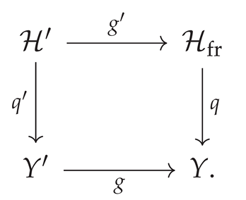
 Assume that the relevant mixed-Hodge-module base-change isomorphism 

$${\beta }_F:g^{*}R{q}_{\sigma }{B}_F\stackrel{\sim }{\to }R{q}_{\sigma }^{\prime }{g}^{\prime *}{B}_F$$

(156)

 holds for $F=I^H,R_{\mathsf{\Sigma }}^H$ and is natural in F. Then 

$${\beta }_{I^H}\left[1\right]\circ g^{*}\left(R{q}_{\sigma }({\rho }^{*}{ϵ}_{\mathsf{\Sigma }}\otimes \mathrm{id})\right)=R{q}_{\sigma }^{\prime }{g}^{\prime *}({\rho }^{*}{ϵ}_{\mathsf{\Sigma }}\otimes \mathrm{id})\circ {\beta }_{R_{\mathsf{\Sigma }}^H}.$$

(157)

 The equality remains valid after applying the same shift and Tate twist to all four corners. 

Proof. 

Apply the naturality of the base-change transformations (156) to ${\rho }^{*}{ϵ}_{\mathsf{\Sigma }}\otimes {\mathrm{id}}_{{\mathcal{K}}_H}$. Its commutative square is (157); the fixed shift and Tate twist commute with every arrow.

□

Proposition 57

(Normalized Gysin benchmark for the forward class).  Let $X=\{\det A=0\}$ be the one-node determinantal conifold and let 

$$X\stackrel{m}{\leftarrow }\tilde{X}\stackrel{q_{\mathrm{line}}}{\to }E,E\simeq {\mathbb{P}}^1,$$

 be the kernel-line resolution and its nonproper vector-bundle projection from Section 5. Let $k:E\hookrightarrow \tilde{X}$ be the zero section. For the nonzero normalized source class ϵ considered in Proposition 31, there is a scalar $\gamma \in {\mathbb{Q}}^{\times }$ such that, relative to the specified local splitting, 

$$m^{*}ϵ=(\gamma g_E,0),g_E:k_{*}{\mathbb{Q}}_E^H(-2)⟶{\mathbb{Q}}_{\tilde{X}}^H\left[4\right].$$

(158)

 Its two direct-image transforms satisfy 

$$R{q}_{\mathrm{line}*}{m}^{*}ϵ=0,R{q}_{\mathrm{line}!}{m}^{*}ϵ=(\gamma \mathrm{id},0)\ne 0.$$

(159)

 If a restriction of the actual Hecke transport diagram is identified with this benchmark by the natural base-change comparison of Lemma 24, the restricted arrow is given by (158) and (159), with the specified normalization and direct-image choice. 

Proof. 

Codimension-two purity identifies the adjoint of $g_E$ with the identity of the Tate orientation line. Propositions 31 and 33 compute both the nonzero Gysin scalar and its vanishing ordinary/nonvanishing exceptional images. Passage to an actual Higgs target additionally requires Lemma 24. □

Remark 29

(Scalar and geometric normalization).  The scalar $\gamma \in {\mathbb{Q}}^{\times }$ is fixed by the chosen source normalization and purity orientation. A one-dimensional Hom group alone does not identify a local Gysin arrow with the target morphism (145); that requires a geometric base-change comparison. 

7.4. Actual Target Adjunction and Fiberwise Gysin Tests

Return to the evaluation-based correspondence of Proposition 50. Fix a bounded coefficient domain, a kernel ${\mathcal{K}}_H$, and the common normalization $[r+d_H]\left(m_H\right)$. Write $\mathcal{H}={\mathcal{H}}_0^{\mathrm{fr}}$, $q=q_{+,0}$ and $J_F=p_{-,0}^{*}{e}_0^{*}F\otimes {\mathcal{K}}_H[r+d_H]\left(m_H\right)$. Let $i_D:D=T\times {\mathbb{P}}^1\hookrightarrow \mathcal{H}$. By projection formula for the closed immersion, $J_{R_X^H}\simeq i_{D*}{V}_D$, for the actual pulled-back kernel coefficient $V_D$ on  D . Denote the pre-target arrow by $\eta :J_{R_X^H}\to J_{I_X^H}\left[1\right]$.

Proposition 58

(Adjunction formula for both target images).  Assume all displayed adjunctions exist in the selected derived MHM category. Under $R{q}_{!}⊣q^{!}$ and $i_{D*}⊣i_D^{!}$, the arrow $R{q}_{!}\left(\eta \right)$ corresponds exactly to the composite 

$$V_D\stackrel{\tilde{\eta }}{\to }{i}_D^{!}{J}_{I_X^H}\left[1\right]\stackrel{i_D^{!}{\mathrm{unit}}_{J_{I_X^H}}\left[1\right]}{\to }{i}_D^{!}{q}^{!}R{q}_{!}{J}_{I_X^H}\left[1\right].$$

(160)

 Under $q^{*}⊣R{q}_{*}$, the arrow $R{q}_{*}\left(\eta \right)$ corresponds to 

$$q^{*}R{q}_{*}{J}_{R_X^H}\stackrel{{\mathrm{counit}}_{J_{R_X^H}}}{\to }{J}_{R_X^H}\stackrel{\eta }{\to }{J}_{I_X^H}\left[1\right].$$

(161)

 The respective target arrows vanish exactly when their displayed adjoints vanish. This reduces the calculation to the actual unit/counit action on the transported Gysin morphism, rather than a choice of generator in a target Hom space. 

Proof. 

Adjunction sends $R{q}_{!}\eta$ to $J_R\stackrel{\eta }{\to }{J}_I\left[1\right]\to q^{!}R{q}_{!}{J}_I\left[1\right]$, the second arrow being the unit. The closed-support adjunction identifies this map with (160). Similarly $q^{*}⊣R{q}_{*}$ sends $R{q}_{*}\eta$ to the composite of the counit $q^{*}R{q}_{*}{J}_R\to J_R$ with $\eta$, proving (161). Since these are Hom-group isomorphisms, they detect zero morphisms faithfully. □

Lemma 25

(Closed-branch detection for the two target images).  Let $i:Z\hookrightarrow H$ be a closed immersion and $q:H\to Y$ a morphism in a six-functor setting. Suppose $\eta :A\to B\left[1\right]$ has $A\simeq i_{*}{i}^{*}A$, and $u:U\hookrightarrow Y$ is open such that $Z_U=Z{\times }_{Y}U\to U$ is an isomorphism. If the restriction of $i^{*}\eta$ to $Z_U$ is nonzero, then both defined maps 

$$u^{*}R{q}_{*}\eta \ne 0,u^{*}R{q}_{!}\eta \ne 0.$$

(162)

 No properness assumption on q is needed. 

Proof. 

Naturality of the adjunction unit $B\to i_{*}{i}^{*}B$ gives a square of arrows $\eta$ and $i_{*}{i}^{*}\eta$. The corresponding map $A\to i_{*}{i}^{*}A$ is an isomorphism by support. Apply either $R{q}_{*}$ or $R{q}_{!}$ and then restrict to  U . Since  i  is proper, $R{q}_{\diamond }{i}_{*}=R{\left(qi\right)}_{\diamond }$, and open restriction commutes with both *- and !-direct image. On  U , the branch map is an isomorphism, so it preserves the nonzero restricted $i^{*}\eta$. If the original target map were zero, its natural comparison to the branch direct image would be zero, a contradiction. □

Theorem 8

(Localized survival on the genuine modified-Higgs target).  Work with the universal determinantal conifold coefficient, the unit Hecke kernel, and the equivariant mixed-Hodge normalization of Lemma 23. Assume the descent comparison specified above, so that the unframed arrow ${\eta }^{\mathrm{un}}$ pulls back to the normalized framed incidence arrow $\eta =p_{-,0}^{*}{e}_0^{*}{ϵ}_X\left[r\right]$. Suppose the stable evaluation-regular source contains a pair $(E_{-},{\theta }_{-})$ with ${\theta }_{-}\left(z\right)=0$ and a line ℓ such that $\gamma \left(J_1{\theta }_{-}\right)(\ell )\ne 0$. Let U be the admissible rank-one target open of Proposition 55, so $D_U\ne ⌀$. Then the genuine unframed unit-kernel target arrows satisfy 

$${\left.R{q}_{+,0*}^{\mathrm{un}}{\eta }^{\mathrm{un}}\right|}_U\ne 0,{\left.R{q}_{+,0!}^{\mathrm{un}}{\eta }^{\mathrm{un}}\right|}_U\ne 0.$$

(163)

 The transported triangles are derived nonsplit on U. This does not imply heart-level ${\mathrm{Ext}}^1$ nonsplitting without perverse concentration, nor transport from unrelated global nodal threefolds or for arbitrary kernels. Common shifts and Tate twists preserve the conclusion. 

Proof. 

The argument has four ingredients. First, smooth evaluation and kernel-branch pullback preserve the nonzero source arrow (Propositions 25 and 49). More precisely, composing its branch restriction with the small-resolution counit gives the nonzero purity-normalized Gysin map of Proposition 31. The codimension-two orientation line remains nonzero after restriction to the nonempty $D_U$; therefore the branch-restricted arrow itself is nonzero. Second, Proposition 55 identifies the unframed kernel branch over  U  with  U . Third, the equivariant coefficient descends with its nonzero costalk normalization by Lemma 23 and the specified smooth-atlas comparison. Finally, the source of the arrow is supported on the closed node locus and hence on the closed kernel branch. Lemma 25 therefore carries the nonzero branch restriction to both actual target images. Lemma 22 proves derived nonsplitting. □

Remark 30

(Why the closed-branch detector has geometric content).  Lemma 25 is formally elementary, but its hypotheses are not automatic: the kernel branch must be recoverable from the target Higgs value, the admissible open must meet the source-node image (Corollary 7), and the selected equivariant Gysin arrow must remain nonzero there. The ordinary image of the same source class vanishes under the distinct nonproper projection $q_{\mathrm{line}}$ of Proposition 33. 

Corollary 7

(Nonempty regular-nilpotent support in the proved genus ranges).  Assume $g\ge 3$ and $h^0(C,{\mathcal{O}}_C\left(2z\right))=1$. For each odd-degree determinant, Theorem 6 and Corollary 3 supply source pairs to which Theorem 8 applies. The same holds in the even-degree cases established in Theorem 7. The exceptional genus-three theta-characteristic case and genus two are excluded from these existence conclusions. 

Proof. 

The existence theorems provide stable $E_{-}$ with surjective first-jet Higgs evaluation and a Higgs field with zero leading value and nonscalar first jet. Its intrinsic quadratic section is nonzero away from its (at most two) zeroes by Proposition 28. For any such line, the modified value is regular nilpotent, so the resulting target lies in  U  by the rank-one inverse and recovery of the chosen stable regular source. Apply the theorem. □

Proposition 59

(Finite degree-two Hecke transport on a saturated open).  Let U be the rank-one determinant-zero target open of Proposition 55. The complete unframed inverse-eigenline incidence $\mathcal{E}\to U$ is finite locally free of degree two. On a trivialization where the $(2,1)$ entry c of the target value is invertible, write 

$$B_{+}\left(0\right)=\left(\begin{array}{cc}a& ad/c\\ c& d\end{array}\right),\mathcal{E}={\mathrm{Spec}}_U{\displaystyle \frac{{\mathcal{O}}_U\left[v\right]}{\left(\right(v-a\left)\right(v+d\left)\right)}}.$$

(164)

 Let ${\mathcal{E}}^{\circ }$ be the open on which the corresponding upper inverse modifications have stable, evaluation-regular source. Then 

$$U^{\prime }:=U\setminus \mathrm{im}(\mathcal{E}\setminus {\mathcal{E}}^{\circ })$$

(165)

 is an open substack containing the admissible regular-nilpotent source-node images of Corollary 7. The complete unframed Hecke correspondence over $U^{\prime }$ is the finite locally free degree-two cover $q^{\prime }{:\mathcal{E}|}_{U^{\prime }}\to U^{\prime }$. In the selected bounded MHM category, the canonical comparison $R{q}_{!}^{\prime }\stackrel{\sim }{\to }R{q}_{*}^{\prime }$ is an isomorphism. The same assertion is not made for the original framed map ${\mathcal{H}}_0^{\mathrm{fr}}\to U^{\prime }$ or for $q_{\mathrm{line}}$. 

Proof. 

An inverse upper modification is regular exactly when its target line is invariant under $B_{+}\left(0\right)$. No invariant line equals $\mathbb{C}(1,0)$ in the displayed chart because  c  is invertible. Writing the line as $\mathbb{C}(u,1)$, its equation is $c{u}^2+(d-a)u-ad/c=0$. Setting $v=cu$ gives the monic polynomial $(v-a)(v+d)$, so $\mathcal{E}$ is free over ${\mathcal{O}}_U$ with basis $1,v$. The construction is intrinsic and glues under change of target frame. Its two geometric lines are the image and kernel for nonzero trace; at trace zero they meet in a length-two scheme supported on their common line. Stability and the condition $H^0(C,{\mathrm{End}}_0{E}_{-}\left(z\right))=0$ are open in reconstructed families. Hence $\mathcal{E}\setminus {\mathcal{E}}^{\circ }$ is closed, and its image is closed because $\mathcal{E}\to U$ is finite. Over $U^{\prime }$ every inverse line is admissible, identifying the restricted Hecke correspondence with the full finite incidence. At an admissible regular-nilpotent source-node image there is exactly one geometric invariant line, which is the original marked line. Its inverse recovers the stable evaluation-regular source, so the closed inadmissible locus has empty fiber there; these points belong to $U^{\prime }$. Finally a finite morphism is proper, hence the two derived direct images coincide on their common domain. □

Theorem 9

(Nonzero degree-two derived attachment on the finite target open).  Assume the unit kernel, the specified equivariant mixed-Hodge lift of Lemma 23, and a compatible unframed quotient-stack MHM formalism with the normalized smooth-atlas exchange of Proposition 68 and Lemma 27. Let $U^{\prime }\subset U$ be the nonempty saturated open of Proposition 59. Denote by $J_I^{\mathrm{un}}$ and ${\widehat{R}}^{\mathrm{un}}$ the descent-normalized perverse objects on the unframed correspondence, with fixed relative atlas dimension $g_F$ and $F_{\mathcal{H}}^{*}\left[g_F\right]J_I^{\mathrm{un}}\simeq J_I$, $F_{\mathcal{H}}^{*}\left[g_F\right]{\widehat{R}}^{\mathrm{un}}\simeq \widehat{R}$. Their framed models are 

$$J_I=p_{-,0}^{*}{e}_0^{*}{I}_X^H\left[r\right],J_R=p_{-,0}^{*}{e}_0^{*}{R}_X^H\left[r\right]=\widehat{R}[-1].$$

(166)

 Existence and these perverse degrees on the framed incidence space are those of Corollary 4; the stated descent comparison is required to transport them to the unframed category. Define the target perverse objects 

$$I^{\prime }:=q_{*}^{\prime }{J}_I^{\mathrm{un}},R^{\prime }:=q_{*}^{\prime }{\widehat{R}}^{\mathrm{un}}\in \mathrm{MHM}\left(U^{\prime }\right).$$

(167)

 Then the genuinely transported forward arrow is a nonzero class 

$$0\ne \left[{ϵ}_{U^{\prime }}\right]\in {\mathrm{Hom}}_{{\mathsf{D}}_H\left(U^{\prime }\right)}(R^{\prime },I^{\prime }\left[2\right]).$$

(168)

 Its middle coefficient $P^{\prime }$ has precisely ${}^p{\mathcal{H}}^0\left(P^{\prime }\right)\simeq I^{\prime }$ and ${}^p{\mathcal{H}}^1\left(P^{\prime }\right)\simeq R^{\prime }$, with the nonzero class as its derived Postnikov attachment. It is not a heart-level ${\mathrm{Ext}}^1$ class between $R^{\prime }$ and $I^{\prime }$. The theorem is not an assertion about an unrestricted framed pushforward, general correspondence kernels, or unrelated multi-node degenerations. 

Proof. 

Proposition 30 proves that $p_0^{*}{I}_X^H$ is perverse on the  complete  normal-crossing incidence fiber. Smooth evaluation with shift $\left[r\right]$ therefore gives a perverse $J_I$. The node inverse image is a smooth subvariety of dimension $r+1$, so the quotient $J_R$ lies in perverse degree one and equals $\widehat{R}[-1]$. The assumed equivariant smooth-atlas comparison, normalized by its relative dimension, carries these two degree statements to $J_I^{\mathrm{un}}$ and ${\widehat{R}}^{\mathrm{un}}$. The map $q^{\prime }$ is finite, hence its direct image is perverse  t -exact and $R{q}_{!}^{\prime }\simeq R{q}_{*}^{\prime }$; therefore $I^{\prime }$ and $R^{\prime }$ lie in the target heart. The descended connecting arrow has source $R^{\prime }[-1]$ and target $I^{\prime }\left[1\right]$, hence has degree two as in (168). It is nonzero: $U^{\prime }$ contains a source-node image, and the purity/Gysin branch restriction used in the proof of Theorem 8 remains nonzero on this smaller open. The closed-branch detector applies there as well. The long exact perverse cohomology sequence of the transported triangle gives the two stated perverse cohomology objects of $P^{\prime }$; its attachment is the same connecting morphism under the displayed shift identification. □

Remark 31

(Why the finite-open statement is genuinely stronger).  Theorem 8 detects a nonzero derived arrow on U without properness. On $U^{\prime }$ the full unframed inverse correspondence becomes finite, the ordinary and exceptional images agree, and the chosen extension acquires the precise degree-two placement (168). This does not imply perverse concentration of the transported middle object, which instead has nontrivial Postnikov data; nor does it identify the finite map with the nonproper affine-jet projections of Section 6.4. Once $q^{\prime }$ is finite, the degree-two placement of $\left[{ϵ}_{U^{\prime }}\right]$ follows formally from the perverse degrees $J_I\in \mathrm{MHM}$ and $J_R\simeq \widehat{R}[-1]$; the geometric content lies in establishing that formal argument’s hypotheses, namely the perversity of $p_0^{*}{\mathrm{IC}}_X^H$ on the reducible incidence fiber (Proposition 5.2), the finiteness of the full inverse correspondence over $U^{\prime }$ together with the fact that $U^{\prime }$ contains the source-node image (Proposition 7.23), and the survival of the class there (Theorem 7.20). 

Proposition 60

(Pointwise restrictions of the target morphism).  For a geometric target point y and its Cartesian fiber $F_y=q^{-1}\left(y\right)$ with inclusion $j_y:F_y\hookrightarrow \mathcal{H}$, pointwise compact-support base change, whenever valid in the chosen MHM setting, gives 

$$i_y^{*}R{q}_{!}\left(\eta \right)\simeq R{\mathsf{\Gamma }}_c(F_y,j_y^{*}\eta ).$$

(169)

 For the ordinary image, the analogous stalk formula requires the appropriate *-exchange (for example, properness on the coefficient support). In a proper setting with extraordinary exchange, one also has 

$$i_y^{!}R{q}_{*}\left(\eta \right)\simeq R\mathsf{\Gamma }(F_y,j_y^{!}\eta ).$$

(170)

 These are natural identifications of morphisms ; their targets cannot be calculated from fiber cohomology alone without determining the actual extraordinary Gysin/excess-intersection maps. 

Proof. 

Apply the indicated base-change transformations to the morphism $\eta$, not just its endpoints. The first uses compact-support pointwise exchange, and the second is the extraordinary exchange under the stated properness hypotheses. Naturality transports the source arrow to the displayed maps of fiber cohomology. □

Remark 32

(Why scalar-target stalks do not detect the forward class).  Suppose $y=(F,{\theta }_{+})$ has ${\theta }_{+}\left(z\right)=0$ and scalar first target jet. If the inverse fiber is the complete $\mathbb{P}\left(F_z\right)$, the source evaluation factors through o, and the fiberwise arrow is the pullback of ${ϵ}_X$, then 

$$i_y^{*}{ϵ}_{+,!}=0.$$

(171)

 If the ordinary-image base-change comparison is also an isomorphism, then $i_y^{*}{ϵ}_{+,*}=0$. The vanishing is already forced by $i_o^{*}{ϵ}_X=0$ (Lemma 2), so it is not an independent extension-survival test. The extraordinary target restriction remains the relevant local diagnostic. 

Proof. 

Proposition 54 gives the complete inverse source-node fiber under the scalar-target-jet assumption. The other hypotheses identify the coefficient morphism on that fiber with the pullback of $i_o^{*}{ϵ}_X$. But $i_o^{*}{I}_X^H\left[1\right]\simeq {\mathbb{Q}}^H\left[4\right]\oplus {\mathbb{Q}}^H(-1)\left[2\right]$ and the rational MHS category has cohomological dimension one, so $\mathrm{Hom}({\mathbb{Q}}^H(-2),i_o^{*}{I}_X^H\left[1\right])=0$. Hence the fiberwise arrow is zero; apply (169), and, when its hypotheses hold, the ordinary *-exchange. □

Remark 33

(Remaining extraordinary Gysin computation).  The first source jet determines the target Higgs value , but the target first jet depends on the second source jet; see Corollary 6. Furthermore the normal sequences (149)– (150) concern fixed-source curves, not the full differential of q along $T\times {\mathbb{P}}^1$. Theorem 8 now detects the unit-kernel target arrow over the admissible rank-one open by a branch inverse, not by this scalar-stalk test. The extraordinary fiber map $j_y^{!}\eta$ and the unit composite (160) remain to be calculated on other strata and for general kernels or unrelated global sources. 

7.5. Local Stalk/Costalk Extension Tests

Fix a closed immersion $i:Z\hookrightarrow Y$ and its open complement $j:U\hookrightarrow Y$. For $†\in \{*,!\}$ write

$$I_Z^{†}:=i^{†}{I}_Y,P_Z^{†}:=i^{†}{P}_Y,R_Z^{†}:=i^{†}{R}_Y,$$

where $i^{*}=i^{*}$ and $i^{!}=i^{!}$; cohomology on  Z  refers to the standard  t -structure of $D^b\mathrm{MHM}\left(Z\right)$.

Proposition 61

(Exact stalk and costalk sequences).  For every integer n and either choice †, restriction of (139) gives the exact sequence 

$$\begin{array}{cc}\hfill \dots ⟶{\mathcal{H}}^n\left(I_Z^{†}\right)& \stackrel{a_{Z,n}^{†}}{\to }{\mathcal{H}}^n\left(P_Z^{†}\right)\stackrel{b_{Z,n}^{†}}{\to }{\mathcal{H}}^n\left(R_Z^{†}\right)\hfill \\ \hfill & \stackrel{{\delta }_{Z,n}^{†}}{\to }{\mathcal{H}}^{n+1}\left(I_Z^{†}\right)⟶\dots ,\hfill \end{array}$$

(172)

 with 

$${\delta }_{Z,n}^{†}={\mathcal{H}}^n\left(i^{†}{ϵ}_Y\right).$$

(173)

 For every geometric point $z\in Z$, if the restricted rational stalk or costalk cohomology groups are finite-dimensional, then 

$$\begin{array}{cc}\hfill {\mathrm{rank}}_{\mathbb{Q}}{\delta }_{z,n}^{†}& ={\dim }_{\mathbb{Q}}\mathrm{coker}{b}_{z,n}^{†}\hfill \\ \hfill & ={\dim }_{\mathbb{Q}}\ker a_{z,n+1}^{†}.\hfill \end{array}$$

(174)

 These equalities determine the ranks once the actual geometric maps $a_Y,b_Y$ are calculated; ranks of the endpoint objects alone do not determine the boundary maps. 

Proof. 

The exact derived functors $i^{*}$ and $i^{!}$ preserve the transported triangle. Its long exact cohomology sequence gives (172) and ${\delta }_{Z,n}^{†}={\mathcal{H}}^n\left(i^{†}{ϵ}_Y\right)$. At a point, $\mathrm{im}{b}_{z,n}^{†}=\ker {\delta }_{z,n}^{†}$ and $\mathrm{im}{\delta }_{z,n}^{†}=\ker a_{z,n+1}^{†}$; rank–nullity yields (174).

□

Proposition 62

(Calculated local boundary ranks).  Retain the one-node correspondence of Proposition 57. For any $y\in E$, let $i_y:\left\{y\right\}\hookrightarrow E$, and let ${\delta }_{\sigma ,n}^{†}$ be the connecting map obtained from the transported triangle under $R{q}_{\mathrm{line}\sigma }{m}^{*}$ and then $i_y^{†}$, with $\sigma \in \{*,!\}$. After rational realization, the connecting maps satisfy 

$$\mathrm{rank}{\delta }_{!,0}^{*}=1,\mathrm{rank}{\delta }_{*,n}^{*}=0\mathrm{for}\mathrm{every}n,$$

(175)

 and 

$$\mathrm{rank}{\delta }_{!,2}^{!}=1,\mathrm{rank}{\delta }_{*,n}^{!}=0\mathrm{for}\mathrm{every}n.$$

(176)

 All other connecting maps for the compactly supported benchmark vanish. The nonzero maps have Tate type ${\mathbb{Q}}^H(-2)\to {\mathbb{Q}}^H(-2)$ on stalks and ${\mathbb{Q}}^H(-3)\to {\mathbb{Q}}^H(-3)$ on costalks. 

Proof. 

The ordinary connecting arrow vanishes by (159). The exceptional arrow is $\gamma \mathrm{id}$ on ${\mathbb{Q}}_E^H(-2)$ and zero on the other summand. Its stalk at  y  is nonzero in degree zero. Purity for $i_y:\left\{y\right\}\hookrightarrow E$ gives $i_y^{!}{\mathbb{Q}}_E^H(-2)\simeq {\mathbb{Q}}_{\left\{y\right\}}^H(-3)[-2]$; thus its costalk map has rank one in degree two. All remaining components vanish.

□

Lemma 26

(Attaching-map compatibility).  Assume the chosen two-stratum geometry $(U,Z)$ admits the MacPherson–Vilonen presentation fixed in Definition 25. Let $M,M^{\prime }\in \mathrm{MHM}\left(Y\right)$ correspond to data $(A,B,u,v)$ and $(A^{\prime },B^{\prime },u^{\prime },v^{\prime })$, with a transported morphism $h:M\to M^{\prime }$ and restrictions $\alpha :A\to A^{\prime }$ and $\beta :B\to B^{\prime }$. Then 

$$\beta u=u^{\prime }F\left(\alpha \right),G\left(\alpha \right)v=v^{\prime }\beta .$$

(177)

 In particular the corresponding closed-stratum connecting maps and their kernels and cokernels must agree with the stalk/costalk boundaries of Proposition 61. Without the specified gluing equivalence, equations (177) are necessary compatibility relations, not a uniqueness theorem for h in the derived category. 

Proof. 

Naturality of the adjunction maps $j_{!}{j}^{*}M\to M\to R{j}_{*}{j}^{*}M$ gives a morphism of recollement triangles. Their perverse kernels and cokernels yield $\beta u=u^{\prime }F\left(\alpha \right)$ and $G\left(\alpha \right)v=v^{\prime }\beta$. These equations constrain the gluing maps; a derived uniqueness claim needs the specified MV equivalence.

□

7.6. Nonvanishing, Splitting, or Obstruction

For the universal local coefficient, the target arrow is defined by (145); for a separately verified global realization it is (142). Its splitting is detected by extraordinary restriction to the support of the transported quotient.

Proposition 63

(Closed-support detection of the transported class).  Let $\mathsf{H}$ satisfy Definition 28. Suppose there is a closed immersion $i:Z\hookrightarrow Y$, an object $V\in {\mathsf{D}}_H\left(Z\right)$, and a specified isomorphism 

$$\alpha :i_{*}V\stackrel{\sim }{\to }{R}_Y.$$

(178)

 Let 

$${\widetilde{ϵ}}_Y:V\stackrel{\sim }{\to }{i}^{!}{i}_{*}V\stackrel{i^{!}\left({ϵ}_Y\alpha \right)}{\to }{i}^{!}{I}_Y\left[1\right]$$

(179)

 be the adjoint of ${ϵ}_Y\alpha$. Then: 

(i)

 ${ϵ}_Y=0$ if and only if ${\widetilde{ϵ}}_Y=0$ in ${\mathsf{D}}_H\left(Z\right)$. 

(ii)

 The transported distinguished triangle splits if and only if ${\widetilde{ϵ}}_Y=0$. 

(iii)

 If both $I_Y$ and $R_Y$ belong to $\mathrm{MHM}\left(Y\right)$, the nonzero class ${\widetilde{ϵ}}_Y$ determines a nonsplit short exact sequence (140). Without this perverse concentration, nonvanishing is a statement about the derived connecting morphism, not automatically about a target-heart Yoneda ${\mathrm{Ext}}^1$ class. 

Proof. 

Closed-embedding adjunction provides

$${\mathrm{Hom}}_{{\mathsf{D}}_H\left(Y\right)}(i_{*}V,I_Y\left[1\right])\simeq {\mathrm{Hom}}_{{\mathsf{D}}_H\left(Z\right)}(V,i^{!}{I}_Y\left[1\right]).$$

(180)

It carries ${ϵ}_Y\alpha$ to ${\widetilde{ϵ}}_Y$. This proves (i). The distinguished-triangle splitting criterion proves (ii), and extension closure of the MHM heart proves (iii).

□

Corollary 8

(A geometric nonvanishing test).  In the hypotheses of Proposition 63, assume there exists a map $h:Z^{\prime }\to Z$ for which $h^{!}{\widetilde{ϵ}}_Y$ is defined and is nonzero. Then ${ϵ}_Y\ne 0$. In particular, a verified Cartesian restriction identifying $h^{!}{\widetilde{ϵ}}_Y$ with a nonzero, purity-normalized Gysin map proves derived nonsplitting on Y. 

Proof. 

A functor takes the zero morphism to zero. Therefore $h^{!}{\widetilde{ϵ}}_Y\ne 0$ implies ${\widetilde{ϵ}}_Y\ne 0$. Proposition 63(i)–(ii) gives the conclusion. The qualification “verified” is essential: equality of target Hom dimensions does not identify the actual restricted map with the Gysin generator. □

Proposition 64

(Postnikov placement when perverse concentration fails).  Let $\mathsf{H}$ be as above and suppose $R_Y\simeq T[-r]$ with $T\in \mathrm{MHM}\left(Y\right)$ and $r\in \mathbb{Z}$. Then 

$${ϵ}_Y\in {\mathrm{Hom}}_{{\mathsf{D}}_H\left(Y\right)}(T,I_Y[r+1]).$$

(181)

 If, in addition, $I_Y\simeq J[-s]$ for $J\in \mathrm{MHM}\left(Y\right)$, the transported arrow belongs to 

$${\mathrm{Hom}}_{{\mathsf{D}}_H\left(Y\right)}(T,J[r-s+1]).$$

(182)

 For a finite-type variety Y with ${\mathsf{D}}_H\left(Y\right)=D^b\mathrm{MHM}\left(Y\right)$, this is the Yoneda group ${\mathrm{Ext}}_{\mathrm{MHM}\left(Y\right)}^{r-s+1}(T,J)$ when $r-s+1\ge 0$; no such identification is presumed on a stack. In general, when $I_Y$ has several nonzero perverse degrees, ${ϵ}_Y$ must be retained as a derived morphism, and its interaction with the Postnikov truncation triangles must be calculated before identifying a single Yoneda class. 

Proof. 

The shift isomorphisms give $\mathrm{Hom}(R_Y,I_Y\left[1\right])\simeq \mathrm{Hom}(T,I_Y[r+1])$. If $I_Y\simeq J[-s]$, this is $\mathrm{Hom}(T,J[r-s+1\left]\right)$, giving (182). Without concentration of $I_Y$, its Postnikov attachments prevent a canonical reduction to a single heart-level Ext group.

□

Remark 34

(Verified outcome and remaining target computation).  Smooth evaluation and incidence pullback preserve the local class (Proposition 49). The differential and noncontraction calculations of Propositions 51– 53 and the inverse-jet stratification of Proposition 54 now constrain the actual target geometry. The target morphism is defined by (145), with its adjoints computed in Proposition 58. The rank-one branch inverse and localized Gysin detection prove unit-kernel target nonvanishing on U (Theorem 8); on $U^{\prime }$, Theorem 9 identifies its nonzero degree-two derived class. The remaining extraordinary fiber Gysin and Postnikov computations concern other target strata, kernels, and global source realizations. The ${\mathbb{P}}^1$ benchmark in (159) cannot replace that map; framing descent is treated in Section 8. 

7.7. Compatibility with the Node-Supported Interface

In addition to (137), the corrected source package contains the distinct node-interface diagram

$${\mathsf{\Psi }}^H\stackrel{u_{\mathsf{\Sigma }}}{\to }{Q}_{\mathsf{\Sigma }}^H\stackrel{v_{\mathsf{\Sigma }}}{\to }{\mathsf{\Psi }}^H(-1),N_{\mathsf{\Sigma }}^H=v_{\mathsf{\Sigma }}{u}_{\mathsf{\Sigma }},$$

(183)

where $Q_{\mathsf{\Sigma }}^H={⨁}_k{i}_{k*}{\mathbb{Q}}_{\left\{p_k\right\}}^H(-1)$, in contrast to $R_{\mathsf{\Sigma }}^H={⨁}_k{i}_{k*}{\mathbb{Q}}_{\left\{p_k\right\}}^H(-2)$.

Proposition 65

(Transport of the two distinct diagrams).  Assume $\mathsf{H}$ is defined on every object and arrow of both (137) and (183). Then it carries the interface to 

$$\mathsf{H}\left({\mathsf{\Psi }}^H\right)\stackrel{\mathsf{H}\left(u_{\mathsf{\Sigma }}\right)}{\to }\mathsf{H}\left(Q_{\mathsf{\Sigma }}^H\right)\stackrel{\mathsf{H}\left(v_{\mathsf{\Sigma }}\right)}{\to }\mathsf{H}\left({\mathsf{\Psi }}^H\right)(-1),$$

(184)

 with 

$$\mathsf{H}\left(N_{\mathsf{\Sigma }}^H\right)=\mathsf{H}\left(v_{\mathsf{\Sigma }}\right)\circ \mathsf{H}\left(u_{\mathsf{\Sigma }}\right).$$

(185)

 The forward connecting arrow (142) is separately transported. No isomorphism between $\mathsf{H}\left(Q_{\mathsf{\Sigma }}^H\right)$ and $\mathsf{H}\left(R_{\mathsf{\Sigma }}^H\right)$, and no identification between $\mathsf{H}\left({ϵ}_{\mathsf{\Sigma }}\right)$ and a canonical or variation map, follows from the proposition. 

Proof. 

The functor $\mathsf{H}$ respects composition and Tate twist. Applying it to the two arrows in (183) yields (184) and (185). The forward Yoneda arrow has the distinct coefficient $R_{\mathsf{\Sigma }}^H$ and remains separately typed.

□

Theorem 10

(Conditional family-level specialization compatibility).  Suppose the verified correspondence datum extends over a common one-parameter base and gives a proper morphism of degeneration families $g:\mathcal{Y}\to \mathcal{X}$ over that base, with induced special-fiber map $g_0:Y_0\to X_0$. Assume the source MHM coefficients and their correspondence kernels admit the indicated family-level lifts and that all specialization base-change morphisms in use are isomorphisms. Then the natural comparisons 

$${\kappa }_{\mathsf{\Psi }}:{\psi }_{\pi ,1}^H\left(R{g}_{*}M\right)\stackrel{\sim }{\to }R{g}_{0*}{\psi }_{f,1}^H\left(M\right),{\kappa }_{\mathsf{\Phi }}:{\varphi }_{\pi ,1}^H\left(R{g}_{*}M\right)\stackrel{\sim }{\to }R{g}_{0*}{\varphi }_{f,1}^H\left(M\right),$$

 for any such $M\in {\mathsf{D}}_H\left(\mathcal{Y}\right)$, intertwine ${\mathrm{can}}^H$, ${\mathrm{Var}}^H$, and nilpotent monodromy, with their Tate twists. For any morphism of eligible family-level coefficients, these comparisons commute with that morphism. Consequently, if a family-level morphism lifts ${ϵ}_{\mathsf{\Sigma }}$, its Hecke image is compatible with specialization through the resulting naturality diagrams. 

Proof. 

Proper direct image commutes with the stated normalized nearby and vanishing cycles. Naturality of ${\mathrm{can}}^H$ and ${\mathrm{Var}}^H$ yields their commutative squares, including the $(-1)$ twist; their composite gives the monodromy square. The same natural transformations are compatible with a family-level morphism representing ${ϵ}_{\mathsf{\Sigma }}$ when such a lift is specified [3,25].

□

Remark 35

(Local support versus global limiting mixed Hodge structure).  The forward quotient $R_{\mathsf{\Sigma }}^H$ has Tate type $(-2)$, whereas $Q_{\mathsf{\Sigma }}^H$ has type $(-1)$; neither their morphisms nor their images are identified by support alone. The rank $c\le r$ of globally independent vanishing cycles (Remark 1) is distinct from the nodewise local direct sum. Specialization and bounded composition are considered in Section 9. 

8. Framing-Forgetting and Extension Defects

We compare the corrected forward extension on framed and unframed Hecke–Higgs targets. Theorem 8 proves unit-kernel derived nonvanishing on the admissible rank-one target open  U ; Theorem 9 sharpens its perverse placement over the saturated open $U^{\prime }\subset U$. Here we verify the compatible atlas comparisons without treating the nonproper framing torsor as a finite correspondence. Fiber frames, higher-jet groupoids, and the intrinsic unframed Hecke correspondence play distinct roles. We retain the local Euler-class and atlas-unit residual as separate auxiliary constructions, not as substitutes for the forward Gysin morphism.

8.1. The Actual Framing-Forgetting Morphism

Fix the lower modification of Definition 6. For $N\ge 2$, write $R_N=\mathbb{C}\left[w\right]/\left(w^{N+1}\right)$ and $G_N=G{L}_2\left(R_N\right)$. Thus $G_N$ is smooth affine of dimension $g_N=4(N+1)$. It acts on source or target Higgs jets by formal change of frame; in an invariant-line chart, a change of adapted source frame induces the modified transition $g_{+}=D^{-1}gD$ of (48). The latter is regular only for a transition preserving the relevant Hecke lattice.

Definition 29

(Framing quotient on a finite-type chart).  Let $W_{+}^{\mathrm{fr}}$ be a finite-type $G_N$-scheme parametrizing modified Higgs N-jets, and suppose its unframed finite-jet moduli stack is ${\mathcal{Y}}_{+}=[W_{+}^{\mathrm{fr}}/G_N]$. The forgetful atlas is 

$$F_{+}:W_{+}^{\mathrm{fr}}⟶{\mathcal{Y}}_{+}.$$

(186)

 The full Higgs-moduli target of Proposition 26 requires descent of actual bundle and Higgs-field families; the quotient of truncated jet coordinates is not that global target. In particular, the fixed-line value chart $Y_{+}^{\mathrm{ad},0}$ of (112) is not a $G_N$-stable atlas. We also distinguish the rank-two frame torsor at z, with structure group $G_0=G{L}_2\left(\mathbb{C}\right)$, from the full jet-framing groupoid: a framing of ${E|}_z$ alone does not fix the modified first Higgs jet. 

Proposition 66

(Geometry of the quotient atlas).  The map $F_{+}$ is representable, smooth, and surjective of relative dimension $g_N$. Its base change by any geometric point of ${\mathcal{Y}}_{+}$ is a $G_N$-torsor, noncanonically isomorphic to $G_N$. It is not proper. The automorphism group of the image of a framed point x is its stabilizer ${\left(G_N\right)}_x$. 

Proof. 

An object of $[W_{+}^{\mathrm{fr}}/G_N]$ over  T  is a principal $G_N$-bundle $P\to T$ with an equivariant map $P\to W_{+}^{\mathrm{fr}}$. Its pullback of (186) is $P\to T$. Since $G_N$ is smooth of dimension $4(N+1)$, this proves representability, smoothness, and surjectivity. A geometric torsor is trivial after a choice of point; its fiber is the nonproper positive-dimensional affine group $G_N$, so $F_{+}$ is not proper. Automorphisms of an object with chosen representative  x  are exactly the elements fixing  x . □

Remark 36

(Stabilizers and coarse quotients).  The stabilizers of Proposition 11 are already nontrivial at jet order zero and increase on the scalar locus. Thus $[W_{+}^{\mathrm{fr}}/G_N]$ is not replaced by an orbit space. The atlas $F_{+}$ is also distinct from $q_{\mathrm{line}}:\tilde{X}\to {\mathbb{P}}^1$ in Section 5. 

Definition 30

(Descent of a Hecke correspondence).  Let $W_{-}^{\mathrm{fr}}\stackrel{p_{\mathrm{fr}}}{\leftarrow }{\mathcal{H}}_{\mathrm{fr}}\stackrel{q_{\mathrm{fr}}}{\to }{W}_{+}^{\mathrm{fr}}$ be a finite-type framed Hecke correspondence. A descent datum consists of compatible source, incidence, and modified-target frame groupoids, a span ${\mathcal{Y}}_{-}\stackrel{p_{\mathrm{un}}}{\leftarrow }{\mathcal{H}}_{\mathrm{un}}\stackrel{q_{\mathrm{un}}}{\to }{\mathcal{Y}}_{+}$, and atlases $F_{-},F_{\mathcal{H}},F_{+}$ giving 2-Cartesian squares for both projections. It includes an equivariant kernel ${\mathcal{K}}_{\mathrm{fr}}$ descended from ${\mathcal{K}}_{\mathrm{un}}$, with 

$$F_{\mathcal{H}}^{*}{\mathcal{K}}_{\mathrm{un}}\stackrel{\sim }{\to }{\mathcal{K}}_{\mathrm{fr}},$$

(187)

 and a specified bounded mixed-Hodge-module formalism on the chosen quotient stacks. A different source and target jet order, as required by (42), is accommodated by the corresponding two action groupoids rather than an assumed map $G_N\to G_N$. 

Remark 37

(Local status of the descent datum).  The frame-change identity (49) defines the morphism of higher-jet change-of-frame groupoids, while the elementary modification of Proposition 26 is intrinsically defined on families of bundles. The rank-one inverse of Proposition 55 is an isomorphism of the resulting unframed Hecke groupoids, not a map inverse to a framed-source scheme over an unframed target. The finite-jet quotient (186) becomes a suitable atlas only with the stated 2-Cartesian comparison to the actual Higgs stack and kernel descent. In particular, the finite degree-two map $q^{\prime }$ of Proposition 59 is unframed ; pulling it back along an appropriate target atlas produces another finite map, but does not make the original framed-to-unframed map finite. 

Proposition 67

(Evaluation incidence on the fiber-frame quotient).  Let $G=G{L}_2\left(\mathbb{C}\right)$, and let $B^{\circ ,\mathrm{fr}}$ be a G-stable fiber-frame atlas for the evaluation-regular source locus. Let $e:{\mathcal{Y}}_{-}^{\mathrm{fr}}\to M$ and $p:\mathcal{I}\to M$ be the G-equivariant evaluation and incidence maps. On the corresponding quotient stacks there is a canonical 2-Cartesian presentation 

$$[{\mathcal{Y}}_{-}^{\mathrm{fr}}{\times }_M\mathcal{I}/G]\simeq [{\mathcal{Y}}_{-}^{\mathrm{fr}}/G]{\times }_{[M/G]}[\mathcal{I}/G].$$

(188)

 The same holds over the determinant-zero locus and for its kernel-line branch. The source class ${ϵ}_X$ admits the selected equivariant lift of Lemma 23; its normalized pullback along evaluation and incidence is compatible with the quotient atlas and with the original nonzero costalk scalar. Equation (188) does not identify the higher-jet quotient in Definition 29 with the global modified-Higgs stack. 

Proof. 

An object on the right over a test scheme consists of a  G -torsor, an equivariant source Higgs family, and an equivariant invariant line with matching evaluated leading matrix. This is precisely a  G -torsor with an equivariant map to ${\mathcal{Y}}_{-}^{\mathrm{fr}}{\times }_M\mathcal{I}$, the moduli problem on the left. These descriptions preserve morphisms and arbitrary base change. The equations $\det A=0$ and $A\ell =0$ are  G -invariant, so taking either closed locus commutes with the construction. The equivariant class is the costalk lift of Lemma 23. Its pullback to any nonempty smooth evaluation atlas is the same nonzero Tate-normalized scalar by Proposition 25; no general faithfulness assertion for arbitrary derived Hom groups is used. □

Remark 38

(Two distinct framing groupoids).  The quotient in (188) uses fiber frames at z and suffices for the leading invariant-line incidence. The modified first jet requires source second-jet data and the full adapted-frame transitions of Proposition 10. The genuine inverse in Proposition 55 is defined using the intrinsic image line of the target Higgs value; it does not depend on choosing either sort of frame. 

8.2. Derived Comparison Under Forgetting Framing

Let ${\mathsf{S}}_{\mathrm{un}}$ be a source realization on ${\mathcal{Y}}_{-}$, with framed counterpart ${\mathsf{S}}_{\mathrm{fr}}$. Assume a natural comparison on the corrected source triangle,

$$F_{-}^{*}{\mathsf{S}}_{\mathrm{un}}\left(M\right)\stackrel{\sim }{\to }{\mathsf{S}}_{\mathrm{fr}}\left(M\right),M\in \{I^H,P^H,R_{\mathsf{\Sigma }}^H\},$$

(189)

compatible with its three arrows. For the universal local conifold on the evaluation-regular locus, the framed realization is the smooth evaluation pullback of Proposition 24.

Proposition 68

(Base-change comparison of Hecke transforms).  Assume Definition 30, (189), and the requisite mixed-Hodge-module exchange isomorphisms for the 2-Cartesian square 

$$\begin{array}{ccc}{\mathcal{H}}_{\mathrm{fr}}& \stackrel{F_{\mathcal{H}}}{\to }& {\mathcal{H}}_{\mathrm{un}}\\ q_{\mathrm{fr}}\downarrow & & \downarrow q_{\mathrm{un}}\\ W_{+}^{\mathrm{fr}}& \stackrel{F_{+}}{\to }& {\mathcal{Y}}_{+}.\end{array}$$

(190)

 For $\sigma \in \{*,!\}$, fix $d,m\in \mathbb{Z}$ and define the unframed transform ${\mathsf{H}}_{\mathrm{un}}\left(M\right)=R{q}_{\mathrm{un},\sigma }(p_{\mathrm{un}}^{*}{\mathsf{S}}_{\mathrm{un}}\left(M\right)\otimes {\mathcal{K}}_{\mathrm{un}})\left[d\right]\left(m\right)$ and similarly ${\mathsf{H}}_{\mathrm{fr}}$ using the framed span and kernel. On the specified bounded coefficient category there is a natural isomorphism 

$${\beta }_M:F_{+}^{*}{\mathsf{H}}_{\mathrm{un}}\left(M\right)\stackrel{\sim }{\to }{\mathsf{H}}_{\mathrm{fr}}\left(M\right).$$

(191)

 Writing ${ϵ}_{\mathrm{un}}={\mathsf{H}}_{\mathrm{un}}\left({ϵ}_{\mathsf{\Sigma }}\right)$ and ${ϵ}_{\mathrm{fr}}={\mathsf{H}}_{\mathrm{fr}}\left({ϵ}_{\mathsf{\Sigma }}\right)$, its naturality gives the commutative square 

$$\begin{array}{ccc}{F}_{+}^{*}{\mathsf{H}}_{\mathrm{un}}\left(R_{\mathsf{\Sigma }}^H\right)& \stackrel{F_{+}^{*}{ϵ}_{\mathrm{un}}}{\to }& F_{+}^{*}{\mathsf{H}}_{\mathrm{un}}\left(I^H\right)\left[1\right]\\ {\beta }_{R_{\mathsf{\Sigma }}^H}\downarrow & & \downarrow {\beta }_{I^H}\left[1\right]\\ {\mathsf{H}}_{\mathrm{fr}}\left(R_{\mathsf{\Sigma }}^H\right)& \stackrel{{ϵ}_{\mathrm{fr}}}{\to }& {\mathsf{H}}_{\mathrm{fr}}\left(I^H\right)\left[1\right].\end{array}$$

(192)

Proof. 

Put $K_M=p_{\mathrm{un}}^{*}{\mathsf{S}}_{\mathrm{un}}\left(M\right)\otimes {\mathcal{K}}_{\mathrm{un}}$. The exchange for (190) is

$$F_{+}^{*}R{q}_{\mathrm{un},\sigma }{K}_M⟶R{q}_{\mathrm{fr},\sigma }{F}_{\mathcal{H}}^{*}{K}_M.$$

By the source square, (189), and (187), the coefficient on the right is $p_{\mathrm{fr}}^{*}{\mathsf{S}}_{\mathrm{fr}}\left(M\right)\otimes {\mathcal{K}}_{\mathrm{fr}}$. The assumed exchange isomorphism gives (191) after $\left[d\right]\left(m\right)$. Naturality for ${ϵ}_{\mathsf{\Sigma }}$ gives (192). The appropriate *- or !-exchange theorem must be verified for the selected map.

□

Proposition 69

(Rank-one inverse after compatible framing base change).  Let U be the admissible rank-one target open of Proposition 55, and let $F_U:W_U\to U$ be a smooth target atlas from a compatible framing presentation. Then the base change of the unframed kernel-branch isomorphism is an isomorphism: 

$${\mathfrak{H}}_{\ker }^{\circ }{\times }_{{\mathfrak{H}}_{2,d-1,0}}{W}_U\stackrel{\sim }{\to }{W}_U.$$

(193)

 If the selected unit-kernel mixed-Hodge pull–push is equipped with the natural 2-Cartesian exchange maps, its normalized derived arrows commute with this isomorphism. In particular, a local purity/Gysin map on the kernel branch is transported as a morphism , not replaced by an independently chosen element of a target Hom space. 

Proof. 

Equation (193) follows by base change of the stack isomorphism (152). The inverse is given in families by the image line $\mathrm{im}{\theta }_{+}\left(z\right)$ and the corresponding upper modification, so it commutes with changes of frame. In a six-functor model satisfying the stated exchanges, naturality applies to the source Yoneda arrow and to the closed-immersion adjunction which defines the purity Gysin map. Its normal orientation and Tate twist are preserved by isomorphism; the common smooth-atlas shifts are those of Proposition 68 and Lemma 27. □

Proposition 70

(Finite-open correspondence under framing base change).  Let $q^{\prime }:{\mathcal{E}}^{\prime }\to U^{\prime }$ be the finite locally free degree-two unframed correspondence of Proposition 59, and let $F_{U^{\prime }}:W_{U^{\prime }}\to U^{\prime }$ be a compatible smooth target atlas. Set ${\mathcal{E}}_W^{\prime }:={\mathcal{E}}^{\prime }{\times }_{U^{\prime }}{W}_{U^{\prime }}$, with projections $q_W^{\prime }$ and $F_{\mathcal{E}}$. Then the Cartesian square 

(194)

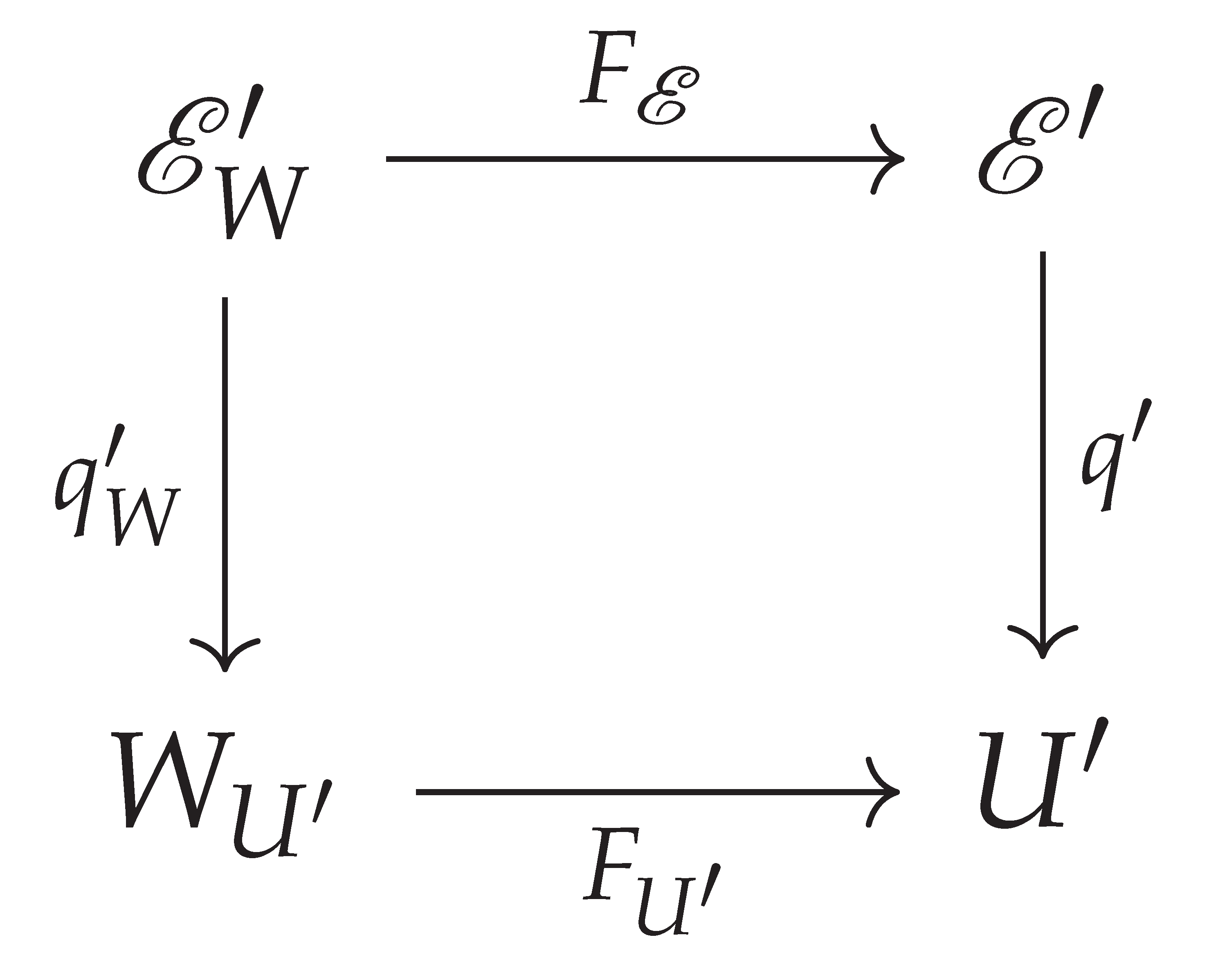 exhibits $q_W^{\prime }$ as finite locally free of degree two, with $R{q}_{W!}^{\prime }\simeq R{q}_{W*}^{\prime }$. For either source coefficient $J_I^{\mathrm{un}}$ or ${\widehat{R}}^{\mathrm{un}}$ in Theorem 9, proper base change gives natural, morphism-compatible isomorphisms 

$$F_{U^{\prime }}^{*}R{q}_{*}^{\prime }J\stackrel{\sim }{\to }R{q}_{W*}^{\prime }{F}_{\mathcal{E}}^{*}J.$$

(195)

 These are comparisons with the base-changed unframed finite map , not an assertion that the unrestricted framed-source map to $U^{\prime }$ is proper or finite. 

Proof. 

Finite locally free morphisms remain finite locally free of the same rank after arbitrary base change. Properness identifies ! and * for $q^{\prime }$ and $q_W^{\prime }$. The square is Cartesian by construction, so proper base change gives (195); its naturality applies to the selected forward morphism and the purity Gysin comparison. The atlas $F_{U^{\prime }}$ is separately smooth and nonproper. □

Lemma 27

(Perverse amplitude under a smooth framing atlas).  Assume the selected stack-theoretic MHM category admits smooth perverse pullback and (191). For $g=g_N$, $n\in \mathbb{Z}$ and $M\in \{I^H,P^H,R_{\mathsf{\Sigma }}^H\}$, 

$$\begin{array}{cc}\hfill {}^p{\mathcal{H}}^{n+g}\left({\mathsf{H}}_{\mathrm{fr}}\left(M\right)\right)& \simeq F_{+}^{*}\left[g\right]{}^p{\mathcal{H}}^n\left({\mathsf{H}}_{\mathrm{un}}\left(M\right)\right).\hfill \end{array}$$

(196)

 The isomorphisms are compatible with transported connecting maps and use the chosen stack normalization. 

Proof. 

For a smooth morphism of relative dimension  g , $F_{+}^{*}\left[g\right]$ is perverse  t -exact. Thus ${}^p{\mathcal{H}}^n\left(F_{+}^{*}K\left[g\right]\right)\simeq F_{+}^{*}\left[g\right]{}^p{\mathcal{H}}^n\left(K\right)$. Reindex the left side as ${}^p{\mathcal{H}}^{n+g}\left(F_{+}^{*}K\right)$ and substitute $K={\mathsf{H}}_{\mathrm{un}}\left(M\right)$ using (191). Naturality proves the compatibility. □

Corollary 9

(Atlas witnesses for the degree-two class).  Assume the compatible equivariant mixed-Hodge normalization of Theorem 9 and Proposition 70. Let $g_{+}$ be the relative dimension of the smooth target atlas $F_{U^{\prime }}$ and set $I_W^{\prime }:=F_{U^{\prime }}^{*}\left[g_{+}\right]I^{\prime }$, $R_W^{\prime }:=F_{U^{\prime }}^{*}\left[g_{+}\right]R^{\prime }$. Then $I_W^{\prime },R_W^{\prime }\in \mathrm{MHM}\left(W_{U^{\prime }}\right)$, and the normalized pullback of the transported connecting arrow is a nonzero class 

$$0\ne F_{U^{\prime }}^{*}\left[g_{+}\right]{ϵ}_{U^{\prime }}\in {\mathrm{Hom}}_{{\mathsf{D}}_H\left(W_{U^{\prime }}\right)}(R_W^{\prime },I_W^{\prime }\left[2\right]).$$

(197)

 Since the atlas $W_{U^{\prime }}$ may be taken to be a quasi-projective variety, $D^H\left(W_{U^{\prime }}\right)=D^b\mathrm{MHM}\left(W_{U^{\prime }}\right)$ is the bounded derived category of its heart, and therefore 

$${\mathrm{Hom}}_{D^H\left(W_{U^{\prime }}\right)}\left(R_W^{\prime },I_W^{\prime }\left[2\right]\right)={\mathrm{Ext}}_{\mathrm{MHM}\left(W_{U^{\prime }}\right)}^2\left(R_W^{\prime },I_W^{\prime }\right);$$

 thus $F_{U^{\prime }}^{*}\left[g_{+}\right]{ϵ}_{U^{\prime }}$ is a nonzero heart-level Yoneda 2-extension on the atlas, even though no such identification is asserted on the stack $U^{\prime }$. Nonvanishing is detected by the specific base-changed purity/Gysin witness; no injectivity of arbitrary derived Hom groups under smooth atlas pullback is asserted. 

Proof. 

Smooth perverse exactness of $F_{U^{\prime }}^{*}\left[g_{+}\right]$, the finite pushforward comparison (195), and the perverse placements of Theorem 9 give the two heart objects and the degree-two type. The node image meets $U^{\prime }$ and the class is represented there by the nonzero codimension-two Gysin scalar. Its pullback on a nonempty smooth chart is the same nonzero scalar on the pulled-back orientation line, proving the inequality. □

Remark 39

(Descent is not ordinary direct image).  The comparison $F_{+}^{*}{\mathsf{H}}_{\mathrm{un}}\simeq {\mathsf{H}}_{\mathrm{fr}}$ is a descent identity, not $R{F}_{+*}{\mathsf{H}}_{\mathrm{fr}}\simeq {\mathsf{H}}_{\mathrm{un}}$. Even for a trivial framing torsor, the latter direct image contains the cohomology of $G_N$. Smooth surjective pullback is conservative on objects but need not be injective on all derived Hom groups. The particular purity/Gysin scalar used on the rank-one branch can nevertheless be tested after nonempty smooth pullback: purity identifies it with a nonzero endomorphism of a constant Tate line. This special detection does not establish faithfulness on unrelated extension classes. 

8.3. First-Jet Information and Its Residual

The intrinsic first-jet quadratic of Proposition 28 has local expression ${\gamma }_1\left(\lambda \right)=c_1+(d_1-a_1)\lambda -b_1{\lambda }^2$. Its descent uses the coordinate transition and gauge action of (47); the following is only an auxiliary line-bundle calculation.

Lemma 28

(The line-bundle forgetting sequence).  For $E={\mathbb{P}}^1$, $\mathcal{S}={\mathcal{O}}_E(-1)$ and $\mathcal{Q}\simeq {\mathcal{O}}_E\left(1\right)$, there is an exact sequence 

$$0⟶{\mathcal{O}}_E(-2)⟶{\mathcal{O}}_E{(-1)}^{\oplus 2}⟶{\mathcal{O}}_E⟶0.$$

(198)

 It induces the smooth affine-line bundle 

$$\varpi :{\mathrm{Tot}}_E({\mathcal{O}}_E{(-1)}^{\oplus 2}\oplus {\mathcal{O}}_E\left(2\right))⟶{\mathrm{Tot}}_E({\mathcal{O}}_E\oplus {\mathcal{O}}_E\left(2\right)),$$

(199)

 whose relative tangent line is the pullback of ${\mathcal{O}}_E(-2)$. This nonproper projection is distinct from the framing atlas $F_{+}$. 

Proof. 

Apply $\mathrm{Hom}(\mathcal{Q},-)$ to the tautological sequence, using $\mathrm{Hom}(\mathcal{Q},\mathcal{S})\simeq {\mathcal{O}}_E(-2)$. The induced fiberwise-surjective map of vector bundles has the stated kernel, so its total-space map is an affine-line bundle. □

Proposition 71

(Self-intersection normalization for a forgotten line).  For a line bundle L on a smooth variety B and its zero section $e:B\hookrightarrow {\mathrm{Tot}}_B\left(L\right)$, 

$$e^{*}{e}_{*}\alpha =c_1\left(L\right)⌣\alpha ,\alpha \in H^{*}(B,\mathbb{Q}).$$

(200)

 Codimension-one purity gives $e^{!}{\mathbb{Q}}_{\mathrm{Tot}L}^H\simeq {\mathbb{Q}}_B^H(-1)[-2]$. For (198), 

$$c_1\left({\mathcal{O}}_E(-2)\right)=-2h\ne 0,h=c_1\left({\mathcal{O}}_E\left(1\right)\right)\in H^2(E,\mathbb{Q}\left(1\right)).$$

(201)

Proof. 

The self-intersection formula identifies the restriction of the Thom–Gysin class with $c_1\left(L\right)$, with the purity twist as stated. For ${\mathcal{O}}_E(-2)$ the first Chern class is $-2h$. □

Remark 40

(Scope of the Euler-class test).  The class $-2h$ measures the auxiliary relative line of (199); it is neither the transported Yoneda arrow nor its normalization. Theorem 8 and its finite-open refinement 9 instead use the genuine kernel-branch inverse and codimension-two purity morphism. 

8.4. The Framing-Defect Cone

The atlas adjunction $F_{+}^{*}⊣R{F}_{+*}$ is distinct from the recollement transformation $j_{!}\to R{j}_{*}$. We work only in a bounded stack-theoretic MHM category supporting the displayed operations.

Definition 31

(Atlas-unit framing residual).  For $T_M={\mathsf{H}}_{\mathrm{un}}\left(M\right)$ and ${\tilde{T}}_M={\mathsf{H}}_{\mathrm{fr}}\left(M\right)$, the natural comparison (191) and the atlas unit give 

$${\eta }_M:T_M⟶R{F}_{+*}{\tilde{T}}_M.$$

(202)

 Define 

$${\mathcal{D}}_F\left(M\right):=\mathrm{Cone}\left({\eta }_M\right)\in {\mathsf{D}}_H\left({\mathcal{Y}}_{+}\right).$$

(203)

Proposition 72

(Exact residual triangle).  The residuals of the corrected forward extension form a distinguished triangle 

$${\mathcal{D}}_F\left(I^H\right)\to {\mathcal{D}}_F\left(P^H\right)\to {\mathcal{D}}_F\left(R_{\mathsf{\Sigma }}^H\right)\stackrel{+1}{\to }.$$

(204)

 For any locally closed immersion $s:Z\hookrightarrow {\mathcal{Y}}_{+}$, restriction gives, in particular, 

$$\begin{array}{cc}\hfill \dots \to {}^p{\mathcal{H}}^n\left(s^{*}{\mathcal{D}}_F\left(I^H\right)\right)& \to {}^p{\mathcal{H}}^n\left(s^{*}{\mathcal{D}}_F\left(P^H\right)\right)\hfill \\ \hfill & \to {}^p{\mathcal{H}}^n\left(s^{*}{\mathcal{D}}_F\left(R_{\mathsf{\Sigma }}^H\right)\right)\hfill \\ \hfill & \to {}^p{\mathcal{H}}^{n+1}\left(s^{*}{\mathcal{D}}_F\left(I^H\right)\right)\to \dots ,\hfill \end{array}$$

(205)

 with the analogous costalk sequence for $s^{!}$. 

Proof. 

Naturality of the unit and $\beta$ gives a morphism from the unframed triangle to $R{F}_{+*}$ of the framed triangle. Its objectwise cones form (204) by the $3\times 3$ lemma; $s^{*}$ and $s^{!}$ give the long exact sequences. □

Lemma 29

(Residual of a locally trivial framing torsor).  If an atlas is locally $\mathrm{pr}:B\times G\to B$ for a connected smooth algebraic group G, then 

$${\mathcal{D}}_F\left(M\right){{|}_B\simeq T_M|}_B\otimes \mathrm{Cone}({\mathbb{Q}}^H\to R\mathsf{\Gamma }{(G,\mathbb{Q})}^H).$$

(206)

 For $G=G{L}_2\left(\mathbb{C}\right)$ this is generally nonzero because $H^1(G,\mathbb{Q})\simeq \mathbb{Q}(-1)$; it need not be supported on the node locus. 

Proof. 

The projection formula identifies $R{\mathrm{pr}}_{*}{\mathrm{pr}}^{*}{T}_M$ with $T_M\otimes R\mathsf{\Gamma }{(G,\mathbb{Q})}^H$; the unit is the tensor product of the identity with ${\mathbb{Q}}^H\to R\mathsf{\Gamma }{(G,\mathbb{Q})}^H$. Taking the cone gives the formula. For $G{L}_2$, the determinant map detects the stated degree-one Tate class. □

Remark 41

(Three different comparison cones).  The atlas-unit residual, the boundary cone of Section 5.4, and the octahedral comparison of Section 6.6 arise from different transformations. None represents the finite-open degree-two derived attachment without a separate morphism-level comparison. 

8.5. Framed Versus Unframed Extension Survival

Theorem 8 gives the nonzero  unframed  unit-kernel target arrow. We record its framed witnesses and a general detection criterion for other kernels; neither asserts generic faithfulness of smooth-atlas pullback.

Theorem 11

(Extension detection under verified framing descent).  Under Proposition 68, let ${ϵ}_{\mathrm{fr}}$ and ${ϵ}_{\mathrm{un}}$ denote the connecting maps in (192). Then: 

(i)

 If ${ϵ}_{\mathrm{fr}}\ne 0$, then ${ϵ}_{\mathrm{un}}\ne 0$ and the unframed derived extension triangle is nonsplit. 

(ii)

 If 

$$\begin{array}{cc}\hfill {\mathrm{Hom}}_{{\mathsf{D}}_H\left({\mathcal{Y}}_{+}\right)}(T_{R_{\mathsf{\Sigma }}^H},T_{I^H}\left[1\right])⟶& \\ \hfill & {\mathrm{Hom}}_{{\mathsf{D}}_H\left(W_{+}^{\mathrm{fr}}\right)}(F_{+}^{*}{T}_{R_{\mathsf{\Sigma }}^H},F_{+}^{*}{T}_{I^H}\left[1\right])\hfill \end{array}$$

(207)

 is injective, then ${ϵ}_{\mathrm{fr}}=0$ if and only if ${ϵ}_{\mathrm{un}}=0$. 

(iii)

 If the transported unframed endpoints lie in $\mathrm{MHM}\left({\mathcal{Y}}_{+}\right)$, the connecting morphism is the Yoneda class of the resulting short exact sequence; otherwise it remains a derived morphism with potentially higher Postnikov attachments. 

Proof. 

By (192), ${\beta }_{I^H}\left[1\right]\circ F_{+}^{*}{ϵ}_{\mathrm{un}}={ϵ}_{\mathrm{fr}}\circ {\beta }_{R_{\mathsf{\Sigma }}^H}$. Hence ${ϵ}_{\mathrm{un}}=0$ implies ${ϵ}_{\mathrm{fr}}=0$, proving (i) by contraposition and the derived splitting criterion of Lemma 22. Under the injectivity assumption, $F_{+}^{*}{ϵ}_{\mathrm{un}}=0$ implies ${ϵ}_{\mathrm{un}}=0$, proving (ii). For (iii), extension closure of the perverse heart converts the transported triangle into a short exact sequence whenever its endpoints lie in that heart; otherwise perverse truncation does not determine the connecting map from its graded pieces. The injectivity in (ii) is not inferred merely from smooth surjectivity of $F_{+}$. □

Corollary 10

(Detection by a normalized local Gysin map).  Assume Theorem 11. If a specified geometric restriction of the actual framed target arrow ${ϵ}_{\mathrm{fr}}$ is identified by base change and purity with a nonzero Gysin morphism, then the unframed extension triangle is nonsplit. The nonzero pre-target class of Proposition 49, or a nonzero multiple of $-2h$ from (201), supplies such a test only after its image under the actual modified-Higgs pushforward is identified with that restriction. 

Proof. 

A functor maps a zero morphism to zero, so a nonzero restriction implies ${ϵ}_{\mathrm{fr}}\ne 0$. Theorem 11(i) gives ${ϵ}_{\mathrm{un}}\ne 0$. The stated identification is necessary because the incidence pullback, auxiliary Euler class, and target pushforward are distinct morphisms.

□

Corollary 11

(Localized nonvanishing and compatible framing witnesses).  Assume the hypotheses of Theorem 8, including its unit kernel and selected equivariant mixed-Hodge normalization. Let U be its nonempty admissible rank-one open. Then the unframed ordinary and exceptional target extension triangles are derived nonsplit on U. On any compatible nonempty smooth framing atlas $F_U:W_U\to U$ as in Proposition 69, the corresponding normalized framed target morphisms are also nonzero: 

$$F_U^{*}{ϵ}_{+,*}{{|}_U\ne 0,F_U^{*}{ϵ}_{+,!}|}_U\ne 0.$$

(208)

 This is a detection of the particular geometric purity class; it does not assert that $F_U^{*}$ is injective on every derived Hom group. 

Proof. 

Nonvanishing of the two unframed arrows is (163). The proof of Theorem 8 detects them by a nonzero codimension-two Gysin morphism on the kernel branch. By (193), the branch isomorphism is preserved after pullback to $W_U$; smooth base change preserves the regular immersion and the purity adjoint. On a nonempty smooth chart, that adjoint is the same nonzero scalar endomorphism of the Tate orientation line, so the framed images are nonzero. Naturality of (192) identifies them with the displayed pullbacks, up to the agreed common smooth normalization. □

Remark 42

(General kernels and the remaining descent problem).  The rank-one inverse is geometric, but survival is proved for the unit kernel with the selected equivariant costalk generator. Other kernels, unrelated nodal sources, and convolution require independent coefficient and Gysin comparisons. Theorem 9 supplies the exceptional unit-kernel case in which the target’s shifted quotient and intersection-complex terms are perverse on $U^{\prime }$, giving a degree-two derived attachment. It does not assert that the unshifted quotient lies in the perverse heart, or extend to arbitrary kernels. 

Remark 43

(Global status of the framing comparison).  For the selected unit-kernel universal coefficient, localized actual target nonvanishing is established in Theorem 8; Corollary 11 records its compatible framed witnesses. Theorem 11 remains the general detection statement when an independent framed target calculation is available. Over the saturated finite open $U^{\prime }$, Proposition 70 and Corollary 9 additionally identify the framed witness and its precise degree-two placement. The remaining perverse and Postnikov questions concern the complement of $U^{\prime }$, arbitrary kernels, and independently realized global nodal sources. The atlas-unit residual and auxiliary jet Euler class remain separate from the forward Yoneda morphism. 

9. Specialization and Bounded Hecke Convolution

We compare specialization in a degeneration parameter with composition of elementary Hecke modifications, always on specified coefficient diagrams. The Springer overlap is a transverse slice of bounded two-step $G{L}_2$ affine-Grassmannian convolution; the explicit lattice model distinguishes the pure Springer ${\mathbb{Q}}^H(-1)$ summand from the corrected forward quotient ${\mathbb{Q}}^H(-2)$. The composition and nearby-cycle identities below require their own proper kernel, base-change, and family-exchange hypotheses. In particular, finiteness of the single-step unframed correspondence over $U^{\prime }$ (Proposition 59) does not by itself provide a collision family or a two-stage convolution theorem. We write  s  for the degeneration parameter,  w  for the Hecke-point parameter, and $\tau$ for a possible collision parameter.

9.1. Family-Level Hecke Correspondence

We use the conventions of Section 1.6. Put $S={\mathbb{A}}_s^1$ and let $i_S:\left\{0\right\}\hookrightarrow S$. The parameters $s,w,\tau$ remain independent unless an explicit base change identifies them.

Definition 32

(Admissible Hecke family).  A specialization-admissible framed Hecke family consists of finite-type complex algebraic spaces, or quotient charts on which the required mixed-Hodge-module operations are defined, fitting into a commutative diagram over S, 

(209)

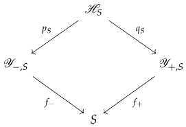
 The structure map $h_S:{\mathcal{H}}_S\to S$ is the common composite $f_{-}{p}_S=f_{+}{q}_S$. Write 

$$\begin{array}{c}{\mathcal{H}}_0={\mathcal{H}}_S{\times }_S\left\{0\right\},{\mathcal{Y}}_{\pm ,0}={\mathcal{Y}}_{\pm ,S}{\times }_S\left\{0\right\},\\ {\iota }_H:{\mathcal{H}}_0\hookrightarrow {\mathcal{H}}_S,{\iota }_{\pm }:{\mathcal{Y}}_{\pm ,0}\hookrightarrow {\mathcal{Y}}_{\pm ,S}.\end{array}$$

 The datum is required to satisfy: 

•  $q_S$ is proper on the selected correspondence support, so its ordinary and exceptional direct images agree there; 
•  the squares with ${\iota }_H$, ${\iota }_{-}$, ${\iota }_{+}$ are Cartesian; 
•  the pullback comparison for $p_S$ and the specialization comparison for the correspondence kernel exist in $D^b\mathrm{MHM}$ and are isomorphisms on the selected coefficients; 
•  the chosen source-to-Hecke realization is defined over S and respects these specialization comparisons. 

 For example, smoothness of $p_S$ provides the required comparison between nearby cycles and pullback, with the appropriate perverse shifts. Condition (F3) is not imposed automatically on arbitrary singular incidence spaces. 

A nonproper correspondence can be treated with $R{q}_{S!}$ only after its own compact-support specialization exchanges and boundedness conditions have been verified; this variant is not identified with the ordinary-image construction below.

The Cartesian squares used below are, for either sign,

(210)

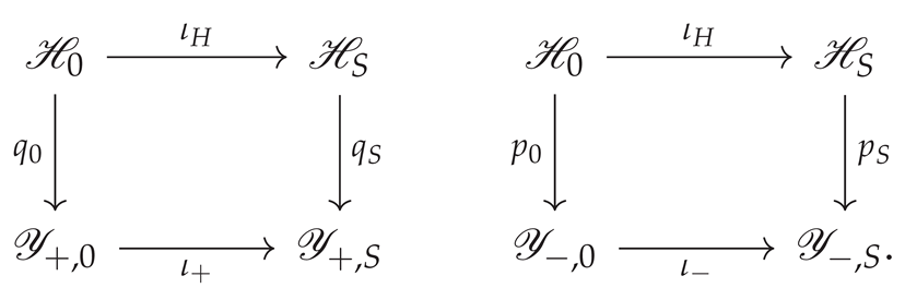
Their Cartesian property follows from the equality of the structure maps to  S , not from a similarity of completed local equations.

Definition 33

(Family transport and specialization comparison).  Fix ${\mathcal{K}}_S\in D^b\mathrm{MHM}\left({\mathcal{H}}_S\right)$, a cohomological shift $d\in \mathbb{Z}$, and a Tate twist $m\in \mathbb{Z}$. On the chosen bounded domain define 

$${\mathsf{H}}_S\left(M\right)=R{q}_{S*}\left(p_S^{*}M\otimes {\mathcal{K}}_S\right)\left[d\right]\left(m\right),$$

(211)

 with ${\mathsf{H}}_0$ defined using $p_0,q_0$ and the specified specialization ${\mathcal{K}}_0$ of the kernel. The operations in (211) are assumed to preserve the chosen bounded constructible subcategory. A specialization comparison consists of natural isomorphisms, for $\diamond \in \{\mathsf{\Psi },\mathsf{\Phi }\}$, 

$${\beta }_{\diamond ,M}:{\mathsf{H}}_0\left({\diamond }_{f_{-}}^{H}M\right)\stackrel{\sim }{\to }{\diamond }_{f_{+}}^H\left({\mathsf{H}}_S\left(M\right)\right),$$

(212)

 compatible with canonical and variation morphisms and with the Tate twist $(-1)$. 

Proposition 73

(Construction from proper base change).  Assume Definition 32, and suppose that for each selected M the exchange maps 

$$\begin{array}{cc}\hfill {\diamond }_{h_S}^H(p_S^{*}M\otimes {\mathcal{K}}_S)& \stackrel{\sim }{\leftarrow }{p}_0^{*}\left({\diamond }_{f_{-}}^{H}M\right)\otimes {\mathcal{K}}_0,\hfill \\ \hfill {\diamond }_{f_{+}}^{H}R{q}_{S*}(-)& \stackrel{\sim }{\to }R{q}_{0*}{\diamond }_{h_S}^H(-)\hfill \end{array}$$

 are given, for $\diamond =\mathsf{\Psi },\mathsf{\Phi }$, with the normalization of (211). Then the inverses and composites of these exchanges define (212). 

Proof. 

Apply the first exchange map to  M . Next apply the exact functor $R{q}_{0*}\left[d\right]\left(m\right)$. This gives an isomorphism from ${\mathsf{H}}_0\left({\diamond }_{f_{-}}^{H}M\right)$ to $R{q}_{0*}{\diamond }_{h_S}^H(p_S^{*}M\otimes {\mathcal{K}}_S)\left[d\right]\left(m\right)$. The inverse of proper specialization for $q_S$ identifies this last object with ${\diamond }_{f_{+}}^H{\mathsf{H}}_S\left(M\right)$. Every arrow is natural in  M . Thus the composite is a natural isomorphism. The statement involves the specified kernel exchange: proper base change for $q_S$ alone does not supply the first arrow [3,25,27]. □

Remark 44

(What the family construction does not supply).  The determinant family and its smooth evaluation pullback supply a Cartesian invariant-line family, but they do not automatically supply a proper modified-Higgs target projection or a specialization-compatible kernel. The single-step finite morphism $q^{\prime }$ on $U^{\prime }$ of Proposition 59 proves properness only after restriction to that open ; it does not extend the properness assumption (F1) over a family, nor furnish the exchange (F3). The identities below apply only when those separate hypotheses hold. 

9.2. Compatibility with Canonical and Variation Maps

Let  M  be a coefficient on ${\mathcal{Y}}_{-,S}$ for which (212) is defined. Put

$$\begin{array}{cc}{\mathsf{\Psi }}_{-}^H\left(M\right)={\psi }_{f_{-},1}^H\left(M\right),\hfill & {\mathsf{\Phi }}_{-}^H\left(M\right)={\varphi }_{f_{-},1}^H\left(M\right),\hfill \\ {\mathsf{\Psi }}_{+}^H\left({\mathsf{H}}_{S}M\right)={\psi }_{f_{+},1}^H\left({\mathsf{H}}_{S}M\right),\hfill & {\mathsf{\Phi }}_{+}^H\left({\mathsf{H}}_{S}M\right)={\varphi }_{f_{+},1}^H\left({\mathsf{H}}_{S}M\right).\hfill \end{array}$$

The canonical and variation arrows have types

$${\mathrm{can}}_{\pm }^H:{\mathsf{\Psi }}_{\pm }^H⟶{\mathsf{\Phi }}_{\pm }^H,{\mathrm{Var}}_{\pm }^H:{\mathsf{\Phi }}_{\pm }^H⟶{\mathsf{\Psi }}_{\pm }^H(-1).$$

Proposition 74

(Tate-typed naturality).  Under the hypotheses of Proposition 73, the diagrams 

(213)

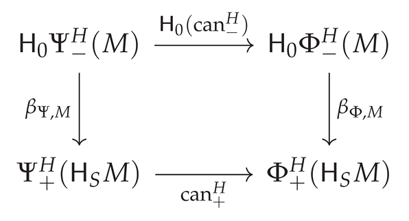 and 

(214)

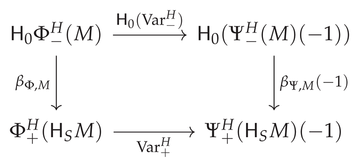 commute. Consequently, with $N_{\pm }^H={\mathrm{Var}}_{\pm }^H\circ {\mathrm{can}}_{\pm }^H$, 

$${\beta }_{\mathsf{\Psi },M}(-1)\circ {\mathsf{H}}_0\left(N_{-}^H\right)=N_{+}^H\circ {\beta }_{\mathsf{\Psi },M}.$$

(215)

Proof. 

The two comparisons ${\beta }_{\mathsf{\Psi },M}$ and ${\beta }_{\mathsf{\Phi },M}$ are composites of functorial exchange morphisms. The transformations ${\mathrm{can}}^H$ and ${\mathrm{Var}}^H$ are natural for proper direct image and for the stipulated pullback and kernel exchange. Applying naturality to each component of the composite shows that the two routes around (213) agree. The same argument for variation gives (214); its right-hand side is ${\mathsf{\Psi }}_{+}^H\left({\mathsf{H}}_{S}M\right)(-1)$, not the untwisted nearby cycle object. Composing the two commutative squares gives (215), since derived pull–push and the kernel construction commute with Tate twisting [3,25,27]. □

Remark 45

(The two node-supported channels).  The application of ${\mathsf{H}}_0$ to the forward extension $R_{\mathsf{\Sigma }}^H\stackrel{{ϵ}_{\mathsf{\Sigma }}}{\to }{I}^H\left[1\right]$ and to the factorization ${\mathsf{\Psi }}^H\stackrel{u_{\mathsf{\Sigma }}}{\to }{Q}_{\mathsf{\Sigma }}^H\stackrel{v_{\mathsf{\Sigma }}}{\to }{\mathsf{\Psi }}^H(-1)$ produces two distinct diagrams. The objects $R_{\mathsf{\Sigma }}^H$ and $Q_{\mathsf{\Sigma }}^H$ have respective Tate factors ${\mathbb{Q}}^H(-2)$ and ${\mathbb{Q}}^H(-1)$. The squares above preserve the variation type, but do not identify these two images or their maps. Such an identification would require a separate morphism between the corresponding transported diagrams. 

9.3. Two Successive Elementary Hecke Modifications

Definition 34

(Two-stage correspondence and kernels).  Let $Y_0,Y_1,Y_2$ be specified finite-type moduli charts (or quotient stacks with an available bounded MHM formalism). For $i=1,2$ fix correspondences 

$$Y_{i-1}\stackrel{p_i}{\leftarrow }{\mathcal{H}}_i\stackrel{q_i}{\to }{Y}_i$$

 and kernels ${\mathcal{K}}_i\in D^b\mathrm{MHM}\left({\mathcal{H}}_i\right)$. Assume the fiber product 

$${\mathcal{H}}_{12}:={\mathcal{H}}_1{\times }_{Y_1}{\mathcal{H}}_2$$

 is defined in the chosen category and write ${\rho }_i:{\mathcal{H}}_{12}\to {\mathcal{H}}_i$ for its projections. Set 

$$p_{12}=p_1{\rho }_1,q_{12}=q_2{\rho }_2,{\mathcal{K}}_{12}={\rho }_1^{*}{\mathcal{K}}_1\otimes {\rho }_2^{*}{\mathcal{K}}_2.$$

 Suppose also that there is a proper map $m:{\mathcal{H}}_{12}\to {\mathcal{H}}_{21}$ to a bounded terminal correspondence, with maps $p_{21},q_{21}$ satisfying 

$$p_{21}m=p_{12},q_{21}m=q_{12}.$$

 The convolution kernel on the terminal correspondence is 

$${\mathcal{K}}_{21}:=R{m}_{*}{\mathcal{K}}_{12},$$

(216)

 when this derived image is bounded and constructible. All cohomological shifts and Tate twists of the kernels are included in the chosen normalizations of ${\mathcal{K}}_i$. 

Proposition 75

(Composition as derived convolution).  Assume that $q_1,q_2,m$ are proper on the relevant supports, and that proper base change and projection formula apply to the displayed correspondences and kernels. Set 

$${\mathsf{H}}_i\left(F\right)=R{q}_{i*}(p_i^{*}F\otimes {\mathcal{K}}_i),{\mathsf{H}}_{21}\left(F\right)=R{q}_{21*}(p_{21}^{*}F\otimes {\mathcal{K}}_{21}).$$

 Then there is a natural isomorphism of exact derived functors 

$$\mathsf{\Theta }:{\mathsf{H}}_2\circ {\mathsf{H}}_1\stackrel{\sim }{\to }{\mathsf{H}}_{21}$$

(217)

 on the specified bounded coefficient category. This assertion does not imply perverse t-exactness of either side. 

Proof. 

Let $F\in D^b\mathrm{MHM}\left(Y_0\right)$ be in the specified domain. By definition,

$$\begin{array}{cc}\hfill {\mathsf{H}}_2{\mathsf{H}}_1\left(F\right)& =R{q}_{2*}\left(p_2^{*}R{q}_{1*}(p_1^{*}F\otimes {\mathcal{K}}_1)\otimes {\mathcal{K}}_2\right).\hfill \end{array}$$

The square

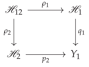is Cartesian. Proper base change changes $p_2^{*}R{q}_{1*}$ into $R{\rho }_{2*}{\rho }_1^{*}$. The projection formula for ${\rho }_2$ then gives

$$\begin{array}{cc}\hfill {\mathsf{H}}_2{\mathsf{H}}_1\left(F\right)& \simeq R{q}_{2*}R{\rho }_{2*}\left({\rho }_1^{*}{p}_1^{*}F\otimes {\rho }_1^{*}{\mathcal{K}}_1\otimes {\rho }_2^{*}{\mathcal{K}}_2\right)\hfill \\ & =R{q}_{12*}(p_{12}^{*}F\otimes {\mathcal{K}}_{12}).\hfill \end{array}$$

Since $q_{12}=q_{21}m$, the last expression is $R{q}_{21*}R{m}_{*}(m^{*}{p}_{21}^{*}F\otimes {\mathcal{K}}_{12})$. Applying the projection formula for the proper map  m  gives

$$R{q}_{21*}\left(p_{21}^{*}F\otimes R{m}_{*}{\mathcal{K}}_{12}\right)={\mathsf{H}}_{21}\left(F\right).$$

All equivalences are induced by canonical six-functor transformations and are natural in  F . Their composite defines $\mathsf{\Theta }$. Every functor used is exact on distinguished triangles; no perverse-heart exactness has been invoked. □

Remark 46

(Associativity and the bounded domain).  The fixed-point lattice chain does not itself supply a family over a collision parameter τ. Such a family requires the appropriate Beilinson–Drinfeld (or equivalent) configuration-space geometry, together with specialization-compatible kernels. For three modifications, the associator is obtained from the coherent projection-formula and base-change transformations in an enhanced six-functor setting. Equation (217) is about the selected bounded kernel category. The finite degree-two map over $U^{\prime }$ is a single-step restriction, and does not establish the properness or kernel exchange needed for two-step composition. Neither pure Satake semisimplicity nor this finite-open result supplies a convolution action on arbitrary mixed-Hodge extensions. 

9.4. Octahedral Coherence Under Hecke Composition

Let $u:A_0\to A_1$ and $v:A_1\to A_2$ be composable morphisms on one terminal space  Y . In a fixed stable enhancement put $D_u=\mathrm{Cone}\left(u\right)$, $D_v=\mathrm{Cone}\left(v\right)$ and $D_{vu}=\mathrm{Cone}\left(vu\right)$.

Lemma 30

(Octahedral comparison).  The standard octahedral triangle is 

$$D_u⟶D_{vu}⟶D_v\stackrel{{\omega }_{u,v}}{\to }{D}_u\left[1\right].$$

(218)

 For an exact enhanced functor T, the induced cofiber identifications are compatible with its connecting arrow: 

$$T\left({\omega }_{u,v}\right)={\omega }_{T\left(u\right),T\left(v\right)}.$$

(219)

 The equality uses the chosen coherent cone identifications. 

Proof. 

Take chain representatives of $u,v$. The cone maps are induced by $(b,a)\mapsto (vb,a)$ and $(c,a)\mapsto (c,ua)$; with the cohomological cone convention the third arrow is $(c,b^{\prime })\mapsto (b^{\prime },0)$ into $D_u\left[1\right]$. Their chain-map identities and the null-homotopy of the first composite are checked in Appendix C. Exactness of  T  preserves this cofiber diagram, hence the connecting map as well. □

Proposition 76

(Octahedra under convolution comparison).  For the natural equivalence $\mathsf{\Theta }:{\mathsf{H}}_2{\mathsf{H}}_1\Rightarrow {\mathsf{H}}_{21}$ of Proposition 75, one has 

$$\begin{array}{cc}\hfill {\mathsf{\Theta }}_{A_2}{\mathsf{H}}_2{\mathsf{H}}_1\left(vu\right)& ={\mathsf{H}}_{21}\left(vu\right){\mathsf{\Theta }}_{A_0},\hfill \\ \hfill {\mathsf{\Theta }}_{D_u}\left[1\right]{\mathsf{H}}_2{\mathsf{H}}_1\left({\omega }_{u,v}\right)& ={\mathsf{H}}_{21}\left({\omega }_{u,v}\right){\mathsf{\Theta }}_{D_v}.\hfill \end{array}$$

(220)

 These are identities of coefficient-cone maps, not statements about the value of the forward Yoneda morphism. 

Proof. 

Naturality of $\mathsf{\Theta }$ gives the first identity for $vu$ and the second for ${\omega }_{u,v}$. Lemma 30 supplies the coherent identifications of the two transported octahedra. □

Remark 47

(Composition defect versus Yoneda class).  The morphisms ${\omega }_{u,v}:D_v\to D_u\left[1\right]$ and ${ϵ}_{\mathsf{\Sigma }}:R_{\mathsf{\Sigma }}^H\to I^H\left[1\right]$ have different sources and targets; vanishing of one does not imply vanishing of the other. This distinction also occurs in the local Hecke-collision calculations of [37]. 

9.5. Affine-Grassmannian Realization and Convolution

Put $\mathcal{O}=\mathbb{C}\left[\right[w\left]\right]$, $\mathcal{K}=\mathbb{C}\left(\right(w\left)\right)$, $V={\mathbb{C}}^2$ and ${\mathsf{\Lambda }}_0=\mathcal{O}{\otimes }_{\mathbb{C}}V$. Write $\mathrm{Gr}=G{L}_2\left(\mathcal{K}\right)/G{L}_2\left(\mathcal{O}\right)$ and use upper modifications for the lattice chain. Their relation with the lower Hecke convention of Definition 6 is inversion of the lattice inclusion, not an identification of the two oriented correspondences.

Proposition 77

(Minuscule lattice correspondence).  For a line $\ell \subset V={\mathsf{\Lambda }}_0/w{\mathsf{\Lambda }}_0$, let $\tilde{\ell }\subset {\mathsf{\Lambda }}_0$ be its inverse image and define 

$${\mathsf{\Lambda }}_{\ell }^{\prime }={\mathsf{\Lambda }}_0+w^{-1}\tilde{\ell }=w^{-1}\tilde{\ell }.$$

(221)

 Then ${\mathsf{\Lambda }}_0\subset {\mathsf{\Lambda }}_{\ell }^{\prime }\subset w^{-1}{\mathsf{\Lambda }}_0$ with ${\dim }_{\mathbb{C}}({\mathsf{\Lambda }}_{\ell }^{\prime }/{\mathsf{\Lambda }}_0)=1$. These lattices form the minuscule Schubert variety ${\mathrm{Gr}}^{\le (1,0)}\simeq \mathbb{P}\left(V\right)$. The construction raises the degree by one. 

Proof. 

Modulo ${\mathsf{\Lambda }}_0$, the lattice in (221) is precisely the line $w^{-1}\ell \subset w^{-1}{\mathsf{\Lambda }}_0/{\mathsf{\Lambda }}_0\simeq V$; conversely every such intermediate lattice determines a unique line. This is an isomorphism of projective moduli functors. The quotient has length one, fixing the relative coweight and degree change [9]. □

Proposition 78

(Bounded two-step lattice convolution).  The moduli space $\mathcal{C}$ of chains 

$${\mathsf{\Lambda }}_0\subset {\mathsf{\Lambda }}_1\subset {\mathsf{\Lambda }}_2,{\dim }_{\mathbb{C}}({\mathsf{\Lambda }}_i/{\mathsf{\Lambda }}_{i-1})=1,$$

(222)

 with each quotient annihilated by w, is the convolution variety ${\mathrm{Gr}}^{\le (1,0)}\tilde{\times }{\mathrm{Gr}}^{\le (1,0)}$. The terminal-lattice map $m_{21}:\mathcal{C}\to \mathcal{S}:={\mathrm{Gr}}^{\le (2,0)}$ is projective, birational, and semismall. The stratum $(1,1)$ is the single point ${\mathsf{\Lambda }}_{*}:=w^{-1}{\mathsf{\Lambda }}_0$. 

Proof. 

For each first lattice ${\mathsf{\Lambda }}_1$, the second step is parametrized by the lines in ${\mathsf{\Lambda }}_1/w{\mathsf{\Lambda }}_1$; hence $\mathcal{C}$ is a projective-line bundle over ${\mathbb{P}}^1$. The terminal lattice has length two over ${\mathsf{\Lambda }}_0$, with elementary divisors either $(2,0)$ or $(1,1)$. The first case is open dense and determines the unique intermediate lattice ${\mathsf{\Lambda }}_1={\mathsf{\Lambda }}_0+w{\mathsf{\Lambda }}_2$; the second case has terminal lattice ${\mathsf{\Lambda }}_{*}$. Thus $m_{21}$ is birational, with exceptional fiber ${\mathbb{P}}^1$ over a codimension-two point, and is semismall. Properness follows from the relative projective flag construction [9,10]. □

Lemma 31

(The exceptional minuscule convolution fiber).  The fiber $m_{21}^{-1}\left({\mathsf{\Lambda }}_{*}\right)$ parametrizes all lines in ${\mathsf{\Lambda }}_{*}/{\mathsf{\Lambda }}_0\simeq V$ and is ${\mathbb{P}}^1$. Its cohomology is $H^0({\mathbb{P}}^1,\mathbb{Q})=\mathbb{Q}$ and $H^2({\mathbb{P}}^1,\mathbb{Q})=\mathbb{Q}(-1)$. 

Proof. 

An intermediate ${\mathsf{\Lambda }}_1$ is the inverse image of a line in ${\mathsf{\Lambda }}_{*}/{\mathsf{\Lambda }}_0$; both successive quotients are then annihilated by  w . This identifies the fiber scheme with the projective line. The Hodge cohomology follows from the projective bundle formula. □

Proposition 79

(Nilpotent matrix chart in the convolution slice).  Let $\mathcal{N}=\{A\in \mathfrak{sl}(V):\det A=0\}$ and put ${\mathsf{\Lambda }}_{*}=w^{-1}{\mathsf{\Lambda }}_0$. For $A\in \mathcal{N}$ set 

$${\mathsf{\Lambda }}_A=(1+w^{-1}A){\mathsf{\Lambda }}_{*}.$$

(223)

 Then ${\mathsf{\Lambda }}_0\subset {\mathsf{\Lambda }}_A\subset w^{-2}{\mathsf{\Lambda }}_0$, and ${\mathsf{\Lambda }}_A/{\mathsf{\Lambda }}_0$ has length two. Moreover, 

$$\begin{array}{cc}\hfill {\tau }_A:V& ⟶{\mathsf{\Lambda }}_A/{\mathsf{\Lambda }}_0,\hfill \\ \hfill v& ⟼w^{-1}v+w^{-2}Av\left(\mathrm{mod}{\mathsf{\Lambda }}_0\right)\hfill \end{array}$$

(224)

 is a $\mathbb{C}$-linear isomorphism such that $w{\tau }_A\left(v\right)={\tau }_A\left(Av\right)$. The assignment $A\mapsto {\mathsf{\Lambda }}_A$ identifies $\mathcal{N}$ with the $A_1$ transverse affine-Grassmannian slice through ${\mathsf{\Lambda }}_{*}$, with its reduced scheme structure. 

Proof. 

Cayley–Hamilton gives $A^2=0$, whence ${(1+w^{-1}A)}^{-1}=1-w^{-1}A$ and $\det (1+w^{-1}A)=1$. For $x\in {\mathsf{\Lambda }}_0$, the vector $(1-w^{-1}A)x$ belongs to ${\mathsf{\Lambda }}_{*}$, proving ${\mathsf{\Lambda }}_0\subset {\mathsf{\Lambda }}_A$; the other inclusion is immediate. The determinant has valuation $-2$, so ${\mathsf{\Lambda }}_A/{\mathsf{\Lambda }}_0$ has length two. Every class has a representative $w^{-1}v+w^{-2}Av$; reduction first modulo $w^{-2}$ and then $w^{-1}$ shows injectivity of (224). Finally,

$$w{\tau }_A\left(v\right)=v+w^{-1}Av\equiv {\tau }_A\left(Av\right)\left(\mathrm{mod}{\mathsf{\Lambda }}_0\right).$$

The inverse graph chart recovers  A  from the action of  w  on the marked quotient. The scheme-level slice identification is the type- A  result of [10]. The preceding calculation gives its rank-two formula. □

Theorem 12

(Springer overlap as a convolution slice).  The base change of $m_{21}$ along $\mathcal{N}\hookrightarrow \mathcal{S}$ identifies with the Springer resolution from Proposition 17: 

(225)

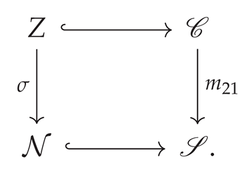
 Here $Z=\{(A,\ell ):\mathrm{im}A\subseteq \ell \subseteq \ker A\}\simeq {\mathrm{Tot}}_{{\mathbb{P}}^1}\mathcal{O}(-2)$. The square is Cartesian as a diagram of the specified reduced transverse-slice and relative elementary-modification schemes, not merely on closed points. 

Proof. 

For $A\in \mathcal{N}$, the quotient $M_A:={\mathsf{\Lambda }}_A/{\mathsf{\Lambda }}_0$ is identified with  V  through ${\tau }_A$, and  w  acts by  A . An intermediate lattice corresponds to a line subbundle $L={\mathsf{\Lambda }}_1/{\mathsf{\Lambda }}_0\subset M_A$, hence to $\ell ={\tau }_A^{-1}\left(L\right)\subset V$. The first step is an elementary modification of type $(1,0)$ precisely when $wL=0$, i.e. $A\ell =0$. The second step is elementary precisely when $w(M_A/L)=0$, i.e. $\mathrm{im}A\subseteq \ell$. Both conditions are necessary over arbitrary base schemes; requiring mere  A -invariance of  ℓ  would give a potentially larger nonreduced incidence functor. Conversely the two containments define an $\mathcal{O}$-stable intermediate lattice with both prescribed elementary quotients. These constructions commute with base change and are inverse on relative flag functors; together with Proposition 79 they give the stated Cartesian square. For fixed  ℓ , the matrices factor as $V/\ell \to \ell$, giving $\mathrm{Hom}(V/\ell ,\ell )\simeq {\mathcal{O}}_{{\mathbb{P}}^1}(-2)$. The resulting map to $\mathcal{N}$ is exactly $\sigma$. □

Corollary 12

(The Springer Tate summand in two-step convolution).  The pure convolution direct image is 

$$R{m}_{21*}{\mathbb{Q}}_{\mathcal{C}}^H\left[2\right]\simeq {\mathrm{IC}}_{\mathcal{S}}^H\oplus i_{{\mathsf{\Lambda }}_{*}*}{\mathbb{Q}}_{\left\{{\mathsf{\Lambda }}_{*}\right\}}^H(-1).$$

(226)

 Restriction to the slice recovers $R{\sigma }_{*}{\mathbb{Q}}_Z^H\left[2\right]\simeq {\mathrm{IC}}_{\mathcal{N}}^H\oplus i_{o*}{\mathbb{Q}}^H(-1)$ of Proposition 18. The point-supported summand corresponds, under geometric Satake, to the determinant summand in $V_{(1,0)}^{\otimes 2}\simeq V_{(2,0)}\oplus V_{(1,1)}$; it is not the source forward quotient of Tate type ${\mathbb{Q}}^H(-2)$. 

Proof. 

The map $m_{21}$ is proper semismall and generically one-to-one. The semismall decomposition theorem gives the open intersection-complex summand and one point-supported summand, whose stalk multiplicity and pure Tate twist are fixed by $H^2(m_{21}^{-1}\left({\mathsf{\Lambda }}_{*}\right),\mathbb{Q})=\mathbb{Q}(-1)$. Proper base change along the Cartesian square (225) gives the Springer decomposition, with no extra shift because both target slices have dimension two. Geometric Satake identifies the two perverse supports with the symmetric-square and determinant representations in the standard tensor square [9,21]. A decomposition isomorphism is provided by purity; it is not used to declare a canonical coefficient projector or a morphism to the source ${ϵ}_{\mathsf{\Sigma }}$. □

Lemma 32

(The compact convolution surface).  The two-step convolution space is a projective Hirzebruch surface $\mathcal{C}\simeq {\mathbb{P}}_{{\mathbb{P}}^1}(\mathcal{O}\left(1\right)\oplus \mathcal{O}(-1))\simeq {\mathbb{F}}_2$. Its Springer inverse-image slice is a nonproper open surface $Z\simeq {\mathrm{Tot}}_{{\mathbb{P}}^1}\mathcal{O}(-2)$, not the whole convolution variety. 

Proof. 

The first lattice is indexed by $\ell \in \mathbb{P}\left(V\right)$. The rank-two vector bundle ${\mathsf{\Lambda }}_1/w{\mathsf{\Lambda }}_1$ fits in

$$0\to V/\ell \simeq \mathcal{O}\left(1\right)\to {\mathsf{\Lambda }}_1/w{\mathsf{\Lambda }}_1\to \ell \simeq \mathcal{O}(-1)\to 0.$$

Its extension class belongs to $H^1({\mathbb{P}}^1,\mathcal{O}\left(2\right))=0$, so it splits, not canonically. Its line projectivization is ${\mathbb{F}}_2$. Under such a splitting the complement of the section associated with the $\mathcal{O}(-1)$ summand is $\mathrm{Tot}\mathcal{O}(-2)$; the slice theorem identifies this open subset independently of the chosen splitting. □

Remark 48

(Equivariance and extensions in Satake categories).  The pure spherical Hodge-Satake category is semisimple, so its heart-level ${\mathrm{Ext}}^1$ cannot retain an arbitrary nonsplit mixed extension. The calculation above identifies the geometric origin of the ${\mathbb{Q}}^H(-1)$ convolution summand, not the image of ${ϵ}_{\mathsf{\Sigma }}$. An extension-sensitive comparison must be made in the specified mixed or derived category with its equivariance and proper kernel maps [21,25,26]. 

9.6. Extension-Sensitive Bounded Fusion Theorem

Let

$$I^H⟶P^H⟶R_{\mathsf{\Sigma }}^H\stackrel{{ϵ}_{\mathsf{\Sigma }}}{\to }{I}^H\left[1\right]$$

(227)

be the corrected forward triangle of Section 2.2. We take it as a specified object of the derived category of exact diagrams; all functors below act on the maps as well as their endpoints.

Theorem 13

(Bounded fusion of the selected extension diagram).  Assume the following data and hypotheses. 

(H1)

 The geometric source realization of (227) into $D^b\mathrm{MHM}\left(Y_0\right)$ is constructed and fixed, with its forward Yoneda morphism. 

(H2)

 The two Hecke correspondences, the kernels ${\mathcal{K}}_1$, ${\mathcal{K}}_2$, and the proper convolution diagram satisfy Definition 34 and Proposition 75 on all terms of that diagram. 

(H3)

 The source diagram has a specified family-level lift with its connecting arrow, the two correspondences admit specialization-admissible families as in Definition 32, and the kernel and pullback exchanges satisfy Proposition 73 on the lifted diagram. 

(H4)

 The isomorphism Θ is constructed by the natural base-change and projection-formula transformations and is compatible with the family specialization comparisons. 

 Then the two-stage and convolution images of (227) are isomorphic as distinguished extension diagrams . On the forward class, 

$${\mathsf{\Theta }}_{I^H}\left[1\right]\circ \left({\mathsf{H}}_2{\mathsf{H}}_1\right)\left({ϵ}_{\mathsf{\Sigma }}\right)={\mathsf{H}}_{21}\left({ϵ}_{\mathsf{\Sigma }}\right)\circ {\mathsf{\Theta }}_{R_{\mathsf{\Sigma }}^H}.$$

(228)

 Their specialization diagrams are intertwined by the ${\beta }_{\mathsf{\Psi }}$ and ${\beta }_{\mathsf{\Phi }}$ maps, preserving ${\mathrm{can}}^H$, ${\mathrm{Var}}^H$, and $N^H$ with the target Tate twist $(-1)$. Thus the comparison preserves the specified extension morphism, whether or not its image is nonzero. 

Proof. 

Exactness transports (227) to distinguished triangles on $Y_2$. The natural equivalence $\mathsf{\Theta }$ of Proposition 75 supplies compatible squares for all three arrows, including the connecting map (228). For specialization, (H3)–(H4) and Proposition 74 identify the canonical and variation squares with their Tate-twisted targets; their composites give the monodromy square.

□

Remark 49

(Survival is not implied by fusion coherence).  Theorem 13 identifies two images of the same extension morphism; their common image may vanish. If the selected one-step input is the nonzero degree-two class of Theorem 9, the natural equivalence Θ transports its morphism identity whenever (H1)–(H4) hold. It neither proves that a further Hecke functor preserves nonvanishing nor retains its perverse degree unless the relevant coefficient functors are also perverse t-exact with the specified shifts. The composition defect ${\omega }_{u,v}$ remains distinct from ${ϵ}_{\mathsf{\Sigma }}$. 

Remark 50

(Actual geometric coverage).  The Springer–convolution slice theorem is geometric for the specified rank-two affine-Grassmannian slice. The bounded extension-diagram comparison remains conditional on the source realization, kernel exchange, properness, and family comparisons in (H1)–(H4). The finite-open degree-two derived calculation does not discharge these hypotheses. No physical or categorical Langlands equivalence is used [12,24,25,26]. 

10. Consequences and Outlook

The corrected conifold forward extension now has two distinct transport statements. First, its selected universal local class survives ordinary and exceptional direct image under the  genuine  modified-Higgs correspondence on an admissible regular-nilpotent target open  U  (Theorem 8). Second, on a smaller nonempty saturated open $U^{\prime }\subset U$, the complete  unframed  inverse-Hecke correspondence is finite locally free of degree two. With the specified equivariant mixed-Hodge and smooth-atlas normalizations, its transported class is a nonzero degree-two derived attachment between perverse Hodge modules (Theorem 9). The latter identifies not just whether the class survives but its precise perverse degree. Neither result uses a properness assumption on the unrestricted framed modified-Higgs map.

We distinguish these conclusions from the nonproper auxiliary kernel-line projection, whose ordinary image  kills  the same forward class while its exceptional image survives. The Springer overlap also realizes an $A_1$ slice of bounded affine-Grassmannian convolution, with the ${\mathbb{Q}}^H(-1)$ channel separate from the forward ${\mathbb{Q}}^H(-2)$ quotient. All statements concern the specified universal local determinant coefficient; transporting an unrelated global nodal threefold requires an independent source realization. We use the conventions of Section 1.6.

10.1. Summary of the Geometric and Derived Results

Put $M=\mathrm{End}\left({\mathbb{C}}^2\right)$, $X=\{A\in M:\det A=0\}$, and $\mathcal{I}=\left\{\right(A,\ell ):A\ell \subseteq \ell \}$, with $p:\mathcal{I}\to M$ and $f=\det \circ p$. Section 3 and Section 4 establish

$$f=\alpha \delta ,{\mathcal{I}}_0=D_{\ker }\cup D_{\mathrm{img}},D_{\ker }\cap D_{\mathrm{img}}\simeq {\mathrm{Tot}}_{{\mathbb{P}}^1}\mathcal{O}(-2).$$

(229)

The two components are small resolutions of the ordinary double point; their intersection is the $A_1$ Springer resolution $\sigma :Z\to \mathcal{N}$. The central-fiber Mayer–Vietoris map and the nonzero proper vanishing-cycle comparison are computed in Propositions 19 and 21. The point-supported Tate types have different origins:

$${\mathbb{Q}}^H(-1)(\mathrm{Springer}/\mathrm{convolution}),{\mathbb{Q}}^H(-2)(\mathrm{determinant}\mathrm{vanishing}\mathrm{cycles}).$$

(230)

The first is not a realization of the distinct monodromy-interface object $Q_{\mathsf{\Sigma }}^H$ or the source forward morphism with quotient $R_{\mathsf{\Sigma }}^H$.

Smooth Higgs evaluation realizes the Cartesian incidence on the evaluation-regular stable-bundle locus. The local arrow ${ϵ}_X:R_X^H\to I_X^H\left[1\right]$ remains nonzero after evaluation and kernel-incidence pullback:

$$e_0^{*}{ϵ}_X\left[r\right]\ne 0,p_{-,\ker }^{*}{e}_0^{*}{ϵ}_X\left[r\right]\ne 0.$$

These are Propositions 25 and 49;  r  is the relative dimension of $e_0$. They are not assertions about an arbitrary nodal $X_0$.

The intrinsic target line ${\ell }_{+}=({\left(E_{-}\right)}_z/\ell )\otimes K_z$ exchanges the marked source and target branch equations (Lemma 13 and Proposition 27). On the source-node locus the transformed Higgs value is controlled by $\gamma \left(J_1{\theta }_{-}\right)\in H^0({\mathbb{P}}^1,{\mathcal{O}}_{{\mathbb{P}}^1}\left(2\right)\otimes K_z^{\otimes 2})$. Theorems 6 and 7 establish the necessary first-jet-regular stable bundles in the stated genus, marked-point, and fixed-determinant ranges, while Corollary 3 realizes nonempty regular-nilpotent target values. The even-degree genus-three theta-characteristic obstruction is retained. These are existence refinements for this transport construction; the generic higher-genus vanishing literature is credited in Section 4.6.

On  U , the kernel branch of the  unframed  Hecke correspondence is canonically isomorphic to  U  (Proposition 55); the source-node image is a regular codimension-two immersion (Proposition 56). On the smaller $U^{\prime }$, the saturated inverse-eigenline correspondence is a finite locally free double cover (Proposition 59), and the perverse normalization comes from the complete-incidence calculation of Proposition 30, not from the auxiliary affine-jet degrees. The consequences are stated below.

Finally, Theorem 12 identifies $Z\to \mathcal{N}$ with the reduced transverse-slice base change of the two-step minuscule convolution resolution. The compact convolution surface is ${\mathbb{F}}_2$, whereas  Z  is nonproper; the Springer ${\mathbb{Q}}^H(-1)$ summand corresponds to the determinant summand in geometric Satake (Corollary 12). Under the explicit kernel and proper base-change hypotheses of Proposition 75, there is a natural isomorphism

$$\mathsf{\Theta }:{\mathsf{H}}_2\circ {\mathsf{H}}_1\stackrel{\sim }{\to }{\mathsf{H}}_{21}.$$

(231)

With the additional family-specialization hypotheses of Theorem 13, naturality on the selected forward arrow gives

$${\mathsf{\Theta }}_{I^H}\left[1\right]\circ \left({\mathsf{H}}_2{\mathsf{H}}_1\right)\left({ϵ}_{\mathsf{\Sigma }}\right)={\mathsf{H}}_{21}\left({ϵ}_{\mathsf{\Sigma }}\right)\circ {\mathsf{\Theta }}_{R_{\mathsf{\Sigma }}^H}.$$

(232)

This comparison preserves a  specified morphism ; it neither establishes its nonvanishing nor supplies the required kernel exchanges automatically.

10.2. What Is Retained by the Hecke Correspondence

The auxiliary kernel-line span $X\stackrel{m}{\leftarrow }\tilde{X}\stackrel{q}{\to }E$, $E\simeq {\mathbb{P}}^1$, identifies the pulled-back nonzero source class $ϵ:R^H\to I^H\left[1\right]$ with a codimension-two Gysin arrow. The explicit  morphism  calculation is

$$R{q}_{*}{m}^{*}ϵ=0,R{q}_{!}{m}^{*}ϵ=(\gamma \mathrm{id},0)\ne 0,\gamma \in {\mathbb{Q}}^{\times }.$$

(233)

Thus the ordinary transported triangle splits, while the exceptional triangle does not, and

$$R{q}_{!}{m}^{*}{P}^H\simeq {\mathbb{Q}}_E^H(-1)\left[1\right].$$

(234)

These statements concern the  nonproper projection to the line parameter , not the map to modified-Higgs moduli (Proposition 33).

Proposition 80

(Perverse placement of the local transport).  Put $S_E={\mathbb{Q}}_E^H\left[1\right]\in \mathrm{MHM}\left(E\right)$. The perverse cohomology of the auxiliary middle coefficient is 

$${}^p{\mathcal{H}}^0\left(R{q}_{!}{m}^{*}{P}^H\right)\simeq S_E(-1),$$

(235)

 while the ordinary image has 

$$\begin{array}{cc}\hfill {}^p{\mathcal{H}}^{-2}\left(R{q}_{*}{m}^{*}{P}^H\right)& \simeq S_E,\hfill \\ \hfill {}^p{\mathcal{H}}^0\left(R{q}_{*}{m}^{*}{P}^H\right)& \simeq S_E(-1),\hfill \\ \hfill {}^p{\mathcal{H}}^1\left(R{q}_{*}{m}^{*}{P}^H\right)& \simeq S_E(-2).\hfill \end{array}$$

(236)

 These are not perverse degrees for the genuine modified-Higgs correspondence. 

Proof. 

Insert the decompositions of Proposition 33 and write ${\mathbb{Q}}_E^H\left[3\right]=S_E\left[2\right]$ and ${\mathbb{Q}}_E^H(-2)=S_E(-2)[-1]$; cf. Corollary 5. □

Lemma 33

(Numerical invariants do not detect splitting).  For a distinguished triangle $I\to P\to R\stackrel{ϵ}{\to }I\left[1\right]$ in $D^b\mathrm{MHM}\left(Y\right)$, 

$$\left[P\right]=\left[I\right]+\left[R\right]\mathrm{in}{K}_0\left(D^b\mathrm{MHM}\left(Y\right)\right).$$

(237)

 If its terms belong to the perverse heart, their rational characteristic cycles satisfy 

$$\mathrm{CC}\left(\mathrm{rat}P\right)=\mathrm{CC}\left(\mathrm{rat}I\right)+\mathrm{CC}\left(\mathrm{rat}R\right).$$

(238)

 Neither identity distinguishes the nonzero extension from the direct sum. 

Proof. 

The first is the Grothendieck-group relation for a distinguished triangle. The second is additivity of characteristic cycles in a short exact sequence of perverse sheaves. Both hold for the split triangle as well. □

Corollary 13

(Genuine rank-one target survival and derived nonsplitting).  On a nonempty admissible rank-one target open U meeting the source-node image, with the unit kernel and the selected equivariant mixed-Hodge normalization of Theorem 8, put ${ϵ}_{\mathrm{inc}}=p_{-,0}^{*}{e}_0^{*}{ϵ}_X\left[r\right]$. Then 

$${\left.R{q}_{+,0*}\left({ϵ}_{\mathrm{inc}}\right)\right|}_U\ne 0,{\left.R{q}_{+,0!}\left({ϵ}_{\mathrm{inc}}\right)\right|}_U\ne 0.$$

(239)

 Both transformed triangles are nonsplit in the derived MHM category on U; this does not assert heart-level concentration on all of U. 

Proof. 

The branch inverse and the Gysin restriction give both inequalities by Theorem 8. Derived nonsplitting follows from Lemma 22. □

Corollary 14

(Finite-open transport and its nonzero degree-two attachment).  Under the compatible unframed equivariant MHM and smooth-atlas normalizations of Theorem 9, there is a nonempty saturated open $U^{\prime }\subset U$ containing admissible regular-nilpotent source-node images such that the complete unframed inverse correspondence $q^{\prime }:{\mathcal{E}}^{\prime }\to U^{\prime }$ is finite locally free of degree two. Hence 

$$R{q}_{!}^{\prime }\stackrel{\sim }{\to }R{q}_{*}^{\prime },q_{*}^{\prime }\mathrm{is}\mathrm{perverse}t\text{-}\mathrm{exact}.$$

(240)

 For the descent-normalized perverse coefficients $J_I^{\mathrm{un}}$ and ${\widehat{R}}^{\mathrm{un}}$ of Theorem 9, set $I^{\prime }=q_{*}^{\prime }{J}_I^{\mathrm{un}}$ and $R^{\prime }=q_{*}^{\prime }{\widehat{R}}^{\mathrm{un}}$. The transported forward arrow is 

$$0\ne \left[{ϵ}_{U^{\prime }}\right]\in {\mathrm{Hom}}_{{\mathsf{D}}_H\left(U^{\prime }\right)}(R^{\prime },I^{\prime }\left[2\right]),$$

(241)

 and the resulting transported middle object $P^{\prime }$ satisfies 

$${}^p{\mathcal{H}}^0\left(P^{\prime }\right)\simeq I^{\prime },{}^p{\mathcal{H}}^1\left(P^{\prime }\right)\simeq R^{\prime },{}^p{\mathcal{H}}^j\left(P^{\prime }\right)=0(j\ne 0,1).$$

(242)

 The class in (241) is the nonzero Postnikov attachment, not an ordinary heart-level ${\mathrm{Ext}}^1$ between $R^{\prime }$ and $I^{\prime }$. The finite comparison is not a claim of properness for the framed-source map. 

Proof. 

Proposition 59 constructs $U^{\prime }$ and the finite degree-two map; the full-incidence perversity calculation and normalized descent give perverse source coefficients. Finite pushforward is  t -exact, and Theorem 9 identifies the nonzero connecting arrow with the degree-two class and the indicated perverse Postnikov data. Compatible framed witnesses use Corollary 9. □

The two genuine-target conclusions are complementary. On  U  the closed kernel branch detects nonvanishing without properness. On $U^{\prime }$, both admissible inverse branches form a  finite  cover, so ! and * agree and the transported class acquires the exact perverse-degree description above. Neither statement follows from the auxiliary line projection, whose contrasting images remain (233). The atlas comparison of Section 8 preserves the degree-two class after the appropriate smooth perverse shift, but never treats the nonproper framing torsor as a finite cover.

10.3. Geometric Langlands and Hecke-Fusion Interfaces

Theorem 12 and Corollary 12 provide the precise correspondence-level link to the $G{L}_2$ two-step minuscule convolution and its determinant summand [9,10,21]. The compatible transport of ${ϵ}_{\mathsf{\Sigma }}$ under bounded convolution is the naturality statement (232), under the explicit proper support, kernel-exchange, and family-specialization hypotheses of Theorem 13 [24,25,26]. The finite map on $U^{\prime }$ does  not  supply these hypotheses for a second Hecke modification or prove that a convolution image remains nonzero or in the same perverse degree.

Remark 51

(Scope).  No Hecke eigensheaf or Langlands equivalence is constructed. Geometric Langlands [34] and magnetic modifications [12] motivate this study; neither is a physical or spectral realization of the conifold extension. 

10.4. Further Mathematical Directions

The finite-open theorem resolves the  perverse placement  of the selected unit-kernel local class on $U^{\prime }$, while Theorem 8 proves its derived survival on the larger  U . What remains is concrete and separate: the ordinary and extraordinary Gysin maps and Postnikov attachments on the complementary target strata, including the zero-value locus; the corresponding images for other kernels; and any behavior beyond the finite admissible cover. Neither a scalar-target stalk vanishing statement nor finite pushforward on $U^{\prime }$ resolves these other cases.

The calculation also does not replace the required source realization for a prescribed nodal threefold $X_0$, where relations among vanishing three-cycles can enter globally. For multiple Hecke steps, the bounded Springer–convolution geometry supplies an explicit finite-dimensional model, while coherent longer composition and specialization-compatible kernel exchanges need independent geometric data. These problems remain questions about specified extension-bearing morphisms in the chosen derived MHM categories; no identification with spectral Hodge atoms or physical line operators is assumed.

Appendix A.1. Two Standard Charts on the Invariant-Line Space

Let $V={\mathbb{C}}^2$, $E=\mathbb{P}\left(V\right)$, $\mathcal{O}=\mathbb{C}\left[\right[w\left]\right]$, and $A\left(w\right)=\left(\begin{array}{cc}a\left(w\right)& b\left(w\right)\\ c\left(w\right)& d\left(w\right)\end{array}\right)$. For an adapted frame $B_{\ell }=(v_{\ell },u_{\ell })$ with $\ell =\mathbb{C}{v}_{\ell }$, put ${\widehat{A}}_{\ell }=B_{\ell }^{-1}A{B}_{\ell }$ and $D=\mathrm{diag}(1,w)$. The modified matrix is $A_{+,\ell }=D^{-1}{\widehat{A}}_{\ell }D$.

Proposition A1

(Explicit formulas on both charts).  On $U_0=\left\{[1:\lambda ]\right\}$ and $U_{\infty }=\left\{[\mu :1]\right\}$ choose $B_{\lambda }=\left(\begin{array}{cc}1& 0\\ \lambda & 1\end{array}\right)$ and $B_{\mu }=\left(\begin{array}{cc}\mu & 1\\ 1& 0\end{array}\right)$. The invariant-line equations and modified fields are 

$$\begin{array}{cc}\hfill {\gamma }_{\lambda }\left(w\right)& =c\left(w\right)+(d\left(w\right)-a\left(w\right))\lambda -b\left(w\right){\lambda }^2,\hfill \end{array}$$

(A1)

$$\begin{array}{cc}\hfill A_{+,\lambda }\left(w\right)& =\left(\begin{array}{cc}a+b\lambda & wb\\ {\gamma }_{\lambda }/w& d-b\lambda \end{array}\right),\hfill \end{array}$$

(A2)

$$\begin{array}{cc}\hfill {\gamma }_{\mu }\left(w\right)& =b\left(w\right)+(a\left(w\right)-d\left(w\right))\mu -c\left(w\right){\mu }^2,\hfill \end{array}$$

(A3)

$$\begin{array}{cc}\hfill A_{+,\mu }\left(w\right)& =\left(\begin{array}{cc}c\mu +d& wc\\ {\gamma }_{\mu }/w& a-\mu c\end{array}\right).\hfill \end{array}$$

(A4)

 Regularity is equivalent to ${\gamma }_{\lambda }\left(0\right)=0$ or, respectively, ${\gamma }_{\mu }\left(0\right)=0$. On $U_0\cap U_{\infty }$, $\mu ={\lambda }^{-1}$ and 

$$B_{\lambda }^{-1}{B}_{\mu }=\left(\begin{array}{cc}\mu & 1\\ 0& -\lambda \end{array}\right),D^{-1}{B}_{\lambda }^{-1}{B}_{\mu }D=\left(\begin{array}{cc}\mu & w\\ 0& -\lambda \end{array}\right).$$

(A5)

 The latter belongs to $G{L}_2\left(\mathcal{O}\right)$ on the overlap. 

Proof. 

Direct multiplication yields $B_{\lambda }^{-1}A{B}_{\lambda }=\left(\begin{array}{cc}a+b\lambda & b\\ {\gamma }_{\lambda }& d-b\lambda \end{array}\right)$ and $B_{\mu }^{-1}A{B}_{\mu }=\left(\begin{array}{cc}c\mu +d& c\\ {\gamma }_{\mu }& a-\mu c\end{array}\right)$. Conjugation by  D  multiplies their $(1,2)$ entries by  w  and divides the $(2,1)$ entries by  w . Finally, $B_{\lambda }^{-1}{B}_{\mu }$ has the displayed form when $\lambda \mu =1$; its modified transition has determinant $-1$. Thus the modified matrices glue as endomorphisms of the modified lattice, rather than in a single fixed trivialization. □

Lemma A1

(Chart covariance of the invariant equation).  On $U_0\cap U_{\infty }$, one has ${\gamma }_{\mu }\left(0\right)=-{\mu }^2{\gamma }_{\lambda }\left(0\right)$. In particular, the two defining equations determine the same closed incidence subscheme. 

Proof. 

Substitute $\lambda ={\mu }^{-1}$ into (A1) and multiply by $-{\mu }^2$; the result is (A3). The multiplier is a unit on the overlap. □

Appendix A.2. Jet Orders and Changes of Local Coordinate

Lemma A2

(The divided entry and its jet order).  Write ${\widehat{A}}_{21}\left(w\right)={\sum }_{j\ge 0}{\gamma }_j{w}^j$ in either adapted frame, with ${\gamma }_0=0$. Then ${\left(A_{+}\right)}_{21}\left(w\right)={\gamma }_1+{\gamma }_{2}w+O\left(w^2\right)$. In the respective charts, ${\gamma }_j=c_j+(d_j-a_j)\lambda -b_j{\lambda }^2$ and ${\gamma }_j=b_j+(a_j-d_j)\mu -c_j{\mu }^2$. Thus the modified value requires the first source jet, whereas its full first jet requires the second source jet. 

Proof. 

Division of ${\sum }_{j\ge 1}{\gamma }_j{w}^j$ by  w  gives the claimed terms. The coefficients are the indicated linear combinations because the chosen line parameter is fixed along the formal curve coordinate  w . Varying ${\gamma }_2$ at fixed source first jet changes $A_{+}^{\prime }\left(0\right)$. □

Remark A1

(Change of curve parameter).  For $w^{\prime }=u\left(w\right)w$ with $u\left(0\right)\ne 0$, the modified lattice is unchanged, while its second displayed generator is multiplied by $u\left(w\right)$. The modified frame therefore changes by $\mathrm{diag}(1,u(w\left)\right)$; independently, the Higgs coefficient changes by $dw/d{w}^{\prime }$. Both factors enter the jet transformation. Neither ${\gamma }_1$ nor its coefficient in one adapted frame is a scalar function on the unframed Higgs-moduli target. 

Remark A2

(The geometric range of the coordinate proof).  The two charts verify the polynomial varying-line correspondence of Section 3.4 and Section 6.1. Its realization by smooth Higgs evaluation and elementary modification is constructed separately in Section 4.6; the chart formulas alone are not a quotient-stack descent calculation. 

Appendix B.1. Source Restrictions at the Conifold Node

For $X=\{\det A=0\}$, its node $i_o:\left\{o\right\}\hookrightarrow X$, $I^H={\mathrm{IC}}_X^H$, and $R^H=i_{o*}{\mathbb{Q}}_{\left\{o\right\}}^H(-2)$, the local normalization of Section 2.2 is

$$\begin{array}{cc}\hfill i_o^{*}{I}^H& \simeq {\mathbb{Q}}^H\left[3\right]\oplus {\mathbb{Q}}^H(-1)\left[1\right],\hfill \\ \hfill {\mathcal{H}}^1\left(i_o^{!}{I}^H\right)& \simeq {\mathbb{Q}}^H(-2),\hfill \\ \hfill i_o^{*}{R}^H& \simeq i_o^{!}{R}^H\simeq {\mathbb{Q}}^H(-2).\hfill \end{array}$$

(A6)

The next costalk contribution is ${\mathcal{H}}^3\left(i_o^{!}{I}^H\right)\simeq {\mathbb{Q}}^H(-3)$, by duality; it does not contribute to the forward degree-one Ext line. The source normalization and existence of the corrected extension are those of [7].

Proposition A2

(Endpoint restrictions and connecting maps).  For the forward triangle $I^H\to P^H\to R^H\to I^H\left[1\right]$, both $i_o^{*}$ and $i_o^{!}$ produce distinguished triangles. The degree-one costalk map ${\mathbb{Q}}^H(-2)\to {\mathcal{H}}^1\left(i_o^{!}{I}^H\right)$ represents the nonzero forward class up to its chosen rational normalization, whereas $i_o^{*}ϵ=0$. 

Proof. 

By $i_{o*}⊣i_o^{!}$, the forward Ext group is

$$\begin{array}{cc}\hfill {\mathrm{Hom}}_{D^b\mathrm{MHM}\left(X\right)}(R^H,I^H\left[1\right])& \simeq {\mathrm{Hom}}_{D^b{\mathrm{MHS}}_{\mathbb{Q}}}({\mathbb{Q}}^H(-2),i_o^{!}{I}^H\left[1\right])\hfill \\ & \simeq {\mathrm{End}}_{{\mathrm{MHS}}_{\mathbb{Q}}}\left({\mathbb{Q}}^H(-2)\right).\hfill \end{array}$$

The second isomorphism follows by truncation using (A6). On stalks, $i_o^{*}{I}^H\left[1\right]\simeq {\mathbb{Q}}^H\left[4\right]\oplus {\mathbb{Q}}^H(-1)\left[2\right]$; thus $\mathrm{Hom}({\mathbb{Q}}^H(-2),i_o^{*}{I}^H\left[1\right])=0$ since rational mixed Hodge structures have cohomological dimension one. The restriction functors preserve the distinguished triangle. □

Coefficient	Restriction	Nonzero term or status
$I^H$	$i_o^{*}{I}^H$	degree $-3$: ${\mathbb{Q}}^H$; degree $-1$: ${\mathbb{Q}}^H(-1)$
$I^H$	$i_o^{!}{I}^H$	degree 1: ${\mathbb{Q}}^H(-2)$; degree 3: ${\mathbb{Q}}^H(-3)$
$R^H$	$i_o^{*},i_o^{!}$	degree 0: ${\mathbb{Q}}^H(-2)$
$P^H$	$i_o^{*},i_o^{!}$	fixed by the restricted extension triangles, not by independent direct-sum choices
${\mathsf{\Phi }}_{\varpi }^H$	$i_o^{*}$	degree 0: ${\mathbb{Q}}^H(-2)$
${\mathsf{\Psi }}_{\varpi }^H$	$i_o^{*}$	carries ${\mathrm{can}}^H$, ${\mathrm{Var}}^H$; not identified with $R^H$

Appendix B.2. Pure Incidence Coefficients and Transported Perverse Degrees

Their pure direct images are

$$\begin{array}{cc}\hfill R{m}_{\ker *}{\mathbb{Q}}_{D_{\ker }}^H\left[3\right]& \simeq {\mathrm{IC}}_X^H,\hfill \\ \hfill R{m}_{\mathrm{img}*}{\mathbb{Q}}_{D_{\mathrm{img}}}^H\left[3\right]& \simeq {\mathrm{IC}}_X^H,\hfill \\ \hfill R{\sigma }_{*}{\mathbb{Q}}_Z^H\left[2\right]& \simeq {\mathrm{IC}}_{\mathcal{N}}^H\oplus i_{o,\mathcal{N}*}{\mathbb{Q}}^H(-1).\hfill \end{array}$$

(A7)

The ${\mathbb{Q}}^H(-1)$ summand has weight 2; the separate ${\mathbb{Q}}^H(-2)$ node/vanishing line has weight 4. The former is the determinant summand on the nilpotent Springer–convolution slice of Theorem 12; this identifies its representation-theoretic origin, not the source forward Yoneda morphism.

For the vector-bundle benchmark $q:\tilde{X}\to E={\mathbb{P}}^1$, put $S_E={\mathbb{Q}}_E^H\left[1\right]$. The nonzero perverse cohomology is

Coefficient	Degrees and Tate types
$R{q}_{!}{m}^{*}{I}^H$	$0:S_E(-1)$; $2:S_E(-2)$
$R{q}_{*}{m}^{*}{I}^H$	$-2:S_E$; $0:S_E(-1)$
$R{q}_{!}{m}^{*}{R}^H=R{q}_{*}{m}^{*}{R}^H$	$1:S_E(-2)$
$R{q}_{!}{m}^{*}{P}^H$	$0:S_E(-1)$
$R{q}_{*}{m}^{*}{P}^H$	$-2:S_E$; $0:S_E(-1)$; $1:S_E(-2)$

These entries are calculated on  E , not on a modified-Higgs moduli space.

The fixed-line target stratum $S\simeq {\mathbb{A}}^1$ of Proposition 40 has $B_S={\iota }_{S*}{\mathbb{Q}}_S^H\left[1\right]$. Its raw quotient calculation is

$${}^p{\mathcal{H}}^1{\mathsf{T}}_{\mathrm{ad},*}\left(R_o^H\right)\simeq B_S(-2),{}^p{\mathcal{H}}^7{\mathsf{T}}_{\mathrm{ad},!}\left(R_o^H\right)\simeq B_S(-5).$$

(A8)

On the varying-line chart $U_0$, the closed target stratum is $S_{U_0}\simeq U_0\times {\mathbb{A}}^1$ and $B_{U_0}={\iota }_{U_0*}{\mathbb{Q}}_{S_{U_0}}^H\left[2\right]$. Proposition 41 instead gives ${}^p{\mathcal{H}}^2{\mathsf{T}}_{U_0,*}\left(R_o^H\right)\simeq B_{U_0}(-2)$ and ${}^p{\mathcal{H}}^8{\mathsf{T}}_{U_0,!}\left(R_o^H\right)\simeq B_{U_0}(-5)$. The extra degree comes from the target dimension; no further Tate twist occurs because $\lambda$ is retained on the target. These are  raw affine-jet  quotient computations, not the perverse degrees for the genuine unframed $q_{+}$. The selected unit-kernel target class has a separate degree-two description over $U^{\prime }$ below; its global endpoint objects and attaching maps remain uncomputed.

Remark A3

(Functorial and geometric status).  The incidence pullback (Proposition 25), the auxiliary $q_{\mathrm{line}}$ contrast (Proposition 33), and the genuine unit-kernel target survival on U (Theorem 8) are distinct morphism calculations. Neither the raw affine-jet tables nor the pure Satake decomposition determines the target perverse degrees. For the selected finite-open transform, the required concentration instead follows from the full-incidence perversity of Proposition 30, finite pushforward, and the normalized descent of Theorem 9. 

Appendix B.3. Localized Target Detection and the Remaining Perverse Data

Write  U  for the admissible regular-nilpotent target open of Proposition 55. Under the unit-kernel, source-realization, and equivariant MHM hypotheses of Theorem 8, the source-node locus $D_U$ maps isomorphically onto a regular codimension-two substack $W\hookrightarrow U$ (Proposition 56). The nonzero corrected forward extension is represented on the smooth kernel branch by the purity-normalized codimension-two Gysin arrow; its restriction over  U  is detected after both actual direct images by Lemma 25. Thus, writing ${ϵ}_{\mathrm{inc}}=p_{-,0}^{*}{e}_0^{*}{ϵ}_X\left[r\right]$,

$${\left.R{q}_{+,0*}\left({ϵ}_{\mathrm{inc}}\right)\right|}_U\ne 0,{\left.R{q}_{+,0!}\left({ϵ}_{\mathrm{inc}}\right)\right|}_U\ne 0.$$

These are nonzero  derived morphisms ; no heart-level ${\mathrm{Ext}}^1$ conclusion follows. Their restriction to the finite open $U^{\prime }$ below has a precise degree-two derived placement under the specified equivariant MHM and normalized smooth-atlas hypotheses.

Comparison	Ordinary $R{q}_{*}$	Exceptional $R{q}_{!}$
Auxiliary $q_{\mathrm{line}}$	Forward arrow vanishes	Forward arrow is nonzero
Actual $q_{+}$ on  U , unit kernel	Nonzero derived arrow	Nonzero derived arrow
Finite $q^{\prime }$ on $U^{\prime }$, unit kernel	Same nonzero degree-two class	Same nonzero degree-two class
Actual $q_{+}$ outside $U^{\prime }$	Further perverse data open	Further perverse data open
Arbitrary kernels, unrelated global $X_0$	Additional comparison required	Additional comparison required

Proposition A3

(Perverse degree and attachment on the finite target open).  Let $U^{\prime }\subset U$ be the nonempty saturated open of Proposition 59. In the unit-kernel setting and compatible unframed MHM normalization of Theorem 9, the complete inverse-Hecke map $q^{\prime }:{\mathcal{E}}^{\prime }\to U^{\prime }$ is finite locally free of rank two and $R{q}_{!}^{\prime }\simeq R{q}_{*}^{\prime }$ on the selected coefficients. Write $J_I^{\mathrm{un}}$ and ${\widehat{R}}^{\mathrm{un}}$ for the descent-normalized perverse objects of that theorem and set 

$$I^{\prime }:=q_{*}^{\prime }{J}_I^{\mathrm{un}},R^{\prime }:=q_{*}^{\prime }{\widehat{R}}^{\mathrm{un}}.$$

(A9)

 Then $I^{\prime },R^{\prime }\in \mathrm{MHM}\left(U^{\prime }\right)$ and the actual transported quotient has perverse degree 1, whereas the transported intersection-complex coefficient has degree 0: 

$$R{q}_{*}^{\prime }\left(J_R^{\mathrm{un}}\right)\simeq R^{\prime }[-1],R{q}_{*}^{\prime }{J}_I^{\mathrm{un}}\simeq I^{\prime }.$$

(A10)

 The nonzero connecting morphism therefore has type 

$$0\ne {ϵ}_{U^{\prime }}:R^{\prime }[-1]⟶I^{\prime }\left[1\right],\left[{ϵ}_{U^{\prime }}\right]\in {\mathrm{Hom}}_{{\mathsf{D}}_H\left(U^{\prime }\right)}(R^{\prime },I^{\prime }\left[2\right]).$$

(A11)

 The middle coefficient $P^{\prime }$ has precisely ${}^p{\mathcal{H}}^0\left(P^{\prime }\right)\simeq I^{\prime }$ and ${}^p{\mathcal{H}}^1\left(P^{\prime }\right)\simeq R^{\prime }$; the map (A11) is its Postnikov attachment. These assertions use the finite unframed correspondence, not finite pushforward along the nonproper framing torsor. 

Proof. 

The framed input degrees are calculated in Corollary 4 using the full-incidence Mayer–Vietoris calculation. Theorem 9 transfers them by the stated descent-normalized atlas comparisons. Finite pushforward is perverse  t -exact and identifies its * and ! operations, giving (A10). The localized Gysin arrow is nonzero on $U^{\prime }$ by that theorem; rewriting its source $R^{\prime }[-1]$ gives the degree-two morphism. The two nonzero perverse cohomology objects of $P^{\prime }$ follow from the transported distinguished triangle. □

Remark A4

(Stalk versus costalk detection).  At the original source node one has $i_o^{*}{ϵ}_X=0$, whereas its extraordinary costalk component is nonzero by Proposition A2. Thus a test which factors through this particular source stalk is necessarily zero; this is the point of the conditional scalar-target-jet calculation 32. It does not force a zero stalk or costalk for every target image, nor contradict the localized nonzero Gysin morphism on U. On $U^{\prime }$ its higher Postnikov attachment is explicitly the nonzero degree-two class (A11); on the complementary target strata, and for general kernels, the corresponding maps still require separate calculations. 

Appendix C.1. Cone Convention and the Three Canonical Arrows

Definition A1

(Cohomological mapping cone).  For a chain map $f:A^{•}\to B^{•}$ of degree zero, put 

$$\mathrm{Cone}{\left(f\right)}^n=B^n\oplus A^{n+1},d_f(b,a)=(d_{B}b+f\left(a\right),-d_{A}a).$$

(A12)

 The associated triangle is $A\stackrel{f}{\to }B\to \mathrm{Cone}\left(f\right)\to A\left[1\right]$, with $A{\left[1\right]}^n=A^{n+1}$ and $d_{A\left[1\right]}=-d_A$. 

Proposition A4

(Explicit octahedral maps).  For degree-zero chain maps $u:A\to B$ and $v:B\to C$ set $D_u=\mathrm{Cone}\left(u\right)$, $D_{vu}=\mathrm{Cone}\left(vu\right)$, and $D_v=\mathrm{Cone}\left(v\right)$. The chain maps 

$$\begin{array}{cccc}\hfill \alpha :D_u& \to D_{vu},\hfill & \hfill (b,a)& \mapsto (vb,a),\hfill \end{array}$$

(A13)

$$\begin{array}{cccc}\hfill \beta :D_{vu}& \to D_v,\hfill & \hfill (c,a)& \mapsto (c,ua),\hfill \end{array}$$

(A14)

$$\begin{array}{cccc}\hfill \omega :D_v& \to D_u\left[1\right],\hfill & \hfill (c,b^{\prime })& \mapsto (b^{\prime },0)\hfill \end{array}$$

(A15)

 produce the distinguished triangle 

$$D_u\stackrel{\alpha }{\to }{D}_{vu}\stackrel{\beta }{\to }{D}_v\stackrel{\omega }{\to }{D}_u\left[1\right].$$

(A16)

 The composite $\beta \alpha$ is null-homotopic by the degree $-1$ map $h(b,a)=(0,b)$ from $D_u$ to $D_v$. 

Proof. 

For $\alpha$, $d_{vu}(vb,a)=(d_{C}vb+vu\left(a\right),-d_{A}a)=\alpha d_u(b,a)$. For $\beta$, $d_v(c,ua)=(d_{C}c+vu\left(a\right),-d_{B}u\left(a\right))=\beta d_{vu}(c,a)$. For $\omega$, the differential on $D_u\left[1\right]$ is $-d_u$, so $-d_u(b^{\prime },0)=(-d_B{b}^{\prime },0)=\omega d_v(c,b^{\prime })$. Finally, $(d_{v}h+h{d}_u)(b,a)=(vb,-d_{B}b)+(0,d_{B}b+ua)=(vb,ua)$. Cancelling the contractible $A\left[1\right]$ pair in $\mathrm{Cone}\left(\alpha \right)$ identifies it with $D_v$ and induces $\beta$ and $\omega$, proving the triangle. □

Remark A5

(Cones and noncanonical splittings).  The three chain maps are fixed by the chosen representatives. Direct-sum decompositions of their cones need not be canonical. In Proposition 35, the explicit maps $u=(\gamma \mathrm{id},0)$ and $v=(0,\mathrm{id})$ admit compatible splittings and ${\omega }_{u,v}=0$; this vanishing is particular to that comparison, not a general consequence of $vu=0$. 

Appendix C.2. Stalk, Costalk, and Naturality Checks

Lemma A3

(Two long exact sequences and their comparison).  For a closed immersion $i:Z\hookrightarrow Y$ and the triangle (A16), both $i^{*}$ and $i^{!}$ give long exact sequences; for $\sigma \in \{*,!\}$ the indicated segment is 

$${\mathcal{H}}^n\left(i^{\sigma }{D}_u\right)\to {\mathcal{H}}^n\left(i^{\sigma }{D}_{vu}\right)\to {\mathcal{H}}^n\left(i^{\sigma }{D}_v\right)\stackrel{{\delta }_{\sigma }^n}{\to }{\mathcal{H}}^{n+1}\left(i^{\sigma }{D}_u\right).$$

(A17)

 The canonical $i^{!}\to i^{*}$ comparison intertwines their boundary maps. 

Proof. 

Exactness of $i^{\sigma }$ preserves the distinguished triangle; cohomology supplies the long exact sequence. For the natural map ${\gamma }_D:i^{!}D\to i^{*}D$, naturality gives ${\delta }_{*}^n{\mathcal{H}}^n\left({\gamma }_{D_v}\right)={\mathcal{H}}^{n+1}\left({\gamma }_{D_u}\right){\delta }_{!}^n$. □

Proposition A5

(Exact functors and octahedral comparison).  Let $T:{\mathsf{D}}_H\left(Y\right)\to {\mathsf{D}}_H\left(Y^{\prime }\right)$ be an exact enhanced functor. There are compatible equivalences $T\left(D_u\right)\simeq D_{T\left(u\right)}$, $T\left(D_{vu}\right)\simeq D_{T\left(v\right)T\left(u\right)}$, and $T\left(D_v\right)\simeq D_{T\left(v\right)}$ preserving the arrows of (A16). A convolution comparison $T_2{T}_1\Rightarrow T_{21}$ intertwines these octahedra when it is natural on the chosen coefficient diagram. 

Proof. 

Enhanced exact functors preserve cofiber diagrams. A natural comparison gives commutative squares for  u  and  v , hence maps between their cofibers and the associated octahedral triangles. No identification is obtained from endpoint isomorphisms alone. □

Remark A6

(The two distinguished morphisms).  The original Yoneda arrow $ϵ:R^H\to I^H\left[1\right]$ and ${\omega }_{u,v}:D_v\to D_u\left[1\right]$ have different endpoints. The latter may vanish in the benchmark while $R{q}_{!}{m}^{*}ϵ\ne 0$; see Proposition 35 and [37]. 

Appendix D.1. Indices and Normalization Data

Definition A2

(Typed map index).  For a verified morphism ${\eta }_{ab}^{\sigma }:A_a^{\sigma }\to A_b^{\sigma }$ on one target, a node or stratum k, restriction $r_k\in \{i_k^{*},i_k^{!}\}$, cohomological degree n, and twist m, write $f_{ab,k}^{\sigma ,n}\left(m\right):={\mathcal{H}}^n\left(r_k{\eta }_{ab}^{\sigma }\right)\left(m\right)$. The direct-image index $\sigma \in \{*,!\}$ is independent of the restriction $r_k$; $a,b$ denote stages, not matrix entries. Higher derived connecting maps are recorded with their Hom degrees, not forced into perverse degree-zero notation. 

Remark A7

(Status notation). Computed means determined by an explicit geometric map; localized means determined after restriction to the stated target open and under its hypotheses; conditional means a formal result with additional specified geometric hypotheses; open means the selected map or perverse amplitude has not been calculated in the stated generality. A rational map is not, without its filtered/Tate lift, a certified MHM comparison. 

Appendix D.2. Master Ledger: Types, Origins, and Status

Map	Source ⟶ target	Degree / Tate input
${ϵ}_X$	$R_X^H\to I_X^H\left[1\right]$ on  X	forward ${\mathrm{Ext}}^1$; $(-2)$
${ϵ}_{\mathrm{ev}}$	$e_0^{*}{R}_X^H\left[r\right]\to e_0^{*}{I}_X^H[r+1]$	smooth pullback; $(-2)$
${ϵ}_{\mathrm{inc}}$	$p_{-,0}^{*}{ϵ}_{\mathrm{ev}}$	derived; Gysin $(-2)$
$g_E$	$k_{*}{\mathbb{Q}}_E^H(-2)\to K\left[1\right]$	codimension 2
$e_{*},e_{!}$	$R{q}_{\mathrm{line},\sigma }{m}^{*}{ϵ}_X$	benchmark; $(-2)$
${\eta }_q$	$R{q}_{!}F\to R{q}_{*}F$	degree 0
${\kappa }_{\mathsf{\Phi }},{\kappa }_{\mathsf{\Psi }}$	specialization comparisons	$\mathrm{Var}(-1)$
$e_{\mathrm{ad}}$	${\mathsf{T}}_{\mathrm{ad}}\left({ϵ}_X\right)$	raw fixed-line target
$e_{U_0}$	${\mathsf{T}}_{U_0}\left({ϵ}_X\right)$	raw varying-line target
$q_{\ker }^{-1}$	$U\to {\mathfrak{H}}_{\ker }^{\circ }$	rank-one inverse
$q^{\prime }$	${\mathcal{E}}^{\prime }\to U^{\prime }$	finite locally free rank 2
$g_W$	purity Gysin for $W\hookrightarrow U$	codimension 2; $(-2)$
${ϵ}_{+,*,U}$	${\left.R{q}_{+,0*}{ϵ}_{\mathrm{inc}}\right|}_U$	unit kernel; derived
${ϵ}_{+,!,U}$	${\left.R{q}_{+,0!}{ϵ}_{\mathrm{inc}}\right|}_U$	unit kernel; derived
${ϵ}_{U^{\prime }}$	$R^{\prime }[-1]\to I^{\prime }\left[1\right]$	nonzero degree-two derived class
$F_{U^{\prime }}^{*}\left[g_{+}\right]{ϵ}_{U^{\prime }}$	$R_W^{\prime }[-1]\to I_W^{\prime }\left[1\right]$	shifted smooth atlas
$F_U^{*}{ϵ}_{+}$	compatible framing-atlas pullback	smooth pullback
$\mathsf{\Theta }$	${\mathsf{H}}_2{\mathsf{H}}_1\Rightarrow {\mathsf{H}}_{21}$	degree 0
${ϵ}_X$	corrected forward costalk line	given nonzero; Section 2.2
${ϵ}_{\mathrm{ev}}$	smooth evaluation and costalk	nonzero; 25
${ϵ}_{\mathrm{inc}}$	varying-line incidence pullback	nonzero; 49
$g_E$	purity/Thom normalization	${\mathbb{Q}}^{\times }$ multiple; Section 5.2
$e_{*},e_{!}$	auxiliary line $q_{\mathrm{line}}$	$0,\gamma \mathrm{id}$; 33
${\eta }_q$	natural $!\to *$ comparison	residual computed; Section 5.4
${\kappa }_{\mathsf{\Phi }},{\kappa }_{\mathsf{\Psi }}$	proper specialization	MHM naturality; Section 4.5
$e_{\mathrm{ad}}$	fixed-line affine-jet model	quotient only; Section 6.4
$e_{U_0}$	varying-line affine-jet model	quotient only; Section 6.4
$q_{\ker }^{-1}$	admissible rank-one inverse	isomorphism; 55
$q^{\prime }$	saturated inverse incidence	finite rank 2; 59
$g_W$	node image under branch inverse	nonzero Gysin; 56
${ϵ}_{+,*,U}$	genuine target on  U	localized nonzero; 8
${ϵ}_{+,!,U}$	genuine target on  U	localized nonzero; 8
${ϵ}_{U^{\prime }}$	finite target $U^{\prime }$	nonzero degree-two class; 9
$F_{U^{\prime }}^{*}\left[g_{+}\right]{ϵ}_{U^{\prime }}$	normalized atlas witness	nonzero; 9
$F_U^{*}{ϵ}_{+}$	framing descent witness	localized nonzero; 11
$\mathsf{\Theta }$	bounded convolution base change	conditional kernels; Section 9.6

Appendix D.3. Outstanding Hom and Ext Ambiguity

Proposition A6

(Global and kernel-dependent images are typed Hom problems).  For a verified framed target transform ${\mathsf{H}}_{\mathrm{fr}}$, write $J_R={\mathsf{H}}_{\mathrm{fr}}\left(R_{\mathsf{\Sigma }}^H\right)$ and $J_I={\mathsf{H}}_{\mathrm{fr}}\left(I^H\right)$. Its connecting morphism belongs to 

$${\mathsf{H}}_{\mathrm{fr}}\left({ϵ}_{\mathsf{\Sigma }}\right)\in {\mathrm{Hom}}_{{\mathsf{D}}_H\left(Y_{+}^{\mathrm{fr}}\right)}(J_R,J_I\left[1\right]).$$

(A18)

 For the selected unit-kernel universal local coefficient, the unframed connecting arrow is nonzero on the admissible rank-one open U by Theorem 8. On the smaller saturated finite open $U^{\prime }$, Theorem 9 places the same nonzero arrow in ${\mathrm{Hom}}_{{\mathsf{D}}_H\left(U^{\prime }\right)}(R^{\prime },I^{\prime }\left[2\right])$; Corollary 9 gives its normalized smooth-atlas witness. These results do not identify the full element of (A18) on every stratum, for arbitrary kernels or an unrelated global nodal source. Outside $U^{\prime }$ the actual target adjunction, stalk/costalk, and MV maps remain necessary; perverse graded objects alone need not specify a derived attachment. 

Proof. 

An exact correspondence functor carries ${ϵ}_{\mathsf{\Sigma }}$ to the indicated Hom group. The local source pullback is nonzero by Proposition 49. The kernel-branch inverse detects the unframed unit-kernel class on  U ; finite  t -exact pushforward and compatible descent place its restriction to $U^{\prime }$ in degree two. Outside that range, direct image need not be faithful on morphisms. Even complete knowledge of perverse graded objects need not specify their Postnikov attaching maps. The undetermined comparisons must satisfy the typed MV equations (128), together with the required base-change, support, Tate, kernel, and scalar normalizations. □

Remark A8

(Verification boundary of the local survival theorem).  The source evaluation geometry and Springer–convolution slice are established in Section 4 and Section 9. Theorem 8 proves survival on U. Theorem 9 then identifies the degree-two derived attachment on the smaller finite open $U^{\prime }$; Section 8 provides compatible framed witnesses after the specified smooth-atlas normalization. The complete target behavior outside $U^{\prime }$, arbitrary kernels, unrelated global $X_0$, and family-level specialization without the explicit exchange hypotheses are not covered. 

Appendix E.1. Smooth Evaluation on a Framed Higgs Parameter Space

Let  C  be a smooth projective connected curve of genus $g\ge 2$, let $z\in C$, and let $K_C$ denote its canonical line bundle. Fix a trivialization $K_C{|}_z\simeq \mathbb{C}$. For a rank-two bundle  E  write ${\mathrm{End}}_{0}E:=\ker (\mathrm{tr}:\mathrm{End}E\to {\mathcal{O}}_C)$. We work over a smooth finite-type atlas  B  of stable rank-two bundles with a chosen frame $E_z\simeq {\mathbb{C}}^2$ and a universal bundle $\mathcal{E}$ on $C\times B$. Write ${\pi }_B:C\times B\to B$.

Definition A3

(Evaluation-regular bundle locus).  Define the open sublocus 

$$B^{\circ }:=\left\{(E,\mathrm{fr})\in B:H^0(C,{\mathrm{End}}_{0}E\left(z\right))=0\right\}.$$

 All assertions below about the evaluation-regular family are relative to $B^{\circ }$; if this open sublocus is empty for a selected B, no surjectivity or existence is inferred for that atlas. 

Lemma A4

(Exact evaluation criterion).  For a stable rank-two bundle E the evaluation homomorphism 

$${\mathrm{ev}}_{E,z}:H^0(C,\mathrm{End}E\otimes K_C)⟶\mathrm{End}\left(E_z\right)\otimes K_C{|}_z$$

 is surjective if and only if the natural inclusion 

$$H^0(C,\mathrm{End}E)⟶H^0(C,\mathrm{End}E\left(z\right))$$

 is an isomorphism. Since E is stable, this condition is equivalent to $H^0(C,{\mathrm{End}}_{0}E\left(z\right))=0$. 

Proof. 

Tensor the restriction sequence $0\to {\mathcal{O}}_C(-z)\to {\mathcal{O}}_C\to {\mathcal{O}}_z\to 0$ with $\mathrm{End}E\otimes K_C$. The relevant portion of its cohomology sequence is

$$\begin{array}{cc}\hfill H^0(C,\mathrm{End}E\otimes K_C)& \stackrel{{\mathrm{ev}}_{E,z}}{\to }\mathrm{End}\left(E_z\right)\otimes K_C{|}_z\hfill \\ \hfill & \stackrel{{\partial }_E}{\to }{H}^1(C,\mathrm{End}E\otimes K_C(-z))\stackrel{{\gamma }_E}{\to }{H}^1(C,\mathrm{End}E\otimes K_C).\hfill \end{array}$$

Evaluation is surjective exactly when ${\partial }_E=0$, or equivalently when ${\gamma }_E$ is injective. Serre duality, together with $\mathrm{End}{\left(E\right)}^{\vee }\simeq \mathrm{End}\left(E\right)$ via trace, identifies the dual of ${\gamma }_E$ with

$$H^0(C,\mathrm{End}E)⟶H^0(C,\mathrm{End}E\left(z\right)).$$

The latter is injective, and ${\gamma }_E$ is injective precisely when this inclusion is surjective. Since  E  is stable, $H^0(C,\mathrm{End}E)=\mathbb{C}{\mathrm{id}}_E$. Characteristic zero gives $\mathrm{End}E\left(z\right)\simeq {\mathcal{O}}_C\left(z\right)\oplus {\mathrm{End}}_{0}E\left(z\right)$, while $H^0(C,{\mathcal{O}}_C\left(z\right))=\mathbb{C}$ for $g\ge 1$. The asserted equivalence follows. □

Proposition A7

(Smooth framed evaluation).  On $B^{\circ }$ the relative Higgs-field sheaf 

$$\mathcal{V}:={\pi }_{B*}(\mathrm{End}\mathcal{E}\otimes K_C)$$

 is locally free, and evaluation is a surjection of vector bundles $\mathcal{V}\twoheadrightarrow {\mathfrak{gl}}_2\otimes {\mathcal{O}}_{B^{\circ }}$. Consequently the algebraic morphism 

$$e:{\mathcal{Y}}_{-}^{\mathrm{fr}}:={\mathrm{Tot}}_{B^{\circ }}\left(\mathcal{V}\right)⟶M:={\mathfrak{gl}}_2,(E,\theta ,\mathrm{fr})⟼\theta \left(z\right)$$

 is smooth and surjective whenever $B^{\circ }$ is nonempty. If r is its relative dimension, it is locally, for the smooth topology, projection from $M\times {\mathbb{A}}^r$ onto M. 

Proof. 

For a stable rank-two bundle  E , Serre duality and Riemann–Roch yield

$$\begin{array}{cc}\hfill h^1(C,\mathrm{End}E\otimes K_C)& =1,\hfill \\ \hfill h^0(C,\mathrm{End}E\otimes K_C)& =4(g-1)+1.\hfill \end{array}$$

Cohomology and base change makes $\mathcal{V}$ locally free on the chosen atlas. Lemma A4 gives fiberwise surjectivity of the evaluation bundle morphism, hence surjectivity of that morphism on $B^{\circ }$. Locally on $B^{\circ }$ its kernel has a vector-bundle complement; the total-space map is therefore a vector bundle projection over a smooth base. Since $B^{\circ }$ is smooth, this is a smooth morphism, and nonemptiness plus fiberwise surjectivity gives surjectivity onto  M . □

Appendix E.2. The Cartesian Incidence Diagram and the Extension

Put $X=\{A\in M:\det A=0\}$, $o=0$, and let $\mathcal{I}=\{(A,\ell )\in M\times {\mathbb{P}}^1:A\ell \subset \ell \}$, with projective projection $p_M:\mathcal{I}\to M$. Set ${\mathcal{I}}_0=\mathcal{I}{\times }_{M}X$. The determinant evaluation family and its invariant-line correspondence are the fiber products

$${\mathcal{Y}}_{-,0}^{\mathrm{fr}}:={\mathcal{Y}}_{-}^{\mathrm{fr}}{\times }_{M}X,{\mathcal{H}}^{\mathrm{fr}}:={\mathcal{Y}}_{-}^{\mathrm{fr}}{\times }_M\mathcal{I},{\mathcal{H}}_0^{\mathrm{fr}}:={\mathcal{H}}^{\mathrm{fr}}{\times }_{M}X.$$

Thus the following two squares are Cartesian:

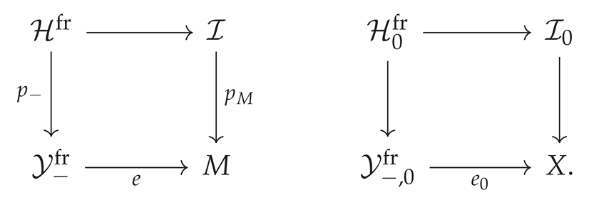
The varying invariant line remains a coordinate in the fiber product; it is not fixed to $\mathbb{C}{e}_1$.

Proposition A8

(Conifold-compatible Hecke incidence).  The map $p_{-}:{\mathcal{H}}^{\mathrm{fr}}\to {\mathcal{Y}}_{-}^{\mathrm{fr}}$ is projective. Over $B^{\circ }$, ${\mathcal{H}}^{\mathrm{fr}}$ is smooth, and ${\mathcal{H}}_0^{\mathrm{fr}}$ is the reduced normal-crossing union 

$${\mathcal{H}}_{\ker }\cup {\mathcal{H}}_{\mathrm{img}},{\mathcal{H}}_{\ker }\cap {\mathcal{H}}_{\mathrm{img}}={\mathcal{Y}}_{-}^{\mathrm{fr}}{\times }_{M}Z,$$

 where $Z=D_{\ker }\cap D_{\mathrm{img}}\simeq {\mathrm{Tot}}_{{\mathbb{P}}^1}\mathcal{O}(-2)$. The restrictions to both components are the smooth pullbacks of the kernel-line and image-line small resolutions of X. 

Proof. 

The projection $p_M$ is projective as a closed subscheme of $M\times {\mathbb{P}}^1$; projectivity is preserved under base change. The projection ${\mathcal{H}}^{\mathrm{fr}}\to \mathcal{I}$ is the base change of the smooth map  e , so its source is smooth because $\mathcal{I}$ is smooth. The corresponding map ${\mathcal{H}}_0^{\mathrm{fr}}\to {\mathcal{I}}_0$ is smooth. The latter incidence central fiber has local equation $\alpha \delta =0$ with $\alpha ,\delta$ independent regular parameters; the same remains true after smooth base change. Thus the two pullback divisors are smooth and meet transversely along the pullback of  Z . The Cartesian descriptions of the component projections follow from their fiber-product definitions. □

Let $I_X^H={\mathrm{IC}}_X^H$ and $R_X^H=i_{o*}{\mathbb{Q}}_o^H(-2)$. Fix the nonzero local corrected forward extension

$${ϵ}_X:R_X^H⟶I_X^H\left[1\right].$$

(A19)

Its normalization is the same nonzero generator used in Section 2.2 and Section 5.2.

Proposition A9

(Nonvanishing through smooth evaluation).  Assume $B^{\circ }\ne ⌀$, and let r be the relative complex dimension of $e_0$. The functor $e_0^{*}\left[r\right]$ is exact for the perverse t-structure, and it takes (A19) to a nonzero Yoneda extension on ${\mathcal{Y}}_{-,0}^{\mathrm{fr}}$: 

$${ϵ}_{\mathrm{ev}}:=e_0^{*}{ϵ}_X\left[r\right]:e_0^{*}{R}_X^H\left[r\right]⟶e_0^{*}{I}_X^H[r+1].$$

 Writing $T=e^{-1}\left(o\right)$ and $i_T:T\hookrightarrow {\mathcal{Y}}_{-,0}^{\mathrm{fr}}$, one has 

$$e_0^{*}{I}_X^H\left[r\right]\simeq {\mathrm{IC}}_{{\mathcal{Y}}_{-,0}^{\mathrm{fr}}}^H,e_0^{*}{R}_X^H\left[r\right]\simeq i_{T*}{\mathbb{Q}}_T^H\left[r\right](-2).$$

 The same class remains nonzero upon derived pullback to ${\mathcal{H}}_{\ker }$ along its map to ${\mathcal{Y}}_{-,0}^{\mathrm{fr}}$. 

Proof. 

Smooth pullback shifted by the relative dimension is exact on mixed-Hodge modules and commutes with intermediate extension; the first two identifications follow from smooth base change and the fact that  T  is smooth of dimension  r  over the node. Near a point of  T  the smooth morphism  e  has local analytic product coordinates, so the source conifold and its coefficient triangle pull back to the product of the conifold triangle with a smooth  r -dimensional factor. Extraordinary restriction to the transverse normal conifold slice recovers the local costalk attaching morphism

$${\mathbb{Q}}^H(-2)⟶H^1\left(i_o^{!}{I}_X^H\right)\simeq {\mathbb{Q}}^H(-2),$$

which is multiplication by the nonzero chosen source scalar. Therefore ${ϵ}_{\mathrm{ev}}$ cannot vanish. This argument uses the nonzero local costalk component, not a blanket claim that arbitrary smooth pullback is faithful on all derived Hom groups. On the kernel component the diagram is, locally in the smooth topology, the product of the original kernel-line resolution $m:D_{\ker }\to X$ with the same smooth factor. Its inverse image of the connecting morphism is the smooth pullback of $m^{*}{ϵ}_X$. Proposition 31 identifies the latter with a nonzero codimension-two Gysin map up to its nonzero scalar. Product pullback preserves this local Thom class, proving nonvanishing on the component and hence on the incidence correspondence prior to target pushforward. □

Proposition A10

(Node support with the invariant line unfrozen).  Retain the hypotheses and notation of Proposition A9. The inverse image of $T=e^{-1}\left(o\right)$ in the full invariant-line correspondence is 

$$T_{\mathcal{H}}:=p_{-}^{-1}\left(T\right)=T\times {\mathbb{P}}^1.$$

 Let $j_T:T_{\mathcal{H}}\hookrightarrow {\mathcal{H}}_0^{\mathrm{fr}}$ be the closed immersion. There is a canonical identification 

$$p_{-}^{*}\left(e_0^{*}{R}_X^H\left[r\right]\right)\simeq j_{T*}{\mathbb{Q}}_{T_{\mathcal{H}}}^H\left[r\right](-2).$$

 Since $\dim T_{\mathcal{H}}=r+1$, the only nonzero perverse cohomology object of this derived pullback is 

$${}^p{\mathcal{H}}^1\left(p_{-}^{*}{e}_0^{*}{R}_X^H\left[r\right]\right)\simeq j_{T*}{\mathbb{Q}}_{T_{\mathcal{H}}}^H[r+1](-2).$$

 In particular, the full exceptional ${\mathbb{P}}^1$ contributes to the correspondence source; it is absent from the fixed-line fiber used in the earlier adapted computation. 

Proof. 

For $A=0$ every line of  V  is invariant. Hence the Cartesian base change of the full incidence morphism over  T  is the trivial ${\mathbb{P}}^1$-bundle $T\times {\mathbb{P}}^1$, not a selected point in that fiber. Inverse-image base change for the closed immersion $i_T:T\hookrightarrow {\mathcal{Y}}_{-,0}^{\mathrm{fr}}$ gives

$$p_{-}^{*}{i}_{T*}{\mathbb{Q}}_T^H\left[r\right](-2)\simeq j_{T*}{\mathbb{Q}}_{T_{\mathcal{H}}}^H\left[r\right](-2).$$

The variety  T  is smooth of dimension  r , so its product with ${\mathbb{P}}^1$ is smooth of dimension $r+1$. Thus ${\mathbb{Q}}_{T_{\mathcal{H}}}^H[r+1]$ is perverse; the displayed pullback is its shift by $[-1]$. Closed pushforward is perverse  t -exact, giving the degree-one statement with no additional Tate twist. □

Appendix E.3. The Actual Modified-Higgs Morphism and Its Limitation

Proposition A11

(Elementary Hecke morphism over the determinant family).  There is an algebraic morphism of moduli functors 

$$q_{+}:{\mathcal{H}}^{\mathrm{fr}}⟶{\mathfrak{H}}_{2,d-1},$$

 where ${\mathfrak{H}}_{2,d-1}$ is the (unrestricted) stack of rank-two Higgs bundles of degree $d-1$. It sends $(E_{-},{\theta }_{-},\ell )$ to 

$$E_{+}:=\ker \left(E_{-}\to {\left(E_{-}\right)}_z/\ell \right),{\theta }_{+}:={\theta }_{-}{|}_{E_{+}}.$$

 The restriction is regular because ${\theta }_{-}\left(z\right)\ell \subset \ell$. Let $h_{-}:=\det \left(e\right)$ and let $h_{+}:{\mathfrak{H}}_{2,d-1}\to {\mathbb{A}}^1$ be determinant of the modified Higgs value at z, using the fixed trivialization of $K_C{|}_z$. Then 

$$h_{+}{q}_{+}=h_{-}{p}_{-},$$

 and the square 

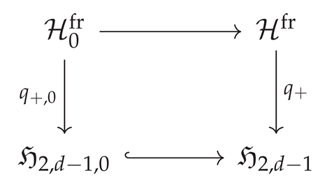 is Cartesian after the indicated restriction of the target to ${\mathfrak{H}}_{2,d-1,0}:=h_{+}^{-1}\left(0\right)$. In a source formal frame adapted to ℓ, one has 

$$A_{-}\left(w\right)=\left(\begin{array}{cc}a\left(w\right)& b\left(w\right)\\ c\left(w\right)& d\left(w\right)\end{array}\right),c\left(0\right)=0,A_{+}\left(w\right)=\left(\begin{array}{cc}a\left(w\right)& wb\left(w\right)\\ c\left(w\right)/w& d\left(w\right)\end{array}\right).$$

 The modified Higgs value depends on the first source jet, while its complete first jet depends on the second source jet. 

Proof. 

The elementary modification is the kernel of a universal surjection to a length-one sheaf supported at  z . Such a kernel commutes with base change in families for the flat universal length-one quotient. In an adapted formal frame its lattice is $\mathcal{O}{e}_1\oplus \mathcal{O}\left(w{e}_2\right)$. The displayed conjugation shows that preservation of this lattice is equivalent to $c\left(0\right)=0$; hence ${\theta }_{+}$ is regular and defines an algebraic family of Higgs fields on $E_{+}$. The construction is equivariant under changes of source frame by the explicit modified-frame transition in Proposition 10. Thus it defines a map into the unframed moduli stack without a canonical choice of modified framing. The characteristic polynomial is invariant under conjugation over $\mathbb{C}\left(\right(w\left)\right)$; regularity extends the equality of its coefficients across $w=0$. Therefore $\det A_{+}\left(0\right)=\det A_{-}\left(0\right)$ and the asserted fiber-product identity follows from equality of the defining functions. Finally $c\left(w\right)/w=c_1+c_{2}w+\dots$, proving the jet-order assertion. □

Lemma A5

(Modified Higgs value over the nodal evaluation locus).  On the λ-chart $\ell =\mathbb{C}(e_1+\lambda e_2)$, write $A_{-}\left(w\right)=A_0+w{A}_1+O\left(w^2\right)$, with $A_1=\left(\begin{array}{cc}{a}_1& b_1\\ c_1& d_1\end{array}\right)$. Over $A_0=0$ the modified value in the adapted modified lattice is 

$$A_{+}\left(0\right)=\left(\begin{array}{cc}0& 0\\ {\gamma }_1\left(\lambda \right)& 0\end{array}\right),{\gamma }_1\left(\lambda \right)=c_1+(d_1-a_1)\lambda -b_1{\lambda }^2.$$

 Consequently the image of the node-supported coefficient under the geometric target map lies in the nilpotent-evaluation locus. For ${\gamma }_1\left(\lambda \right)\ne 0$ the modified Higgs value is regular nilpotent; for ${\gamma }_1\left(\lambda \right)=0$ it is zero. The zero scheme of ${\gamma }_1$ varies with the full invariant line and cannot be recovered from the frozen-line chart alone. 

Proof. 

Change source frame by $B_{\lambda }=\left(\begin{array}{cc}1& 0\\ \lambda & 1\end{array}\right)$. As in Section 3.1, its lower-left matrix entry is $\gamma \left(w\right)=c\left(w\right)+(d\left(w\right)-a\left(w\right))\lambda -b\left(w\right){\lambda }^2$. When $A_0=0$ the entire adapted leading matrix vanishes, and $\gamma \left(w\right)=w{\gamma }_1\left(\lambda \right)+O\left(w^2\right)$. Conjugation by $\mathrm{diag}(1,w)$ gives the displayed modified value. Its trace, determinant, and rank are immediate. The polynomial ${\gamma }_1$ is the chart expression of the invariant-line quadratic for $A_1$; its zero locus transforms covariantly on the second chart. □

Remark A9

(What the target map does and does not calculate).  The morphism $q_{+}$ is an actual geometric Hecke target map. It is not the vector-bundle projection $\tilde{X}\to {\mathbb{P}}^1$ of Section 5. The framed correspondence includes choices of source framing; its projection to the unframed target must not be declared proper on the basis of properness of $p_{-}$. For a derived target calculation one must specify the appropriate stack or finite-type chart, the correspondence coefficient, and whether $R{q}_{+*}$ or $R{q}_{+!}$ is being applied. The preceding propositions establish the pre-target arrow, not its direct image. The separate kernel-branch inverse and Gysin argument of Theorem 8 proves nonvanishing on U, and Theorem 9 identifies its degree-two class on $U^{\prime }$. Neither conclusion follows from the evaluation diagram alone. 

Appendix E.4. The Nilpotent Transverse Slice in Two-Step Convolution

Put $\mathcal{O}=\mathbb{C}\left[\right[w\left]\right]$, $\mathcal{K}=\mathbb{C}\left(\right(w\left)\right)$, $V={\mathbb{C}}^2$, and ${\mathsf{\Lambda }}_0=\mathcal{O}\otimes V$. Let $\mathcal{S}$ be the bounded affine-Grassmannian Schubert closure of coweight $(2,0)$, and let $\mathcal{C}={\mathrm{Gr}}^{\le (1,0)}\tilde{\times }{\mathrm{Gr}}^{\le (1,0)}$ be the convolution space of upper elementary modifications, with proper terminal map $m_{21}:\mathcal{C}\to \mathcal{S}$. Let ${\mathsf{\Lambda }}_{*}:=w^{-1}{\mathsf{\Lambda }}_0$ be the $(1,1)$ point.

Proposition A12

(Explicit nilpotent lattice slice).  For $A\in \mathcal{N}:=\{A\in {\mathfrak{sl}}_2:\det A=0\}$ define 

$${\mathsf{\Lambda }}_A:=\left(1+w^{-1}A\right){\mathsf{\Lambda }}_{*}.$$

 This is a lattice satisfying ${\mathsf{\Lambda }}_0\subset {\mathsf{\Lambda }}_A\subset w^{-2}{\mathsf{\Lambda }}_0$ and ${\dim }_{\mathbb{C}}({\mathsf{\Lambda }}_A/{\mathsf{\Lambda }}_0)=2$. There is a canonical $\mathbb{C}$-linear identification 

$${\tau }_A:V\stackrel{\sim }{\to }{\mathsf{\Lambda }}_A/{\mathsf{\Lambda }}_0,v⟼w^{-1}v+w^{-2}Av\left(\mathrm{mod}{\mathsf{\Lambda }}_0\right),$$

 under which multiplication by w is exactly A. The map $A\mapsto {\mathsf{\Lambda }}_A$ identifies $\mathcal{N}$ with the reduced transverse slice in the affine Grassmannian at ${\mathsf{\Lambda }}_{*}$. The scheme structure and inverse are supplied by the type-A slice isomorphism [10]. 

Proof. 

For a trace-zero two-by-two matrix with determinant zero, Cayley–Hamilton gives $A^2=0$. Therefore ${(1+w^{-1}A)}^{-1}=1-w^{-1}A$, and $\det (1+w^{-1}A)=1$. To verify ${\mathsf{\Lambda }}_0\subset {\mathsf{\Lambda }}_A$, take $x\in {\mathsf{\Lambda }}_0$. Then $(1-w^{-1}A)x\in w^{-1}{\mathsf{\Lambda }}_0={\mathsf{\Lambda }}_{*}$, so $x\in {\mathsf{\Lambda }}_A$. The upper inclusion is immediate from $A{\mathsf{\Lambda }}_0\subset {\mathsf{\Lambda }}_0$. The lattice has determinant valuation $-2$, giving the indicated quotient dimension. Every class modulo ${\mathsf{\Lambda }}_0$ has a representative of the form $w^{-1}v+w^{-2}Av$ for a constant vector $v\in V$; independence follows because a representative in ${\mathsf{\Lambda }}_0$ forces first $Av=0$ and then $v=0$. Moreover

$$w{\tau }_A\left(v\right)=v+w^{-1}Av\equiv w^{-1}Av+w^{-2}{A}^{2}v={\tau }_A\left(Av\right)\left(\mathrm{mod}{\mathsf{\Lambda }}_0\right).$$

This proves the asserted intertwining relation. The inverse graph description recovers  A  from the action of  w  on ${\mathsf{\Lambda }}_A/{\mathsf{\Lambda }}_0$; the reduced scheme-level identification of this graph chart with the transverse slice is the established type- A  nilpotent/loop-Grassmannian comparison cited in the statement. The calculation above verifies its formula in rank two. □

Proposition A13

(Cartesian Springer–convolution restriction).  The pullback of the two-step convolution map to the nilpotent slice of Proposition A12 identifies with 

$$\sigma :Z⟶\mathcal{N},Z=\{(A,\ell ):\mathrm{im}A\subset \ell \subset \ker A\}\simeq {\mathrm{Tot}}_{{\mathbb{P}}^1}\mathcal{O}(-2).$$

 Explicitly, an intermediate lattice ${\mathsf{\Lambda }}_0\subset {\mathsf{\Lambda }}_1\subset {\mathsf{\Lambda }}_A$ corresponds under ${\tau }_A$ to the one-dimensional subspace $\ell ={\tau }_A^{-1}({\mathsf{\Lambda }}_1/{\mathsf{\Lambda }}_0)\subset V$. The correspondence defines the Cartesian square 

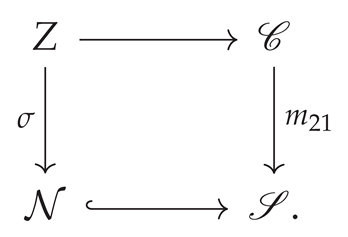
 The square is taken with the reduced transverse-slice structure of Proposition A12. 

Proof. 

The intermediate lattice ${\mathsf{\Lambda }}_1$ is an $\mathcal{O}$-submodule of ${\mathsf{\Lambda }}_A$ containing ${\mathsf{\Lambda }}_0$, with a one-dimensional $\mathbb{C}$ quotient ${\mathsf{\Lambda }}_1/{\mathsf{\Lambda }}_0$. Under ${\tau }_A$, ${\mathsf{\Lambda }}_1/{\mathsf{\Lambda }}_0$ is a line $\ell \subset V$. It is $\mathcal{O}$-stable exactly when $A\ell \subset \ell$, since multiplication by  w  acts as  A . Because  A  is nilpotent and  ℓ  is one-dimensional, ${A|}_{\ell }=0$; hence $\ell \subset \ker A$. The induced action on $V/\ell$ is again nilpotent on a one-dimensional space and therefore zero. Thus $\mathrm{im}A\subset \ell$. Conversely these two containments imply $A\ell \subset \ell$, and the inverse image of ${\tau }_A(\ell )$ is the requisite intermediate lattice. The two constructions commute with change of base and are inverse on the corresponding relative flag functors; together with the scheme-level transverse-slice identification of the preceding proposition, they establish the Cartesian comparison. For fixed  ℓ  the space of matrices with $\mathrm{im}A\subset \ell \subset \ker A$ is $\mathrm{Hom}(V/\ell ,\ell )$. On $\mathbb{P}\left(V\right)$ this is $\mathcal{O}(-2)$, proving the total-space identification. For $A\ne 0$ the line is unique; at $A=0$ the fiber is ${\mathbb{P}}^1$. □

Corollary A1

(The Springer Tate channel is a convolution summand).  The restriction of the pure convolution direct image to the nilpotent slice has the decomposition 

$$R{\sigma }_{*}{\mathbb{Q}}_Z^H\left[2\right]\simeq {\mathrm{IC}}_{\mathcal{N}}^H\oplus i_{o*}{\mathbb{Q}}_o^H(-1).$$

 The point-supported ${\mathbb{Q}}^H(-1)$ summand is the local geometric-Satake contribution associated with the $(1,1)$ (determinant-representation) stratum in $V_{(1,0)}\otimes V_{(1,0)}\simeq V_{(2,0)}\oplus V_{(1,1)}$. It is not an identification of this pure Tate summand with the source forward-extension quotient ${\mathbb{Q}}^H(-2)$ or with an associated source extension morphism. 

Proof. 

The proper map $\sigma$ is semismall: its unique positive-dimensional fiber is ${\mathbb{P}}^1$ over the codimension-two point  o . The pure decomposition theorem gives the intersection complex of the open stratum and a point-supported contribution. Proper base change and $H^2({\mathbb{P}}^1,\mathbb{Q})=\mathbb{Q}(-1)$ fix its multiplicity and twist. By the Cartesian slice identification, this is the restriction of the two-step convolution decomposition. Geometric Satake identifies the two relevant IC supports with the weights $(2,0)$ and $(1,1)$ in the tensor square of the standard representation [9,21]. The source conifold quotient has a different Tate type, so the final nonidentification follows from its normalization. □

Lemma A6

(The global minuscule convolution surface).  The two-step minuscule convolution surface is 

$$\mathcal{C}\simeq {\mathbb{P}}_{{\mathbb{P}}^1}\left(\mathcal{O}\left(1\right)\oplus \mathcal{O}(-1)\right)\simeq {\mathbb{F}}_2.$$

 The Springer slice Z is the complement of an appropriate section of this projective surface, so Z is not the entire convolution space. 

Proof. 

An elementary upper lattice ${\mathsf{\Lambda }}_1$ is determined by a line $\ell \subset V={\mathsf{\Lambda }}_0/w{\mathsf{\Lambda }}_0$ and has the form ${\mathsf{\Lambda }}_1={\mathsf{\Lambda }}_0+w^{-1}\ell$. The possible next elementary lattices are the lines in the rank-two bundle ${\mathsf{\Lambda }}_1/w{\mathsf{\Lambda }}_1$ on $\mathbb{P}\left(V\right)$. The inclusions $w{\mathsf{\Lambda }}_1\subset {\mathsf{\Lambda }}_0\subset {\mathsf{\Lambda }}_1$ give an exact sequence of bundles

$$0⟶{\mathsf{\Lambda }}_0/w{\mathsf{\Lambda }}_1\simeq V/\ell \simeq \mathcal{O}\left(1\right)⟶{\mathsf{\Lambda }}_1/w{\mathsf{\Lambda }}_1⟶{\mathsf{\Lambda }}_1/{\mathsf{\Lambda }}_0\simeq \ell \simeq \mathcal{O}(-1)⟶0.$$

Its extension class lies in ${\mathrm{Ext}}_{{\mathbb{P}}^1}^1(\mathcal{O}(-1),\mathcal{O}\left(1\right))\simeq H^1({\mathbb{P}}^1,\mathcal{O}\left(2\right))=0$. The rank-two bundle therefore splits as $\mathcal{O}\left(1\right)\oplus \mathcal{O}(-1)$. Its projective-line bundle is the Hirzebruch surface ${\mathbb{F}}_2$. After twisting by $\mathcal{O}(-1)$ the bundle is $\mathcal{O}\oplus \mathcal{O}(-2)$; removing the infinity section of its projectivization gives the total space of $\mathcal{O}(-2)$. The Cartesian slice of Proposition A13 selects precisely this open resolution over the nilpotent slice. □

Appendix E.5. Closed Calculations and Remaining Target-Morphism Problem

Proposition A14

(Precisely delimited geometric completion).  On a nonempty evaluation-regular locus the following constructions are defined by algebraic maps and have the indicated properties: 

(i)

 Smooth evaluation produces the Cartesian determinantal and invariant-line incidence diagrams and the normal-crossing central correspondence (Proposition A8). 

(ii)

 The universal local forward extension remains nonzero after normalized evaluation pullback and after pullback to the kernel incidence component (Proposition A9). 

(iii)

 Elementary modification gives an actual map to the unframed modified-Higgs stack, preserving the determinant family (Proposition A11). 

(iv)

 The Springer overlap is a Cartesian nilpotent slice of bounded $G{L}_2$ convolution and its $\mathbb{Q}(-1)$ channel is the determinant Satake summand (Proposition A13 and Corollary A1). 

 The value of 

$$R{q}_{+\sigma }\left(p_{-}^{*}{ϵ}_{\mathrm{ev}}\otimes {\mathcal{K}}_H\right),\sigma \in \{*,!\},$$

 on the chosen unframed mixed-Hodge-module category is not calculated by (i)–(iv) alone . The later kernel-branch argument of Theorem 8 proves nonvanishing on U, and the finite-open theorem 9 identifies the degree-two class on $U^{\prime }$. A canonical realization of an unrelated proper nodal threefold, and arbitrary-kernel target calculations, are still absent. 

Proof. 

The first four conclusions are the cited geometric and Hodge-module calculations. The last assertion concerns what follows from the  four listed constructions alone . The actual target results of Theorems 8 and 9 use additional inverse-branch, finite-correspondence, and equivariant comparisons. A computation on the auxiliary kernel-line projection does not replace those maps, and an unrelated nodal threefold still requires independent source-realization data. □

References

- Beilinson, A.A.; Bernstein, J.; Deligne, P. Faisceaux pervers; Société Mathématique de France: Astérisque, 1982; Vol. 100, pp. 5–171. [Google Scholar]
- Saito, M. Modules de Hodge polarisables. Publ. Res. Inst. Math. Sci. 1988, 24, 849–995. [Google Scholar] [CrossRef]
- Saito, M. Mixed Hodge Modules. Publ. Res. Inst. Math. Sci. 1990, 26, 221–333. [Google Scholar] [CrossRef]
- MacPherson, R.; Vilonen, K. Elementary Construction of Perverse Sheaves. Invent. Math. 1986, 84, 403–435. [Google Scholar] [CrossRef]
- Beilinson, A.A. How to Glue Perverse Sheaves. In K-Theory, Arithmetic and Geometry (Moscow, 1984–1986); Lecture Notes in Mathematics; Springer: Berlin, 1987; Vol. 1289, pp. 42–51. [Google Scholar]
- Rahman, A. Perverse Extensions and Limiting Mixed Hodge Structures for Conifold Degenerations, 2026. arXiv arXiv:math.
- Rahman, A. Mixed Hodge Modules and Canonical Perverse Extensions for Multi-Node Conifold Degenerations. arXiv 2026, arXiv:math. [Google Scholar]
- Slodowy, P. Simple Singularities and Simple Algebraic Groups. In Lecture Notes in Mathematics; Springer, 1980; Vol. 815. [Google Scholar] [CrossRef]
- Mirković, I.; Vilonen, K. Geometric Langlands Duality and Representations of Algebraic Groups over Commutative Rings. Ann. Math. 2007, 166, 95–143. [Google Scholar] [CrossRef]
- Mirković, I.; Vybornov, M.; Krylov, V. Comparison of Quiver Varieties, Loop Grassmannians and Nilpotent Cones in Type A. Adv. Math. 2022, 407, 108397. [Google Scholar] [CrossRef]
- Rahman, A. Hodge Atoms at Conifold Degenerations: F -Bundles, Limiting Mixed Hodge Modules, and the Rigid–Flexible Decomposition, 2026. arXiv arXiv:math.
- Kapustin, A.; Witten, E. Electric–Magnetic Duality and the Geometric Langlands Program. Commun. Number Theory Phys. 2007, 1, 1–236. [Google Scholar] [CrossRef]
- Narasimhan, M.S.; Ramanan, S. Geometry of Hecke cycles. I; Ramanujam—A Tribute, C. P., Ed.; Springer; Tata Institute of Fundamental Research Studies in Mathematics, 1978; Vol. 8, pp. 291–345. [Google Scholar]
- Hwang, J.M. Tangent vectors to Hecke curves on the moduli space of rank 2 bundles over an algebraic curve. Duke Math. J. 2000, 101, 179–187. [Google Scholar] [CrossRef]
- Hwang, J.M.; Ramanan, S. Hecke curves and Hitchin discriminant. Ann. Sci. De l’École Norm. Supérieure 2004, 37, 801–817. [Google Scholar] [CrossRef]
- Sun, X. Minimal rational curves on moduli spaces of stable bundles. Math. Ann. 2005, 331, 925–937. [Google Scholar] [CrossRef]
- Milnor, J. Singular Points of Complex Hypersurfaces. In Annals of Mathematics Studies; Princeton University Press: Princeton, 1968; Vol. 61. [Google Scholar]
- Schmid, W. Variation of Hodge Structure: The Singularities of the Period Mapping. Invent. Math. 1973, 22, 211–319. [Google Scholar] [CrossRef]
- Lusztig, G. Green Polynomials and Singularities of Unipotent Classes. Adv. Math. 1981, 42, 169–178. [Google Scholar] [CrossRef]
- Mirković, I.; Vybornov, M. On Quiver Varieties and Affine Grassmannians of Type A . Comptes Rendus Mathématique 2003, 336, 207–212. [Google Scholar] [CrossRef]
- Fedorov, R. Satake Equivalence for Hodge Modules on Affine Grassmannians. arXiv 2021, arXiv:math. [Google Scholar]
- Richarz, T.; Scholbach, J. The Motivic Satake Equivalence. Math. Ann. 2021, 380, 1595–1653. [Google Scholar] [CrossRef]
- Cautis, S.; Dodd, C.; Kamnitzer, J. Associated Graded of Hodge Modules and Categorical sl 2 Actions. Sel. Math. (New Series) 2021, 27(22), 1603.07402. [Google Scholar] [CrossRef]
- Gaitsgory, D. Construction of Central Elements in the Affine Hecke Algebra via Nearby Cycles. Invent. Math. 2001, 144, 253–280. [Google Scholar] [CrossRef]
- Achar, P.N.; Riche, S. Higher Nearby Cycles and Central Sheaves on Affine Flag Varieties. J. Singul. 2024, 27, 1–30, [2305.11696. [Google Scholar] [CrossRef]
- Achar, P.N.; Riche, S. Central Sheaves on Affine Flag Varieties. In Panoramas et Synthèses; Société Mathématique de France, 2025; Vol. 64. [Google Scholar]
- Salmon, A. Unipotent Nearby Cycles and Nearby Cycles over General Bases. J. Singul. 2024, 27, 31–46, [2401.16746. [Google Scholar] [CrossRef]
- Elias, B. Gaitsgory’s Central Sheaves via the Diagrammatic Hecke Category. In Memoirs of the American Mathematical Society; American Mathematical Society, 2026; Vol. 319, p. 1811.06188. [Google Scholar] [CrossRef]
- Donagi, R.; Pantev, T.; Simpson, C. Twistor Hecke Eigensheaves in Genus 2, 2024. arXiv arXiv:math.
- Witten, E. More on Gauge Theory and Geometric Langlands. Adv. Math. 2018, arXiv:hep327, 624–707. [Google Scholar] [CrossRef]
- He, S.; Walpuski, T. Hecke Modifications of Higgs Bundles and the Extended Bogomolny Equation. J. Geom. Phys. 2019, 146, 103487. [Google Scholar] [CrossRef]
- Tubach, S. Mixed Hodge Modules on Stacks. Forum Math. Sigma 2025, 13, e175, [2407.02256. [Google Scholar] [CrossRef]
- Beauville, A. Orthogonal Bundles on Curves and Theta Functions. Ann. De l’Institut Fourier 2006, 56, 1405–1418. [Google Scholar] [CrossRef]
- Gaitsgory, D.; Raskin, S. Proof of the Geometric Langlands Conjecture I: Construction of the Functor, 2025. arXiv, Version 3; 2025, arXiv:math. [Google Scholar]
- Davison, B.; Hennecart, L.; Kinjo, T.; Schiffmann, O.; Vasserot, E. Hecke Operators on Symplectic Surfaces and χ -Independence, 2026. arXiv arXiv:math.
- Rahman, A. Recollement Defects and MacPherson–Vilonen Boundary Residuals, 2026. Preprints.org 2026, version 1. [Google Scholar] [CrossRef]
- Rahman, A. Bivariant Hodge Atoms I: Hecke Collisions and Mixed-Hodge Coefficient Extensions, 2026. Preprints.org preprint, version 1. posted. 2026. [Google Scholar] [PubMed]
- González, M. Very Stable Regular G -Higgs Bundles. arXiv 2025, arXiv:math. [Google Scholar]
- Dimca, A. Sheaves in Topology. In Universitext; Springer, 2004. [Google Scholar] [CrossRef]
Disclaimer/Publisher’s Note: The statements, opinions and data contained in all publications are solely those of the individual author(s) and contributor(s) and not of MDPI and/or the editor(s). MDPI and/or the editor(s) disclaim responsibility for any injury to people or property resulting from any ideas, methods, instructions or products referred to in the content. |
© 2026 by the authors. Licensee MDPI, Basel, Switzerland. This article is an open access article distributed under the terms and conditions of the Creative Commons Attribution (CC BY) license (http://creativecommons.org/licenses/by/4.0/).
Copyright: This open access article is published under a Creative Commons CC BY 4.0 license, which permit the free download, distribution, and reuse, provided that the author and preprint are cited in any reuse.