

Submitted:
20 October 2026
Posted:
21 October 2026
You are already at the latest version
Abstract
Missing-data strategies are often compared using a single cohort or prediction model, making it difficult to distinguish imputation-specific effects from benefits due to the downstream learner or prediction averaging. We conducted a leakage-controlled factorial simulation in two public cardiac cohorts (n = 299 and n = 918), comparing six strategies across three missingness mechanisms, three missingness rates (10–50%), ten seeds, and three learners. A four-arm analysis further examined the contribution of multiple imputation relative to single imputation and model averaging. Strategy effects depended on the learner: exploratory strategy-by-learner interactions were significant in both cohorts, while no strategy effect survived Holm correction for penalised logistic regression. Prediction-layer-pooled multiple imputation ranked first for the tree-based learners in the larger cohort. In the smaller cohort with XGBoost, its paired median AUROC difference versus a bagged mean-imputation ensemble was −0.003 (Holm-adjusted p = 0.275); because equivalence was not tested, this result does not establish that the strategies perform equivalently. No consistent strategy-by-missingness-mechanism interaction was found. These findings support evaluating missing-data handling jointly with the prediction model and interpreting apparent strategy advantages in light of ensemble effects. This research offers new insights into strategies for handling missing data.
Keywords:
missing data
; multiple imputation
; clinical prediction
; machine learning
; cardiac prediction
; model evaluation
; factorial simulation
1. Introduction
Heart failure (HF) affects an estimated 64 million people worldwide [1] and carries a five-year mortality approaching 50%, with readmission and death clustering in the early post-discharge "vulnerable phase" [2]. Risk-prediction models (increasingly machine-learning (ML) models built on routinely collected electronic health record (EHR) variables) are increasingly used for triage, outpatient follow-up planning, and quality benchmarking in HF programmes. A recent systematic review and meta-analysis of 346 ML models for HF mortality and readmission reported pooled discrimination of approximately 0.70–0.81 in the area under the receiver operating characteristic curve (AUROC), but simultaneously found that 82.9% of studies were at high risk of bias, most commonly because of inadequate validation, absent replication, and (critically for the present study) predictors unavailable at the moment of prediction and optimistic handling of incomplete data [3]. The same review identified another reporting deficit: discrimination is reported almost universally, whereas calibration (the correspondence between predicted and observed probabilities on which any threshold-based clinical decision depends) is reported only rarely [4,5,6,7].
A structural weakness of EHR-based cardiac models is that laboratory and functional covariates are frequently missing: in routine HF cohorts, 10–50% of entries for creatinine, sodium, ejection fraction and comparable variables are typically absent [8], and the probability of being missing is itself systematically associated with patient age, severity, and care setting rather than being purely random [9]. A large methodological toolbox exists for this problem, from simple mean or median substitution, through k-nearest-neighbour (kNN) [10] and multiple imputation by chained equations (MICE), to iterative random-forest imputation (MissForest) [11] and the native sparsity-aware handling built into modern gradient-boosted learners [12,13], and comparative studies in cardiac populations regularly crown a "winner": MICE in XGBoost readmission pipelines and in heart failure with preserved ejection fraction (HFpEF) mortality prediction, kNN in intensive-care HF cohorts, MissForest elsewhere [14,15,16]. These recommendations, however, rest almost entirely on single-cohort evaluations run under a single realised missingness pattern with a single random seed and a single downstream learner, without controlled variation of the missingness mechanism (missing completely at random (MCAR), missing at random (MAR) and missing not at random (MNAR)) [17,18] or of the missingness rate, without formal statistical testing of between-strategy differences, without calibration, and without asking whether the winning strategy retains its rank in any other cohort or under any other learner. A related body of work has examined prediction-layer pooling of multiple imputations [19,20,21], but these studies have not simultaneously controlled for the generic ensemble-variance-reduction effect, the missingness mechanism, and the learner type, leaving the MICE-specific increment unidentified.
Studies in other clinical domains report similarly mixed results. In dementia classification, MICE yielded the highest accuracy for random forest and logistic regression, whereas the support vector machine performed best with median imputation [22], a learner-dependent ranking reported descriptively but not tested as an interaction. In diabetes and mixed healthcare datasets, MissForest outperformed MICE and kNN in most evaluation metrics [23,24], a "winner" different from the cardiac-population recommendations above. In deep-learning lung-cancer survival models, the ranking of mean, kNN, MICE and MissForest changed with both the dataset and the model, leading the authors to sidestep imputation entirely through masked attention [25,26]. Together, these findings are consistent with learner- and domain-dependence, yet none of these studies crossed missingness mechanisms (where specified, missingness was MCAR only), none separated the imputation effect from the generic ensemble effect, and none asked whether strategy rankings transfer across cohorts. Another question (whether imputation choice differentially affects model performance across patient subgroups) has been raised in HF readmission prediction, where the imputation method changed gender-based performance disparity [27], and remains unaddressed in all of the studies above. A 2026 simulation study in a single real-world cardiac cohort of 8,245 patients compared complete-case analysis, two MICE variants, MissForest and kNN under 18 MAR scenarios and reported that kNN was the most stable and fastest method while MICE degraded under non-linear or extreme missingness, but it varied only the missingness proportion, used a single cohort and a single regression learner, and did not separate imputation-specific from generic ensemble effects [28]. The literature contains multiple mutually inconsistent recommendations, each plausibly reporting a local optimum, but whether the disagreement reflects true cohort effects, seed noise, or learner sensitivity has, to our knowledge, never been formally tested in cardiac prediction (PubMed/Scopus search, 2026-08-19: "(imputation) AND (missing data) AND (heart failure OR cardiac) AND (MCAR OR MAR OR MNAR)"; no study formally testing strategy × mechanism interaction across multiple learners was identified).
We designed a leakage-controlled, dual-cohort, multi-learner full-factorial simulation study framed as an applied methodological comparison rather than a new imputation method. Because missing-data handling is outcome-agnostic, we deliberately spanned two cardiac outcomes (death during follow-up in HF (UCI) and structural heart disease (Kaggle)) to test whether imputation effects generalise across cardiac prediction tasks rather than within HF alone. Six widely used strategies (mean; median; kNN; MICE with m = 5, pooled at the prediction layer; MissForest; XGBoost-native handling) were evaluated under 3 missingness mechanisms × 3 missingness rates in two publicly available cohorts of deliberately contrasting size and case mix (UCI, n = 299; Kaggle, n = 918), each condition replicated with 10 random seeds, and each imputed dataset fed to three downstream learners (XGBoost, logistic regression, random forest) with identical train-test splits and missingness masks. Beyond discrimination, we assessed calibration (Brier score, calibration intercept and slope), the strategy × mechanism interaction by three-way ANOVA, the transferability of strategy rankings between cohorts by Spearman rank correlation, and, using SHapley Additive exPlanations (SHAP), the stability of feature-importance explanations against the complete-data reference. The analysis was framed around two falsifiable null hypotheses: H0-1, that imputation strategy does not interact with the downstream learner, tested at two levels, an omnibus repeated-measures interaction term and a targeted contrast on the key S4-versus-simple effect; and H0-2, that imputation strategy does not interact with the missingness mechanism. Rejection of H0-2 (not the selection of another single-learner best strategy) would be required before any mechanism-tailored strategy recommendation could be justified. The learner-dependent direction of the strategy effect reported in Section 3 (present for tree-based learners, absent for the penalised logistic regression tested) is an observed finding of this design, not an a priori prediction.
2. Materials and Methods
2.1. Study Design and Data Sources
This was a full-factorial simulation study embedded in two retrospective, publicly available, de-identified cohorts; no new human-subject data were collected, and both source datasets are distributed under open licences, so ethical approval was not required.
UCI cohort. The Heart Failure Clinical Records dataset [29,30] contains 299 patients with HF enrolled at Firoozgar Hospital (Tehran, Iran; enrolment 2015), with all-cause death during the follow-up period (median 130 days) as the outcome (96 events, 32.1%) and 12 recorded variables. The follow-up-duration variable (time) was excluded a priori (Section 2.2), leaving 11 candidate predictors: age, anaemia, creatinine phosphokinase, diabetes, ejection fraction, high blood pressure, platelets, serum creatinine, serum sodium, sex, and smoking. With 72 events in the 75% training partition and 11 predictors, the events-per-variable ratio was ≈ 6.5 (below the classic EPV ≥ 10 heuristic [31,32]) which contextualises the small-cohort calibration findings in Section 3.5.
Kaggle cohort. The Heart Failure Prediction dataset [33] aggregates five heart-disease sources (Cleveland, Hungary, Switzerland, Long Beach VA, and the Statlog set; original collection 1988–2015) into 918 patients, with structural heart disease as the outcome (508 events, 55.3%) and 11 predictors after integer encoding of five categorical variables (sex, chest-pain type, resting ECG, exercise angina, ST slope). These five variables carry a nominal label encoding in the released file (sex; four clinical categories each); the encoded integer frame is passed unchanged to every learner, so the penalised logistic regression receives ordinal integers rather than a one-hot design and imposes an ordering and equal spacing that the underlying categories do not have (Section 4.5). Because the Statlog source partially overlaps the Cleveland source, we verified that the released file contains no exact duplicate rows (0/918).
The two cohorts were chosen to be maximally heterogeneous in sample size (3-fold), event fraction (1.7-fold), and baseline discriminative performance (0.22 AUROC range across three learners; Table 3), so that any finding reproduced in both could be argued robust, and any finding confined to one could be identified as cohort-specific. Test folds comprised approximately 75 patients (≈ 24 events) in UCI and approximately 230 patients (≈ 127 events) in Kaggle. The two cohorts also differ sharply in demographic composition (Table 3): mean age 60.8 ± 11.9 years with 35.1% female patients (105/299) in UCI, versus 53.5 ± 9.4 years with 21.0% female patients (193/918) in Kaggle.
2.2. Leakage Control
Two leakage channels were closed before any modelling. First, follow-up duration was excluded from the UCI predictor set: the outcome (death within follow-up) is defined on the follow-up interval, so a model using follow-up length as a covariate is logically circular and capitalises on immortal-time-type information [34]; in a leakage-inclusive sensitivity analysis of the same data (10 seeds, complete-data baseline), this single variable inflated mean AUROC from 0.713 ± 0.041 to 0.910 ± 0.030 (a difference of +0.197; Section 3.1, Table S6). Second, imputer leakage was eliminated by fitting every imputation model on the training partition only and applying the fitted imputer to the held-out test partition; no test-fold information entered imputation-parameter estimation, and in the rewritten simulation the missingness-mechanism parameters themselves (age median, P75 thresholds) are likewise training-partition-defined (Section 2.3). Two scenario-level parameters are computed on the full cohort by construction and are disclosed rather than eliminated: the MNAR marginal-rate calibration weights (a property of the simulation generator, shared identically across strategies) and the principal component analysis (PCA) severity factor of the correlated-missingness arm (Section 2.3). No other variable in either cohort encodes the outcome or post-outcome information.
2.3. Missingness Simulation
Missingness was induced only in the continuous covariates, six continuous variables in UCI (age and five laboratory variables: creatinine phosphokinase, ejection fraction, platelets, serum creatinine, serum sodium) and five clinical variables in Kaggle (age, resting blood pressure, cholesterol, maximum heart rate, ST depression), because these mirror the variables most often incomplete in EHR-based cardiac research. Three mechanisms were implemented for each variable v by assigning each patient a missingness probability p and drawing a Bernoulli mask:
MCAR: p = r for all patients, where r ∈ {0.1, 0.3, 0.5};
MAR: missingness depended on a fully observed variable other than v itself (patient age above the training-partition median): p = 1.8 r′ for older and 0.2 r′ for younger patients (clipped at 0.95), with r′ = r × 6/5 (UCI) or r × 5/4 (Kaggle) so that the overall marginal rate equals the nominal r after compensating for the unmasked driver. The driver variable (age) was never masked in this arm, so the missingness probability of every masked variable depends only on values that remain observed in the analysed data, the MAR label is exact for all masked variables, resolving the driver-masking contamination disclosed in earlier versions of this design;
MNAR: missingness depended on the would-be value of v itself (upper quartile, > P75, with P75 defined on the training partition). Weights were calibrated so that the marginal missingness rate equals the nominal rate r: p = p_high = 2.706 r (clipped at 0.95) for high-quartile values and p = p_low = (r − 0.25 × p_high) / 0.75 for low-quartile values.
Mask generation relative to splitting. For the MAR and MNAR arms, masks were generated after the stratified train-test split, with every mechanism parameter (the age median, the per-variable P75 thresholds) estimated on the training partition only and then applied to both partitions; the simulation generator therefore uses no test-fold information, matching the deployment setting in which mechanism parameters would be properties of the training population. MCAR masks involve no estimated parameters and are identical to the initial release. Consequently, all MAR/MNAR results in this report derive from the rewritten simulation (marginal rates verified, Table S11); MCAR results are unchanged.
Correlated-missingness sensitivity arm. The main mechanisms generate masks independently across variables; real EHR missingness is correlated (tests are ordered in panels) and jointly severity-dependent. To probe robustness to this structural assumption, a latent severity factor z (the first principal component of the standardised continuous predictors) drove the missingness probability of every continuous variable simultaneously through a logistic link, p = σ (a + γz) with γ = 1.0, capped at 0.95, with the intercept a solved by bisection so that the marginal rate equals the nominal rate r exactly (observed 0.100/0.301/0.500 in both cohorts). This construction makes missingness both correlated across variables and value-dependent. The PCA loadings and the intercept calibration are parameters of the simulation generator computed on the full cohort before splitting, they define the missingness scenario applied identically to all strategies and are not part of any fitted imputation or prediction pipeline; the deployment-consistent masking protocol of the main design (training-partition-defined parameters, Section 2.3) is therefore not required for interpretation of this arm. The arm was run for L1 and L3 only; L2 was omitted because its null strategy effect (Section 3.2) leaves no ranking structure to preserve. Results are reported in Section 3.10 (Figure 8).
Seed architecture. Two seed layers were used by design: a design seed (0–9) drove the missingness mask and the stratified train-test split, while learner random states and the five internal MICE draws (imputation seeds 0–4) were held fixed across design seeds. Consequently, for deterministic imputers (S1, S2) the only seed-to-seed variation is the split and mask; seed-level standard deviations therefore include split noise and are conservative, while strategy comparisons are protected by seed-level blocking in the Friedman tests (Section 2.7).
Mechanism and rate were fully crossed (3 × 3 = 9 conditions per cohort). For each condition, the full feature matrix was partitioned 75%/25% into training and test sets by stratified sampling on the outcome (scikit-learn train_test_split, test_size = 0.25), and the missingness mask was then applied (with mechanism parameters estimated on the training partition (Section 2.3)) so that all strategies within a given condition-seed faced identical train/test splits, masks, and downstream randomness, isolating the imputation strategy as the only manipulated factor. Seeds 0–9 were used for both cohorts (10 replications each), giving 6 strategies × 9 conditions × 10 seeds = 540 strategy-level evaluations per cohort for L1 XGBoost (plus 10 baseline evaluations), and 5 strategies × 9 conditions × 10 seeds = 450 evaluations per cohort for L2/L3 (plus 10 baselines), totalling 2,940 evaluation records across both cohorts and three learners in the main design (Figure 1).
2.4. Imputation Strategies, Four-Arm Decomposition, and Reference Arms
Six strategies spanning the simplicity-sophistication spectrum were compared (Table 1), plus a complete-case analysis (CCA) reference arm (S7_CCA): rows with any masked variable were removed from both partitions, and models were trained and evaluated on complete rows only. All explicit imputers (S1–S5) were fit on the training partition of a given condition-seed and applied unchanged to the test partition; S6 performed no explicit imputation, passing missing entries directly to the learner. No feature scaling was applied before any imputer or learner, so the kNN imputer computes its nan-aware Euclidean distances on the raw measurement scale; covariates on wider scales (platelets, creatinine phosphokinase, cholesterol) therefore contribute more to neighbour selection than narrow-scale ones (Section 4.5).
S4 (MICE-type multiple imputation; prediction-layer-pooled S4 is abbreviated S4-PL in the four-arm decomposition) generated m = 5 independently drawn completed datasets by chained equations with posterior sampling. The five completed datasets were pooled at the prediction layer: five independent downstream models were trained (one per completed dataset), and their predicted probabilities on the test fold were averaged element-wise. This preserves imputation uncertainty through to the final prediction, in contrast to element-wise averaging of the completed matrices before model fitting, which collapses inter-imputation variance before it reaches the learner and renders MICE functionally equivalent, within this operational comparison, to a deterministic single imputation. Prediction-layer pooling combines the m completed datasets at the utility (prediction) scale, which is appropriate when the target estimand is a single risk score; it is distinct from Rubin's rules, which combine parameter estimates and their within/between-imputation variances for inferential statistics [35,36,37]. Because this study evaluates predictive utility, all inferential comparisons are performed on the pooled predictions at the seed level rather than on MI-combined parameter estimates. The choice m = 5 is justified empirically by the plateau analysis in Section 3.6 (m-sensitivity arm).
MICE convergence. Because sample_posterior=True draws from the conditional posterior at each iteration, imputed values do not converge to a fixed point; the between-iteration maximum relative change stabilised at 0.5–1.0 from iteration 2 onward with no monotone trend across iterations 2–12 in the monitored condition-seeds (Table S10b), indicating rapid attainment of stationarity, with residual fluctuation being intrinsic posterior-sampling noise that the m = 5 prediction-layer pooling averages out.
Implementation note. The IterativeImputer used to implement MICE is designated experimental in scikit-learn 1.9.0; its chained-equations algorithm with Bayesian-ridge conditional models and posterior sampling follows the same framework as R's mice package [38,39], though implementation-level differences in prior specifications and convergence diagnostics preclude exact numerical reproducibility across platforms. The strategy-level conclusions (which rest on relative rankings rather than absolute imputed values) may be less sensitive to platform choice, although this was not tested.
S6 (XGBoost-native missing-value handling) is defined only for L1 XGBoost, because the sparsity-aware split-direction mechanism is specific to gradient-boosted tree ensembles; L2 logistic regression and L3 random forest do not have native missing-value handling and therefore evaluate strategies S1–S5 only.
Four-arm decomposition. Because S4 is the only strategy whose final prediction is an average of multiple independently trained models, its advantage over single-model strategies conflates three effects: (a) the use of multiple stochastic imputations, (b) the layer at which those imputations are pooled, and (c) a generic ensemble-variance-reduction effect that any model-averaging scheme would provide. To separate them, three control arms were run alongside S4 on the L1 and L3 learners under the identical condition grid (9 missingness conditions × 2 cohorts = 18 cohort-condition cells) with the same 10 seeds (C1 single MICE draw with a single model, C2 five MICE draws pooled element-wise into one completed dataset before fitting a single model, and C3 mean imputation combined with a five-model bagged ensemble built by bootstrap resampling, i.e., a pure-ensemble control with no multiple imputation). The S4 arm reuses the main-design records; the three control arms add 1,080 records (4 dataset-learner combinations × 9 conditions × 10 seeds × 3 arms). Results are reported in Section 3.6 (Table 6a, Table 6b, Figure 5).
All hyperparameters were fixed a priori, identical across all 54 conditions, both cohorts, and all three learners, and deliberately not tuned, so that no strategy could benefit from condition-specific optimisation; a calibration-repair sensitivity arm relaxing this constraint is reported in Section 3.5.
2.5. Downstream Prediction Models
Rationale for learner selection. Three learner configurations were chosen to span the range of downstream learners used in the HF prediction literature while satisfying two design requirements of this study: the panel had to include both a parametric, low-variance learner and non-parametric, higher-variance learners (otherwise the strategy × learner hypothesis in Section 1 would not be testable), and at least one learner had to accept missing values natively (otherwise the S6 reference arm would be undefined). Gradient-boosted trees were represented by XGBoost [40], the most frequently reported learner family in recent HF mortality and readmission models [3] and the learner used in the preprocessing-comparison study whose "MICE is best" recommendation we re-examine [14,16,41]. Penalised logistic regression [42] served as the regularised-linear, low-variance extreme of the bias-variance spectrum and as the transparent baseline that remains standard in clinical risk modelling. Random forests provided a second, architecturally distinct tree-ensemble family [43] (also among the learners used in the UCI source cohort's benchmark study [29]) so that conclusions about tree-based learners would not rest on a single implementation; the same three-class span (tree boosting, linear model, second tree ensemble) also mirrors the learner panels of the cross-domain imputation-comparison literature [22,24,27], facilitating cross-study comparison of findings. All three were trained on the identical imputed (or native-missing) training partition and evaluated once on the corresponding test partition, so that any strategy × learner interaction could be attributed to the learner rather than to imputation or split differences.
The implementations and fixed hyperparameter settings for the three downstream learners are summarised in Table 2. These settings were selected as conservative defaults for small-to-moderate tabular cohorts and were held constant across all conditions, strategies, and cohorts.
2.6. Outcome Metrics
For every evaluation, held-out test predictions p̂ᵢ were compared with observed outcomes yᵢ ∈ {0, 1}.
Discrimination. Discrimination was quantified by AUROC and by the area under the precision–recall curve (AUPRC), the latter implemented using average precision (the mean of precision over recall thresholds), which is not always identical to the trapezoidal PR-AUC [44].
Brier score. BS = (1/n) Σᵢ (p̂ᵢ − yᵢ) ².
Calibration intercept and slope (logistic recalibration). A recalibration logistic model logit [Pr (Y = 1)] = α + β · logit(p̂) was fitted by (near-unpenalised) maximum likelihood on the test fold; ideal calibration corresponds to α = 0, β = 1 [45]. β < 1 indicates over-fitting (predictions too extreme), β > 1 under-fitting (predictions too timid). Because a numerically larger slope is not monotonically "better" once β exceeds 1, calibration improvement is quantified as the reduction in absolute deviation |β − 1|, reported alongside the raw slope; throughout, a reported |slope − 1| is the mean of the seed-level absolute deviations from 1 within a strategy × condition cell (and of those cell means when aggregated across conditions), not the absolute deviation of the mean slope, and the two quantities differ whenever the slope varies across cells; percentage slope gains are stated as gains toward 1 and computed only where the compared slopes lie on the same side of 1.
Mean absolute calibration error (E_avg). Predictions were grouped into K = 5 equal-size quantile bins; E_avg = (1/K) Σₖ |mean(p̂ₖ) − mean(yₖ)|. Because five bins on the UCI test fold (n ≈ 75) imply ≈ 15 observations per bin, E_avg is reported in the supplement only (Table S1) and excluded from the main calibration table (Section 3.5). Because the calibration slope captures only linear bias, non-linear miscalibration (e.g., S-shaped calibration curves) could be missed; E_avg with quantile binning partially addresses this but is unstable at the UCI test-fold size. We therefore prioritise slope and Brier score as primary calibration metrics for their stability and direct decision-relevance, with E_avg reported for completeness; the integrated calibration index (ICI) was not computed because, although ICI is typically based on a smoothed calibration curve rather than fixed binning [46], the small test-fold size (n ≈ 75) makes the smoothing-bandwidth choice unstable and the resulting ICI unreliable.
Decision curve analysis (DCA). For the four-arm comparison, net benefit NB(t) = TP/n − (FP/n) · t/ (1 − t) was computed over threshold ranges bracketing the observed prevalences and their treat-all break-even regions (Kaggle prevalence 0.553: thresholds 0.30–0.70; UCI prevalence 0.321: thresholds 0.15–0.45), pooled across conditions and seeds, with 10–90% percentile bands across the 9 conditions [47,48]. Pooling across conditions was chosen because the clinical decision context (whether to intervene) does not vary with the missingness mechanism or rate that generated the prediction; the percentile bands quantify the range of net-benefit variation a practitioner would encounter across missingness scenarios, and a uniformly positive margin across this range is the decision-relevant robustness claim. Two caveats accompany all DCA statements: (i) the pooled curve re-uses the same patients repeatedly across seeds and conditions, so the bands describe between-condition variability, not sampling confidence intervals, and net-benefit differences are not independently validated; and (ii) "uniform" claims are always stated relative to a named comparator arm, where the S4 margin over any comparator is negative at isolated thresholds, this is reported explicitly (Section 3.6).
SHAP explanation stability. For each condition and strategy, SHAP values were computed on the test fold with TreeExplainer [49] for L1 XGBoost models trained on seeds 0–9 (ten seeds per cell, matching the main design; the five additional seeds were added in a pre-announced extension); feature importance was defined as mean |SHAP| per feature; and the rank correlation (Spearman ρ) between this importance ranking and that of the complete-data reference model (same cohort, same seed) was recorded and averaged over the ten seeds. This yields 108 condition-strategy cells (2 cohorts × 9 conditions × 6 strategies). Strategy-level differences in stability were compared by paired Wilcoxon test [50] across the 18 dataset-condition cells (Section 3.8).
Aggregation and uncertainty. Metrics are reported as mean ± s.d. across 10 seeds within each strategy × condition cell. Where a 95% confidence interval for a cell mean is shown, it was computed as
with x̄ the seed mean, s the seed-level s.d. (denominator n − 1), and t the student quantile; because 10 seeds still yield a moderately wide t-distribution (df = 9), nonparametric Friedman tests rather than CI overlap were used for all inferential comparisons (Section 2.7), and CIs are presented for descriptive purposes only. As an evaluation-protocol sensitivity, per-seed test-fold predictions were additionally concatenated across the 10 seeds of each condition to compute a pooled AUROC (Section 3.9, Table S9).
2.7. Statistical Analysis
The analysis was framed by two falsifiable null hypotheses (Section 1). Analysis hierarchy. Three tiers of inferential evidence were pre-specified: (1) Primary, Friedman within-learner strategy tests (Holm-corrected across 9 conditions per dataset-learner combination) and the targeted S4-versus-S1 Wilcoxon contrasts (Holm-corrected across 3 learner-pair comparisons per cohort); these are nonparametric, make no sphericity assumption, and constitute the confirmatory evidence. (2) Secondary, repeated-measures ANOVA Strategy × Learner and Strategy × Mechanism interactions, exploratory because sphericity was not verified or corrected; these provide the omnibus context but do not override the primary tests. (3) Exploratory, all sensitivity arms (SHAP stability, complete-case analysis, correlated missingness, calibration repair, MICE convergence, m-sensitivity, decision-curve analysis, evaluation-protocol sensitivity, MDD); these are descriptive and do not enter the main conclusions. Whether any strategy consistently outperforms the others was tested within each of the 18 cohort-conditions using the Friedman rank-sum test [51] over the six (or five) strategies (blocked by seed), followed by Nemenyi post-hoc critical-difference analysis [52] where the omnibus test was significant. The Friedman test evaluates within-learner strategy differences; the between-learner interaction is tested by the repeated-measures ANOVA and targeted contrasts described below, not by the Friedman test itself. Holm step-down correction [53] was applied across the 9 conditions within each dataset-learner combination (the family) to control the family-wise error rate while retaining power relative to Bonferroni correction; as a sensitivity analysis, strategy-level P values were additionally Holm-corrected across all six dataset-learner combinations. A strategy can be declared "best" in a given condition only if the Holm-corrected Friedman P < 0.05.
Unit of inference. The 10 random seeds are Monte Carlo replication units, not independent clinical samples: they quantify simulation variability (split and mask noise), not population-level sampling uncertainty. Within a seed, all 9 mechanisms × rate conditions share the same train-test split and, within a mechanism family, correlated masks, so the 90 condition × seed cells of a cohort are not independent replicates. All inferential tests below were therefore either performed on seed-aggregated values (repeated-measures ANOVA with seed as subject) or on per-seed paired differences (n = 10), and never on the 90-cell expansion. Sphericity. The repeated-measures ANOVA assumes sphericity of the within-subject covariance matrix. Formal Mauchly's tests and Greenhouse-Geisser corrections were not implemented in the analysis code; the reported ANOVA P values are therefore uncorrected and should be interpreted as exploratory rather than confirmatory. Sphericity violation depends on the covariance structure of the repeated measures, not solely on the number of factor levels; with only n = 10 seeds, verification is not feasible. The seed-aggregated Wilcoxon and Friedman tests, which make no sphericity assumption, provide the principal inferential evidence for the questions they can test: Friedman tests support within-learner strategy main effects (i.e., whether strategies differ within a given learner), and the targeted Wilcoxon contrasts support the specific S4-versus-S1 learner-pair differences. However, the complete omnibus Strategy × Learner and Strategy × Mechanism interactions are tested only by the repeated-measures ANOVA and therefore rest on exploratory evidence alone; no sphericity-corrected or mixed-effects alternative was fitted. This is acknowledged as a limitation (Section 4.5).
Version provenance of sensitivity arms. The main-design MAR/MNAR results, the four-arm decomposition, and the decision-curve analysis derive from the rewritten (current) simulation protocol in which the MAR driver variable is always observed and mechanism parameters are training-partition-defined (Section 2.3). MCAR results are unchanged from the initial release. The following sensitivity arms were run under the initial simulation release (before the MAR-driver fix) and are reported as exploratory initial-release evidence: SHAP explanation stability (Section 3.8), complete-case analysis MAR/MNAR arms (Section 3.2), correlated missingness (Section 3.10), calibration repair (Section 3.5), MICE convergence diagnostics (Table S10b), and m-sensitivity (Table S10d). These arms are labelled as such in their respective sections and do not enter the abstract, the primary conclusions, or the practical recommendations.
Task heterogeneity. The two cohorts represent different clinical tasks: UCI is a prognosis task (all-cause death during HF follow-up), Kaggle is a diagnostic classification task (structural heart disease vs. no disease). They are not external validations of the same outcome and should not be interpreted as such. Throughout this paper, "cardiac prediction tasks" refers to both tasks collectively; cohort-specific results are reported by name.
Test of H0-1 (strategy × learner). Two complementary tests were pre-announced. (i) An omnibus repeated-measures ANOVA per cohort on the S1–S5 common strategy subset: per-seed AUROC was first averaged across the 9 conditions within each strategy × learner cell, and a two-way repeated-measures ANOVA (within-subject factors Strategy and Learner, subject = seed, n = 10) was fitted, with the Strategy × Learner term as the omnibus test. This replaces the initial four-way ordinary-ANOVA implementation, which treated the numeric missingness rate as a continuous covariate and all records as independent residuals. (ii) A targeted contrast, pre-specified as the three learner-pair comparisons of the S4-minus-S1 effect (tree versus linear: L1–L2 and L3–L2; tree versus tree: L1–L3): within each condition × seed, the S4-minus-S1 AUROC effect was computed per learner, averaged across the 9 conditions within each seed, and the resulting per-seed effects were compared between learner pairs by Wilcoxon signed-rank tests (n = 10 seeds), with Holm correction across the three contrasts per cohort. The targeted contrast is the more powerful test of the specific claim "the MICE advantage depends on learner configuration", because it uses the pairing structure and is not diluted across the full 5 × 3 interaction surface; the omnibus test is reported alongside because significance patterns that differ between groups do not by themselves establish an interaction [54].
Test of H0-2 (strategy × mechanism). Per dataset-learner combination, per-seed AUROC was averaged across the 3 rates within each strategy × mechanism cell, and a two-way repeated-measures ANOVA (within-subject factors Strategy and Mechanism, subject = seed, n = 10) was fitted, with the Strategy × Mechanism term as the test of mechanism-tailored imputation; the Strategy × Rate interaction was assessed the same way (averaging across mechanisms). Cross-cohort transferability was quantified by the Spearman rank correlation between the two cohorts' strategy AUROC rankings within each of the 9 matched conditions, computed separately for each learner; cross-learner comparisons use the S1–S5 common subset (S6 is L1-only). The same rank-correlation approach compared strategy rankings under correlated versus independent missingness (Section 3.10). In a balanced design of this form, averaging the three rates within each strategy × mechanism cell before fitting the two-way model gives the same Strategy × Mechanism test as the corresponding term of the full three-way model; the two agree to machine precision across all six dataset-learner combinations (Table S12c,d), and we use them interchangeably.
Four-arm decomposition. The S4 arm was compared with each control arm (C1, C2, C3) on per-seed AUROC differences averaged across the 9 conditions within each seed (n = 10 paired differences per comparison), by two-sided Wilcoxon signed-rank tests with Holm correction within each dataset-learner combination (family = 3 comparisons); effect sizes are reported as paired median differences with 95% percentile bootstrap intervals (10,000 seed-level resamples). The paired median difference is the sample median of per-seed paired AUROC differences; it is a descriptive summary rather than the standard Hodges-Lehmann estimator (which is the median of Walsh averages), and was not formally validated against that estimator. Per-condition Friedman tests across the four arms complement the paired comparisons.
Minimum detectable difference (MDD). To contextualise non-significant comparisons and approximate detectable effect sizes, the paired MDD was computed for each strategy pair within each condition-learner combination as
where s_diff is the standard deviation of the per-seed paired AUROC difference (n_seeds = 10). This form (which includes the power quantile explicitly and multiplies the standard deviation of the paired difference without an additional √2 factor) is the standard normal approximation for a two-sided α = 0.05 paired test at 80% power; it replaces an earlier implementation that omitted the power term. Because the seed count is small (df = 9), these MDD values are approximate and are used descriptively, not as formal equivalence bounds; no two one-sided tests (TOST) equivalence testing was performed.
All tests were two-sided with α = 0.05. The Holm correction, ANOVA, and MDD computations were implemented using SciPy 1.18.0 and statsmodels.
2.8. Reproducibility and Software
Analyses were performed in Python 3.13 with numpy 2.5.2, pandas 3.0.5, scikit-learn 1.9.0, XGBoost 3.4.1, SHAP 0.52.0, SciPy 1.18.0, statsmodels 0.14.8, and Matplotlib 3.11.1. The simulation and analysis pipeline followed an "all-raw-records-to-disk" design: every individual evaluation was written as one row to consolidated CSV files, 2,940 main-design records, 1,080 four-arm decomposition records, 1,080 SHAP raw records (10 seeds; summarised into 108 condition-strategy cells), 20 leakage-sensitivity records, 120 calibration-curve records, 180 complete-case records, 660 correlated-missingness records, 1,080 pooled-protocol per-seed records (1,530 stored prediction sets including decomposition controls), 72 MICE-convergence records, 60 calibration-repair records, 60 MICE m-sensitivity records, and 540 marginal-rate verification records, and all summary statistics, tests, and figures were computed by independent post-processing scripts from these raw records rather than inside the simulation loop. Complete code, all raw record files, both source datasets, the environment manifest, a single-entry reproduction script (run_all.py), SHA-256 checksums of all data files, figure-generation scripts, and the staged analysis-plan files are assembled into a public repository that is both archived on Zenodo; all script paths are repository-relative, and the original Chinese development filenames are mapped to English names in a manifest included in the archive. Reporting follows the TRIPOD+AI recommendations (the TRIPOD statement, Transparent Reporting of a multivariable prediction model for Individual Prognosis Or Diagnosis, extended to artificial intelligence) to the extent applicable to a simulation comparison [6]; the completed checklist is provided as Supplementary File S1. The study was not registered on a trial or systematic-review registry, and there was no patient or public involvement in its design, conduct, reporting, interpretation or dissemination; the pre-specified analysis plan is instead archived with the reproduction package, together with the two confirmatory null hypotheses pre-specified in Section 2.7.
3. Results
3.1. Cohorts and Complete-Data Reference Performance
The two cohorts span a 3-fold range in sample size, a 1.7-fold range in event fraction, and a 0.22 AUROC range in baseline discriminative performance across the three learners (Table 3, Figure 1a, b). On complete data, the reference models achieved the following AUROC: UCI (L1 XGBoost 0.713 ± 0.041, L2 logistic 0.764 ± 0.057, L3 random forest 0.765 ± 0.035); Kaggle (L1 XGBoost 0.927 ± 0.015, L2 logistic 0.913 ± 0.015, L3 random forest 0.931 ± 0.017). The Brier score was 0.214 (UCI/L1) versus 0.101 (Kaggle/L1), and the calibration slope was 0.352 (UCI/L1) versus 0.804 (Kaggle/L1), confirming that the smaller cohort was already over-fit on complete data under the fixed default configuration (the recoverability of this deficit is quantified in Section 3.5).

Table 3.
Cohort characteristics and complete-data reference performance across three learners.
| Characteristic | UCI cohort | Kaggle cohort |
|---|---|---|
| Patients, n | 299 | 918 |
| Outcome | All-cause death during follow-up (median 130 days) | Structural heart disease |
| Events, n (%) | 96 (32.1) | 508 (55.3) |
| Age, years (mean ± s.d.; range) | 60.8 ± 11.9; 40–95 | 53.5 ± 9.4; 28–77 |
| Sex, n (%) female | 105/299 (35.1) | 193/918 (21.0) |
| Candidate predictors, n | 11 | 11 |
| Events per variable (training partition) | ≈ 6.5 | ≈ 34.6 |
| Variables subjected to missingness | 6 continuous (5 laboratory + age) | 5 (clinical) |
| Simulation seeds | 10 | 10 |
| Test-fold size / events (approx.) | 75 / 24 | 230 / 127 |
| Reference AUROC, L1 XGBoost | 0.713 ± 0.041 | 0.927 ± 0.015 |
| Reference AUROC, L2 Logistic | 0.764 ± 0.057 | 0.913 ± 0.015 |
| Reference AUROC, L3 RF | 0.765 ± 0.035 | 0.931 ± 0.017 |
| Brier score (L1 XGBoost) | 0.214 | 0.101 |
| Calibration slope (L1 XGBoost) | 0.352 | 0.804 |
| AUROC with time (10 seeds, L1) | 0.910 ± 0.030 | — |
The cohort pair was selected to be deliberately heterogeneous so that findings generalising across them could be argued robust. The UCI reference AUROC of 0.713 (L1 XGBoost) sits at the lower end of the 0.70–0.81 range reported in a recent meta-analysis of 346 machine-learning HF models [3], which is expected: the available 11 variables are few, and the leakage-prone follow-up time variable was deliberately excluded. To quantify the bias that this exclusion avoids, a 10-seed leakage-inclusive analysis of the same data yielded an AUROC of 0.910 ± 0.030 (Table 3, final row) (near the top of the meta-analytic range) from a single additional variable. The reduction from 0.910 to 0.713 after removing one variable illustrates how single-variable leakage can push apparent performance beyond any plausible biological ceiling, and provides a concrete example of the information-leakage bias emphasised in PROBAST-based critiques [5,55]. This comparison is a like-for-like prognosis contrast (UCI follow-up mortality vs HF mortality models in the meta-analysis); the Kaggle AUROC of 0.927, by contrast, reflects a diagnostic classification task (structural heart disease vs no disease) with higher baseline separability than HF prognosis, and should not be interpreted within the 0.70–0.81 HF mortality range. The Kaggle cohort, with three times as many patients and a 1.7-fold higher event fraction, served as the larger, better-powered comparator for all subsequent calibration interpretations.
3.2. Imputation Strategy Effects on Discrimination Are Learner-Dependent
Across 9 missingness conditions per cohort, strategy-level AUROC differences were small in absolute terms but their statistical significance depended sharply on the downstream learner (Figure 2a–f; Table S1). AUPRC generally paralleled AUROC across strategies and conditions (Table S5). S4 achieved the highest mean AUPRC for Kaggle/L1 (0.929 vs 0.925 for S1) and Kaggle/L3 (0.927 vs 0.921), and remained the top-ranked strategy under both discrimination metrics.
Tree-based learners (L1 XGBoost, L3 random forest). S4 MICE was the highest-ranking strategy in 9/9 Kaggle conditions for both L1 (AUROC 0.928 ± 0.014 vs 0.920–0.923 for alternatives) and L3 (0.928 ± 0.015 vs 0.922–0.923). Per-condition Friedman tests were significant in 9/9 (L1; raw P ≤ 0.036) and 6/9 (L3; raw P range 0.0005–0.300) Kaggle conditions. In the UCI cohort, the between-strategy gap was larger but far more variable (S4-minus-S1 paired differences ranging from −0.116 to +0.088 for L1 and −0.135 to +0.150 for L3 across condition × seed cells), and per-condition Friedman tests reached significance in only 1/9 (L1) and 3/9 (L3) conditions, reflecting the smaller sample's higher variance. The repeated-measures strategy main effect was nevertheless significant for all four tree-learner combinations (Table 4: UCI/L1 P = 0.0009; UCI/L3 P < 0.001; Kaggle/L1 and Kaggle/L3 P < 0.001).
Linear learner (L2 logistic regression). No consistent strategy differences were detected. Per-condition Friedman tests were non-significant in 9/9 Kaggle conditions and 9/9 UCI conditions (one Kaggle condition nominal at P = 0.010, not Holm-surviving). The repeated-measures strategy main effect was null in Kaggle/L2 (P = 0.520) and nominally significant in UCI/L2 (P = 0.021), the latter driven by small AUROC differences (maximum 0.030) consistent in direction across conditions but with no single condition surviving Holm correction and no pre-specified minimal clinically important difference (MCID). We acknowledge the nominal strategy main effect (P = 0.021) but note that no single condition survived Holm correction, and the maximum condition-level gap was 0.030 AUROC with no pre-specified MCID; the linear-learner result is therefore reported as a nominally significant but Holm-unconfirmed strategy effect of small magnitude, not as proof of equivalence (no equivalence bound was pre-specified; Section 3.9). The maximum between-strategy gap was 0.003 (Kaggle) and 0.030 (UCI).
Formal test of the strategy × learner interaction (H0-1). The repeated-measures omnibus Strategy × Learner interaction (seed as the independent unit, Section 2.7) was significant in both cohorts (UCI F (8,72) = 7.59, P < 0.001; Kaggle F (8,72) = 12.49, P < 0.001; Table S12a). The pre-specified targeted contrasts localised the interaction to tree-versus-linear comparisons: the per-seed S4-minus-S1 effect differed between L2 and L3 in both cohorts (UCI: −0.0090 vs +0.0125, between-learner difference −0.0215, Holm P = 0.006; Kaggle: +0.0005 vs +0.0059, difference −0.0054, Holm P = 0.006) and between L1 and L2 in Kaggle (difference +0.0044, Holm P = 0.006), whereas the two tree learners did not differ from each other in Kaggle (Holm P = 0.193) and differed only at the uncorrected level in UCI (raw P = 0.049, Holm P = 0.098); the UCI L1-vs-L2 contrast was not significant (Holm P = 0.106; Table S12b). The omnibus interaction is significant in both cohorts, and the targeted analysis attributes the effect primarily to tree-versus-linear differences: the S4-versus-simple advantage was significant for L3-versus-L2 in both cohorts (Holm P = 0.006) and for L1-versus-L2 in Kaggle (Holm P = 0.006), but the L1-versus-L2 contrast in UCI did not survive Holm correction (P = 0.106); the two tree learners did not differ from each other (Kaggle Holm P = 0.193; UCI Holm P = 0.098). The learner-dependence conclusion therefore rests on the omnibus interaction plus targeted evidence that is strongest for L3-versus-L2 and Kaggle L1-versus-L2, rather than on all three pairwise contrasts; seed-level tests (n = 10) have limited power for the smallest effects, so the non-significant UCI L1-vs-L2 contrast is inconclusive rather than negative.
Complete-case reference arm (S7_CCA). Feasibility of listwise deletion was strongly rate-dependent (Table S7). This arm was run under the initial simulation release. MCAR feasibility results are unaffected by the MAR-driver refinement, but MAR/MNAR complete-case rates and performance are based on the earlier simulation version in which the MAR driver (age) was itself masked; these MAR/MNAR CCA results should therefore be treated as approximate rather than precise estimates under the current simulation design. At 10% missingness, CCA retained 54–65% of training rows and performed comparably to imputation where evaluable (UCI/L1 0.683–0.711; Kaggle/L1 0.920–0.943 across mechanisms); at 30%, UCI retained only 29–36 complete training rows under MCAR and MNAR (87 under MAR, where missingness concentrates in older patients); and at 50%, CCA was untrainable in UCI under MCAR and MNAR (0/10 seeds; ≤ 6 complete training rows) and fragile in Kaggle (feasible in 2–5/10 seeds with ≈ 21–27 rows, again excluding MAR). Two caveats apply to the apparently competitive CCA performance where feasible: it is estimated on the complete-case subsample only (not the full test fold), and under MAR the complete-case population is concentrated in younger, lower-risk patients, deletion hides, rather than solves, the selection problem (Kaggle/MAR CCA AUROC 0.942–0.953 on a lower-risk subsample vs ≈ 0.92 for imputation on the full test fold).
The evidentiary basis for learner-dependence is now two-layered and concordant: the omnibus repeated-measures interaction is significant in both cohorts, and the pre-specified targeted contrasts show the effect is carried by tree-versus-linear differences in the S4 effect. Two qualifications keep the claim honest. First, seed-level tests (n = 10) have limited power for the smallest effects, so the non-significant UCI L1-vs-L2 targeted contrast is inconclusive rather than negative. Second, the UCI/L2 strategy main effect (P = 0.021) shows that "linear learner, no strategy effect" should be read as "a nominally significant but Holm-unconfirmed strategy effect of small magnitude" (maximum condition-level gap 0.030 AUROC, no single condition survived Holm correction, no pre-specified MCID), not as a proof that the effect surface is exactly zero. This learner-dependent pattern offers a possible (not established) explanation for the disagreement in the cardiac-imputation literature. Studies reporting "MICE is best" [14,15] typically employed tree-based or ensemble learners, exactly where we find the S4 advantage. Studies reporting "simple imputation suffices" [12,56] frequently employed regularised linear or parametric models, where we find no differences of practical size. Section 3.6 demonstrates that even within tree learners, part of the S4 advantage is a generic ensemble-variance effect, not a property of MICE itself. The CCA arm adds a prerequisite finding: at ≥ 30% missingness across the 5–6 masked variables in this simulation, deletion became severely sample-limited at 30% and often untrainable at 50% under this 5–6-variable simulation, so the choice among imputation strategies becomes unavoidable in the regime where EHR data live. Under jointly correlated missingness (the norm in clinical panel data) complete-case rates fall even faster because missingness concentrates in the same patients across variables.
3.3. Missingness Rate Drove Performance Loss; Mechanism Effects Were Cohort-Specific
Three-way repeated-measures ANOVA (within-subject factors Strategy × Mechanism × Rate, subject = seed, n = 10; Section 2.7) decomposed the variance across the 54-condition grid for each dataset-learner combination (Table 4; Figure 2c-f). Table 4 reports the full three-way model; Table S12c separately reports a rate-aggregated model in which AUROC is first averaged across rates before fitting the Strategy × Mechanism × Learner interaction. Table S12d reports the full per dataset–learner models underlying Table 4. The two models address different questions (within-subject rate dependence (Table 4) versus cross-learner mechanism moderation (S12c)) and their Strategy × Mechanism P values need not coincide. Missingness rate was highly significant in all six combinations (P ≤ 0.008). Mean AUROC declined monotonically from 10% to 50% missingness: e.g., UCI/L1 from 0.708 to 0.654, Kaggle/L1 from 0.926 to 0.919. The strategy main effect was significant in 5/6 combinations (all except Kaggle/L2, P = 0.520), including a nominal UCI/L2 effect (P = 0.021) discussed in Section 3.2. The mechanism main effect was significant only in UCI/L2 (P = 0.0004). The Strategy × Rate interaction was significant only in Kaggle/L3 (P < 0.001).
Two implications follow. First, the practical priority in EHR-based cardiac modelling is to reduce missingness at the source (e.g., standing laboratory orders, structured documentation): in UCI/L1, moving from 50% to 10% missingness recovered 0.075 AUROC, four times the largest pooled between-strategy gap (0.018; per-condition gaps reach 0.066 but are noise-dominated; see Section 3.9). Second, the strategy main effect is not universal: its presence in tree-based learners and its absence in logistic regression constitute the learner-dependent pattern described in Section 3.2. The strategy × mechanism interaction was not detected in the larger cohort for all three learners but was significant in the small cohort for both tree learners (Section 3.4), so the mechanism-moderation question remains cohort-dependent rather than universally resolved. Non-significance is distinct from proven equivalence (no equivalence bound was pre-specified; Section 3.9). The rate-averaged two-way test (Section 2.7) and the corresponding term of the full three-way model agree numerically, so this statement does not depend on which of the two is quoted.
3.4. Strategy × Mechanism Interaction: Not Detected in the Larger Cohort, Present but Non-Replicating in the Small Cohort, Cohort-Specific Rather than a Stable Mechanism Effect
The central assumption in the imputation literature (that the optimal strategy depends on the missingness mechanism) was tested directly via the repeated-measures Strategy × Mechanism interaction (Section 2.7; all MAR/MNAR results derive from the rewritten simulation with an always-observed MAR driver, Section 2.3). The result was cohort-dependent. In the larger Kaggle cohort, no interaction was detected for any learner (L1 F = 1.81, P = 0.090; L2 F = 1.02, P = 0.430; L3 F = 1.25, P = 0.282). In the small UCI cohort, the interaction was significant for both tree learners (L1 F = 2.83, P = 0.009; L3 F = 6.11, P < 0.001) but not for the linear learner (P = 0.181), and the three-way Strategy × Mechanism × Rate term was likewise significant only in UCI/L3 (P = 0.0003; Table 4). The three-way Strategy × Mechanism × Learner interaction (per-cohort repeated-measures ANOVA) was significant in both cohorts (UCI P < 0.001; Kaggle P = 0.002; Table S12c), indicating that any mechanism moderation of strategy effects is itself learner-dependent. These strategy profiles are visualised in Figure 3. The approximately parallel curves in the larger Kaggle cohort are consistent with the absence of a Strategy × Mechanism interaction, whereas the crossing profiles observed for the two tree-based learners in the UCI cohort indicate cohort-specific, non-replicating interactions.
Inspection of the UCI interaction pattern argues against a stable, actionable mechanism effect: S4 MICE peaked under MAR (UCI/L3 0.731 vs 0.722 MCAR and 0.710 MNAR), whereas the simple strategies showed the opposite profile (S1: MNAR 0.726 > MCAR 0.705 > MAR 0.694), crossing profiles with no a priori mechanistic rationale, no replication in the larger cohort, and magnitudes within the small cohort's seed-level noise. We therefore read the UCI interactions as an explanatory hypothesis of cohort-specific, non-replicating interactions rather than proven evidence for mechanism-tailored strategy choice.
The evidence is mixed: in the larger cohort we found no evidence that the mechanism moderates the strategy effect, which weakens the argument for diagnosing the missingness mechanism (itself essentially untestable from observed data [12]) before choosing an imputation strategy; but the small cohort did show statistically detectable interactions for tree learners, so we cannot claim mechanism-independence as a general law. The source of this between-cohort heterogeneity (whether attributable to statistical power, outcome distribution, variable structure, or genuine population heterogeneity) cannot be determined from this design. Because non-significance is not equivalence (no equivalence bound was pre-specified, and UCI is under-powered for small interactions), the defensible conclusion is narrower: we observed no consistent, replicating evidence supporting mechanism-tailored imputation; the "learner-conditional robust-default" workflow (Section 3.2) remains appropriate, while mechanism diagnosis shifts from "necessary" to "not shown to be necessary in larger settings". Section 3.10 shows that the strategy rank structure is preserved under multivariate correlated missingness. The finding requires replication in cohorts with higher-missingness key predictors (e.g., N-terminal pro-B-type natriuretic peptide (NT-proBNP) in real EHR) before being generalised.
3.5. Calibration Revealed a Repairable Small-Sample Deficit and an S4 MICE Improvement
Calibration was assessed by Brier score and calibration intercept and slope (Figure 4; Table 5; E_avg relegated to the supplement for small-sample reasons, Section 2.6). Three findings emerged.
(i) In the UCI/L1 XGBoost cohort, calibration was poor under the fixed default configuration irrespective of strategy, but S4 MICE improved it substantially. The mean calibration slope across the six strategies was 0.37 (ideal 1.0), and all 54 strategy-condition cells had slope < 0.9. However, S4 MICE achieved a slope of 0.502 vs 0.359 for S1 mean, corresponding to a reduction in absolute deviation |slope − 1| from 0.641 to 0.500 (−22%; all strategies' slopes lay below 1, so the slope increase is unambiguously toward ideal). Correspondingly, S4 MICE had the lowest Brier score (0.208 vs 0.222 for S1). The complete-data baseline slope was 0.352, so the UCI miscalibration was attributable to small-sample overfitting under the fixed configuration, and S4 MICE's prediction-layer pooling partially recovered calibration by propagating imputation uncertainty into the prediction ensemble.
(ii) In the Kaggle cohort, calibration was adequate and S4 MICE was best on both metrics for L1 XGBoost. Pooled slope was 0.80; S4 MICE achieved 0.902 (vs 0.804 for S1; mean |slope − 1| 0.134 vs 0.201, −33%). Brier was 0.102 for S4 vs 0.106 for S1. For L3 random forest the picture reversed for the slope: S4 MICE achieved the best Brier score in both cohorts (Kaggle 0.104, UCI 0.189) but the highest (most over-1) slopes (Kaggle 1.245 vs 1.047 for S1; UCI 1.170 vs 0.778), i.e., |slope − 1| increased (Kaggle 0.250 vs 0.178; UCI 0.323 vs 0.312), because random-forest slopes already exceeded 1 and S4 pushed them further in the same direction. For L2 logistic regression in the Kaggle cohort, all strategies produced near-ideal slopes (1.01–1.04); in UCI, L2 slopes were compressed (≈ 0.72–0.75) except under S4 MICE (0.994), consistent with the logistic model's natural calibration advantage emerging in larger settings. Calibration-slope conclusions are therefore learner-direction-dependent: S4 improves the slope only where the learner under-fits (slope < 1); Brier-score improvement, by contrast, held in all four dataset-learner combinations (Section 3.6).
(iii) Missingness inflated the mean Brier score from complete data to 50% missingness by 6.3% (UCI/L1, 0.214 → 0.227) and 8.7% (Kaggle/L1, 0.101 → 0.110), a consistent relative degradation across cohorts.
Calibration-repair sensitivity arm. To test whether the UCI calibration deficit is intrinsic to the sample size or an artefact of the deliberately untuned configuration, we ran a nested sensitivity analysis on the UCI complete data (10 seeds; inner 3-fold grid [57] over max_depth ∈ {1,2,3}, n_estimators ∈ {50,100,200}, learning rate ∈ {0.01,0.05,0.1}; CalibratedClassifierCV with Platt/sigmoid and isotonic options [58]; Table S10a). Hyperparameter tuning alone raised AUROC from 0.713 to 0.751 but flipped the slope to 1.91 (under-confidence); tuning plus Platt calibration achieved near-ideal calibration (slope 1.05 ± 0.29) with AUROC 0.761 ± 0.047 and Brier 0.177; isotonic calibration was unstable at this sample size (slope 0.53–0.67). The small-cohort calibration deficit in the main design is therefore substantially repairable within the tested configuration (UCI complete data, L1 XGBoost); the deficit was not immutable and was substantially reduced in this tuning-plus-calibration arm, but because sample size, tuning, and calibration method were not independently varied, the relative contributions of each cannot be separated; the result should not be extrapolated across learners, imputation strategies, or outcome types without replication.
These results add a calibration dimension that is systematically missing from imputation comparisons in cardiac prediction: none of the studies retrieved in the most recent meta-analyses reported calibration metrics [3], mirroring a broader literature pattern in which calibration is "the Achilles heel" of clinical prediction models [4]. Three messages follow.
First, default-configuration models trained on small cohorts are poorly calibrated, but the deficit was not immutable and was substantially reduced by tuning plus Platt calibration in this specific configuration. Calibration assessment should therefore precede deployment; where miscalibration is found, the tested remedy (tuning plus Platt calibration) is one effective option, and imputation-strategy comparisons should be interpreted within a stated calibration policy.
Second, the S4 MICE calibration improvement was descriptively consistent but direction-dependent: where the learner under-fits (all UCI/L1 slopes < 1; Kaggle/L1 slopes < 1), prediction-layer pooling moves the slope toward 1 (UCI |slope − 1| −22%; Kaggle −33%) and reduces Brier in every combination; where the learner's slope already exceeds 1 (L3 random forest), pooling increases the slope further and |slope − 1| does not improve. The direction-free summary metric is the Brier score, which was consistently lowest under S4 in all four dataset-learner combinations (descriptive mean comparison; no seed-level paired test was performed); the companion four-arm decomposition in Section 3.6 quantifies how much of this improvement is MICE-specific versus a generic ensemble effect, and the decision-curve analysis in Section 3.6 shows how it carries over to net benefit.
Third, the relative Brier degradation with missingness (6.3%/8.7%) had a consistent sign across cohorts despite a 3-fold size difference, suggesting a consistent pattern across the two cohorts rather than an established dose–response relationship.
3.6. Decomposing the S4 MICE Advantage: Multiple Imputation vs Ensemble Averaging
The S4 arm was the only strategy in the main design whose final predictions were averaged across multiple independently trained models. Its advantage over single-model strategies could therefore reflect either the propagation of between-imputation variability or generic variance reduction from ensemble averaging. To distinguish these contributions, we performed a four-arm decomposition for the L1 and L3 learners across 18 cohort–condition combinations, with 10 seeds per combination. Table 6a summarises the descriptive performance of each arm in terms of AUROC, Brier score, and calibration slope, while Figure 5 visualises the corresponding performance patterns. Seed-aggregated paired comparisons were conducted using two-sided Wilcoxon signed-rank tests with Holm correction across three comparisons per dataset–learner combination. The resulting paired median AUROC differences, 95% percentile bootstrap intervals, and adjusted P values are reported in Table 6b, with complete condition-level results provided in Table S4.
Table 6a.
Four-arm decomposition: arm-level performance (L1 and L3 learners, 9 conditions × 10 seeds; mean ± s.d.).
Table 6a.
Four-arm decomposition: arm-level performance (L1 and L3 learners, 9 conditions × 10 seeds; mean ± s.d.).
| Cohort / Learner | Arm | AUROC | Brier | Slope |
|---|---|---|---|---|
| UCI / L1 | S4-PL (prediction-layer MICE) | 0.684 ± 0.058 | 0.208 ± 0.020 | 0.502 ± 0.200 |
| UCI / L1 | C1 (MICE m = 1, single model) | 0.657 ± 0.070 | 0.232 ± 0.028 | 0.297 ± 0.143 |
| UCI / L1 | C2 (MICE m = 5, element-wise) | 0.667 ± 0.068 | 0.229 ± 0.029 | 0.305 ± 0.133 |
| UCI / L1 | C3 (mean + 5-model bagged ensemble) | 0.690 ± 0.063 | 0.211 ± 0.026 | 0.419 ± 0.178 |
| Kaggle / L1 | S4-PL | 0.928 ± 0.014 | 0.102 ± 0.011 | 0.902 ± 0.127 |
| Kaggle / L1 | C1 | 0.919 ± 0.016 | 0.110 ± 0.012 | 0.779 ± 0.107 |
| Kaggle / L1 | C2 | 0.921 ± 0.015 | 0.108 ± 0.012 | 0.788 ± 0.108 |
| Kaggle / L1 | C3 | 0.923 ± 0.014 | 0.106 ± 0.011 | 0.809 ± 0.111 |
| UCI / L3 | S4-PL | 0.721 ± 0.059 | 0.189 ± 0.014 | 1.170 ± 0.427 |
| UCI / L3 | C1 | 0.694 ± 0.073 | 0.196 ± 0.019 | 0.819 ± 0.337 |
| UCI / L3 | C2 | 0.704 ± 0.065 | 0.194 ± 0.017 | 0.825 ± 0.277 |
| UCI / L3 | C3 | 0.710 ± 0.064 | 0.193 ± 0.019 | 0.852 ± 0.321 |
| Kaggle / L3 | S4-PL | 0.928 ± 0.015 | 0.104 ± 0.009 | 1.245 ± 0.198 |
| Kaggle / L3 | C1 | 0.923 ± 0.016 | 0.107 ± 0.010 | 1.152 ± 0.192 |
| Kaggle / L3 | C2 | 0.924 ± 0.016 | 0.106 ± 0.010 | 1.146 ± 0.201 |
| Kaggle / L3 | C3 | 0.921 ± 0.017 | 0.108 ± 0.011 | 1.129 ± 0.218 |
Table 6b.
Four-arm paired comparisons: paired median AUROC differences with 95% percentile bootstrap intervals and Holm-corrected P values (seed-aggregated, n = 10 paired differences per comparison, two-sided Wilcoxon signed-rank; family = 3 comparisons per combination).
Table 6b.
Four-arm paired comparisons: paired median AUROC differences with 95% percentile bootstrap intervals and Holm-corrected P values (seed-aggregated, n = 10 paired differences per comparison, two-sided Wilcoxon signed-rank; family = 3 comparisons per combination).
| Comparison | UCI/L1 | Kaggle/L1 | UCI/L3 | Kaggle/L3 |
|---|---|---|---|---|
| S4-PL vs C1 (MI vs single draw) | +0.0269 [0.0182, 0.0392]** | +0.0083 [0.0072, 0.0100]** | +0.0237 [0.0201, 0.0373]** | +0.0050 [0.0031, 0.0059]** |
| S4-PL vs C2 (pooling layer) | +0.0187 [−0.0055, 0.0339] † | +0.0066 [0.0055, 0.0076]** | +0.0141 [0.0017, 0.0332]* | +0.0041 [0.0025, 0.0056]** |
| S4-PL vs C3 (MI vs pure ensemble) | −0.0025 [−0.0200, 0.0060] n.s. | +0.0045 [0.0036, 0.0066]** | +0.0071 [0.0042, 0.0153]** | +0.0059 [0.0045, 0.0091]** |
†Holm P = 0.055 (borderline); n.s. Holm P = 0.275; *Holm P = 0.010; **Holm P = 0.006 (the smallest achievable two-sided Wilcoxon P at n = 10 is 0.002, Holm-adjusted 0.006). Full per-condition Friedman tests in Table S4.
Three-part decomposition of the S4 advantage (paired median difference [95% percentile bootstrap interval]; Holm-corrected P, seed-aggregated n = 10).
(a) Prediction-layer pooling vs element-wise averaging (S4-PL vs C2). S4-PL exceeded C2 significantly in 3/4 combinations (Kaggle/L1 +0.0066 [0.0055, 0.0076]; Kaggle/L3 +0.0041 [0.0025, 0.0056]; UCI/L3 +0.0141 [0.0017, 0.0332]) and borderline in UCI/L1 (+0.0187 [−0.0055, 0.0339], Holm P = 0.055, CI crossing zero). Element-wise averaging collapses the inter-imputation variance before it reaches the learner and renders MICE functionally equivalent, within this operational comparison, to a deterministic single imputation; prediction-layer pooling preserves it. The direction was consistent in all four combinations, with the small-cohort XGBoost test under-powered at n = 10 seeds.
(b) Multiple imputation vs single-draw (S4-PL vs C1). S4-PL significantly exceeded the single-draw control in all four combinations (paired median +0.0050 to +0.0269; all Holm P = 0.006), indicating that, within this operational comparison, m > 1 adds value beyond averaging out m = 1 noise.
(c) S4 vs pure ensemble averaging on a single imputation (S4-PL vs C3). S4-PL exceeded C3 in 3/4 combinations (Kaggle/L1 +0.0045 [0.0036, 0.0066]; Kaggle/L3 +0.0059 [0.0045, 0.0091]; UCI/L3 +0.0071 [0.0042, 0.0153]; all Holm P = 0.006), but not in UCI/L1 (−0.0025 [−0.0200, +0.0060], Holm P = 0.275), where a 5-model bagged mean-imputation ensemble was statistically indistinguishable from S4-PL. In the small cohort with XGBoost, therefore, no S4-specific discrimination benefit beyond the matched bagged-mean ensemble was detected; because statistical equivalence was not tested, this should not be read as the benefit being entirely an ensemble effect. The +0.0045–0.0071 AUROC increments elsewhere are small in absolute terms (no pre-specified MCID was defined); the components of the S4 advantage that appear most consistent are calibration and, descriptively, net benefit (below), rather than discrimination.
Calibration decomposition. The calibration picture must be stated by direction (Section 3.5): S4-PL reduced |slope − 1| relative to all three controls in the two L1 XGBoost combinations (UCI 0.500 vs 0.581–0.703; Kaggle 0.134 vs 0.198–0.222) but not in the L3 combinations, where slopes already exceeded 1 and S4-PL pushed them furthest (Kaggle |slope − 1| 0.250 vs 0.183–0.190 for controls). Brier score (the direction-free metric) was lowest under S4-PL in all four combinations (UCI/L1 0.208 vs 0.211–0.232; Kaggle/L1 0.102 vs 0.106–0.110; UCI/L3 0.189 vs 0.193–0.196; Kaggle/L3 0.104 vs 0.106–0.108; descriptive mean comparison; no seed-level paired Wilcoxon test, in contrast to the AUROC decomposition). C3 already improved slopes substantially over C1 and C2 in the under-fitted settings (UCI/L1: 0.419 vs 0.297/0.305), indicating that prediction-layer averaging of multiple models is itself calibration-improving where the learner under-fits.
MICE m-sensitivity. To justify m = 5, the S4 arm was re-run with m ∈ {5, 10, 20} on Kaggle/L1 and UCI/L3 under MNAR@30 (10 seeds; Table S10d; run under the initial simulation release, see Limitation xvii). In Kaggle/L1, AUROC plateaued by m = 10 (0.9283 → 0.9299 → 0.9301 for m = 5/10/20; Δm10→20 = +0.0002) while the calibration slope continued to improve marginally (0.902 → 0.919 → 0.932). In UCI/L3, no gain beyond m = 5 was detectable (0.7221 → 0.7185 → 0.7182; within seed noise, s.d. ≈ 0.05). m = 5 captures most of the observed S4 benefit in these two combinations under this single MNAR@30 condition; m = 10–20 would add at most a marginal calibration-slope improvement in the larger cohort. Because this arm was run under the initial simulation release and covers only two dataset-learner combinations, the m = 5 recommendation should not be generalised beyond the tested configuration.
Decision-curve net benefit. Net-benefit analysis (pooled across the 9 conditions × 10 seeds; Figure S1, Table S10c) translated the probability-estimation advantage into decision-relevant terms. Against mean imputation (S1), S4-PL yielded higher net benefit at all examined thresholds in both reporting combinations (Kaggle/L1, thresholds 0.30–0.70: margin +0.0020 to +0.0081; UCI/L3, thresholds 0.15–0.45: margin +0.0020 to +0.0076). Against the matched bagged control (C3), the margin was uniformly positive in Kaggle/L1 (+0.0009 to +0.0057 across all 41 thresholds) but not uniform in UCI/L3, where 8/31 thresholds (concentrated in the lower part of the range) showed small negative margins (range −0.0037 to +0.0072). Two interpretive caveats from Section 2.6 apply: the percentile bands describe between-condition variability rather than sampling confidence (the same patients recur across seeds and conditions), and "uniform" claims are comparator-specific, as the UCI/L3 C3 comparison shows. The DCA results are descriptive and not independently validated; they should not be presented as confirmatory evidence.
Figure 5.
Four-arm decomposition. (a) Mean AUROC and (b) mean calibration slope, by arm, for the four dataset-learner combinations. C3 (mean imputation + 5-model bagged ensemble) captures the S4-PL AUROC advantage in UCI/L1 only; S4-PL retains significant independent contributions in Kaggle/L1, Kaggle/L3 and UCI/L3, and a descriptive Brier-score advantage in all four combinations (slope benefit confined to the under-fitted L1 learner; Section 3.5). (Source data: fourarm_full.csv, 1,080 records).
Figure 5.
Four-arm decomposition. (a) Mean AUROC and (b) mean calibration slope, by arm, for the four dataset-learner combinations. C3 (mean imputation + 5-model bagged ensemble) captures the S4-PL AUROC advantage in UCI/L1 only; S4-PL retains significant independent contributions in Kaggle/L1, Kaggle/L3 and UCI/L3, and a descriptive Brier-score advantage in all four combinations (slope benefit confined to the under-fitted L1 learner; Section 3.5). (Source data: fourarm_full.csv, 1,080 records).
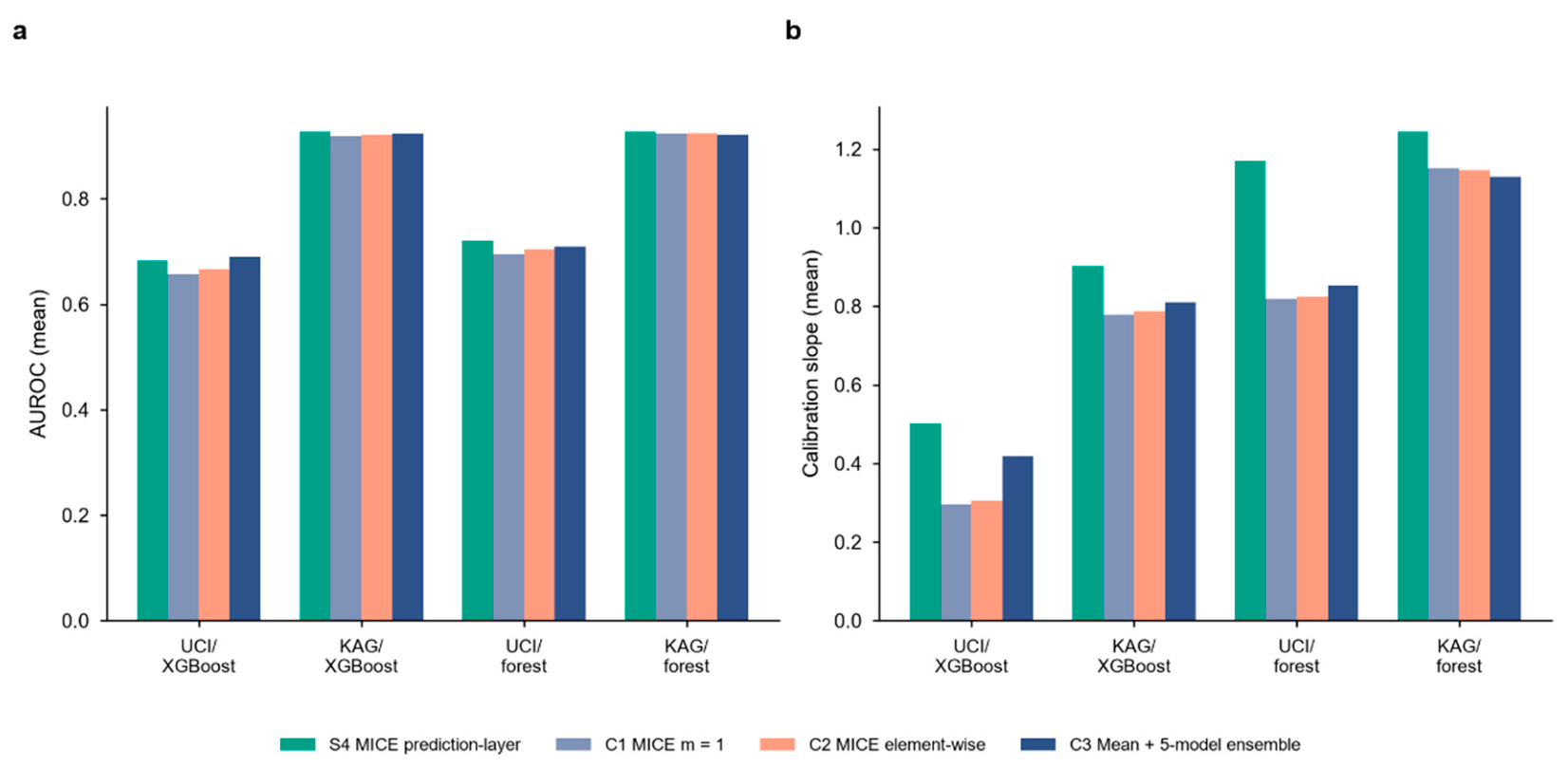
The decomposition clarifies the composition of the S4 advantage. The S4 advantage, when present, is not solely attributable to either multiple imputation or to prediction-layer averaging; it was probed by three matched contrasts, of which the smallest in our data is the MICE-specific increment; because C1/C2/C3 simultaneously change imputation count, model count, bootstrap resampling, and aggregation layer, the decomposition identifies candidate contributors rather than pure causal effects. For practitioners using tree learners on cohorts comparable in size to the smaller cohort studied here (n = 299), a 5-model bagged ensemble on a simple imputation may suffice for discrimination in the XGBoost setting specifically. For practitioners who need well-estimated probabilities, S4 prediction-layer pooling adds a methodologically sound descriptive Brier-score advantage across all four tested dataset-learner combinations, with slope improvement tracking the learner's under-fitting direction; the net-benefit analysis shows this improvement is descriptively higher than mean imputation across the plausible threshold range, while against a matched bagged ensemble the net-benefit margin is positive in the larger cohort only. The m-sensitivity arm shows these conclusions are not an artefact of choosing m = 5.
3.7. Cross-Cohort Rank Transferability Depends on Learner and on S4 MICE Consistency
Within each of the 9 matched conditions, strategy rankings (by mean AUROC) were compared between cohorts via Spearman correlation, separately for each learner (Figure 6). For cross-learner comparisons, the common-subset S1–S5 is used (S6 is L1-only); L1 rankings below use all 6 strategies and the interpretation is unchanged.
For L1 XGBoost, the mean rank correlation was ρ = +0.251 (range −0.43 to +0.94). S4 MICE was the best strategy in both cohorts in 4/9 conditions, driving the positive mean ρ; in the remaining conditions the best strategy differed between cohorts, reflecting the noisier rankings in the smaller cohort.
For L3 random forest, the mean ρ was +0.167 (range −0.50 to +0.90), with S4 MICE best in both cohorts in 5/9 conditions, the highest best-strategy concordance of any learner.
For L2 logistic regression, the mean ρ was −0.156 (range −0.60 to +0.70), with the best strategy agreeing across cohorts in only 1/9 conditions. This near-zero transferability is consistent with the near-zero between-strategy differences: when no strategy is meaningfully different, rankings are pure noise and cannot transfer.
Cross-cohort rank transferability has not previously been quantified across multiple learners in imputation research within the scope of our literature search. The learner-dependent pattern mirrors the discrimination results: where a true strategy effect exists (L1, L3, S4 MICE best), the best strategy agrees across cohorts in 4–5/9 conditions and mean rank correlation is positive; where no strategy effect was detected (L2), rankings are noise and do not transfer (mean ρ < 0). Transfer is far from perfect even for tree learners, mean ρ of 0.17–0.25 means the full ranking among near-equivalent non-MICE strategies is largely cohort-specific, and only the top position (S4) transfers with any reliability. This finding argues that reporting standards for imputation research should require multi-cohort evaluation with rank-transfer statistics, paralleling external-validation expectations for prediction models themselves (TRIPOD [5]; TRIPOD+AI [6]).
3.8. SHAP Explanation Stability Under Missingness
Explanation stability was quantified as the Spearman correlation between SHAP-based feature-importance rankings from imputed-data L1 XGBoost models and the complete-data reference, per condition and strategy, aggregated over 10 seeds (Figure 7; Table S2). This arm was run under the initial simulation release. Although the arm compares strategy-level stability within each mechanism rather than testing mechanism interactions, the change in masking protocol (age no longer masked under MAR) could alter SHAP values and rankings; the results should therefore be treated as exploratory evidence from an initial simulation release and not as definitive under the current design. Mean rank correlations were 0.75–0.96 across the 108 condition-strategy cells, with an overall mean of 0.88. Degradation increased with missingness rate (means 0.94/0.88/0.82 at 10/30/50%) and was worst under MNAR (mean 0.81 at 50% MNAR vs 0.83 at MCAR@50% and 0.82 at MAR@50%). The worst cell was UCI / MNAR@50% / S3 kNN (0.749). S2_Median was the least stable strategy (mean 0.867) and S4_MICE and S5_RF the joint most stable (both 0.889); the S5-minus-S2 advantage was directionally consistent but not significant under a paired Wilcoxon test across the 18 dataset-condition cells (mean difference +0.023, P = 0.094).
Because SHAP outputs increasingly inform clinical interpretation (for example, identifying medication burden and comorbidity as readmission drivers [15,16]) the stability of the explanation itself under realistic missingness is a safety-relevant property, yet it is rarely measured in cardiac-outcome prediction. Our results are double-edged. An overall mean of 0.88 suggests broad preservation of the global importance structure, which is reassuring for qualitative interpretation. However, correlations falling to the 0.75–0.81 range at 50% missingness imply that adjacent-ranked features swap order readily; for decisions that hinge on the relative weight of, say, renal function versus anaemia, such swaps are material. The pattern across mechanisms (MNAR worst) is consistent with the intuition that self-dependent missingness is most disruptive to feature-level explanations. Strategy-level differences were small (0.867–0.889) and the largest pairwise contrast (S5 vs S2) did not reach significance (P = 0.094); we therefore report explanation stability descriptively and do not claim a strategy ranking for it. We note that SHAP stability was assessed for L1 XGBoost only; the learner-dependence of explanation stability under imputation is an open question for future work. We propose that imputation comparisons (and any clinical deployment of explainable models on incomplete EHR) report explanation-stability statistics alongside discrimination and calibration.
3.9. MDD Analysis and Evaluation-Protocol Sensitivity
To assess whether non-significant Friedman tests might simply reflect insufficient power to detect differences of the observed magnitude, we computed the paired minimum detectable difference (MDD) for each S4-versus-alternative pair within each condition-learner combination, using the power-corrected formula MDD = (z₀.₉₇₅ + z₀.₈₀) · s_diff/√10 (Section 2.7; Table S3). The MDD approximates the smallest between-strategy AUROC difference detectable at α = 0.05 with 80% power given the observed per-seed paired variability; with only 10 seeds it is descriptive, not a formal equivalence bound. Dataset- and learner-specific median and maximum MDD values, the largest observed paired AUROC differences, and the numbers of comparisons exceeding their corresponding MDDs are summarised in Table 7.
Evaluation-protocol sensitivity. Because each per-seed AUROC is estimated on a single test fold (≈ 75 patients in UCI), we additionally concatenated test-fold predictions across the 10 seeds of each condition (L1 learner, both cohorts) and recomputed AUROC on the pooled predictions. The pooled protocol reproduced the per-seed strategy rankings exactly (rank Spearman ρ = 1.0 in both cohorts; Table S9), and the pooled S4-PL-minus-C3 differences matched the paired decomposition of Section 3.6. The per-seed evaluation protocol therefore did not determine the ranking conclusions.
The MDD analysis disciplines (but does not settle) the interpretation of null results. In Kaggle/L2 Logistic, no observed S4-versus-alternative difference exceeded its own MDD (0/36; observed maximum difference 0.003 against a median MDD of 0.003): with ten replicates this comparison is descriptive, and it does not suggest that the observed difference was merely too small to detect; because no equivalence bound was pre-specified and no two one-sided tests (TOST) procedure was performed, we report "no difference detected of practically relevant size" rather than proven equivalence. In Kaggle/L1 XGBoost, 29 of the 45 S4-versus-alternative comparisons exceeded their own MDD, consistent with the small but consistent S4 advantage being a detectable signal rather than noise. In UCI, the larger MDD values (0.025–0.062) reflect the small sample's higher variance, and the non-significant UCI results are best interpreted as inconclusive rather than as evidence of equivalence, a distinction we make explicit in the Limitations.
The four-arm decomposition (Section 3.6) provides additional MDD context: in UCI/L1, the S4-PL vs C3 difference (paired median −0.003) is far below the MDD (0.039), supporting the conclusion that the S4 discrimination advantage in that combination is below the detection threshold.
3.10. Correlated-Missingness Sensitivity
The main mechanisms generate masks independently across variables. To probe robustness of the strategy rank structure to multivariate, severity-driven missingness, a latent severity factor (first principal component of the continuous predictors) drove all masks jointly through a calibrated logistic link (Section 2.3; marginal rates exact: 0.100/0.301/0.500; Figure 8; Table S8). Because this arm implements a single missingness-generating scheme, it tests rank preservation, not the strategy × mechanism interaction, which is tested in Section 3.4. The results should be treated as exploratory evidence from an initial simulation release.
Figure 8.
Correlated-missingness sensitivity. Mean AUROC by strategy under independent missingness (main design, averaged over 27 cells) versus latent-severity correlated missingness (3 rates × 10 seeds), for the four dataset-learner combinations. Panel titles show the rank correlation between the two missingness schemes and the Friedman P for the strategy effect under correlated missingness. (Source data: correlated_missingness.csv, 660 records.).
Figure 8.
Correlated-missingness sensitivity. Mean AUROC by strategy under independent missingness (main design, averaged over 27 cells) versus latent-severity correlated missingness (3 rates × 10 seeds), for the four dataset-learner combinations. Panel titles show the rank correlation between the two missingness schemes and the Friedman P for the strategy effect under correlated missingness. (Source data: correlated_missingness.csv, 660 records.).
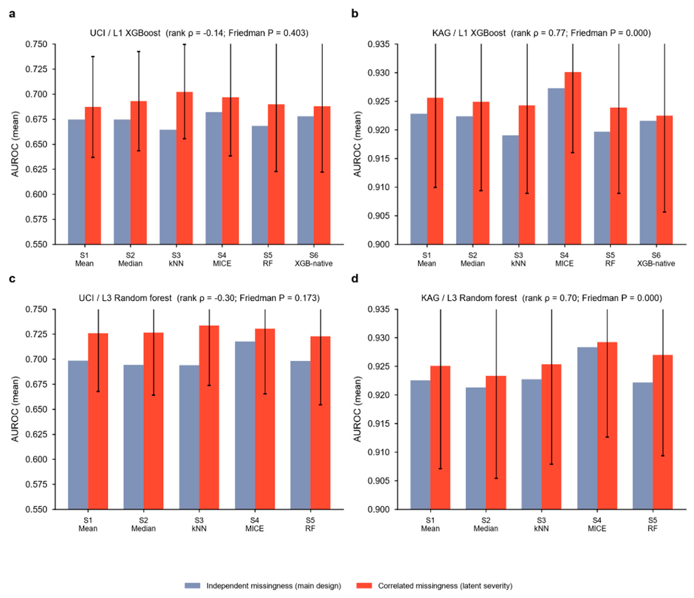
In the larger cohort, the strategy ranking under correlated missingness tracked the main-design ranking closely (Spearman ρ = 0.771 for Kaggle/L1, 0.700 for Kaggle/L3), S4 remained the top-ranked strategy at all three rates for L1 (and at 30–50% for L3), and the strategy effect remained significant (Friedman P = 2.3 × 10⁻⁴ and 5.8 × 10⁻⁵, respectively). In the small cohort, rankings did not transfer (ρ = −0.14 and −0.30) and no strategy effect was detectable (Friedman P = 0.400 and 0.170), mirroring the main design, where UCI comparisons were likewise MDD-limited (Section 3.9).
In the larger cohort, the learner-dependence pattern and the rank structure underlying the conclusion that mechanism tailoring lacks consistent support were also observed under correlated, value-dependent missingness wherever the design has adequate statistical power, and remained inconclusive exactly where they were already inconclusive. These results derive from an initial simulation release (see Limitation xvii) and require replication under the current protocol. The correlated-missingness arm also suggests that the marginal-rate calibration generalises beyond independent masks, though this too requires confirmation under the current protocol. What remains untested is real-world EHR missingness with hierarchical structure (panel ordering, care-process-driven patterns), which we flag as the priority for external replication (Section 4.5).
4. Discussion
4.1. Principal Findings
This leakage-controlled, dual-cohort simulation showed that the effect of imputation strategy varied across the three learner configurations tested. Prediction-layer-pooled multiple imputation by chained equations (S4) ranked first across all nine Kaggle conditions for XGBoost and random forest. In contrast, penalised logistic regression showed no Holm-confirmed strategy effect in either cohort. The exploratory Strategy × Learner interaction was significant in both cohorts, and targeted contrasts indicated that the pattern arose mainly from tree-versus-linear differences. However, these findings are conditional on two fixed cohorts, three learner configurations, and ten Monte Carlo replications.
Evidence for mechanism-tailored imputation was inconsistent. No Strategy × Mechanism interaction was detected in the larger Kaggle cohort, whereas the smaller UCI cohort showed interactions for the two tree learners. These interactions were unstable and did not replicate across cohorts. The results therefore do not support choosing an imputation strategy solely from an assumed MCAR, MAR, or MNAR classification. Correlated-missingness sensitivity analysis preserved the strategy ranking in the larger cohort, although this analysis used the initial simulation protocol and requires confirmation under the revised workflow. Cross-cohort rank transferability was modest for the tree learners and absent for logistic regression, indicating that strategy rankings should not be assumed to transfer between datasets.
4.2. Decomposition and Interpretation
The four-arm comparison showed that the S4 advantage was not attributable solely to multiple imputation. Averaging predictions from multiple fitted models reduced variance and was statistically indistinguishable from the full discrimination advantage in the small-cohort XGBoost analysis, and accounted for part of the advantage in the other combinations. After comparison with a matched bagged-mean control, the remaining S4 increment was significant in three of four dataset-learner combinations but small in absolute terms, with paired median AUROC differences of approximately 0.005–0.007. Prediction-layer pooling also performed better than element-wise averaging in three combinations, with the same direction in the fourth. These matched comparisons identify plausible contributors to the observed advantage but do not isolate pure causal mechanisms.
The results are consistent with a bias-variance interpretation. Prediction averaging should benefit learners with greater sampling variance, such as tree ensembles, while having less effect on a relatively low-variance penalised logistic model [59]. The targeted S4 contrast was null for logistic regression, whereas an increment over the matched bagged control remained in both random-forest analyses and in Kaggle XGBoost. No additional increment was detected for UCI XGBoost, where bagging after mean imputation matched the pooled-MICE arm within the resolution of the paired comparison. This interpretation was not tested through a formal bias-variance decomposition or systematic manipulation of model complexity and should therefore be regarded as a plausible explanation rather than an established mechanism.
Probability estimation showed a related but more qualified pattern. S4 had the lowest mean Brier score in all four dataset-learner combinations, although no seed-level paired test was performed for this outcome. Calibration-slope changes depended on the direction of the original miscalibration: pooling moved slopes toward one for under-fitted XGBoost models but not for random forests whose slopes already exceeded one. Decision-curve net benefit was higher than mean imputation across the examined thresholds, but the curves reused patients across seeds and conditions and were not independently validated. The calibration and decision-curve findings should therefore be interpreted descriptively.
4.3. Relation to Previous Work
The learner-dependent pattern may help reconcile conflicting recommendations in the literature. Studies reporting an advantage for MICE often used tree-based or ensemble learners without separating multiple-imputation effects from generic ensemble averaging [14,15]. Studies concluding that simple imputation was sufficient more often used regularised linear or parametric models [12,56]. These studies may have identified local optima that depended on the learner, dataset, and evaluation protocol rather than universally superior strategies.
Evidence from other clinical domains supports this interpretation. In dementia classification, the preferred strategy differed between random forest, logistic regression, and support vector machines [22]. MissForest ranked highly in diabetes and mixed healthcare datasets evaluated mainly under MCAR assumptions and with imputation-accuracy outcomes [23,24]. Deep-learning methods that model missingness directly provide another option, but their trade-offs relative to conventional impute-then-fit workflows were outside the present study [25].
The two cohorts should not be interpreted as external validations of the same outcome. UCI assessed death during heart-failure follow-up, whereas Kaggle assessed structural heart-disease classification. Comparisons with the heart-failure literature therefore rest primarily on UCI and on broader learner-level principles. Absolute performance and calibration findings remain task-specific.
4.4. Practical Implications and Future Work
For tree-based learners, prediction-layer-pooled MICE is a reasonable candidate for sensitivity analysis when probability estimation matters. Its discrimination advantage over matched bagging was small, and the evidence does not justify treating it as a validated clinical default. For small-cohort XGBoost, bagging after simple imputation reproduced the observed discrimination benefit, although this result did not extend to random forest. Logistic regression showed no Holm-confirmed condition-level advantage for any strategy. These findings support evaluating imputation jointly with the downstream learner rather than selecting it as an isolated preprocessing step.
Complete-case analysis became severely sample-limited as missingness increased and was often untrainable at 50% missingness in the smaller cohort. Where it remained feasible under MAR, it evaluated a selected, lower-risk subgroup and was not directly comparable with full-fold imputation. Calibration should also be assessed before threshold-based use. In the single repair analysis performed, tuning followed by Platt calibration substantially improved the UCI XGBoost calibration slope, but this result requires replication across learners and missing-data settings.
Future work should first evaluate mean imputation with missingness indicators, a common clinical comparator omitted here. The complete protocol should then be replicated in cohorts with real, hierarchically structured missingness, such as MIMIC-IV. Expanding the learner panel to gradient-boosting variants and neural networks would test whether the proposed bias-variance account predicts effects across model classes. Finally, imputation strategies should be evaluated across sex, age, and other clinically relevant subgroups because missing-data handling may alter performance disparities [27].
4.5. Limitations
Missingness was simulated and may not represent hierarchical, care-process-driven patterns in real electronic health records [60]. Only continuous variables were masked; categorical, longitudinal, and time-varying missingness were not examined. The correlated-missingness analysis also relied on unverifiable assumptions.
The cohorts differed in size and outcome. UCI evaluated mortality during heart-failure follow-up, whereas Kaggle evaluated structural heart-disease classification. Findings should therefore not be transferred uncritically between tasks. The small UCI sample limited power, and non-significant results do not establish equivalence. The ten seeds represent Monte Carlo replications rather than independent clinical samples.
Several analyses had restricted scope. XGBoost-native handling and SHAP stability were evaluated only with XGBoost, while the four-arm decomposition excluded logistic regression. Models used fixed hyperparameters, and calibration repair was tested only on complete UCI data. Missingness indicators, deep imputation, nonlinear calibration, and subgroup fairness were not evaluated; a subgroup-fairness assessment was not feasible here because neither source dataset provides sociodemographic variables beyond age and sex, and the UCI test fold (n ≈ 75; ≈ 24 events) cannot support a subgroup analysis. Two implementation choices bound the reading of the strategy comparison. Features were not standardised, so the kNN imputer selected neighbours under a raw-scale distance metric in which wide-range laboratory variables dominate; a scaled variant could rank the strategies differently. The five nominal Kaggle variables entered as ordinal integers for all learners, so the linear learner could exploit an ordering absent from the categories; the conclusion that the penalised logistic regression showed no strategy effect may be specific to this encoding. Neither choice was varied in the factorial design, so both are potential effect modifiers that the present comparison does not resolve.
Some sensitivity analyses used the initial simulation protocol and require confirmation under the revised protocol. Repeated-measures ANOVA results lacked sphericity correction and remain exploratory; the interaction terms reported in Table 4 form a family of tests that received no multiplicity control and should not be read as confirmatory. Decision-curve analyses were descriptive because patients were reused across seeds and conditions. No prospective power analysis was conducted, and the complete workflow has not been rerun from a clean environment. These limitations restrict population-level and clinical generalisation.
5. Conclusions
In two public cardiac prediction tasks (HF follow-up mortality (UCI) and structural heart disease classification (Kaggle)) the effect of imputation strategy on discrimination differed across the three learner configurations tested: S4 MICE with prediction-layer pooling ranked first for the two tree-based learners (XGBoost, random forest) in all 9 Kaggle conditions, while the penalised logistic regression showed no Holm-confirmed strategy effect. The exploratory omnibus Strategy × Learner interaction was significant in both cohorts (repeated-measures ANOVA, not sphericity-corrected); targeted Wilcoxon contrasts localised the effect primarily to tree-versus-linear comparisons. No consistent strategy × mechanism interaction was found (absent in the larger cohort, non-replicating in the small cohort) giving no support for mechanism-tailored imputation. A four-arm decomposition showed that the S4 discrimination advantage is partly a generic ensemble effect, with a MICE-specific increment that is small (paired median ≤ +0.007 AUROC) and not detected in the small-cohort XGBoost combination. Brier score was descriptively lowest under S4 in all four dataset-learner combinations (no seed-level paired inference). More broadly, we suggest that imputation advances most reliably when evaluated and reported jointly with the downstream learner, with any advantage separated into ensemble-level and imputation-specific components and judged against explicit detectability limits, so that conclusions rest on effects that survive across cohorts, learners, and missingness regimes rather than on the setting that produced them.
Supplementary Materials
The following supporting information can be downloaded at the website of this paper posted on Preprints.org. The following supporting information accompanies this article and is supplied as separate files. Supplementary Tables S1–S12 are provided in the single workbook Supplementary_Tables.xlsx, whose sheet names correspond to the table numbers used below. Table S1. Strategy-level AUROC, AUPRC, Brier, slope and E_avg (mean ± s.d.) for each of the 54 conditions, by learner. Table S2. SHAP feature-rank stability (Spearman ρ) by strategy and condition, L1 XGBoost, 10 seeds. Table S3. Paired minimum detectable difference (MDD) for each strategy pair, by condition and learner. Table S4. Four-arm decomposition, paired Wilcoxon tests with Holm correction, paired median differences with 95% percentile bootstrap intervals, and per-condition Friedman tests. Table S5. Strategy × condition AUPRC by learner (full grid). Table S6. Leakage sensitivity, UCI complete-data AUROC with vs. without time variable, 10 seeds. With time: 0.910 ± 0.030; without time: 0.713 ± 0.041. Table S7. Complete-case analysis, feasibility (complete rows per partition) and performance by condition and learner. Table S8. Correlated-missingness arm, strategy-level metrics by rate and learner, with rank correlations versus the main design. Table S9. Pooled-prediction AUROC versus per-seed AUROC by condition (L1 learner, both cohorts). Table S10. (a) Calibration-repair sensitivity (UCI/L1, complete data); (b) MICE convergence diagnostics; (c) decision-curve net benefit at representative thresholds with 10–90% condition bands; (d) MICE m-sensitivity (m ∈ {5, 10, 20}). Table S11. Empirical marginal missingness rates by mechanism and nominal rate (10 seeds, both cohorts). Table S12. (a) Omnibus Strategy × Learner repeated-measures ANOVA per cohort (seed-aggregated); (b) pre-specified targeted (S4−S1) learner-pair contrasts (seed-aggregated, n = 10, Holm-corrected); (c) Strategy × Mechanism × Learner three-way repeated-measures interaction per cohort; (d) three-way repeated-measures ANOVA per dataset–learner combination (the full models underlying Table 4).
Author Contributions
Conceptualization, L.L.; methodology, L.L.; software, M.L.; formal analysis, M.L.; investigation, M.L.; data curation, M.L.; visualization, M.L.; writing—original draft preparation, M.L.; writing—review and editing, L.L.; supervision, L.L.; funding acquisition, L.L. All authors have read and agreed to the published version of the manuscript.
Funding
This research was funded by the Department of Education of Anhui Province, grant number 2025AHGXZK20080.
Institutional Review Board Statement
Not applicable. This study is a secondary analysis of two publicly available, fully de-identified datasets distributed under open licences; no new human-subject data were collected.
Informed Consent Statement
Not applicable. This secondary analysis used publicly available, de-identified datasets.
Data Availability Statement
The UCI Heart Failure Clinical Records dataset is available from the UCI Machine Learning Repository at https://doi.org/10.24432/C5Z89R under the Creative Commons Attribution 4.0 International (CC BY 4.0) licence. The Kaggle Heart Failure Prediction dataset is available at https://doi.org/10.34740/KAGGLE/DS/2162210 under the Open Data Commons Open Database License (ODbL) v1.0. Both datasets are redistributed unmodified, under their original licences, inside the reproduction archive so that a single command reproduces every reported result. The archive contains all analysis code, raw record files (CSV), prediction stores, the environment manifest, a single-entry reproduction script, SHA-256 checksums, figure-generation scripts and the staged analysis-plan files, and is openly archived on Zenodo (concept DOI: 10.5281/zenodo.23274933; version DOI: 10.5281/zenodo.23276666). The analysis code is released under the MIT licence; this licence applies to the code only and does not alter the licences of the two source datasets, which remain as stated above. No new data were generated in this study.
Declaration of AI-Assisted Technologies
During the preparation of this work, the authors used AI-assisted tools solely for language editing and copy-editing, and not for the generation of scientific content, the design of the study, the analysis of data, or the interpretation of results. All AI-assisted outputs were reviewed and verified by the authors against the raw analysis records and the underlying statistical outputs, and the authors edited and approved the final text and take full responsibility for the content of the publication.
Conflicts of Interest
The authors declare no conflict of interest.
References
- Savarese, G.; Lund, L.H. Global Public Health Burden of Heart Failure. Card. Fail. Rev. 2017, 3, 7. [CrossRef]
- Desai, A.S.; Stevenson, L.W. Rehospitalization for Heart Failure. Circulation 2012, 126, 501–506. [CrossRef]
- Hajishah, H.; Kazemi, D.; Safaee, E.; Amini, M.J.; Peisepar, M.; Tanhapour, M.M.; et al. Evaluation of Machine Learning Methods for Prediction of Heart Failure Mortality and Readmission: Meta-Analysis. BMC Cardiovasc. Disord. 2025, 25, 264. [CrossRef]
- Van Calster, B.; McLernon, D.J.; van Smeden, M.; Wynants, L.; Steyerberg, E.W. Calibration: The Achilles Heel of Predictive Analytics. BMC Med. 2019, 17, 230. [CrossRef]
- Collins, G.S.; Reitsma, J.B.; Altman, D.G.; Moons, K.G.M. Transparent Reporting of a Multivariable Prediction Model for Individual Prognosis or Diagnosis (TRIPOD): The TRIPOD Statement. BMJ 2015, 350, g7594. [CrossRef]
- Collins, G.S.; Moons, K.G.M. TRIPOD+AI Statement: Updated Guidance for Reporting Clinical Prediction Models That Use Regression or Machine Learning Methods. BMJ 2024, 385, e078378. [CrossRef]
- Alba, A.C.; Agoritsas, T.; Walsh, M.; Hanna, S.; Iorio, A.; Devereaux, P.J.; McGinn, T.; Guyatt, G. Discrimination and Calibration of Clinical Prediction Models. JAMA 2017, 318, 1377–1385. [CrossRef]
- Pedersen, A.B.; Mikkelsen, E.M.; Cronin-Fenton, D.; Kristensen, N.R.; Pham, T.M.; Pedersen, L.; et al. Missing Data and Multiple Imputation in Clinical Epidemiological Research. Clin. Epidemiol. 2017, 9, 157–166. [CrossRef]
- Janssen, K.J.M.; Donders, A.R.T.; Harrell, F.E., Jr.; Vergouwe, Y.; Chen, Q.; Grobbee, D.E.; et al. Missing Covariate Data in Medical Research: To Impute Is Better Than to Ignore. J. Clin. Epidemiol. 2010, 63, 721–727. [CrossRef]
- Troyanskaya, O.; Cantor, M.; Sherlock, G.; Brown, P.; Hastie, T.; Tibshirani, R.; Botstein, D.; Altman, R.B. Missing Value Estimation Methods for DNA Microarrays. Bioinformatics 2001, 17, 520–525. [CrossRef]
- Stekhoven, D.J.; Bühlmann, P. MissForest—Non-Parametric Missing Value Imputation for Mixed-Type Data. Bioinformatics 2012, 28, 112–118. [CrossRef]
- van Buuren, S. Flexible Imputation of Missing Data, 2nd ed.; Chapman & Hall/CRC: Boca Raton, FL, USA, 2018. [CrossRef]
- Emmanuel, T.; Maupong, T.; Mpoeleng, D.; Semong, T.; Mphago, B.; Tabona, O. A Survey on Missing Data in Machine Learning. J. Big Data 2021, 8, 140. [CrossRef]
- Hidayaturrohman, Q.A.; Hanada, E. Impact of Data Pre-Processing Techniques on XGBoost Model Performance for Predicting All-Cause Readmission and Mortality among Patients with Heart Failure. BioMedInformatics 2024, 4, 2201–2212. [CrossRef]
- Shin, I.; Bhatt, N.; Alashi, A.; Kandala, K.; Murugiah, K. Predicting 30-Day and 1-Year Mortality in Heart Failure with Preserved Ejection Fraction (HFpEF). PLoS ONE 2025, 20, e0336809. [CrossRef]
- Jiang, M.H.; Yu, F.; Yang, H.Y.; Yin, S.J.; Yang, L.J.; Chen, Y.; et al. Predicting Readmission Rates in Critically Ill Heart Failure Patients during a 90-Day Vulnerable Phase Using Interpretable Machine Learning Models. Clinics 2025, 80, 100775. [CrossRef]
- Rubin, D.B. Inference and Missing Data. Biometrika 1976, 63, 581–592. [CrossRef]
- Little, R.J.A.; Rubin, D.B. Statistical Analysis with Missing Data, 3rd ed.; Wiley: Hoboken, NJ, USA, 2019. [CrossRef]
- Wood, A.M.; White, I.R.; Royston, P. How Should Variable Selection Be Performed with Multiply Imputed Data? Stat. Med. 2008, 27, 3227–3246. [CrossRef]
- White, I.R.; Royston, P. Imputing Missing Covariate Values for the Cox Model. Stat. Med. 2009, 28, 1982–1998. [CrossRef]
- Audigier, V.; White, I.R.; Jolani, S.; Debray, T.P.A.; Quartagno, M.; Carpenter, J.; et al. Multiple Imputation for Multilevel Data with Continuous and Binary Variables. Stat. Sci. 2018, 33, 160–183. [CrossRef]
- Aracri, F.; Bianco, M.G.; Quattrone, A.; Sarica, A. Bridging the Gap: Missing Data Imputation Methods and Their Effect on Dementia Classification Performance. Brain Sci. 2025, 15, 639. [CrossRef]
- Tiwaskar, S.; Rashid, M.; Gokhale, P. Impact of Machine Learning-Based Imputation Techniques on Medical Datasets: A Comparative Analysis. Multimed. Tools Appl. 2025, 84, 5905–5925. [CrossRef]
- Joel, L.O.; Doorsamy, W.; Paul, B.S. A Comparative Study of Imputation Techniques for Missing Values in Healthcare Diagnostic Datasets. Int. J. Data Sci. Anal. 2025, 20, 6357–6373. [CrossRef]
- Caruso, C.M.; Guarrasi, V.; Ramella, S.; Soda, P. A Deep Learning Approach for Overall Survival Prediction in Lung Cancer with Missing Values. Comput. Methods Programs Biomed. 2024, 254, 108308. [CrossRef]
- Yoon, J.; Jordon, J.; van der Schaar, M. GAIN: Missing Data Imputation Using Generative Adversarial Nets. In Proceedings of the 35th International Conference on Machine Learning (ICML), Stockholm, Sweden, 10–15 July 2018; PMLR: 2018; Volume 80, pp. 5689–5698.
- Cirillo, D.; Catuara-Solarz, S.; Morey, C.; Guney, E.; Subirats, L.; Mellino, S.; Gigante, A.; Valencia, A.; Rementeria, M.J.; Chadha, A.S.; et al. Sex and Gender Differences and Biases in Artificial Intelligence for Biomedicine and Healthcare. npj Digit. Med. 2020, 3, 81. [CrossRef]
- Wongyikul, P.; Jirattikanwong, N.; Isaradech, N.; Kiratipaisarl, W.; Phrommintikul, A.; Sirikul, W.; Phinyo, P. Comparing Imputation Methods for Clinical Prediction Model Development under Complex Missingness Scenarios: A Simulation Study Using Real-World Cardiac Data. arXiv 2026, arXiv:2607.07247. [CrossRef]
- Chicco, D.; Jurman, G. Machine Learning Can Predict Survival of Patients with Heart Failure from Serum Creatinine and Ejection Fraction Alone. BMC Med. Inform. Decis. Mak. 2020, 20, 16. [CrossRef]
- Heart Failure Clinical Records [Dataset]; UCI Machine Learning Repository: Irvine, CA, USA, 2020. (CC BY 4.0.). [CrossRef]
- Harrell, F.E., Jr. Regression Modeling Strategies: With Applications to Linear Models, Logistic and Ordinal Regression, and Survival Analysis, 2nd ed.; Springer: Cham, Switzerland, 2015. [CrossRef]
- Peduzzi, P.; Concato, J.; Kemper, E.; Holford, T.R.; Feinstein, A.R. A Simulation Study of the Number of Events per Variable in Logistic Regression Analysis. J. Clin. Epidemiol. 1996, 49, 1373–1379. [CrossRef]
- fedesoriano. Heart Failure Prediction Dataset [Dataset]; Kaggle: San Francisco, CA, USA, 2021. Available online: https://www.kaggle.com/datasets/fedesoriano/heart-failure-prediction (accessed on 6 September 2026). Distributed under the Open Data Commons Open Database License (ODbL) v1.0.
- Suissa, S. Immortal Time Bias in Pharmacoepidemiology. Am. J. Epidemiol. 2008, 167, 492–499. [CrossRef]
- Rubin, D.B. Multiple Imputation for Nonresponse in Surveys; John Wiley & Sons: New York, NY, USA, 1987. [CrossRef]
- Marshall, A.; Altman, D.G.; Holder, R.L.; Royston, P. Combining Estimates of Interest in Prognostic Modelling Studies after Multiple Imputation: Current Practice and Guidelines. BMC Med. Res. Methodol. 2009, 9, 57. [CrossRef]
- Sterne, J.A.C.; White, I.R.; Carlin, J.B.; Spratt, M.; Royston, P.; Kenward, M.G.; Wood, A.M.; Carpenter, J.R. Multiple Imputation for Missing Data in Epidemiological and Clinical Research: Potential and Pitfalls. BMJ 2009, 338, b2393. [CrossRef]
- van Buuren, S.; Groothuis-Oudshoorn, K. Mice: Multivariate Imputation by Chained Equations in R. J. Stat. Softw. 2011, 45, 1–67. [CrossRef]
- Azur, M.J.; Stuart, E.A.; Frangakis, C.; Leaf, P.J. Multiple Imputation by Chained Equations: What Is It and How Does It Work? Int. J. Methods Psychiatr. Res. 2011, 20, 40–49. [CrossRef]
- Chen, T.; Guestrin, C. XGBoost: A Scalable Tree Boosting System. In Proceedings of the 22nd ACM SIGKDD International Conference on Knowledge Discovery and Data Mining, San Francisco, CA, USA, 13–17 August 2016; ACM: New York, NY, USA, 2016; pp. 785–794. [CrossRef]
- Petmezas, G.; Papageorgiou, V.E.; Vassilikos, V.; Pagourelias, E.; Tachmatzidis, D.; Tsaklidis, G.; et al. Enhanced Heart Failure Mortality Prediction through Model-Independent Hybrid Feature Selection and Explainable Machine Learning. J. Biomed. Inform. 2025, 163, 104800. [CrossRef]
- Friedman, J.; Hastie, T.; Tibshirani, R. Regularization Paths for Generalized Linear Models via Coordinate Descent. J. Stat. Softw. 2010, 33, 1–22. [CrossRef]
- Breiman, L. Random Forests. Mach. Learn. 2001, 45, 5–32. [CrossRef]
- Saito, T.; Rehmsmeier, M. The Precision-Recall Plot Is More Informative than the ROC Plot When Evaluating Binary Classifiers on Imbalanced Datasets. PLoS ONE 2015, 10, e0118432. [CrossRef]
- Van Calster, B.; Nieboer, D.; Vergouwe, Y.; De Cock, B.; Pencina, M.J.; Steyerberg, E.W. A Calibration Hierarchy for Risk Models Was Defined: From Utopia to Empirical Data. J. Clin. Epidemiol. 2016, 74, 167–176. [CrossRef]
- Austin, P.C.; Steyerberg, E.W. The Integrated Calibration Index (ICI) and Related Metrics for Quantifying the Calibration of Logistic Regression Models. Stat. Med. 2019, 38, 4051–4065. [CrossRef]
- Vickers, A.J.; Elkin, E.B. Decision Curve Analysis: A Novel Method for Evaluating Prediction Models. Med. Decis. Mak. 2006, 26, 565–574. [CrossRef]
- Vickers, A.J.; Cronin, A.M.; Elkin, E.B.; Gonen, M. Extensions to Decision Curve Analysis, a Novel Method for Evaluating Diagnostic Tests, Prediction Models and Molecular Markers. BMC Med. Inform. Decis. Mak. 2008, 8, 53. [CrossRef]
- Lundberg, S.M.; Lee, S.-I. A Unified Approach to Interpreting Model Predictions. In Advances in Neural Information Processing Systems 30 (NIPS 2017), Long Beach, CA, USA, 4–9 December 2017; Curran Associates, Inc.: Red Hook, NY, USA, 2017; pp. 4765–4774.
- Wilcoxon, F. Individual Comparisons by Ranking Methods. Biom. Bull. 1945, 1, 80–83. [CrossRef]
- Friedman, M. The Use of Ranks to Avoid the Assumption of Normality Implicit in the Analysis of Variance. J. Am. Stat. Assoc. 1937, 32, 675–701. [CrossRef]
- Demšar, J. Statistical Comparisons of Classifiers over Multiple Data Sets. J. Mach. Learn. Res. 2006, 7, 1–30.
- Holm, S. A Simple Sequentially Rejective Multiple Test Procedure. Scand. J. Stat. 1979, 6, 65–70.
- Gelman, A.; Stern, H. The Difference between “Significant” and “Not Significant” Is Not Itself Statistically Significant. Am. Stat. 2006, 60, 328–331. [CrossRef]
- Wolff, R.F.; Moons, K.G.M.; Riley, R.D.; Whiting, P.F.; Westwood, M.; Collins, G.S.; et al. PROBAST: A Tool to Assess the Risk of Bias and Applicability of Prediction Model Studies. Ann. Intern. Med. 2019, 170, 51–58. [CrossRef]
- Gao, Z.; Xu, Y.; Wu, W.; Wang, X.; Kong, Y.; Tian, T. Towards Better Clinical Prediction and Interpretation via a New Imputation Strategy from National Health and Nutrition Examination Survey. Stat. Interface 2024, 17, 425–437. [CrossRef]
- Cawley, G.C.; Talbot, N.L.C. On Over-Fitting in Model Selection and Subsequent Selection Bias in Performance Evaluation. J. Mach. Learn. Res. 2010, 11, 2079–2107.
- Niculescu-Mizil, A.; Caruana, R. Predicting Good Probabilities with Supervised Learning. In Proceedings of the 22nd International Conference on Machine Learning (ICML ’05), Bonn, Germany, 7–11 August 2005; ACM: New York, NY, USA, 2005; pp. 625–632. [CrossRef]
- Hastie, T.; Tibshirani, R.; Friedman, J. The Elements of Statistical Learning: Data Mining, Inference, and Prediction, 2nd ed.; Springer: New York, NY, USA, 2009. [CrossRef]
- Agniel, D.; Kohane, I.S.; Weber, G.M. Biases in Electronic Health Record Data Due to Processes within the Healthcare System: Retrospective Observational Study. BMJ 2018, 361, k1479. [CrossRef]
Figure 1.
Study design and strategy implementations. (a) Two-cohort, full-factorial simulation design with three learners. (b) The six imputation strategies; S4 MICE pools at the prediction layer (five models trained, probabilities averaged). S7 (complete-case) and C1–C3 are reference/control arms analysed in Section 3.2 and Section 3.6.
Figure 1.
Study design and strategy implementations. (a) Two-cohort, full-factorial simulation design with three learners. (b) The six imputation strategies; S4 MICE pools at the prediction layer (five models trained, probabilities averaged). S7 (complete-case) and C1–C3 are reference/control arms analysed in Section 3.2 and Section 3.6.
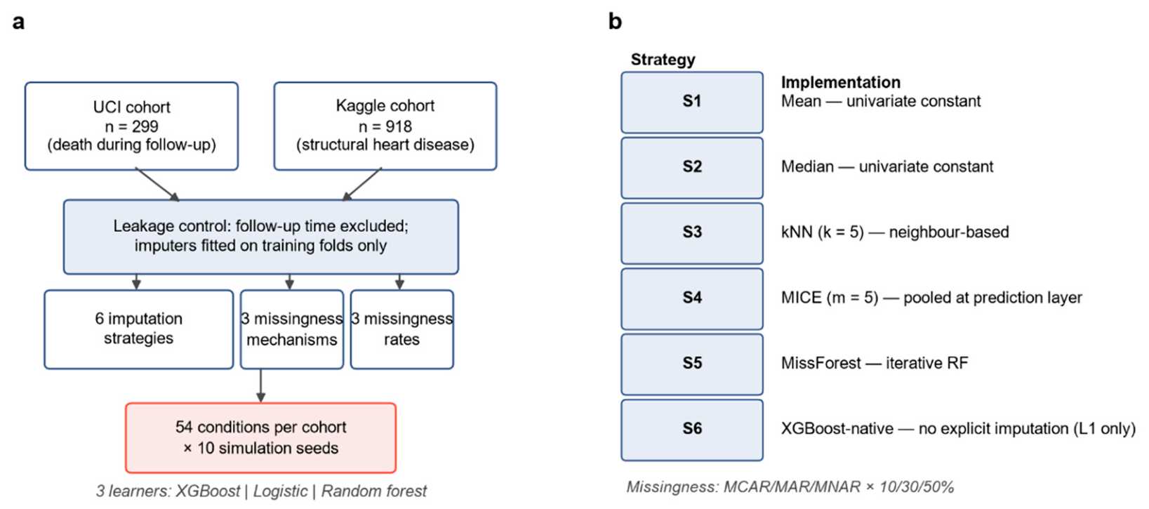
Figure 2.
Discrimination across 54 conditions, stratified by learner. (a, b) Strategy × condition AUROC heatmaps for UCI and Kaggle (L1 XGBoost, 6 strategies). (c, d) AUROC as a function of missingness rate, stratified by mechanism; error bars are 1 s.d. across 10 seeds (L1). (e, f) Corresponding heatmaps for L3 random forest (5 strategies; S6 only L1). Dotted lines mark complete-data performance. (Source data: main_results_full.csv, 2,940 records; MCAR conditions from the initial release, MAR/MNAR from the rewritten simulation, Section 2.3.).
Figure 2.
Discrimination across 54 conditions, stratified by learner. (a, b) Strategy × condition AUROC heatmaps for UCI and Kaggle (L1 XGBoost, 6 strategies). (c, d) AUROC as a function of missingness rate, stratified by mechanism; error bars are 1 s.d. across 10 seeds (L1). (e, f) Corresponding heatmaps for L3 random forest (5 strategies; S6 only L1). Dotted lines mark complete-data performance. (Source data: main_results_full.csv, 2,940 records; MCAR conditions from the initial release, MAR/MNAR from the rewritten simulation, Section 2.3.).
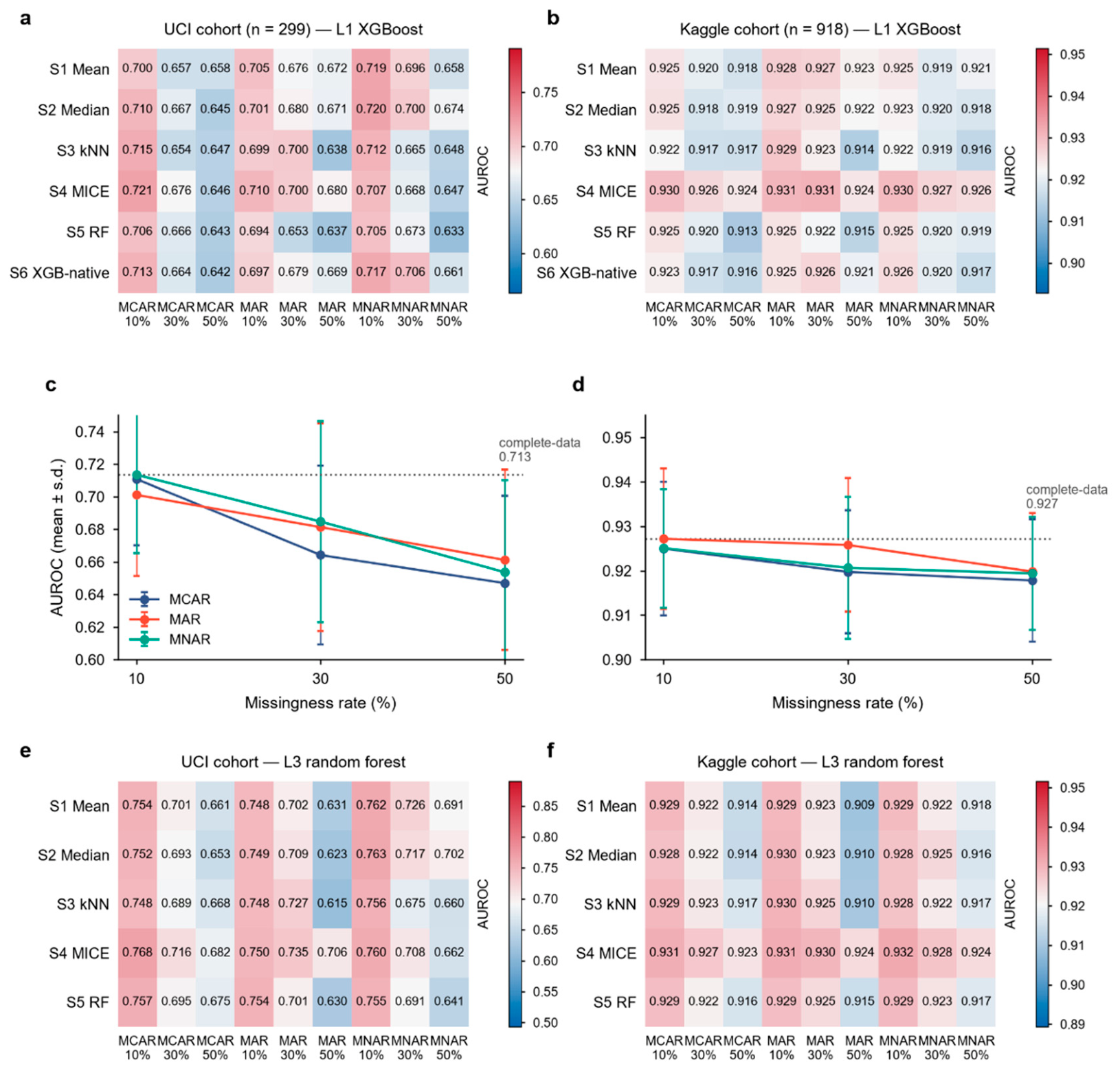
Figure 3.
Strategy profiles across missingness mechanisms, all six dataset-learner combinations. (a, b) L1 XGBoost; (c, d) L2 logistic regression; (e, f) L3 random forest (UCI left, Kaggle right). Mean AUROC by strategy and mechanism; curves close to parallel indicate absence of strategy × mechanism interaction. F/P values derive from the repeated-measures Strategy × Mechanism terms in Table 4.
Figure 3.
Strategy profiles across missingness mechanisms, all six dataset-learner combinations. (a, b) L1 XGBoost; (c, d) L2 logistic regression; (e, f) L3 random forest (UCI left, Kaggle right). Mean AUROC by strategy and mechanism; curves close to parallel indicate absence of strategy × mechanism interaction. F/P values derive from the repeated-measures Strategy × Mechanism terms in Table 4.
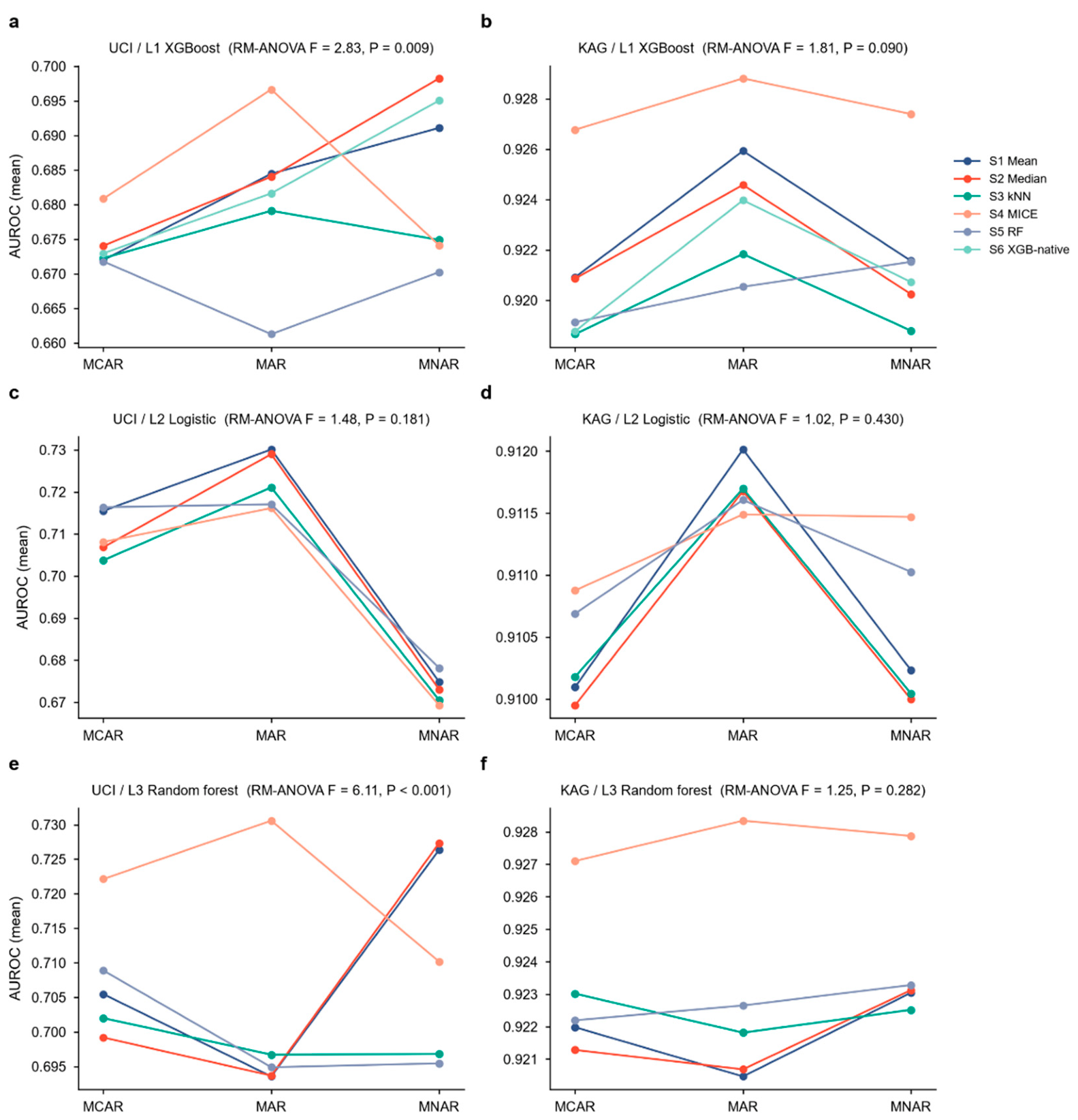
Figure 4.
Calibration across strategies and conditions. (a, b) Calibration slope heatmaps for UCI and Kaggle (L1 XGBoost); an ideal slope is 1.0 (white). UCI is broadly over-confident (slope < 0.5 for most strategies), while Kaggle approaches ideal. (c) Calibration curves under MNAR, 30% missingness, pooled across 10 seeds for L1 XGBoost; solid lines (Kaggle), dashed lines (UCI). (Source data: main_results_full.csv and the prediction stores.).
Figure 4.
Calibration across strategies and conditions. (a, b) Calibration slope heatmaps for UCI and Kaggle (L1 XGBoost); an ideal slope is 1.0 (white). UCI is broadly over-confident (slope < 0.5 for most strategies), while Kaggle approaches ideal. (c) Calibration curves under MNAR, 30% missingness, pooled across 10 seeds for L1 XGBoost; solid lines (Kaggle), dashed lines (UCI). (Source data: main_results_full.csv and the prediction stores.).
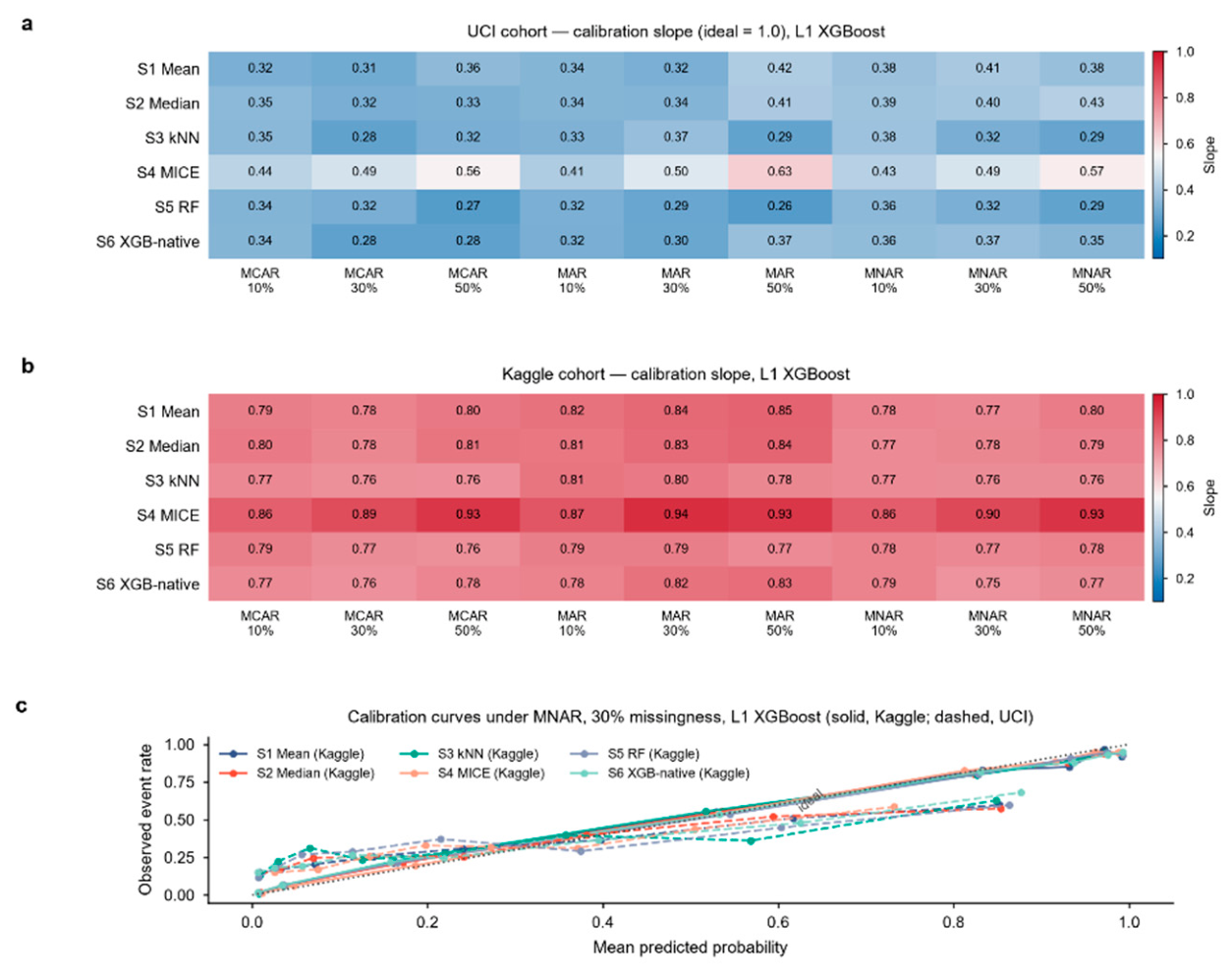
Figure 6.
Cross-cohort rank transferability, by learner. (a) Per-condition Spearman ρ between the 6-strategy (L1) or 5-strategy (L2, L3) AUROC rankings in UCI and Kaggle, for each of the 9 missingness conditions (3 learners, grouped bars). (b-d) Per-strategy mean rank within each cohort, slopegraph for L1, L2, L3. S4 MICE is the consistent leader for L1 and L3; rankings for L2 are noise-level. Cross-learner comparisons use the S1–S5 common subset.
Figure 6.
Cross-cohort rank transferability, by learner. (a) Per-condition Spearman ρ between the 6-strategy (L1) or 5-strategy (L2, L3) AUROC rankings in UCI and Kaggle, for each of the 9 missingness conditions (3 learners, grouped bars). (b-d) Per-strategy mean rank within each cohort, slopegraph for L1, L2, L3. S4 MICE is the consistent leader for L1 and L3; rankings for L2 are noise-level. Cross-learner comparisons use the S1–S5 common subset.
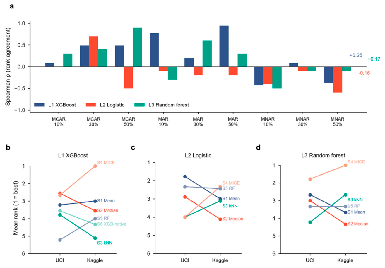
Figure 7.
SHAP-based feature-importance stability under missingness (L1 XGBoost, 10 seeds). (a, b) Spearman ρ between the SHAP feature-importance ranking of the imputed-data model and the complete-data reference, across the 54-condition grid for UCI and Kaggle. The minimum is 0.75 (UCI / MNAR@50% / S3); S4_MICE and S5_RF are the joint most stable strategies, S2_Median the least.
Figure 7.
SHAP-based feature-importance stability under missingness (L1 XGBoost, 10 seeds). (a, b) Spearman ρ between the SHAP feature-importance ranking of the imputed-data model and the complete-data reference, across the 54-condition grid for UCI and Kaggle. The minimum is 0.75 (UCI / MNAR@50% / S3); S4_MICE and S5_RF are the joint most stable strategies, S2_Median the least.
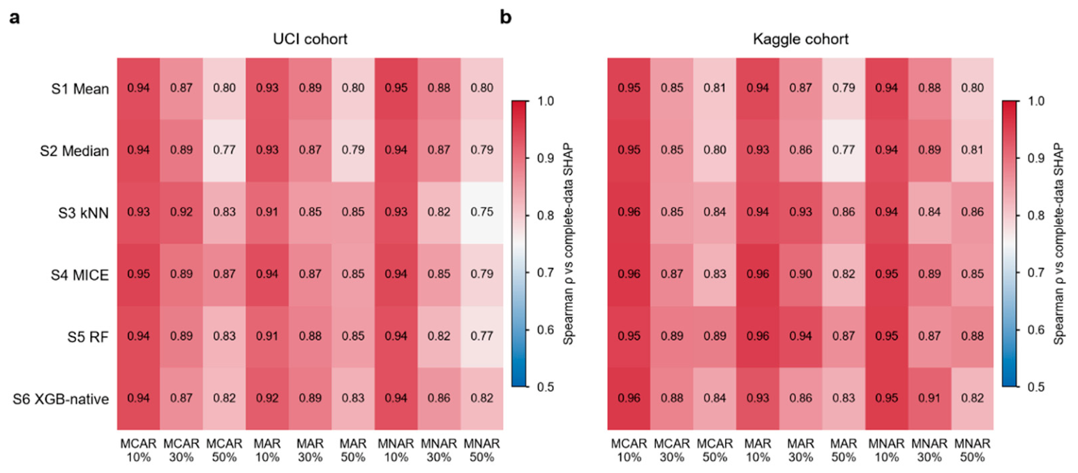
Table 1.
Imputation strategies, implementations, and hyperparameters. C1–C3 are decomposition controls and S7 a deletion reference (Section 2.4), not candidate strategies.
Table 1.
Imputation strategies, implementations, and hyperparameters. C1–C3 are decomposition controls and S7 a deletion reference (Section 2.4), not candidate strategies.
| ID | Strategy | Implementation | Key settings |
|---|---|---|---|
| S1 | Mean | SimpleImputer(strategy='mean') | Column-wise arithmetic mean of training data |
| S2 | Median | SimpleImputer(strategy='median') | Column-wise training median (robust alternative to S1) |
| S3 | k-nearest neighbours | KNNImputer | k = 5; nan-aware Euclidean distance; uniform neighbour weighting |
| S4 | MICE (multiple) | IterativeImputer + prediction-layer pooling | Bayesian-ridge chained equations; sample_posterior=True; m = 5; max_iter = 10 per imputation; imputation seeds 0–4; five independent models trained, predicted probabilities averaged |
| S5 | MissForest (single) | IterativeImputer | Random-forest backbone (30 trees); max_iter = 10; single completed dataset |
| S6 | XGBoost-native | none (L1 only) | Missing entries passed through; sparsity-aware default split direction learned per feature |
| S7 | Complete-case analysis | listwise deletion | Rows with any masked variable removed from both partitions; evaluated on complete test rows only |
| C1 | MICE single-draw control | IterativeImputer (m = 1), single model | One posterior draw, one model, isolates the value of m > 1 |
| C2 | MICE element-wise control | IterativeImputer (m = 5), pooled element-wise | Five draws averaged cell-by-cell into one completed dataset, single model, isolates the pooling layer |
| C3 | Bagged-ensemble control | SimpleImputer(strategy='mean') + 5-model bootstrap bagging | Mean imputation, five bootstrap-resampled models, predicted probabilities averaged, pure-ensemble control with no multiple imputation |
Table 2.
Downstream learner configurations, fixed across all 54 conditions.
| Hyperparameter | L1 XGBoost | L2 Logistic Regression | L3 Random Forest |
|---|---|---|---|
| Implementation | XGBClassifier | LogisticRegression | RandomForestClassifier |
| Version | 3.4.1 | scikit-learn 1.9.0 | scikit-learn 1.9.0 |
| n_estimators / max_iter | 200 | 2000 (converged) | 400 |
| max_depth | 3 | — | 8 |
| Learning rate / C | 0.1 | C = 1.0 (L2 penalty) | — |
| subsample | 0.8 | — | — |
| colsample_bytree | 0.8 | — | — |
| Regularisation | — | L2 (default) | — |
| objective / eval_metric | objective='binary:logistic' / eval_metric='logloss' | — | — |
| random_state | 0 | 42 | 42 |
| All remaining parameters | library defaults | library defaults | library defaults |
Table 4.
Three-way repeated-measures ANOVA on AUROC, by dataset and learner (subject = seed, n = 10).
Table 4.
Three-way repeated-measures ANOVA on AUROC, by dataset and learner (subject = seed, n = 10).
| Effect | UCI/L1 F (P) | UCI/L2 F (P) | UCI/L3 F (P) | Kaggle/L1 F (P) | Kaggle/L2 F (P) | Kaggle/L3 F (P) |
|---|---|---|---|---|---|---|
| Strategy | 5.96 (0.0009) | 3.30 (0.021) | 17.60 (<0.001) | 25.48 (<0.001) | 0.82 (0.520) | 25.90 (<0.001) |
| Mechanism | 0.39 (0.686) | 12.35 (0.0004) | 0.48 (0.625) | 1.21 (0.320) | 0.76 (0.483) | 0.22 (0.802) |
| Missingness rate | 22.24 (<0.001) | 45.17 (<0.001) | 87.99 (<0.001) | 19.47 (<0.001) | 6.34 (0.008) | 46.03 (<0.001) |
| Strategy × Mechanism | 2.83 (0.009) | 1.48 (0.181) | 6.11 (<0.001) | 1.81 (0.090) | 1.02 (0.430) | 1.25 (0.282) |
| Strategy × Rate | 0.81 (0.600) | 2.01 (0.058) | 1.76 (0.100) | 1.93 (0.069) | 2.03 (0.055) | 7.34 (<0.001) |
| Mechanism × Rate | 0.70 (0.600) | 4.52 (0.005) | 1.49 (0.227) | 0.99 (0.428) | 1.44 (0.241) | 2.17 (0.093) |
| S × M × R | 0.90 (0.567) | 0.74 (0.751) | 2.97 (0.0003) | 0.93 (0.541) | 0.95 (0.512) | 1.66 (0.060) |
Table 5.
Calibration metrics by strategy, L1 XGBoost, averaged across the 9 missingness conditions. E_avg is reported in Table S1 (bin-count instability at n ≈ 75).
Table 5.
Calibration metrics by strategy, L1 XGBoost, averaged across the 9 missingness conditions. E_avg is reported in Table S1 (bin-count instability at n ≈ 75).
| Strategy | UCI Brier | UCI slope | Kaggle Brier | Kaggle slope |
|---|---|---|---|---|
| S1 Mean | 0.222 ± 0.028 | 0.359 | 0.106 ± 0.011 | 0.804 |
| S2 Median | 0.220 ± 0.027 | 0.367 | 0.107 ± 0.011 | 0.801 |
| S3 kNN | 0.226 ± 0.028 | 0.327 | 0.109 ± 0.011 | 0.775 |
| S4 MICE | 0.208 ± 0.020 | 0.502 | 0.102 ± 0.011 | 0.902 |
| S5 RF | 0.229 ± 0.032 | 0.308 | 0.109 ± 0.012 | 0.779 |
| S6 XGB-native | 0.223 ± 0.028 | 0.331 | 0.107 ± 0.012 | 0.782 |
Table 7.
Minimum detectable difference (MDD) analysis by dataset and learner configuration. Each comparison is S4 versus one simpler alternative within a single missingness condition; the four-arm controls C1–C3 are analysed separately (Section 3.6) and are not part of this table. MDD = (z₀.₉₇₅ + z₀.₈₀)·s_diff/√10 (n = 10 seeds per condition; α = 0.05, two-sided; 80% power), summarised across the 9 conditions as the median and maximum MDD, alongside the largest observed absolute paired AUROC difference and the number of comparisons whose observed difference exceeded their own MDD. The MDD is descriptive and does not constitute a formal equivalence bound; no equivalence test was performed. For L1 XGBoost, S4 is compared with five alternatives (S1, S2, S3, S5 and S6), giving 5 × 9 = 45 comparisons. For L2 Logistic and L3 RF, S4 is compared with four alternatives (S1, S2, S3 and S5), giving 4 × 9 = 36 comparisons, because S6 is defined only for XGBoost. Pair-level values are provided in Table S3 (mdd_corrected.csv).
Table 7.
Minimum detectable difference (MDD) analysis by dataset and learner configuration. Each comparison is S4 versus one simpler alternative within a single missingness condition; the four-arm controls C1–C3 are analysed separately (Section 3.6) and are not part of this table. MDD = (z₀.₉₇₅ + z₀.₈₀)·s_diff/√10 (n = 10 seeds per condition; α = 0.05, two-sided; 80% power), summarised across the 9 conditions as the median and maximum MDD, alongside the largest observed absolute paired AUROC difference and the number of comparisons whose observed difference exceeded their own MDD. The MDD is descriptive and does not constitute a formal equivalence bound; no equivalence test was performed. For L1 XGBoost, S4 is compared with five alternatives (S1, S2, S3, S5 and S6), giving 5 × 9 = 45 comparisons. For L2 Logistic and L3 RF, S4 is compared with four alternatives (S1, S2, S3 and S5), giving 4 × 9 = 36 comparisons, because S6 is defined only for XGBoost. Pair-level values are provided in Table S3 (mdd_corrected.csv).
| Dataset/Learner | MDD median | MDD max | Observed max difference | Comparisons exceeding MDD |
|---|---|---|---|---|
| Kaggle/L1 XGBoost | 0.005 | 0.011 | 0.012 | 29/45 |
| Kaggle/L2 Logistic | 0.003 | 0.005 | 0.003 | 0/36 |
| Kaggle/L3 RF | 0.004 | 0.008 | 0.015 | 22/36 |
| UCI/L1 XGBoost | 0.039 | 0.061 | 0.047 | 2/45 |
| UCI/L2 Logistic | 0.025 | 0.040 | 0.020 | 1/36 |
| UCI/L3 RF | 0.033 | 0.062 | 0.091 | 8/36 |
Disclaimer/Publisher’s Note: The statements, opinions and data contained in all publications are solely those of the individual author(s) and contributor(s) and not of MDPI and/or the editor(s). MDPI and/or the editor(s) disclaim responsibility for any injury to people or property resulting from any ideas, methods, instructions or products referred to in the content. |
© 2026 by the authors. Licensee MDPI, Basel, Switzerland. This article is an open access article distributed under the terms and conditions of the Creative Commons Attribution (CC BY) license (http://creativecommons.org/licenses/by/4.0/).
Copyright: This open access article is published under a Creative Commons CC BY 4.0 license, which permit the free download, distribution, and reuse, provided that the author and preprint are cited in any reuse.