

Submitted:
20 October 2026
Posted:
21 October 2026
You are already at the latest version
Abstract
Fluid-Structure Interaction (FSI) has been the standard when simulating cerebral aneurysms. Nonetheless, obtaining a realistic aneurysm wall geometry without ex-vivo methods has proven difficult. In this article, a nodal assignment method based on empirical distributions is presented, and the effect of wall thickness is studied using one-way FSI simulations for normal and hypertensive pressure cases. Results show that while generally there is an inverse relation between structural parameters (Von-Mises stress and de-formation) and wall thickness, the final distribution of these parameters is defined by a balance between the fluid dynamics (Wall Shear Stress and hemodynamic pressure) and the thickness distribution. Comparisons between the thickness distribution and fluid dynamics were made to illustrate how these two factors affected the final structural parameter contours in the variable assignments, where hemodynamic pressure and aneurysm size were found to influence the leading factor in this duality.
Keywords:
cerebral aneurysms
; variable wall thickness
; fluid-structure interaction
1. Introduction
The study of cerebral aneurysms presents a significant clinical concern due to both their prevalence in the adult population and the potentially fatal consequences their rupture. The International Study of Unruptured Intracranial Aneurysms found that both the risk of rupture and the risk associated with surgical intervention scale strongly with aneurysm size and location, making the assessment of individual rupture risk a persistent challenge in medicine (Brisman et al., 2006; ISUIA, 1998) [1,2].
The previously mentioned line of work has linked the hemodynamic conditions inside the aneurysm sac to the biological remodeling of its wall. Regions of high and low wall shear stress (WSS) have both been associated with mechanisms of wall degeneration, growth, and rupture, suggesting that WSS distribution is not merely a fluid-dynamic parameter but an active driver of the structural weakening simulated in fluid-structure interaction (FSI) studies (Meng et al., 2014; Xiang et al., 2011) [3,4]. While there are several ways of obtaining a precise geometry for the fluid-dynamic system (the lumen) half of FSI simulations, the same cannot be said for the structural system (the arterial and aneurysm wall), so the standard has been assigning a constant wall thickness. Lately, there has been research in variable wall thickness geometry modelling.
Beyond the geometry-reconstruction methods discussed below, several studies have shown that the wall thickness assumption itself directly affects FSI results. Torii et al. (2008) [5] demonstrated that wall thickness modeling choices substantially alter the stress and deformation contours for a patient-specific aneurysm, while Voß et al. (2016) [6] directly compared constant and patient-specific wall thickness assignments and found that the resulting stress distributions differed both in magnitude and in spatial arrangement. These findings further motivate the search for wall-thickness assignment methods, such as the one presented in this article, that can approximate patient-specific variability without requiring ex-vivo proceditures.
Bolem et al. (2024) [7] presented a method of obtaining a patient-specific wall model by reconstructing 2D angiographic images into a 3D volume. Although this method produces very precise geometries, obtaining the 2D images requires surgical extraction of the aneurysm. Alagan et al. (2025) [8] made use of isosurfaces – wall thickness that decreases uniformly from the aneurysm neck – to obtain an aneurysm wall geometry without medical intervention. This method, however, does not reproduce the variability present in any given transverse section of the pathology.
Based on these two previous articles, the present study will introduce a methodology that can produce realistic aneurysm wall geometries needing only the lumen model, which can be obtained without invasive medical procedures. These wall geometries will then be coupled with the lumen model and FSI simulations will be carried out in which the effect of raising the internal pressure on the structural parameters will be studied. This methodology also builds on the previous work carried out by Díaz (2023)[9], who studied the effect of wall thickness and aneurysm size on FSI results using the same lumen geometries employed in this article, providing a baseline against which the variable-thickness assignments of this study can be compared.
2. Materials and Methods
Two base lumen geometries were selected for the FSI simulations carried out in this work, originally obtained by Valencia et al. (2006) [10] using medical images provided by the Instituto de Neurocirugía Asenjo: a lateral aneurysm located in the ICA, and a terminal aneurysm located in the MCA - both saccular and unruptured. These geometries were reconstructed from patient angiographic images and converted into STP format for meshing and simulation. Figure 1 and Figure 2 both show this reconstruction method.
The lateral geometry name implies flow runs roughly parallel to the aneurysm neck, while the terminal aneurysm sits at the artery bifurcation, where flow impinges nearly perpendicular to the neck. This distinction is expected to produce markedly different hemodynamic loading patterns between the two cases, as discussed in Section 3.1.
To correctly represent the mechanics inside both systems, the work of Amigo (2018) [11] was used extensively. In the fluid-dynamic system, user-defined functions were applied: in the inlet, a unique Womersley velocity profile was determined by Amigo for each geometry; in the outlets, an RCR Windkessel pressure condition was applied, where the constants changed depending on the pressure case (ensuring a pressure curve that varied between 120/80 mmHg for the normotensive condition and 180/100 mmHg for the hypertensive condition). The resulting pressure waveforms for both conditions are shown in Figure 3.
Finally, a non-Newtonian Casson viscosity model was applied to the blood to correctly depict the shear-thinning qualities it possesses. In the structural system, a hyperelastic deformation model was used, where the strain energy density function was constructed as a 5-parameter Mooney-Rivlin solid, whose values were determined empirically from aneurysm tissue samples in the work of Valencia et al. (2015) [12].
In FSI simulations, coupling refers to how the information between both systems is transferred. One-way coupling uses the forces the fluid exerts over the wall as initial conditions to calculate the stresses, deformations and displacements in the structural system. Two-way coupling iteratively sends back the displacements to the fluid-dynamic system to calculate how this deformation affects the flow - thus altering the forces sent to the structural system until there is convergence. Silva et al. (2023) [13] studied the effect one-way coupling has on the simulation results (compared with two-way coupling), and found that, because in one-way coupling the aneurysm wall inertia is ignored when solving the system, structural parameters like Von-Mises stress and deformation are overestimated, while fluid-dynamic parameters like streamline magnitudes and wall shear stress are underestimated. In spite of this, the structural parameter contours and patterns - areas of low and high stresses - are maintained for both types of coupling. Because of the enormous increase in computational cost that using two-way coupling entails (from 6 hours to 5 days per simulation), and given the qualitative focus of the methodology, one-way coupling was used.
The methodology presented in this article uses a nodal assignment to give thickness values to the surface of the aneurysm. The magnitude assigned is based on thickness distributions found in the literature. Kadasi et al. (2015) [14] qualitatively identified 2 main types of walls in cerebral aneurysms with diameters less than 7 [mm]: the ‘normal’ wall (NTL) and the ‘translucent’ wall (TL), the latter of which represents 33.4% of the total surface of the aneurysm and whose thickness is very reduced and uniform. Tobe et al. (2024) [15] confirmed these types of walls and quantitatively measured them to obtain the mean and standard deviation for both.
Given these distributions, each node of the outer surface of the aneurysm lumen model will be assigned a thickness value t:
where the mean and standard deviation are functions of the distance of the node with respect to the aneurysm neck z:
this ensures that the average wall thickness will decrease in the regions farther apart from the neck, as per the isosurfaces article. The constants c and k vary depending on the aneurysm model, and they are to be iteratively calibrated in such a way that the final output produces a wall geometry with an NTL average in accordance with the empirical data in Tobe’s article.
Before this assignment is made though, 1 to 10 nodes will be randomly selected as ’TL root nodes’; these TL nodes will grow to neighboring nodes - making them TL nodes too - until the ratio of TL nodes to total nodes is 33.4%, thus proportionately representing the thin-wall region. Finally, all of the TL nodes will be assigned a thickness :
where and correspond to the thin-wall distribution parameters found in Tobe’s article. To avoid lack of continuity between the aneurysm wall and the artery wall, no TL nodes were assigned for the first fifth of the total length between the neck and the aneurysm dome. The final step in the code is a Gaussian filter along the entire assignment to smooth out sharp edges, especially at the boundary between TL and NTL zones.
To develop the nodal assignment code, the LLM generative AI software Claude Sonnet 4.6 was given the requirements listed above. The MATLAB code it produced was then revised and adjustments were made to its outputs. Finally, for each lumen geometry, 4 variable wall assignments were made, and each wall-lumen model was simulated for the 2 pressure cases. On top of this, a base case with constant wall thickness assignment was carried out, for a total of 20 simulations.
After the assignment iterations the pair of constants c and k was different depending on the type of aneurysm:
Figure 4 shows that the assignment model correctly represents the decrease in thickness as the distance from the neck increases. Thin wall regions are also proportionately found in the geometry. The same behavior can be observed in the terminal geometry, where the decreasing thickness-vs-z trend and proportional TL region are obtained using the terminal-specific constants and , as shown in Figure 5.
The output that the code produces is the outer surface of the aneurysm wall. This surface was then stitched with the inner surface (the input for the code) to produce a volumetric wall geometry that shares topology with the lumen. Finally, each simulation had a 1-millisecond timestep for a total runtime of 1.75 seconds (representing 2 cardiac cycles).
3. Results
This section will be divided between the two systems involved in the simulations.
3.1. Fluid Dynamics
When comparing the hemodynamic pressure contours between the normotensive and hypertensive cases, for both geometries the case with the higher pressure has the same patterns with proportionately higher magnitudes. This is expected as the hypertensive pressure function has the same shape over time as the normotensive function, but with overall higher values and more exaggerated slopes.
However, looking at the streamlines yields a different outcome: for both pressure cases, both the shape and the magnitude of the velocity lines are the same throughout the entire geometry. This is illustrated directly by the velocity streamlines for the lateral geometry under both pressure conditions.
Figure 6 shows that no discernible difference in streamline shape or magnitude is observed between the two pressure conditions, confirming that the flow field is decoupled from the imposed outlet pressure. The same happens with the Wall Shear Stress (WSS) (shown on Figure 7), which is logical as this parameter depends entirely on the fluid velocity.
This may be counterintuitive, but it is explained by 2 facts:
- 1.
- Even though the increased pressure on the hypertensive case produces bigger deformations on the aneurysm wall (shown in Figure 13), because of the one-way coupling made, this extra deformation is not communicated back to the fluid-dynamic system, thus not altering the streamlines.
- 2.
- The velocity inlet boundary condition imposes a velocity magnitude on every timestep. This means that, when the pressure is raised in the outlets, to maintain the velocity condition the inlet pressure is raised proportionately - this means even though the pressure is higher, the pressure difference is the same in both cases.
As a consequence of these two conditions, the blood flow is independent from the hemodynamic pressure. This makes sense physiologically, as hypertension does not cause the blood to change velocity, but rather it makes the heart work harder to pump this blood. Comparing the pressure distribution between the two aneurysm types reveals a further pattern related to their anatomical orientation.
Figure 8 shows that while the lateral geometry shows a more diffuse pressure gradient in the aneurysm (consistent with parallel flow past the neck), the terminal geometry shows a localized high-pressure region where the bifurcating flow impinges directly on the dome. When integrating this parameter over the aneurysm surface during systole, the hemodynamic pressure was 19.4% and 14.0% higher in the terminal geometry than in the lateral geometry, for the normotensive and hypertensive cases respectively. A similar geometry-dependent effect is observed for the WSS: averaged over the aneurysm sac in the systole, WSS for the terminal geometry was 2.13 times higher than in the lateral geometry, consistent with the flow impinging directly on the wall at the bifurcation rather than running tangentially along it.
3.2. Structural System
The analysis done in this article mainly compares the effect of wall thickness vs. the effect of the fluid dynamics on the final distributions of structural parameters - Von-Mises stress and deformation. The role of fluid dynamics is hard to quantify because this term applies to both WSS and hemodynamic pressure, so to standardize the comparisons, the simulations without the variable assignment method will be used as qualitative references: because in these cases the thickness is constant, this parameter does not influence the final contours of Von-Mises stress or deformation - only its magnitude.
Then, the distribution of Von-Mises stress on the constant assignments will be dubbed ’fluid-dynamic stresses’ to compare with the Von-Mises stress distribution on the variable assignments. Figure 9 illustrates how both parameters influence the final fluid-dynamic stress distribution.
For the variable assignments, 3 points of interest will be defined for analysis:
- Point 1 corresponds to the place in the external surface of the aneurysm wall where the Von-Mises stress is maximum.
- Point 2 corresponds to the place in the external surface of the aneurysm wall where the thickness is minimal.
Figure 10 shows these 3 points imposed over both the thickness map and the Von-Mises stress distribution of terminal assignment 3.
It is logical to assume that the location of Point 1 and Point 2 would be the same, as an inverse relation between wall thickness and Von-Mises stress has been found extensively in the literature. This does occur on lateral assignment number 3 and terminal assignments numbers 2 & 4, and it is because in these assignments Point 2 is located on an area where the fluid-dynamic stresses are high, so the combination of this plus the low thickness multiplies the final Von-Mises stresses on this point, resulting in a concordant Point 1 and Point 2.
Figure 11 illustrates this phenomenon: Point 2 is located on a zone where the fluid-dynamic stresses are elevated. Even though the maximum fluid-dynamic stress is not exactly where Point 2 is, the final Von-Mises stress distribution is displaced around the point of minimum thickness. This did not occur on the majority of the simulations however; in most cases Point 1 and Point 2 were on different places.
This happens when the place of minimum thickness is located in an area where the fluid-dynamic stresses are low, so the ’multiplier’ effect described in the previous case does not occur. Instead, Point 1 will be located in a zone where there is a balance of high-enough fluid-dynamic stress and low-enough thickness. Figure 12 illustrates this point; when overlaying Point 1’s location on the fluid-dynamic stress distribution, one can see that to the top of this location the stresses are higher; however, the thickness is higher as well, so this maximum Von-Mises stress corresponds to that where the combination of that particular thickness with that particular fluid-dynamic stress yielded the highest magnitude.
In addition to the notable points analysis made, a more direct comparison between wall thickness and structural parameters was carried out by measuring on a cross section between the aneurysm neck and Point 1 how the reduction in thickness affected both Von-Mises stress and deformation on the wall.
Figure 13 shows that both deformation and Von-Mises stress rise when wall thickness decreases, with the slope of the curve increasing asymptotically as thickness goes to 0. The difference between pressure cases can also be appreciated in the graph, where for both parameters the shape of the curve is preserved, but the magnitudes rise, which makes sense because the hypertensive pressure curve also preserves the same temporal shape as the normotensive one, with higher magnitudes.
Results show that both fluid dynamics and wall thickness play an important role in the final stress and deformation distributions in the aneurysm wall. In an attempt to compare the influence of these two factors, a comparison was made between the Von-Mises stress and deformation present at Point 3 of the variable assignments versus the same parameters on Point 1 of the constant assignment. Because the constant assignment distribution was defined previously as the fluid-dynamics stress, Point 1 represents the area on the respective geometry where the fluid dynamics have maximum influence, so comparing it to a point with lower wall thickness (and moderate structural parameters) can serve to paint a picture of the relation of the thickness/fluid dynamics duality described.
Figure 14 illustrates this comparison. The left aneurysm shows the point with lower wall thickness, but also lower fluid-dynamic stresses, while the right aneurysm shows the point with higher wall thickness but higher fluid-dynamic stresses. The average stress and deformation on the thickness points were compared against the parameters on the fluid-dynamic point:
Table 1 shows that the points with a greater influence of fluid dynamics yielded higher stresses than the point of lower thickness on the lateral geometry, while the opposite happens on the terminal geometry. This can be explained by the effect of the aneurysm size, as the terminal geometry is much smaller than its lateral counterpart (which has double the aneurysm diameter), so the stress magnitude on the wall is also smaller, as per Laplace’s Law. Because of these lower magnitudes, wall thickness appears to have more influence than fluid dynamics on the final stress distribution, and the opposite occurs on the higher-magnitude lateral geometry. This relation between the two points is maintained in the hypertensive pressure case, but the percentage increase is reduced.
Every variable assignment produces higher average stress and deformation than its respective constant-thickness case, and the lateral geometry consistently yields higher magnitudes than the terminal geometry across all assignments and pressure conditions.
4. Discussion
The methodology presented in this article was successful in producing an aneurysm wall geometry that correctly depicted the variation in thickness found in real samples, proportionately placing both types of wall in the final configuration and representing the decrease in its thickness when the distance to the aneurysm neck increased. This result could be achieved without invasive medical procedures.
Results of simulating the wall dynamics showed that there is an inverse relation between structural parameters and wall thickness, with the thin-wall regions presenting much larger Von-Mises stresses and deformation than the normal wall. Nonetheless, the distributions also showed that fluid dynamics is a factor that cannot be ignored when evaluating this relationship, as the points of maximum structural parameters were determined by a combination between wall thickness and fluid dynamics. To evaluate the latter, the constant assignment was used, as the wall thickness has no influence on the final contours of the stress distributions, only changing its magnitudes. The ’fluid-dynamic stresses’, as this distribution was dubbed, were found to be a very useful qualitative tool to evaluate how the fluid-dynamic domain affects its structural counterpart.
These findings are consistent with a broader effect of aneurysm type on the structural results. Despite the terminal geometry presenting higher average hemodynamic pressure and WSS (Section 3.1), its average Von-Mises stress and deformation were consistently lower than the lateral geometry’s — 36% and 48% lower for stress, and 24% and 27% lower for deformation, in the normotensive and hypertensive cases respectively. This apparent contradiction was resolved by the strong dependence of wall stress on aneurysm size: the lateral aneurysm has roughly 3.93 times the surface area, 7.7 times the volume, and twice the diameter of the terminal aneurysm, so that despite its comparatively milder hemodynamic loading, its larger radius dominates the resulting wall stress, following Laplace’s Law for thin-walled pressure vessels.
As the final structural parameters distribution in the aneurysm wall was affected by both wall thickness and fluid-dynamic stresses, the comparison shown in Figure 14 was an attempt to paint a picture of how the influence of these factors changed. The results illustrated that the balance between this influence depended on hemodynamic pressure and aneurysm size, but most certainly these are not the only parameters that matter, as aspect ratio, vorticity, aneurysm location relative to inlets and outlets, among others, also must determine the final contours, so further analysis using the aneurysm wall assignment must take those factors into consideration.
Even though the methodology was successful, the biggest limitation of the simulations carried out was the use of one-way coupling, as it introduced magnitude errors in the stress and deformation distributions. The full scope of the effect this had can be easily studied, as the MATLAB code provides a seed for each wall assignment, so simulations using the same geometry and boundary conditions but two-way coupling can be set up.
The implementation of the thin-wall regions in the code proved successful at representing the uniformity of its thickness, as the growth algorithm ensures the area of the TL zone is large enough to not get diffused by the final Gaussian filter. A possible improvement for future work is to forgo the random assignment of initial TL root nodes, instead taking into consideration the Wall Shear Stress distribution of the fluid-dynamic system, as the thin-wall region is formed in areas where tissue wear is high, so this parameter paints an accurate picture of where this type of wall will form, so modifying the code and making high WSS points more likely to be TL root nodes is the logical step forward.
Finally, the evolution shown in Figure 13 accurately represented the increase in structural parameters as wall thickness decreased, as well as the preservation of the shape of this function but an increase in its magnitude in the hypertensive pressure case. A weak point of this analysis was that the method used to take the measurements depends heavily on fluid-dynamics, as the cross section chosen is arbitrary. To account for this in future work, a nodal analysis is recommended, where wall thickness, Von-Mises stress and deformation are measured for every node in the geometry, so the resulting graph is a scatter plot where even though the general shape of the curve will be the same as the one presented in this article, multiple values of structural parameters will exist for the same wall thickness, thus representing the influence of fluid-dynamics.
5. Conclusions
The methodology presented in this article succeeded at producing realistic aneurysm wall geometries from the lumen model alone, thus avoiding invasive procedures. This allowed the thickness distribution to be directly related to the contours of Von-Mises stress and deformation: in general, the thin-wall regions showed much larger structural parameters. This inverse relation was preserved, with higher magnitudes, in the hypertensive case.
However, the location of the maximum structural parameters was not defined by thickness alone. The final contours resulted from a balance between the thickness distribution and the fluid-dynamic loading. The influence of each factor was studied, with hemodynamic pressure and aneurysm size playing a role in altering this balance. Because of this, wall thickness cannot be studied in isolation, and the role of fluid dynamics must be considered when interpreting any thickness-stress relationship.
Future work should study this duality in greater depth. To do so, it is recommended to use two-way coupling to remove the magnitude errors of the one-way approach and to remove the independence of fluid dynamics from the structural system, to edit the assignment code to link the placement of thin-wall regions to the Wall Shear Stress distribution, and to carry out a nodal analysis of thickness and structural parameters. Additional factors such as aspect ratio, vorticity and aneurysm location relative to the inlets and outlets should also be considered.
Funding
This research received no external funding.
Data Availability Statement
For the variable wall assignment code, the simulations carried out, or other data, feel free to contact the authors of this article at the e-mails provided above.
Conflicts of Interest
The authors declare no conflicts of interest.
Abbreviations
The following abbreviations are used in this manuscript:
| FSI | Fluid Structure Interaction |
| TL | Translucent wall |
| NTL | Not translucent wall |
| WSS | Wall Shear Stress |
References
- Brisman, J. L.; Song, J. K.; Newell, D. W. Cerebral aneurysms. N. Engl. J. Med. 2006, 355(9), 928–939. [Google Scholar] [CrossRef] [PubMed]
- International Study of Unruptured Intracranial Aneurysms Investigators. Unruptured intracranial aneurysms—risk of rupture and risks of surgical intervention. N. Engl. J. Med. 1998, 339(24), 1725–1733. [PubMed]
- Meng, H.; Tutino, V. M.; Xiang, J.; Siddiqui, A. High WSS or low WSS? Complex interactions of hemodynamics with intracranial aneurysm initiation, growth, and rupture: toward a unifying hypothesis. Am. J. Neuroradiol. 2014, 35(7), 1254–1262. [Google Scholar] [CrossRef] [PubMed]
- Xiang, J.; Natarajan, S. K.; Tremmel, M.; Ma, D.; Mocco, J.; Hopkins, L. N.; et al. Hemodynamic–morphologic discriminants for intracranial aneurysm rupture. Stroke 2011, 42(1), 144–152. [Google Scholar] [CrossRef] [PubMed]
- Torii, R.; Oshima, M.; Kobayashi, T.; et al. Fluid–structure interaction modeling of a patient-specific cerebral aneurysm: influence of structural modeling. Comput Mech. 2008, 43, 151–159. [Google Scholar] [CrossRef]
- Voß, S.; Glaßer, S.; Hoffmann, T.; Beuing, O.; Weigand, S.; Jachau, K.; et al. Fluid-structure simulations of a ruptured intracranial aneurysm: Constant versus patient-specific wall thickness. Comput. Math. Methods Med. 2016, 2016(1), 9854539. [Google Scholar] [CrossRef] [PubMed]
- Bolem, S.; Valeti, C.; Philip, N. T.; Sudhir, B. J.; Patnaik, B. S. V. Patient-specific arterial wall generation for intracranial aneurysms with a variable and a near realistic vessel wall thickness for FSI studies. Med. Eng. Phys. 2024, 130, 104211. [Google Scholar] [CrossRef] [PubMed]
- Alagan, A. K.; Valeti, C.; Bolem, S.; Karve, O. S.; Arvind, K. R.; Rajalakshmi, P.; et al. Histopathology-based near-realistic arterial wall reconstruction of a patient-specific cerebral aneurysm for fluid-structure interaction studies. Comput. Biol. Med. 2025, 185, 109579. [Google Scholar] [CrossRef] [PubMed]
- Díaz, D.; Valencia, Á. Study of the effects of wall thickness and size variations on the rupture risk of cerebral aneurysms using FSI simulations. Appl. Sci. 2024, 14(15), 6717. [Google Scholar] [CrossRef]
- Valencia, Á.; Zárate, A.; Gálvez, M.; Badilla, L. Non-Newtonian blood flow dynamics in a right internal carotid artery with a saccular aneurysm. Int. J. Numer. Meth. Fluids 2006, 50, 751–764. [Google Scholar] [CrossRef]
- Amigo, N.; Valencia, Á. Determining significant morphological and hemodynamic parameters to assess the rupture risk of cerebral aneurysms. J. Med. Biol. Eng. 2019, 39(3), 329–335. [Google Scholar] [CrossRef]
- Valencia, A.; Contente, A.; Ignat, M.; Mura, J.; Bravo, E.; Rivera, R.; Sordo, J. Mechanical test of human cerebral aneurysm specimens obtained from surgical clipping. J. Mech. Med. Biol. 2015, 15(05), 1550075. [Google Scholar] [CrossRef]
- Silva, M. L. F. D.; Goncalves, S. D. F.; Haniel, J.; Lucas, T. C.; Huebner, R. Comparative study between 1-way and 2-way coupled fluid-structure interaction in numerical simulation of aortic arch aneurysms. An. Da Acad. Bras. De Ciências 2023, 95, e20210859. [Google Scholar] [CrossRef] [PubMed]
- Kadasi, L. M.; Dent, W. C.; Malek, A. M. Cerebral aneurysm wall thickness analysis using intraoperative microscopy: effect of size and gender on thin translucent regions. J. Neurointerventional Surg. 2013, 5(3), 201–206. [Google Scholar] [CrossRef] [PubMed]
- Tobe, Y.; Yagi, T.; Kawamura, K.; Suto, K.; Sawada, Y.; Hayashi, Y.; et al. Three-dimensional wall-thickness distributions of unruptured intracranial aneurysms characterized by micro-computed tomography. Biomech. Model. Mechanobiol. 2024, 23(4), 1229–1240. [Google Scholar] [CrossRef] [PubMed]
Figure 1.
Angiography (left) and STP geometry (right) for the lateral aneurysm.
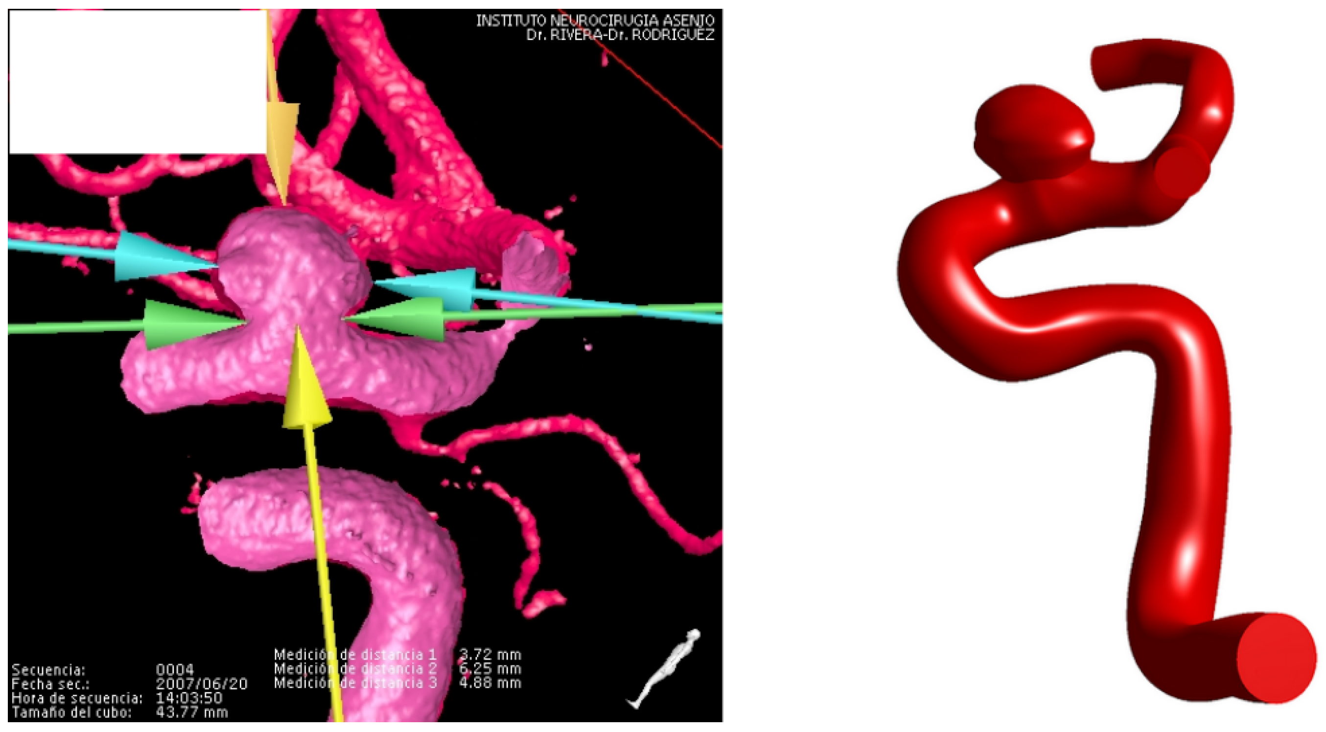
Figure 2.
Angiography (left) and STP geometry (right) for the terminal aneurysm.
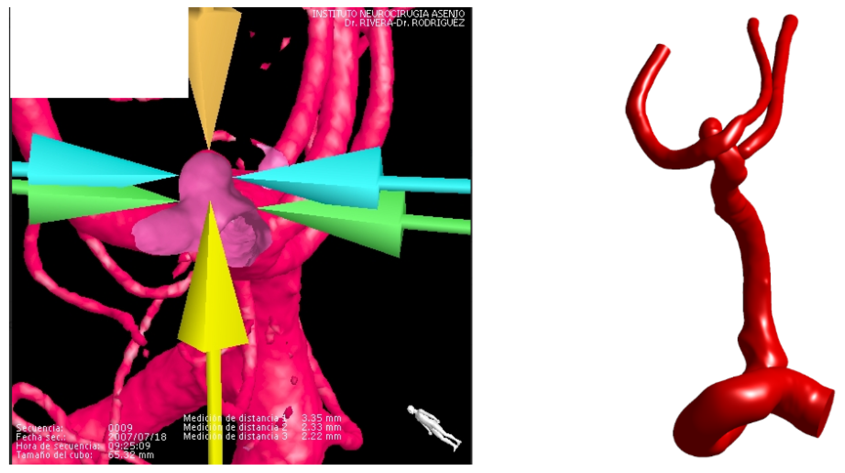
Figure 3.
Pressure curves for both cases.
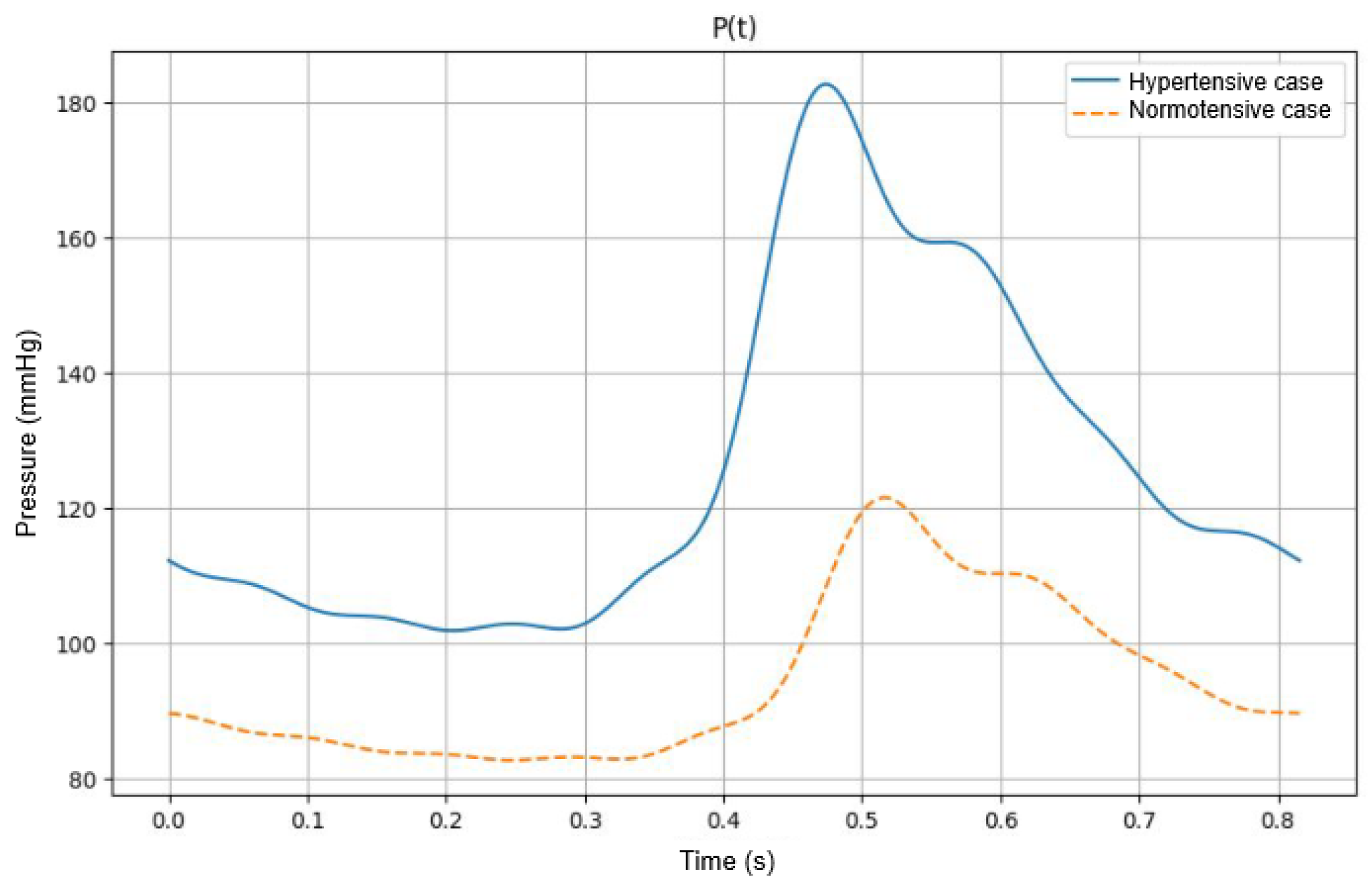
Figure 4.
Thickness map and nodal thickness graph for lateral assignment number 2.
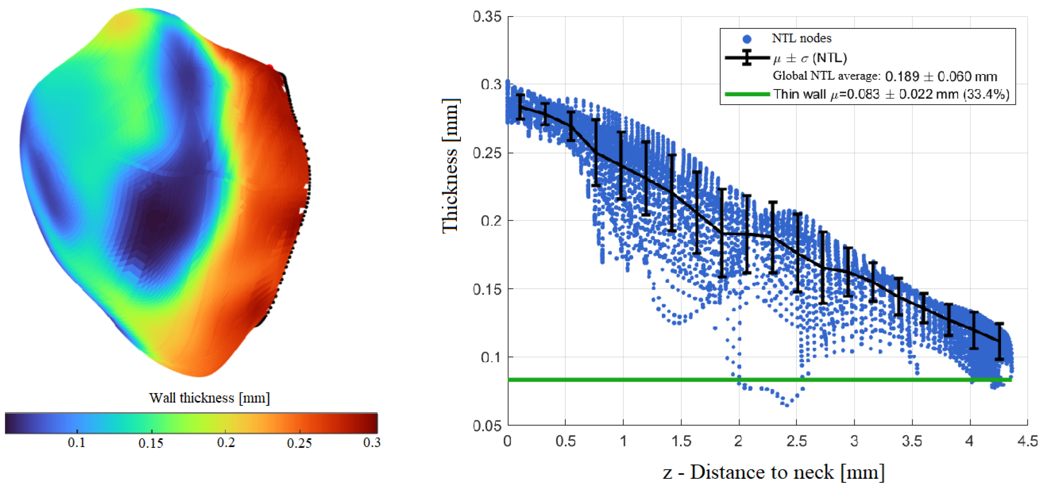
Figure 5.
Thickness map and nodal thickness graph for terminal assignment number 4.
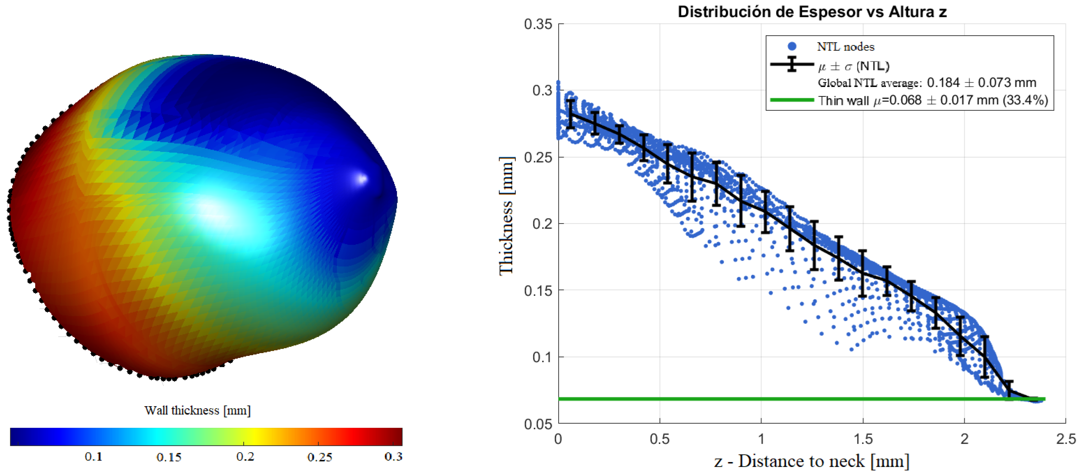
Figure 6.
Systolic velocity streamlines in the lateral geometry for both pressure cases.
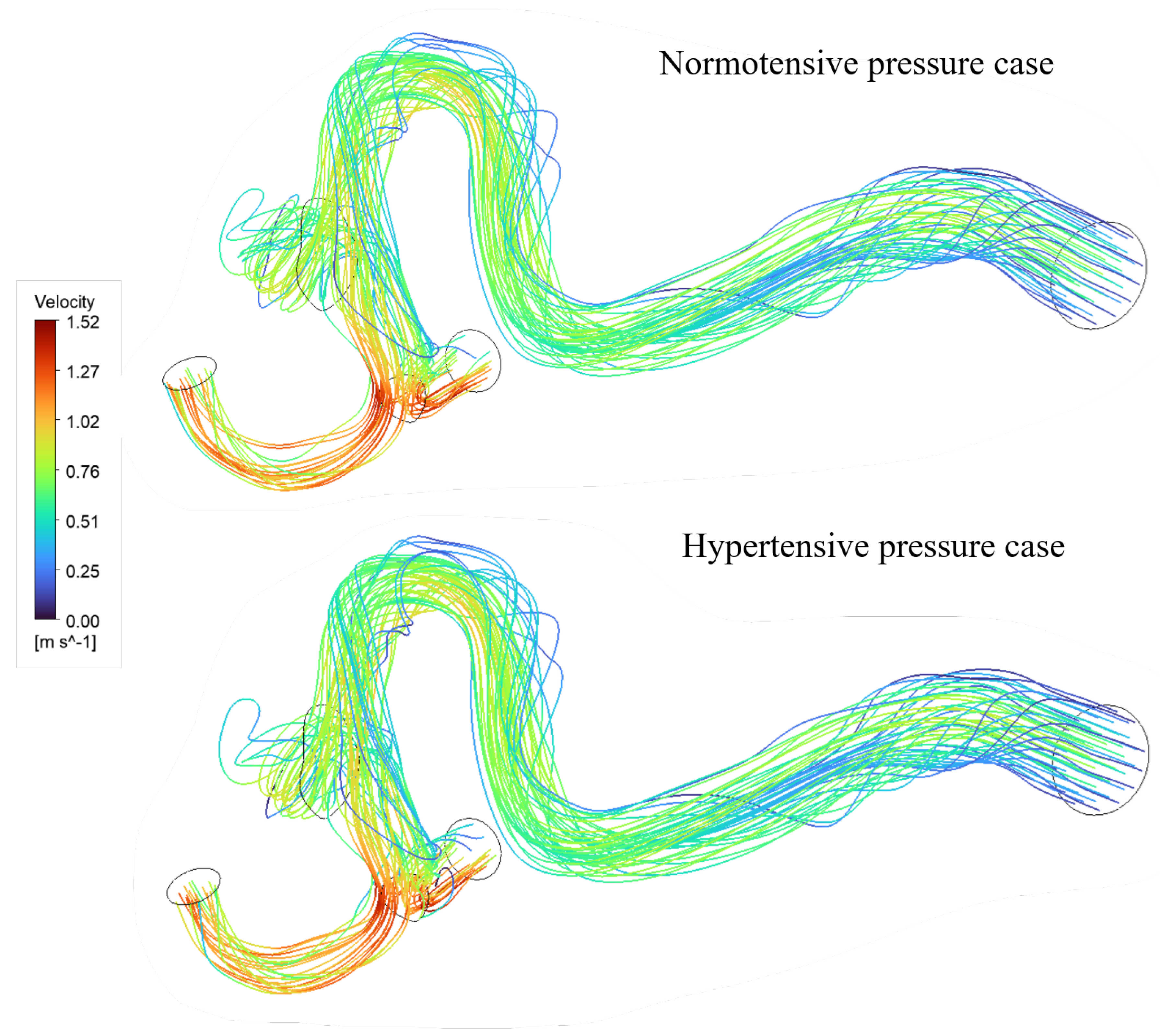
Figure 7.
Wall Shear stress contours for the lateral geometry in both pressure cases.
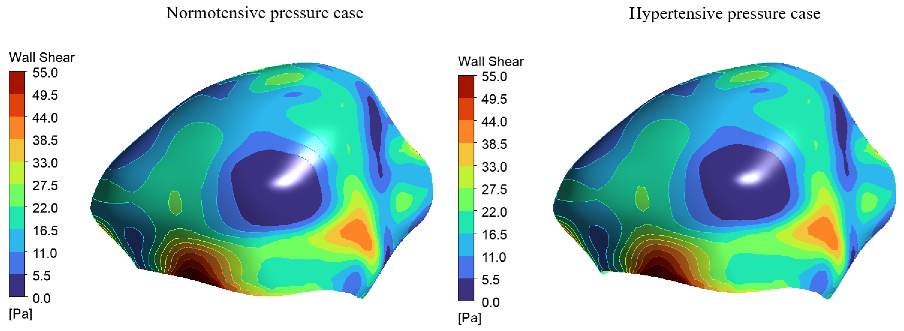
Figure 8.
Normotensive systolic pressure distributions for both geometries.
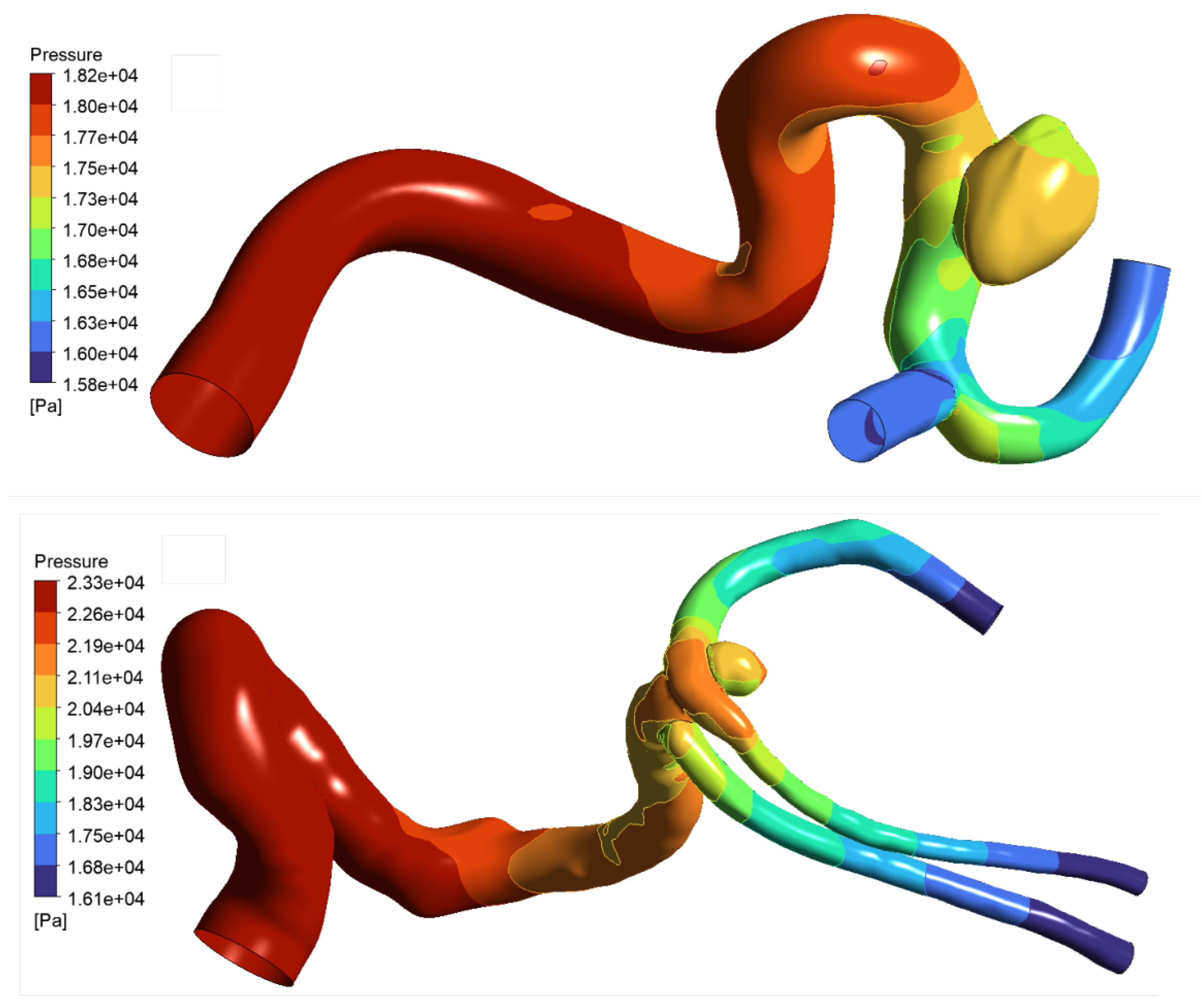
Figure 9.
WSS and pressure contours for the constant lateral assignment and how they contribute to the final Von-Mises stress distribution.
Figure 9.
WSS and pressure contours for the constant lateral assignment and how they contribute to the final Von-Mises stress distribution.
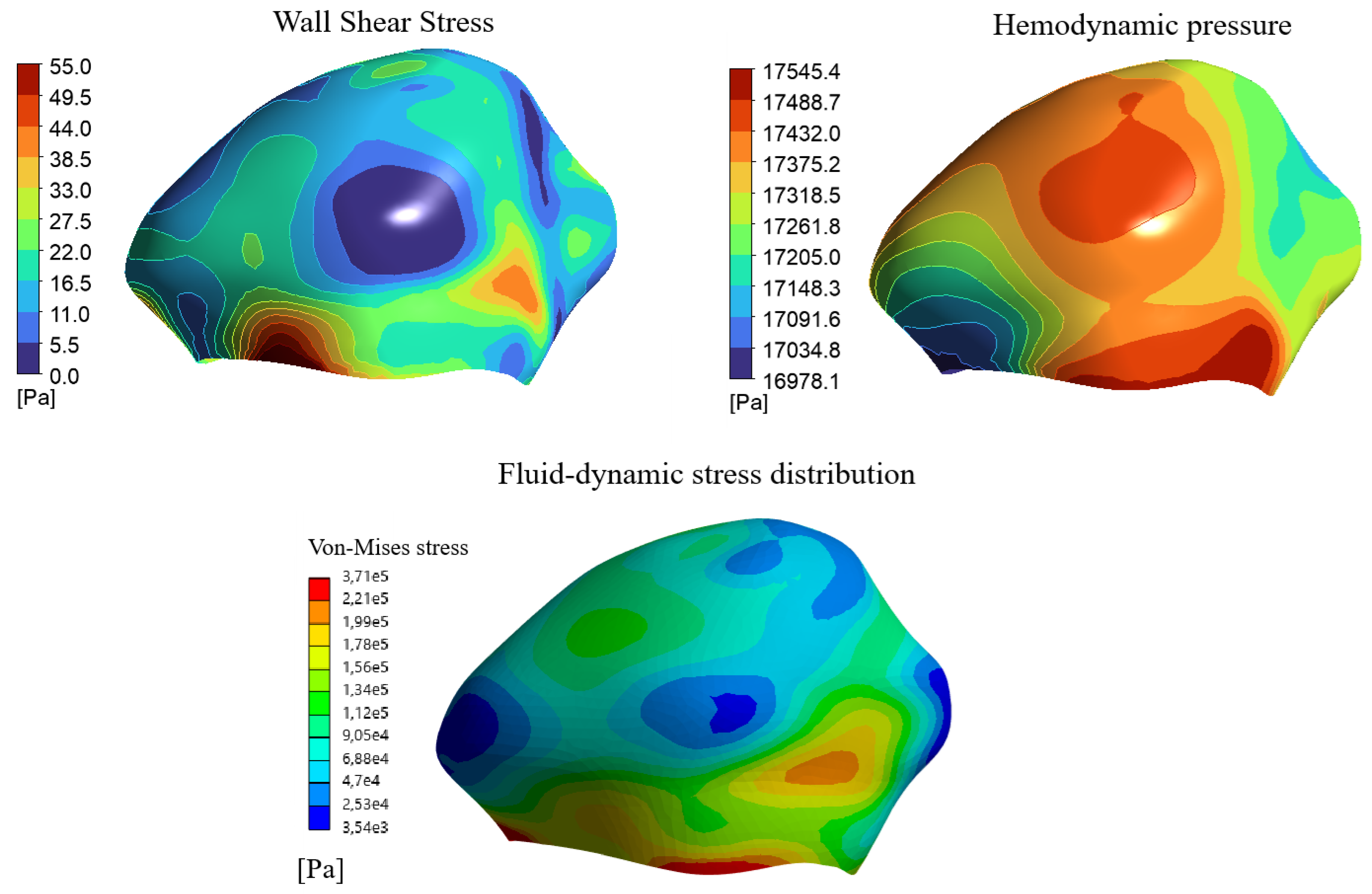
Figure 10.
The points of interest mapped on terminal assignment number 3.
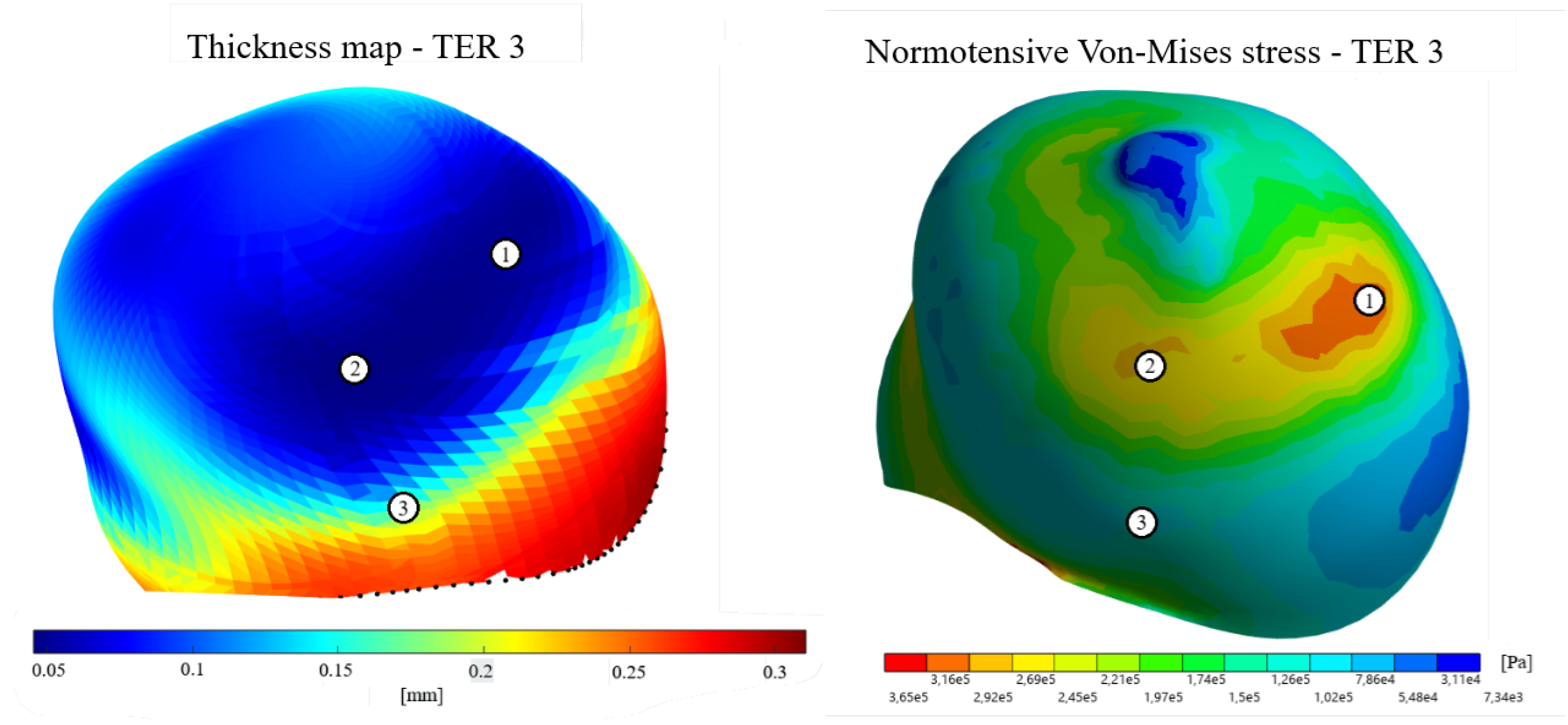
Figure 11.
Influence of wall thickness and fluid-dynamic stresses on the final Von-Mises stress distribution on lateral assignment number 3.
Figure 11.
Influence of wall thickness and fluid-dynamic stresses on the final Von-Mises stress distribution on lateral assignment number 3.
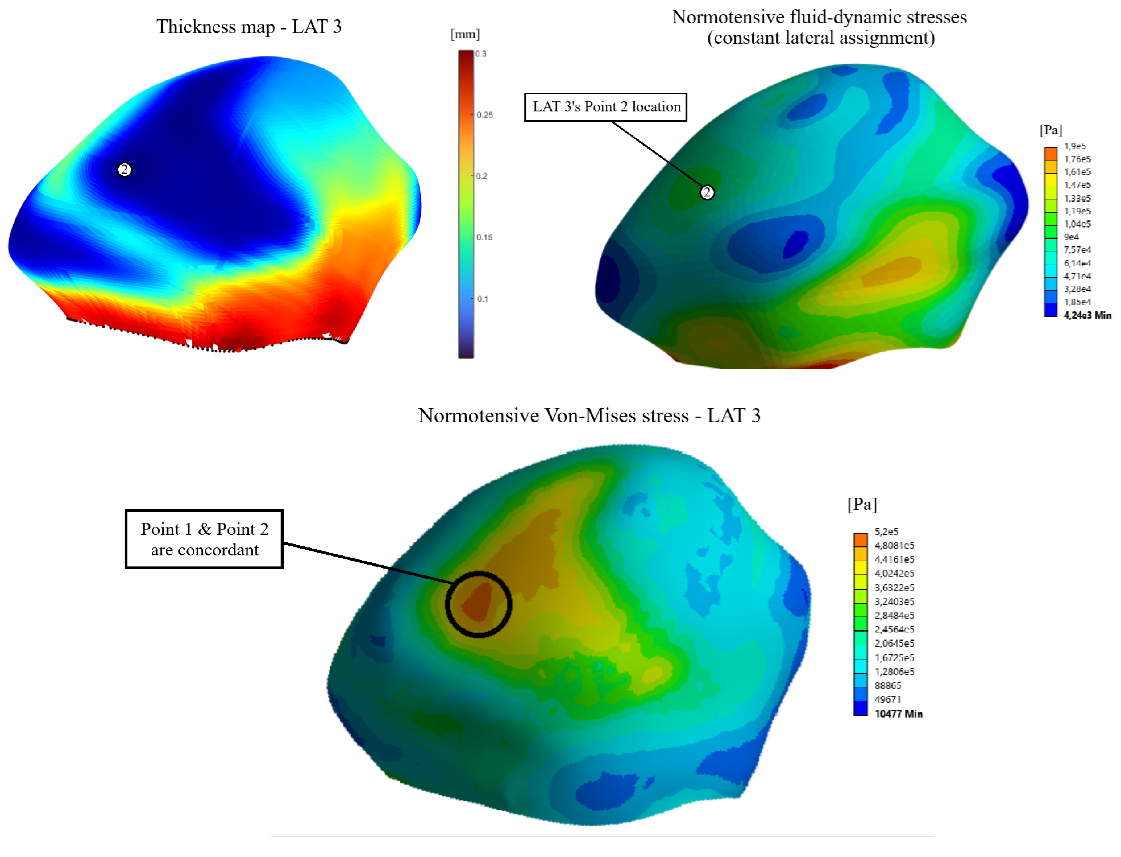
Figure 12.
Influence of wall thickness and fluid-dynamic stresses on the final Von-Mises stress distribution on terminal assignment number 1.
Figure 12.
Influence of wall thickness and fluid-dynamic stresses on the final Von-Mises stress distribution on terminal assignment number 1.
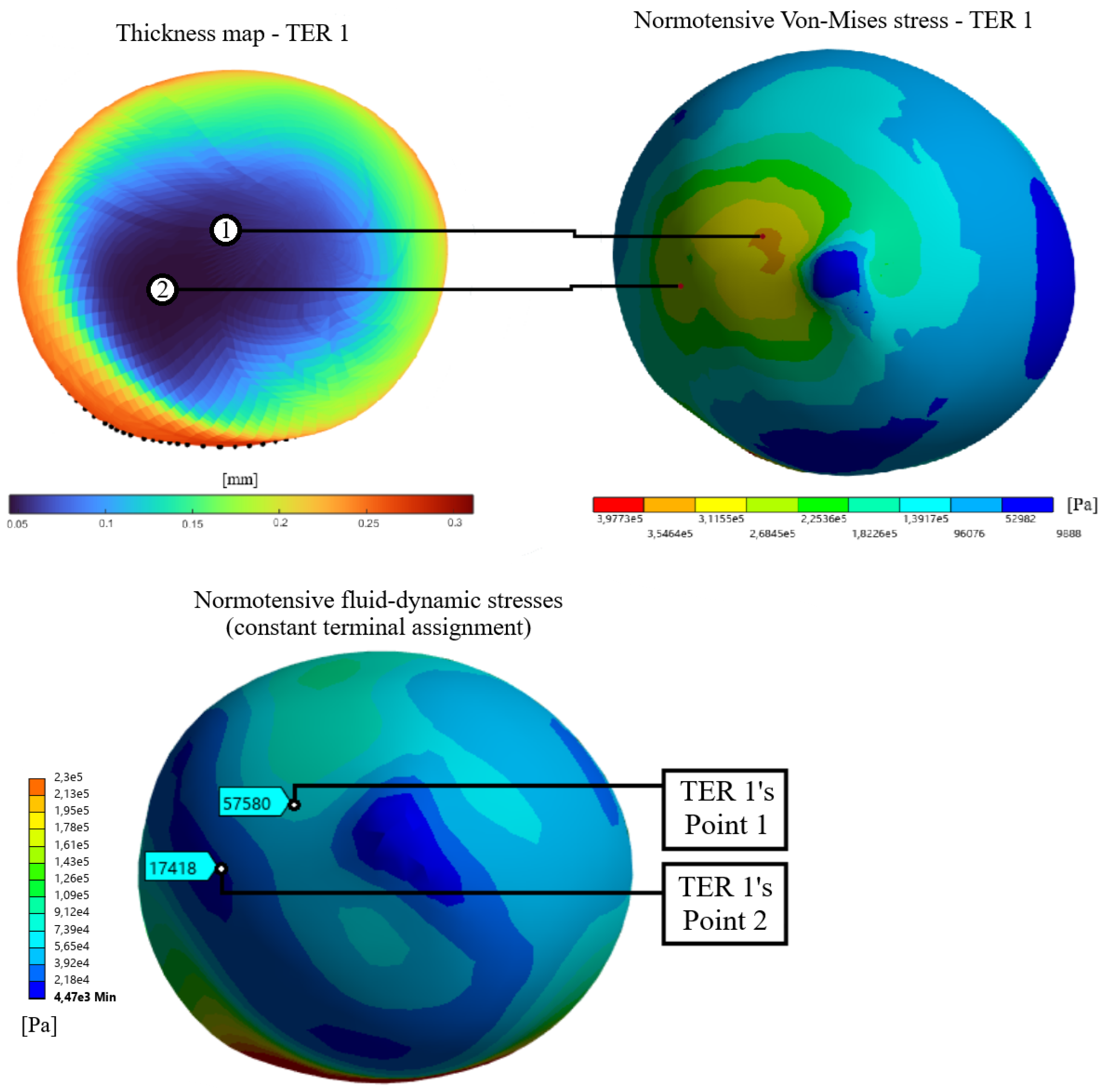
Figure 13.
Cross section along the aneurysm wall where measurements were made to make the graphs of structural parameters as functions of wall thickness.
Figure 13.
Cross section along the aneurysm wall where measurements were made to make the graphs of structural parameters as functions of wall thickness.
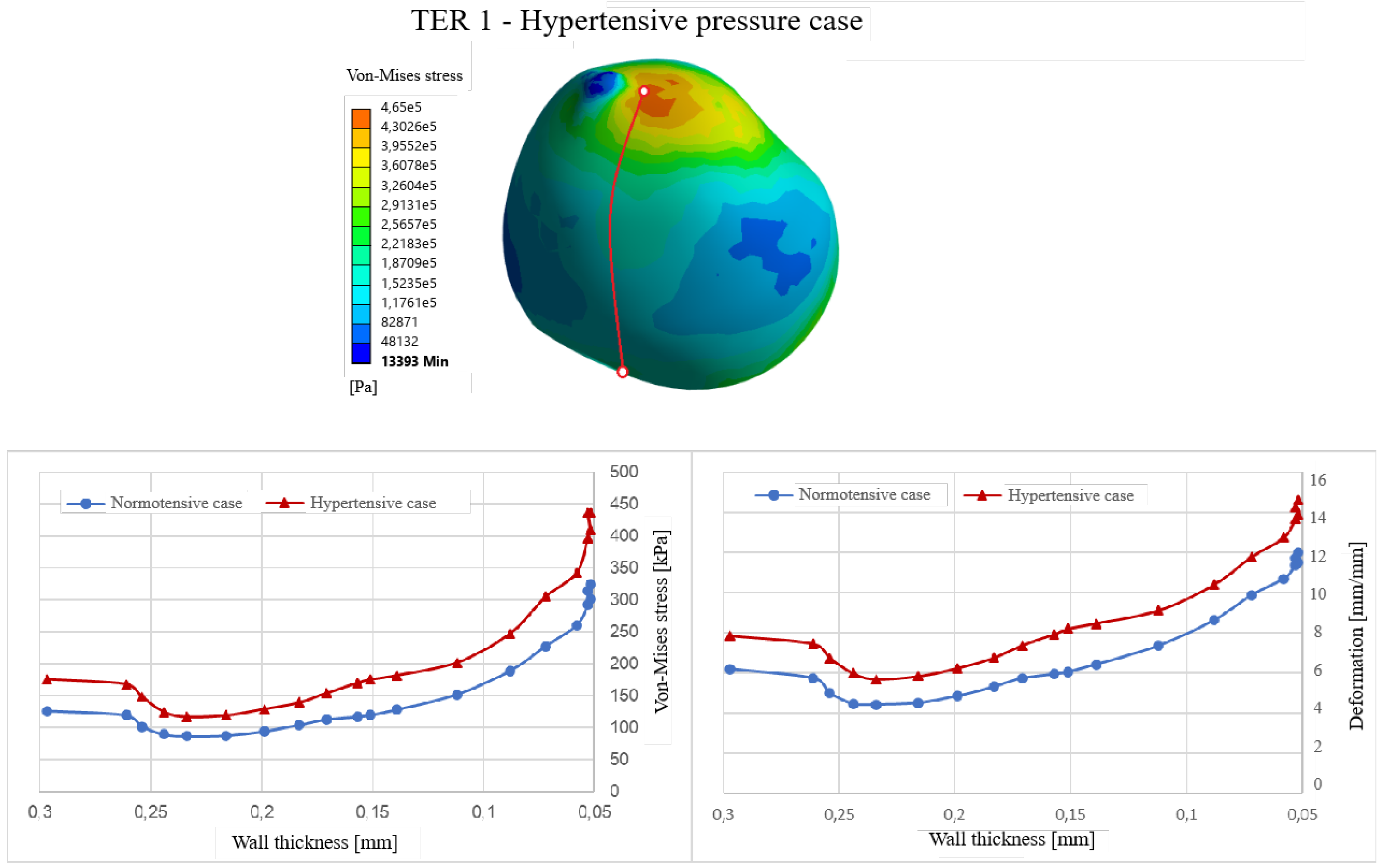
Figure 14.
Points compared in the duality analysis.
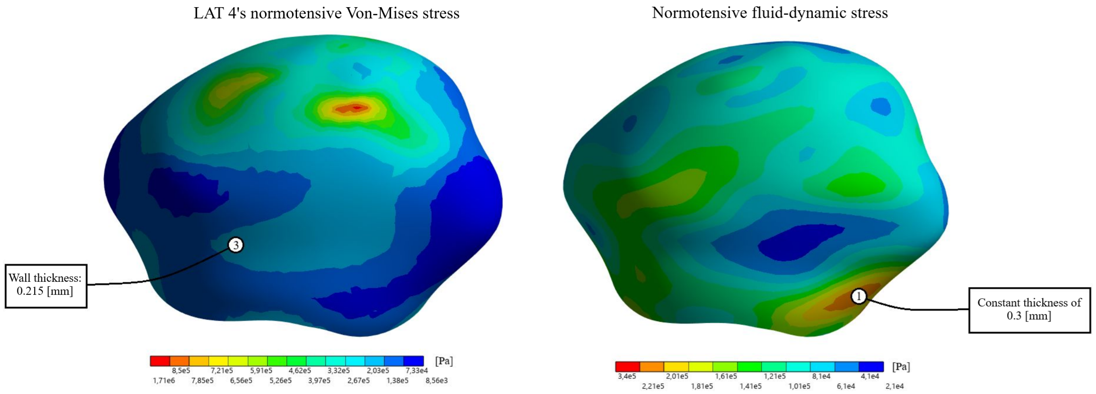

Table 1.
Decrease/Increase in structural parameters between the thickness point and the fluid-dynamic point.
Table 1.
Decrease/Increase in structural parameters between the thickness point and the fluid-dynamic point.
| Geometry | V-M Stress (Norm.) | V-M Stress (Hyp.) | Deformation (Norm.) | Deformation (Hyp.) |
|---|---|---|---|---|
| Lateral | -20.2% | -9.5% | -17.3% | -7.0% |
| Terminal | +26.4% | +23.8% | +21.3% | +17.2% |
Table 2.
Average Von-Mises stress and deformation for the lateral assignments.
| Assignment | V-M Stress (Norm.) [kPa] | V-M Stress (Hyp.) [kPa] | Deformation (Norm.) [%] | Deformation (Hyp.) [%] |
|---|---|---|---|---|
| Constant LAT | 96.93 | 145.91 | 4.72 | 6.60 |
| LAT 1 | 214.10 | 328.79 | 8.42 | 11.09 |
| LAT 2 | 204.08 | 312.85 | 8.23 | 10.87 |
| LAT 3 | 204.58 | 333.78 | 8.41 | 11.14 |
| LAT 4 | 185.40 | 284.50 | 7.60 | 10.12 |
Table 3.
Average Von-Mises stress and deformation for the terminal assignments.
| Assignment | V-M Stress (Norm.) [kPa] | V-M Stress (Hyp.) [kPa] | Deformation (Norm.) [%] | Deformation (Hyp.) [%] |
|---|---|---|---|---|
| Constant TER | 74.53 | 106.35 | 3.73 | 5.06 |
| TER 1 | 144.91 | 208.70 | 6.59 | 8.61 |
| TER 2 | 151.63 | 216.58 | 6.72 | 8.67 |
| TER 3 | 126.00 | 181.90 | 5.90 | 7.78 |
| TER 4 | 169.04 | 239.16 | 7.19 | 9.14 |
Disclaimer/Publisher’s Note: The statements, opinions and data contained in all publications are solely those of the individual author(s) and contributor(s) and not of MDPI and/or the editor(s). MDPI and/or the editor(s) disclaim responsibility for any injury to people or property resulting from any ideas, methods, instructions or products referred to in the content. |
© 2026 by the authors. Licensee MDPI, Basel, Switzerland. This article is an open access article distributed under the terms and conditions of the Creative Commons Attribution (CC BY) license (http://creativecommons.org/licenses/by/4.0/).
Copyright: This open access article is published under a Creative Commons CC BY 4.0 license, which permit the free download, distribution, and reuse, provided that the author and preprint are cited in any reuse.