

Submitted:
16 October 2026
Posted:
20 October 2026
You are already at the latest version
Abstract
Does access to transaction-level records affect which forecasting method public-finance analysts should choose? To answer this question, we compare four forecasting strategies applied to a short, highly seasonal time series of child-benefit payments: top-down, bottom-up, data-enrichment, and minimum-trace reconciliation. Our application concerns monthly child-benefit expenditure in Republika Srpska (Bosnia and Herzegovina), where we have approximately a hundred observations of total payments, but more than a million observations of individual payments. We also consider four different ways to deal with the recurring near-zero observations typical of administrative payment data. Under an expanding-window design, where each model can only use information available at the time of each forecast origin, exponential smoothing performs best across every treatment, with minimum-trace reconciliation yielding statistically equivalent accuracy. Enrichment with features from microdata offers no advantage when those features must be known in advance, while machine-learning techniques fail to outperform the benchmarks. The choice of treatment for near-zero observations proves as important as the forecasting method itself. Overall, in the presence of strong seasonality and short time-series, widely-used forecasting techniques remain hard to improve upon, and more data only helps if it provides genuinely forward-looking information.
Keywords:
benchmark forecasting
; exponential smoothing
; forecast reconciliation
; machine learning
; social protection expenditure
1. Introduction
Social protection agencies, fiscal authorities, statistical offices and, generally, governments, must forecast (benefit) expenditure months or even years ahead to support budget allocation, risk and actuarial assessments, along with policy evaluation. The methods to perform such tasks are numerous and have been researched to a greater extent over this and the past century, as a systematic review of four decades of budget-forecasting research documents [1]. Child benefit programmes may be somewhat a representative case for several reasons which can be contracted into the following. First, payments are numerous, individually quite small and are governed by legislated eligibility rules. Moreover, they are periodically reindexed by policy decision, which results in the fact that the aggregate expenditure series, in the end, combine demographic dynamics with policy induced level shifts. In Republika Srpska (Bosnia and Herzegovina), child benefits are administered through the Public Child Protection Fund and indexed annually to the minimum wage [2,3,4]. This way, an aggregate series is produced that is short in the statistical sense, a little over a hundred monthly observations in the frame this paper shall deal with. However, these observations are underpinned by more than a million individual payment records. This combination of a short target series and rich administrative microdata is common in the public sector and raises a practical question that this paper tries to address directly: Does the availability of transaction-level microdata change which forecasting method a public-finance statistician should use?
The natural reference points for such a question are usually the benchmark forecasting models. These models usually include but are not limited to: the seasonal naive method, ETS model, seasonal ARIMA with or without exogenous drivers, and the Theta method [5]. Decades of empirical evidence, most prominently from the M-competition series [6,7,8], show that these simple and transparent models are more often than not difficult to beat, and that individually trained machine learning (ML) models frequently underperform them on short series [9], in spite of different other findings [10,11] as well. The M4 competition, however, also showed that ML can become competitive when it is hybridised with statistical structure or supplied with additional information [12,13], though can face overfitting risks. Whether administrative microdata constitute exactly the kind of external information that allows ML to overtake benchmarks on a short public finance series is, to our knowledge, an open question.
Answering it credibly in this setting requires confronting two methodological hazards that are very easy to overlook, and are, in fact, often overlooked. The first concerns measurement. The administrative payment calendar produces recurring months of near-zero payments (affected by system resets and holidays), during which percentage error metrics such as the mean absolute percentage error (MAPE) become numerically unstable and can exceed several thousand percent without reflecting any genuine forecast failure [14]. This means that these anomalies must be handled explicitly, otherwise the reported ranking of models is going to be driven by the metric rather than by forecast quality. The second hazard, also present in forecasting, concerns information leakage. Many of the most natural microdata-derived predictors, such as the number of recipients in a month, or the distribution of payment amounts within, they are all contemporaneous with the target, i.e. by accounting identity, the mean payment multiplied by the recipient count reproduces the aggregate almost exactly, which might be tolerable in accounting nowcasting, but can seriously violate basic forecasting principles. Supplying such quantities to an ML model yields forecasts of spurious accuracy, because those quantities are unknown at the moment the forecast must be made. Leakage of this kind is a documented and widespread failure mode in ML-based science [15,16], and controlling for it is what allows an honest comparison between microdata-enriched ML and the benchmark models.
We compare four different forecasting strategies, each using an increasing amount of information. This is all done under a strictly leakage controlled evaluation. The strategies are evaluated using expanding-window cross-validation [17,18], with the weighted absolute percentage error (WAPE) and mean absolute scaled error (MASE) as our main performance measures, since they are less sensitive to situations when individual targets are close to zero. Specifically, the strategies are: Top-down approach, where we directly forecast the aggregated series; Bottom-up approach, where we forecast each series individually, and combine the category-level forecasts; Feature-enriched aggregate, where we use ML models and feed them with lagged microdata features that are known at the forecast origin; Hybrid-minimum trace (MinT) reconciliation, where we use the approach of Wickramasuriya et al. [19].
Our central finding reinforces, rather than overturns, the benchmark forecasting literature. Once every predictor is constrained to be observable at the forecast origin, exponential smoothing (in this case ETS), is the single best model in every anomaly treatment (WAPE , MASE under the exclusion treatment), and MinT reconciliation is statistically indistinguishable from it; the feature-enriched ML models do not match either. The apparent promise of microdata-enriched ML does not survive a leakage-controlled design: once the microdata-derived predictors are restricted to information available at the forecast origin, the feature-enriched strategy fails to match either the benchmarks or the reconciliation approach. The choice of anomaly treatment is equally consequential: naive percentage-error evaluation is uninterpretable, whereas exclusion-based and regime-aware treatments yield stable rankings.
Against this background, this manuscript offers three contributions. First, it provides a systematic comparison of four aggregation strategies: top-down, bottom-up, feature-enriched aggregate and hybrid minimum-trace reconciliation. These strategies are compared across a common set of benchmark and ML models, including the naive method, exponential smoothing, ARIMA, and the Theta method alongside LASSO, XGBoost, and LightGBM, on a short public-finance series. The comparison is conducted under expanding-window design in which every predictor is, by construction, observable at the forecast origin, so that no strategy benefits from information unavailable at the time a forecast would be made (a leakage controlled design). Second, it proposes and compares four treatments of administrative calendar anomalies: naive, exclusion, calendar adjustment and regime-aware classification. This shows that the evaluation framework is decisive for correctly judging model performance when the series contains months of near-zero payments. Third, it clarifies the conditions under which simple benchmark models remain preferable to machine learning on short administrative series, and when the additional information carried by transaction-level microdata does, and does not, translate into improved aggregate forecasts. The remainder of our paper is organised as follows. Section 2 reviews the relevant literature. Section 3 describes the institutional context and data. Section 4 presents the strategies, models, feature construction, anomaly treatments, and evaluation framework. Section 5 reports results, Section 6 discusses them, and Section 7 concludes.
2. Literature Review
This section reviews the methodological building blocks of the study and states, where that proves useful, their formal definitions. We consider a monthly aggregate series with seasonal period , and denote by an h-step-ahead forecast made at origin T.
2.1. Benchmark Forecasting Models
Benchmark models are valued for combining parsimony with sustained empirical performance. This makes them well suited to short series where richer and more complex model may under- or overfit [5]. The seasonal naive model is the simplest such reference and repeats the most recent seasonal observation,
and, despite its simplicity, is the reference against which the scale-free error measures below are defined [14].
Exponential smoothing (ETS - Error, Trend, Seasonal) is formalised within the innovations state-space framework [20]. For the aditive trend-seasonal case, the measurement and state-transition equations are
with smoothing parameters and h-step forecast . The specific error, trend, and seasonal components (each additive, multiplicative, or absent, possibly damped) are selected automatically by minimising a corrected Akaike information criterion [21].
ARIMA models the series through autoregressive and moving-average polynomials with seasonal and non-seasonal differencing [22],
where B is the backshift operator and are chosen by the Hyndman-Khandakar stepwise algorithm [21].
The Theta method [23] decomposes the deseasonalised series into theta-lines whose second differences are scaled by a coefficient ,
The standard method extrapolates the linear line by ordinary least squares and the curvature line by simple exponential smoothing, then averages the two extrapolations and reseasonalises. Hyndman and Billah [24] show this is equivalent to simple exponential smoothing with drift, which explains its robustness on short series and its strong showing in the M-competitions.
2.2. Machine-Learning Methods and the Statistical-ML Debate
Two families of ML models are used here. The LASSO estimates a sparse linear predictor by penalising the norm of the coefficients [25],
where the design vector collects lagged values of the target and calendar indicators, and is selected by cross-validation.
Gradient-boosted trees [26,27] fit an additive ensemble of regression trees by minimising a regularised objective,
where is the number of leaves and the leaf weights.
The relative performance of these methods against statistical benchmarks tends to be a central theme of the forecasting literature. Makridakis et al. [9] found that popular ML methods were dominated by traditional statistical ones across accuracy measures and horizons on the M3 series. But at what cost? In larger datasets, and even those smaller, this cost is a substantially higher in computational terms. The M-competitions reinforced this on short, monthly data [6,7], while also showing that ML becomes competitive hybridised with statistical structure [12] or combined through feature-based model averaging [13]. Januschowski et al. [28] offer criteria for classifying methods that clarify when global cross-learning ML is expected to be of use, and Petropoulos et al. [29] synthesise the consensus that ML’s disadvantage on short series reflects information scarcity rather than an intrinsic limitation. Our study tests whether transaction-level microdata provide the additional information needed to close this gap.
2.3. Hierarchical Forecasting and Reconciliation
When a target aggregates disaggregate series, the forecasts should be coherent. In other words, the disaggregate forecasts should sum to the aggregate. Stacking all n series of the hierarchy in and the bottom-level series in , coherence is expressed through a summing matrix ,
Given a vector of incoherent base forecasts , reconciliation maps them to coherent forecasts through a matrix ,
Hyndman et al. [30] obtained by generalised least squares, and Wickramasuriya et al. [19] derived the minimum-trace (MinT) solution that minimises the trace of the reconciled forecast-error covariance, yielding minimum-variance unbiased coherent forecasts,
where is the covariance matrix of the base forecast errors, estimated in practice by shrinkage. Early evidence in the literature showed that reconciled and bottom-up approaches consistently outperformed top-down forecasting on structured data [31], and the framework has ever since been extended to temporal and cross-temporal settings [32,33]. Athanasopoulos et al. [34] provide a comprehensive review and Athanasopoulos and Kourentzes [35] caution that evaluating hierarchical forecasts is itself non-trivial. Whether top-down, bottom-up, or reconciled modelling is preferable depends on the cross-sectional correlation and relative noise of the disaggregate series. This question is examined by our Strategies B and D for a short series with three highly correlated categories.
2.4. Forecast Accuracy Measurement and Model Comparison
The choice of accuracy measure directly shapes benchmark comparisons. The mean absolute percentage error,
is undefined when and grows without bound as , which is precisely the pathology that arises in administrative payment series with zero and near-zero months. To avoid this, Hyndman and Koehler [14] propose the mean absolute scaled error, which scales errors by the in-sample seasonal naive error,
so that indicates outperformance of the seasonal naive benchmark. The weighted absolute percentage error, which pools errors and actuals across the forecast block and is therefore stable near zero, and the squared-error analogue RMSSE, are defined in Section 4.
Furthermore, to introduce a traditional conventional comparison, we implement the Diebold-Mariano test [36] which operates on the loss differential of two competing forecasts under a loss (here squared error), with statistic
to which Harvey et al. [37] apply a small-sample correction and refer the statistic to a t distribution. For simultaneous comparison across all models, the Model Confidence Set [38] iteratively tests the hypothesis of equal predictive ability across a set of models and eliminates the worst-performing until the hypothesis is not rejected, and thus returns the subset that contains the best model with probability at least . Together these procedures separate genuine accuracy differences from sampling variations.
2.5. Evaluation Design and the Validity of the Information Set
Credible benchmark comparisons require out-of-sample evaluation that respects the temporal ordering of the data [17]. We use an expanding-window design with rolling origins. At each origin the model is re-estimated on all data up to that point and further evaluated on the subsequent H-month block. Bergmeir and Benítez [18] and Bergmeir et al. [39] clarify the conditions under which cross-validation is valid for autoregressive prediction, and Cerqueira et al. [40] document the sensitivity of comparisons to the performance estimation procedure. The explanding window is also convenient because it fixes the information set available at each origin, which any predictor must respect: features computed from data unavailable at the origin would otherwise inflate apparent accuracy, as discussed previously, which is a consequence of information leakage [15,16]. Accordingly, all predictors used in this study, including those in microdata, are constructed so as to be observable at the forecast origin.
2.6. Forecasting Social Protection and Public Expenditure
Empirical forecasting studies specific to social transfer programmes remain scarce with an early exception of Plotnick and Lidman [41] who conducted research in forecasting welfare caseloads with the goal of improving budget planning. Another exception includes Fantazzini [42] who supported/augmented monthly food-stamp data in the US with online search data, as well as Hayashi [43] who does the same with Japanese public-assistance programme. However, these authors forecast programme caseloads with augmentative signals rather than aggregate expenditure. None of them forecast aggregate expenditure from transaction microdata, while also adhering to leakage control principle with feature enriched models; this is the gap we are trying to address. The broader public finance literature has concentrated on things such as VAT and generally tax revenues and aggregate budget projections and on the distributional analysis of transfer systems [44]. An example of a more comparable nowcasting task is the nowcasting of administrative unemployment-insurance claims in the context of the COVID-19 disruption [45]. However, the focus of that work is on producing contemporaneous nowcasts, whereas we are interested in multi-step-ahead forecasts with leakage control. Standard seasonal adjustment methods such as those implemented in JDemetra+ [46] are designed to remove effects such as trading-day and weekday effects, but not the sorts of anomalies due to the institutional payment processing cycle typical of administrative payment systems. As far as we know there are no examples of using administrative microdata at the transaction level to inform aggregate transfer forecasts in the benchmarking literature. Our Strategy C aims to do precisely this. This represents a gap that our paper seeks to address.
3. Data and Institutional Context
3.1. Institutional Background
Child benefit payments in Republika Srpska are regulated by the Law on Child Protection [47] and its subsequent amendments [48]. They are administered through the Public Protection Fund [2]. In the administrative data they fall into three categories that reflect distinct entitlement rules and benefit rates rather than birth order alone:
- K1 (Category 1): the standard child allowance, paid for the first, second and fourth child in a household. It is subject to a household-income test and paid at the base rate.
- K2 (Category 2): the allowance for the third child, which is also subject to the same income test but paid at a higher, pronatalist rate than K1.
- K3 (Category 3): the allowance for children in vulnerable categories (for example: children with a certified disability or health impairment, and children under guardianship or without parental care), granted regardless of birth order or household income; paid at the highest rate.
All three rates are fixed as percentages of a base linked to the minimum wage and are re-indexed annually [3,47,48]; following the January 2022 reform, the K1, K2, and K3 rates stood at 18%, 26% and 32% of the base, respectively. Each monthly payment record belongs to exactly one category and the aggregate forecasting target is their sum.
3.2. Forecasting Target
The forecasting target is monthly aggregate child benefit expenditure, in Bosnian convertible marks (KM),
where is total spending in category k during month t. The aggregate is the object of primary interest for budget monitoring; the three category series (see Figure 1) serve as the disaggregate level for the bottom-up and reconciliation strategies of Section 4. Because the three categories share the same indexation base, administrative payment calendar, and broad beneficiary population, their series are strongly correlated (see Figure 1). This is a feature that proves decisive for the comparison of aggregation strategies in Section 5. Throughout, we forecast expenditure at short horizons of up to six months ahead. We do not construct a single long-range annual projection for reasons discussed in Section 4.5.
3.3. Data
The dataset comprises all individual child benefit payment records administered by the Fund for the period June 2017 to December 2025. The transaction-level file contains payment records. Each record carries a unique applicant identifier, the payment amount and date, on of the three benefit categories (K1, K2 or K3), and administrative attributes including the number of children in the household, monthly household income per member, disability and guardianship status, as well as payment method (via post or via bank account). Linking payments to administrative request record yields distinct benefit requests.
A benefit request may be renewed over time and may change category across renewals as circumstances within beneficiaries’ households change. In our data a non-trivial share of request change category at least once. More specifically, about of all requests ( of ) change category at least once. This share rises up to cca. among requests that are renewed at least once. This means that assigning payment to a recipient’s most recently or median (time-wise) observed category would thus misattribute part of past or any spendings. We instead attribute each payment to the category that was administratively in force on its transaction date, using a point-in-time (as-of) join in which the applicable decision is the most recent positive decision dated on or before the payment (see Figure 1. This leaves the aggregate unchanged but produces category series that are free of attribution drift.
Over the sample the aggregate series shifts from a lower pre-reform level to a markedly higher one after the January 2022 indexation change, with a pronounced December peak each year and recurring near-zero months (Figure 2). These near-zero months arise from the administrative payment cycle: at the turn of each calendar year the system is reset before new-year payments begin, producing genuinely near-zero payments that are correctly recorded rather than missing or erroneous. To flag them without look-ahead, we calibrate a threshold on the initial training window only (the first months, which precede the earliest forecast origin): we take the median of the observations above their lower quartile, which is a robust estimate of the normal monthly level that discards the reset months themselves, and set the threshold at five percent of it,
labelling month t anomalous whenever . This yields and identifies twelve anomalous months ( of observations), predominantly in January; the remaining 91 normal months form the basis for the exclusion-based evaluation (T2).
The near-zero months recur predominantly in January. An unsupervised Isolation Forest, applied without knowledge of the threshold rule, independently flags a majority of the same months (see Figure 2). Truth be told, this is would not be too convincing had we not conducted a PELT changepoint analysis which located the January 2022 indexation break. Together these confirm that the anomalies are genuine structural features rather than artefacts of the labelling rule.
4. Methodology
Figure 3 gives a schematic overview of the workflow described in this section: point-in-time data attribution, feature construction, the four forecasting strategies, the four anomaly treatments, the expanding-window evaluation, and the three statistical comparison procedures.
4.1. Forecasting Strategies
We compare four strategies that differ in the level of aggregation at which models are estimated and in the information set they use:
- Strategy A - Top-Down (TD). All models are estimated directly on the aggregate series .
- Strategy B - Bottom-Up (BU). Models are estimated independently on each category series , and the category forecasts are summed, [30].
- Strategy C - Feature-Enriched Aggregate (FEA). The aggregate remains the target, but the redictor matrix supplied to the machine-learning models is augmented with lagged features derived from the transaction-level microdata (Section 4.3).
4.2. Forecasting Models
Within each of the strategies we estime the benchmark and ML models defined in Section 2. This means that we estimate the outputs provided by the seasonal naive method, exponential smoothing (ETS) with automatic selection, ARIMA with automatic order selection, and the Theta method as benchmarks. On the other side, as ML models we estimate LASSO, XGBoost and LightGBM. The regularised-regression (LASSO) and gradient-boosting models (XGBoost, LightGBM) use a lag-feature matrix comprising lags of the target, a 12-month rolling mean, and 12 month-of-year indicators, with multi-step forecasts produced recursively. Under Strategy C these models additionally receive the lagged microdata features below.
ML hyperparameters are held fixed through all origins and treatments, as well as strategies, in order to keep the model comparison fully transparent and comparable and also to avoid per-origin tuning that a series of this length cannot support. They are visible in the Table 1.
Because gradient-boosted trees are not inherently time-series oriented models, meaning they are not inherently sequential (unlike ETS or ARIMA), they treat each row of predictors independently and have zero time notion; the forecasting task is cast as a strictly supervised tabular-regression problem through a time-delay embedding, which was explained in the previous paragraph and will be discussed further in the study. In other words, this embedding, which helps tabular learners adapt to forecasting tasks [49], combined with the expanding window design in which every feature is observable at the origin (see Section 4.3), is what allows these non-sequential learners to be applied to a time-series problem.
4.3. Microdata-Derived Features
From the individual payment records we construct monthly quantities describing the recipient population. This means that we encompass the following: the number of active recepients, the number of new entrants, of exiting recipients; we also include the distributional moments of individual payment amounts (mean, standard deviation, selected percentiles), and demographic composition (mean children per household, mean household income per member, disability share, and bank-transfer share). Because these quantities are, by construction, contemporaneous with the target, they are used only in lagged form: every non-deterministic predictor of is lagged so as to be observable at the forecast origin t (with the exiting count, which embeds one further month of hindsight, lagged by one additional month), while only deterministic calendar terms enter contemporaneously (Figure 4). All strategies are evaluated under this common constraint, so that no strategy uses information unavailable when a forecast would be produced.
4.4. Anomaly Treatment Approaches
Because the near-zero anomalous months distort percentage-error metrics, we compare four ways of handling those when scoring the same forecasts. T1 (Naive) scores all months, including anomalous ones. T2 (Exclusion) trains on all months but computes accuracy over non-anomalous test months only, following the spirit of Hyndman and Koehler [14]. T3 (Calendar Adjustment) normalises the series to a daily average by working days before modelling and then back-transforms afterwards. T4 (Regime-Aware) adds a stage one -penalised logistic classifier, trained only on origin-available features, that predicts whether each target month is anomalous; finally, predicted anomalous months receive the historical mean of observed anomalous expenditure, and all others the standard model forecast. The classifier is retrained at each origin.
4.5. Evaluation Framework
We use expanding-window cross-validation with rolling origins [17,18]. Starting from an initial training window od months, the window grows by one month per origin, and at each origin t we forecast horizons with months (see Figure 5). This gives us 38 evaluation origins over 2022:05–2025:06; the feature-enriched Strategy C, which requires a full year of lagged microdata before its first usable origin, is evaluated over 26 origins. Accuracy is measured by the weighted absolute percentage error (WAPE) and the mean absolute scaled error (MASE) as primary metrics, with MAPE and RMSSE reported alongside. Each metric is averaged over the six horizons within a block and the over the origins. WAPE and RMSSE are defined as
complementing MAPE (10) and MASE (11), with . Pairwise accuracy differences are tested with the Diebold-Mariano test [36,37], and the set of statistically indistinguishable best models is identified by the Model Confidence Set at [38].
This design targets short-horizon forecast accuracy rather than a single long-range projection. In other words, each model is judged on how well it forecasts up to six months ahead across many origins, which mirrors the operational task of in-year expenditure monitoring and cash-outflow planning. A longer projection can be produced by refitting the selected model on the full series and extrapolating twelve months ahead with certain prediction intervals; we comment on this operational use in the discussion but do not treat it as an evaluation target, since a single unreplicated projection cannot be cross-validated and would not support model comparison.
4.6. Software Utilisation
All analyses were conducted in Python, with IDE of Visual Studio Code and using statsforecast (ETS, ARIMA, Theta, seasonal naive), scikit-learn, xgboost, and lightgbm (regularised regression and gradient boosting), and hierarchicalforecast (minimum-trace reconciliation). Point-in-time attribution uses an as-of merge. All computations were run on a consumer machine (Apple MacBook Pro, M2 Pro, 16 GB), which is itself relevant to the benchmark comparison. The benchmark models (ETS, Theta, ARIMA, seasonal naive) fit in well under a second per origin, whereas the recursive machine-learning models such as LASSO, XGBoost, and LightGBM across all strategies and treatments, dominate the runtime, taking approximately 40 minutes for the full expanding-window evaluation. The parsimony and low computational cost of the benchmark models is therefore a further practical advantage over the machine-learning alternatives on a series of this length, and, given that the benchmarks can in various cases be the most accurate, reinforces the cost-versus-benefit concern raised by Makridakis et al. [9]: the machine-learning models are both slower and sometimes no better.
5. Results
5.1. Impact of Anomaly Treatment on Measured Accuracy
Figure 6 reports mean WAPE for every strategy-model combination under each of the four anomaly treatments, and Figure 7 the best WAPE attained by each strategy under each treatment. The choice of treatment dominates the measured accuracy. Under the naive treatment (T1), the percentage error is uninterpretable because of the twelve near-zero months enter the denominator of (10), which results in the mean MAPE of even the best model (ETS) exceeding , which is exactly the degeneracy that motivated the scaled measures of Hyndman and Koehler [14]. The weighted and scaled errors remain stable throughout. Under T1 the best WAPE is and the best MASE is . Excluding the anomalous months from evaluation (T2) lowers the best WAPE to and the best MASE to , and yields the only ranking that is stable across all four accuracy metrics.
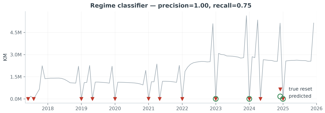
Calendar adjustment (T3) does not improve on T1 (best WAPE , MASE ), confirming that the anomalies arise from administrative processing cycles rather than month-long effects, which standard calendar adjustment is simply not designed to capture [46]. The regime-aware treatment (T4), on the other hand, is effective. Its best WAPE is and best MASE , second only to exclusion. The stage-one regime classifier, trained only on origin-available features, predicts for each month whether it is an administrative reset. When evaluated against the structural threshold labels across the expanding-window origins, it identifies the administrative resets with precision and recall of over the evaluation window, meaning that every month it flags as a reset is a true reset and it correctly identifies three of every four resets (see Figure 11); under T4 the benchmark models lead again, with several ML variants at or above (see Figure 10).
5.2. Strategy and Model Comparison Under Exclusion (T2)
Table 2 and Figure 8 present the main accuracy results under T2, the preferred evaluation framework. Exponential smoothing under the top-down strategy attains the lowest error on every metric (WAPE of , MAPE of and MASE of ), with minimum-trace reconciliation (D·ETS-MinT) a close second (WAPE ) and bottom-up ETS third. The two reconciliation variants and the leading benchmarks achieve , and thus outperform the seasonal naive reference. Regularised regression is competitive with top-down LASSO ranking fifth (WAPE , MASE ), ahead of top-down Theta and of both gradient-boosting families.
Crucially, the feature-enriched models do not surpass the benchmarks. The best Strategy C model (LightGBM-FEA, WAPE ) ranks thirteenth and XGBoost-FEA (WAPE ) seventeenth. All three Strategy C variants record . Top-down gradient boosting without microdata features performs at least as well (XGBoost, WAPE ). This indicates that the lagged microdata features add little once every predictor is required to be observable at the forecast origin. Bottom-up modelling does not improve on top-down for any model. This is consistent with the high cross-sectional correlation of the K1/K2/K3 series (Figure 1). The two low-order autoregressive benchmarks bracket this ordering instructively: the seasonal AR(1)(1)12 is competitive but sits below every exponential-smoothing and Theta variant (WAPE –), while the plain AR(1), lacking any seasonal term, is the least accurate model in the study (WAPE –). Low-order autoregression alone is thus insufficient on this strongly seasonal series, whereas the seasonal and smoothing benchmarks remain hard to beat. The per-origin WAPE distribution (Figure 8) shows ETS and MinT with both the lowest medians and the tightest spread, while the feature-enriched and gradient-boosting models show wider, heavier-tailed distributions. Example six-step forecast paths for the best model appear in Figure 9.
Figure 8.
Per-origin WAPE distribution by strategy–model combination under Treatment T2, ordered by median.
Figure 8.
Per-origin WAPE distribution by strategy–model combination under Treatment T2, ordered by median.
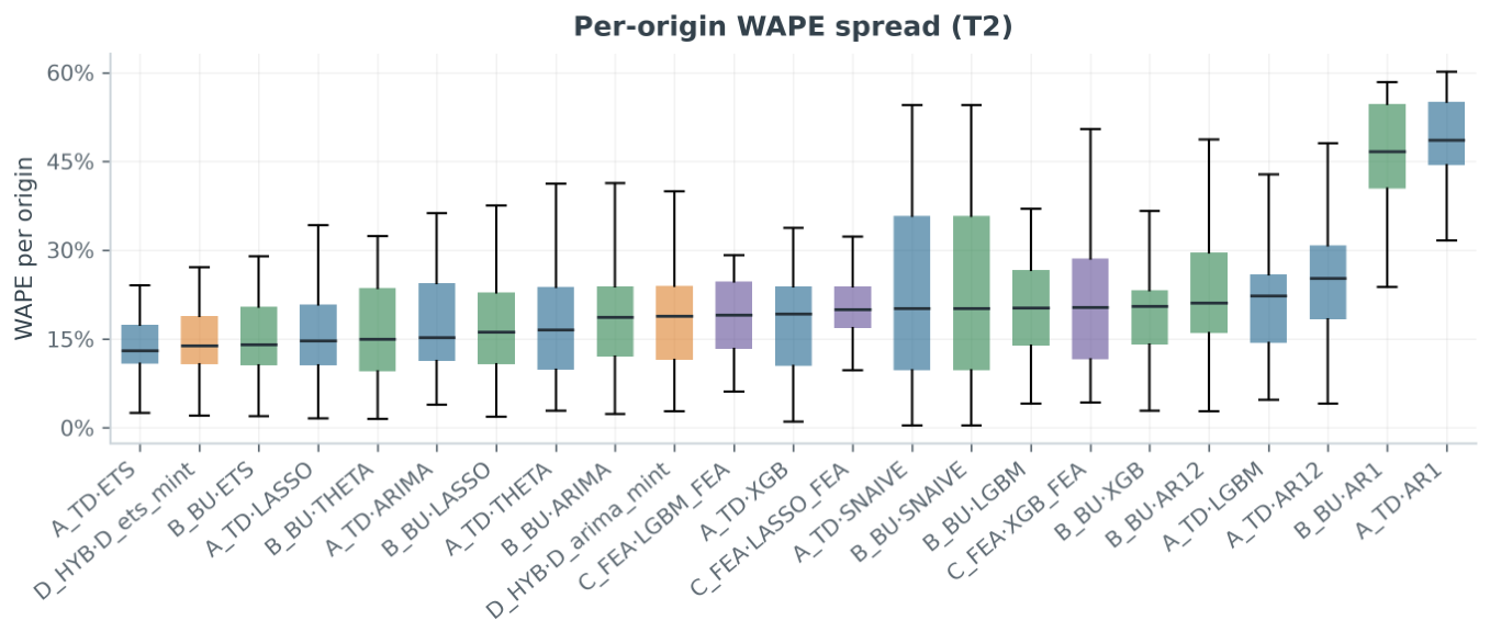
Figure 9.
Six-step-ahead forecasts (orange) against actuals (dark) for the best Treatment-T2 model (top-down ETS) at two illustrative expanding-window origins.
Figure 9.
Six-step-ahead forecasts (orange) against actuals (dark) for the best Treatment-T2 model (top-down ETS) at two illustrative expanding-window origins.
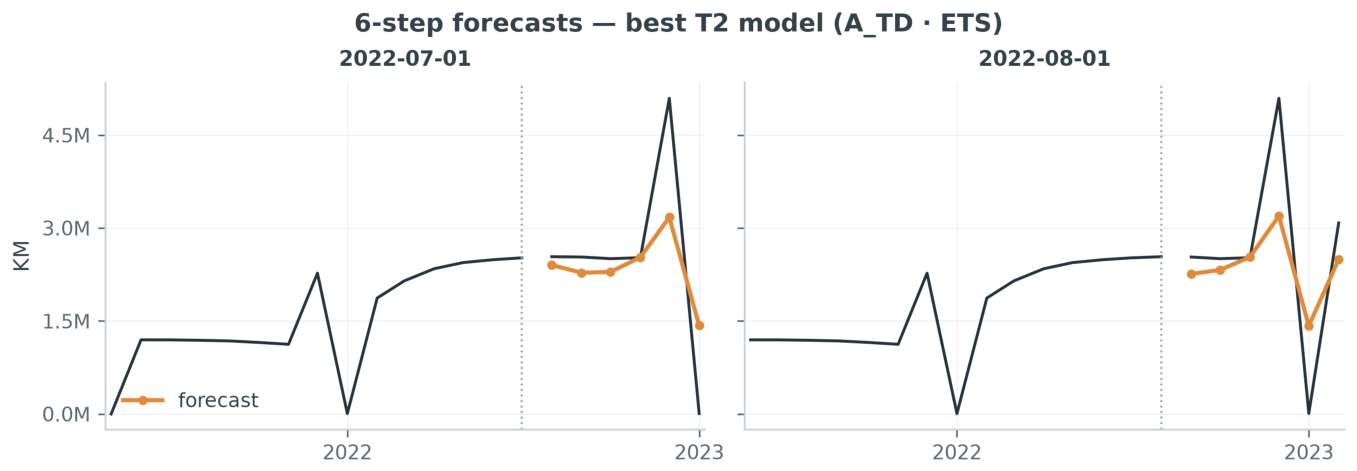
Figure 10.
Forecast skill (MASE) under Treatment T4. Values below the dashed line () outperform the seasonal naive benchmark.
Figure 10.
Forecast skill (MASE) under Treatment T4. Values below the dashed line () outperform the seasonal naive benchmark.
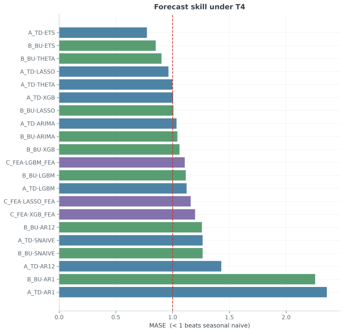
Figure 11.
Regime classifier performance. Red triangles mark true administrative resets; green circles mark months predicted anomalous by the origin-available classifier (precision , recall ).
Figure 11.
Regime classifier performance. Red triangles mark true administrative resets; green circles mark months predicted anomalous by the origin-available classifier (precision , recall ).
5.3. Statistical Comparison: Diebold-Mariano, Model Confidence Set and Friedman Test (Paired with Post-Hoc Nemenyi Analysis)
We now conduct the Diebold-Mariano (DM) statistical testing adjusted for the sample size, through the small-sample t-correction [37]. This way, we compare each model against the best performer (top-down ETS). Under the exclusion treatment (T2), a total of eleven of the nineteen comparable models are significantly worse at the level. The two plain AR(1) model benchmarks are rejected with a DM statistics of roughly 10-14 with a p-value of . These benchmark models are then followed by the gradient boosting and seasonal naive variants. Under the regime-aware treatment (T4), a total of twelve out of seventeen models are significantly worse than top-down ETS. Given the pairwise nature of the DM test, we establish that ETS beats the weaker specifications individually but does not, on its own, characterise the full field.
For a simultaneous comparison we opt for the Model Confidence Set (MCS) [38]. This framework retains the subset of models that cannot be statistically distinguished from the best at a given confidence level (refer to Table 3). At the confidence set is broad. It retains twenty models under the naive treatment and eighteen under exclusion, including every top-down and bottom-up benchmark and ML model, the seasonal AR(1)(1)12 autoregression, as well as both MinT reconciliation variants. Two exclusions might be informative. First, no feature-enriched (Strategy C) model enters the confidence set under any treatment. Second, the plain AR(1) is excluded under the preferred exclusion treatment while the seasonal AR(1)(1)12 is retained. This indicates that a low-order autoregression must carry seasonal structure to remain competitive on this series. The MCS is therefore, in a way, perimissive among the aggregate and category-level models, which are hard to distinguish from ETS on per-origin WAPE. However, as shown, the MCS draws a sharp line around the feature-enriched models and the non-seasonal autoregression.
Finally, as a third and complementary layer we apply the non-parametric procedure of Demšar [50], who applies a Friedman omnibus test followed by a Nemenyi post-hoc analysis and a critical-difference diagram (see Figure 12). The Friedman test rejects equality of mean ranks under exclusion (, ). It does so by restricting attention to the origins common to all models, so that the rank blocks are complete. The mean-rank ordering reproduces the WAPE ranking of Table 2. Top-down ETS attains the best mean rank of and is followed by ETS-MinT reconciliation and bottom-up ETS with mean ranks of and respectively. The two plain AR(1) benchmarks are, as shown, by a wide margin, the worst ( and ). At the Nemenyi critical difference is large (). This is, to be fair, a direct consequence of comparing many models over a limited number of common origins. For this reason, it does not finely separate the leading group, but it does place both AR(1) specifications, the ARIMA and LightGBM variants as well as the feature-enriched models significantly below top-down ETS.
Taken together, the three procedures, in the end, lead to a consistent conclusion. Exponential smoothing and MinT reconciliation lead in this very case, and the broad benchmark class (including seasonal autoregression) remains statistically competitive, whereas the non-seasonal low-order autoregression is the weakest approach. Finally, microdata feature enrichment never lifts the ML models into the leading group.
5.4. Accuracy over Time
We also checked whether the ranking is driven by any single period. Table 4 reports WAPE under T2 by the calendar year of the forecast target. We may notice that the ordering is relatively stable over time. In short, the top-down ETS and MinT reconciliation are the best repeatedly through all years. All models turn out to be least accurate in 2022, and over time improve monotonically. What is also interesting, and again proven, is that the feature enriched models do not improve with time; if anything their yearly WAPE goes only upward (Strategy C has no 2022 column because its first usable origin falls in 2023).
6. Discussion
6.1. When Do Simple Benchmark Models Remain Competitive?
The results of this research provide us with an insight that is very frequently discussed in forecasting literature. Complex models may provide flexibility and statistical power, but when faced with data and empirical constraints, they rarely are able to compete with simple benchmark statistical models. In other words, on a single short administrative series, simple benchmark models are clearly competitive. But besides the fact that they are competitive, they are also preferable. This is proven on the following: exponential smoothing (ETS) consistently, under all anomaly treatments, attains the lowest error (for instance T2: WAPE , MASE ); minimum-trace reconciliation is competitive to ETS, and with ETS it displays the tightest per-origin error distributions, as shown in Figure 8. Three different procedures prove this statistically: pairwise Diebold-Mariano tests [36,37], the Model Confidence Set [38] and a Friedman-Nemenyi rank analysis [50]. These procedures show that Theta and ETS lead and no machine-learning configuration displaces them. The central and much replicated finding, which is common in business and retail series that dominate the M-competitions, is again repeated here, in a public social-transfer domain far from these sector, which is that well-specified statistical benchmarks are hard to beat on short series [6,7,29]. What is interesting is that this result recurs in so different a setting, which itself, is very informative. It suggests that the benchmark advantage on short series is a structural property of the data-generating regime (few observations, strong seasonality, a policy-induced level shift), rather than an artefact of any particular application domain.
The two low-order autoregressive benchmarks may appear to contradict the above conclusion. The plain AR(1), without a seasonal term, is the least accurate model in the entire study with a WAPE between and , and is rejected by every test, whereas the seasonal AR(1)(1) is far more competitive, but still below every ETS and Theta specification (WAPE -). This shows that the autoregressive structure within these models is not the one responsible for the benchmark superiority. What is responsible, on the other hand, is the parsimonious joint modelling of trend and seasonality embodied in ETS and Theta. This distinction is very much transparent in the Theta method, which is equivalent to simple ETS with drift [24]. However, this reading is nonetheless warranted: the Model Confidence Set is broad with eighteen models under exclusion, so we do not claim unique statistical superiority for exponential smoothing. The practical case rests on its lowest point error, tightest dispersion, parsimony and negligible computational cost.
6.2. Does Enriching the Models Add Value?
Whether richer information overturns benchmark models’ dominance is a complementary question to the one discussed in the previous subsection. However, the answer appears to be more or less negative. Predictors engineered from million individual payment records, unfortunately fail to improve on the plain aggregate models whatsoever. No feature-enriched model attains , none enters the Model Confidence Set under any of the treatments and top-down gradient boosting without microdata performs at least as well, which isolates the marginal value of the microdata as essentially none once every predictor is contrained to be observable at the forecast origin.
This outcome is aligned, and helps further explain, the boundary conditions established in the recent ML forecasting literature. Machine learning tends to beat statistical benchmarks when it can exploit cross-series structure, for instance learning a single global model across many related series [51], or, for example, when the series share exploitable characteristics such as related seasonal patterns and sufficient length [52]. Unfortunately, none of these conditions hold in our setting. Firstly, our forecasting target is a single aggregate series, and the three disaggraegate categories are near-collinear rather than heterogeneous, and thus there are no cross-learning opportunities. The microdata, moreover, is informative largely because it is contemporaneous, so once lagged to respect the information set, their marginal content over the target’s own history and seasonality is small.
6.3. Aggregation, Anomaly Treatment, Cost and Limitations
Three secondary results happen to reinforce our main finding. Regarding aggregation, bottom-up modeling in Strategy B does not improve on top-down (Strategy A) for any model whatsoever. This is beacuse K1, K2 and K3 share indexation base, beneficiary population pool and payment calendar and are (thus) near collinear (see Figure 1). As a result, disaggregation adds estimation noise without any predictive value. Where the hierarchy does help is through reconciliation rather than summation. Minimum trace reconciliation [19] matches the best top-down model and the confidence set retains it, so in general, the practical lesson is to reconcile rather than sum, and to also expect only modest gains when the disaggregate series are highly correlated.
When it comes to anomaly treatment, the crucial aspect is handling of the near-zero and zero anomalous months. Naive scoring inflates MAPE beyond several thousand percent due to the said anomalous degeneracy, which motivated the scale-free measures of Hyndman and Koehler [14]. This is why we emphasize weighted and scaled errors throughout. Calendar adjustment (T3) was proven ineffective because the anomalies are institutional rather than calendar-length in origin, which is yet again impossible to capture by standard adjustment methods [46]. On the other hand, the regime-aware treatment (T4) is effective with the best WAPE of , MASE of . The way how this was handled was that a simple origin-available classifier detected the resets with precision and recall and assigned them their historical near-zero level. For any series with administrative zero-periods such as payment systems, procurement cycles and seasonal programs, we recommend excluding the anomalous months from scoring. If exclusion is not an option, then we recommend handling them through an explicit regime step and reporting scaled rather than percentage errors.
On a more technical note, the cost and operational use of the software in fitting these models is worth mentioning. The benchmark models fit in well under a second per origin, whereas the recursive ML models ran up to forty minutes for the full evaluation on a Macbook Pro M2. As the benchmarks are simultaneously the most accurate, the ML models here provide no added value, since they are significantly slower and no better than benchmarks. This aligns with the cost concern by Makridakis et al. [9].
Several limitations qualify these conclusions. First, the results pertain to a single government’s child benefit programme, so generalisation might require further evidence. Next, the ML set is here representative and compared to benchmark set. This is why deeper learning architectures are omitted, as they exploit rather long histories or cross-learning across many related series [51,52], and these conditions are absent here. This is why their inclusion would be inappropriate and unnecessary. Moreover, the microdata lagged features often understate the value of genuinely leading indicators (for instance the counts of pending or approved-but-unpaid entitlements) that a richer administrative linkage may supply. Finally, the evaluation spans 38 expanding-window origins on a 103 month series. The overlapping origins mean the Friedman-Nemenyi analysis is read as a verification rather than exact independent inference, and a longer series would show how accuracy changes with the horizon and whether reconciliation helps.
7. Conclusions
The main question of this research was whether simple benchmark models are competitive in forecasting social protection expenditures but also whether richer, feature-enriched information adds predictive value. This was done using monthly child-benefit expenditure in Republika Srpska with a short aggregate series of 103 observations supported by million individual payment records. Four forecasting strategies of increasing informational richness were compared across a common set of benchmark and ML models, under an expanding window design in which every predictor is observable at the forecast origin and also across four treatments of the administrative calendar anomalies characteristic of payment data.
Three conclusions follow. First, the general idea is that, according to the findings resulted from this research, benchmark models remain preferable on short, correlated, strongly seasonal series. Exponential smoothing (ETS), in this case, turns out to be by far the most accurate model under every one of the anomaly treatments (WAPE , MASE under exclusion), whereas MinT performs just as well. This ordering is confirmed statistically by Diebold-Mariano tests, the Model Confidence Set and a Friedman-Nemenyi analysis. Seasonal low order autoregression runs close and is competitive, wheres plain AR(1) is the least accurate model in the study. This proves that the parsimonous modelling of seasonality and trend makes the benchmark class hard to beat, not really the autoregressive structure alone [7,29]. Second, on this specific short time-series data, the microdata available, once restricted and controlled to the forecast origin, appears to add incremental to no predictive value at the aggregate level. This is visible through the fact that no feature-enriched model enters the Model Confidence Set, and that the gradient boosting without microdata performs at least as well. This stays consistent with the boundary conditions under which ML is known to succeed, namely cross-learning and genuinely leading informating, none of which is present for a single aggregate series with near-collinear components [51,52]. Finally, the treatment of calendar anomalies matters in its own right. Naive percentage-error evaluation is unusable, while the exclusion and regime-aware treatments give stable rankings, which is a caution that applies to any series with such (institutional) anomalies, i.e. institutional zero-periods.
Author Contributions
Conceptualisation, A.Š. and B.B.; methodology, A.Š.; software, A.Š.; validation, A.Š. and B.B.; formal analysis, A.Š.; investigation, A.Š., B.B. and D.M.; data curation, A.Š. and V.L.; writing—original draft preparation, A.Š.; writing—review and editing, A.Š. and B.B.; supervision, B.B. All authors have read and agreed to the published version of the manuscript.
Funding
This research received no external funding.
Institutional Review Board Statement
Not applicable.
Informed Consent Statement
Not applicable.
Data Availability Statement
The administrative microdata underlying this study were provided by the Public Child Protection Fund of Republika Srpska under a data-sharing agreement and are not publicly available due to privacy restrictions. Aggregated monthly series and the Pythom script used for the analysis are available from the corresponding author upon reasonable request.
Acknowledgments
The authors thank the Public Child Protection Fund of Republika Srpska for providing access to the administrative data. The authors have reviewed and edited all outputs and take full responsibility for the content of this publication.
Conflicts of Interest
The authors declare no conflicts of interest.
Abbreviations
The following abbreviations are used in this manuscript:
| ARIMA | Autoregressive Integrated Moving Average |
| BU | Bottom-Up |
| CV | Cross-Validation |
| DM | Diebold–Mariano |
| ETS | Error-Trend-Seasonality (exponential smoothing) |
| FEA | Feature-Enriched Aggregate |
| KM | Convertible Mark (currency of Bosnia and Herzegovina) |
| LASSO | Least Absolute Shrinkage and Selection Operator |
| ML | Machine Learning |
| MAPE | Mean Absolute Percentage Error |
| MASE | Mean Absolute Scaled Error |
| MCS | Model Confidence Set |
| MinT | Minimum Trace (reconciliation) |
| RMSSE | Root Mean Squared Scaled Error |
| RS | Republika Srpska |
| TD | Top-Down |
| WAPE | Weighted Absolute Percentage Error |
References
- Kara, B.; Şengüler, H. A Comparative Analysis of Budget Forecasting Methods: A Systematic Literature Review Covering the 1983–2024 Period. Public Budgeting & Finance 2025, 46, 29–46. [CrossRef]
- JU Javni fond za dječiju zaštitu Republike Srpske. Godišnji izvještaj o isplatama prava na dodatak na djecu, 2024.
- Vlada Republike Srpske. Odluka o utvrđivanju osnovice za visinu dječijeg dodatka za 2024. godinu, 2024. Službeni glasnik Republike Srpske, 2024.
- Ghysels, E.; Ozkan, N. Real-time forecasting of the US federal government budget: A simple mixed frequency data regression approach. International Journal of Forecasting 2015, 31, 1009–1020. [CrossRef]
- Hyndman, R.J.; Athanasopoulos, G. Forecasting: Principles and Practice, 3rd ed.; OTexts: Melbourne, Australia, 2021.
- Makridakis, S.; Hibon, M. The M3-Competition: results, conclusions and implications. International Journal of Forecasting 2000, 16, 451–476. [CrossRef]
- Makridakis, S.; Spiliotis, E.; Assimakopoulos, V. The M4 Competition: 100,000 Time Series and 61 Forecasting Methods. International Journal of Forecasting 2020, 36, 54–74. [CrossRef]
- Makridakis, S.; Spiliotis, E.; Assimakopoulos, V. M5 Accuracy Competition: Results, Findings, and Conclusions. International Journal of Forecasting 2022, 38, 1346–1364. [CrossRef]
- Makridakis, S.; Spiliotis, E.; Assimakopoulos, V. Statistical and Machine Learning Forecasting Methods: Concerns and Ways Forward. PLOS ONE 2018, 13, e0194889. [CrossRef]
- Swenson, C. Using Machine Deep Learning AI to Improve Forecasting of Tax Payments for Corporations. Forecasting 2024, 6, 968–984. [CrossRef]
- Larson, S.E.; Overton, M. Modeling Approach Matters, But Not as Much as Preprocessing: Comparison of Machine Learning and Traditional Revenue Forecasting Techniques. Public Finance Journal 2024, 1, 29–48. [CrossRef]
- Smyl, S. A hybrid method of exponential smoothing and recurrent neural networks for time series forecasting. International Journal of Forecasting 2020, 36, 75–85. [CrossRef]
- Montero-Manso, P.; Athanasopoulos, G.; Hyndman, R.J.; Talagala, T.S. FFORMA: Feature-based forecast model averaging. International Journal of Forecasting 2020, 36, 86–92. [CrossRef]
- Hyndman, R.J.; Koehler, A.B. Another Look at Measures of Forecast Accuracy. International Journal of Forecasting 2006, 22, 679–688. [CrossRef]
- Kaufman, S.; Rosset, S.; Perlich, C.; Stitelman, O. Leakage in data mining: Formulation, detection, and avoidance. ACM Transactions on Knowledge Discovery from Data 2012, 6, 1–21. [CrossRef]
- Kapoor, S.; Narayanan, A. Leakage and the reproducibility crisis in machine-learning-based science. Patterns 2023, 4, 100804. [CrossRef]
- Tashman, L.J. Out-of-sample tests of forecasting accuracy: an analysis and review. International Journal of Forecasting 2000, 16, 437–450. [CrossRef]
- Bergmeir, C.; Benítez, J.M. On the use of cross-validation for time series predictor evaluation. Information Sciences 2012, 191, 192–213. [CrossRef]
- Wickramasuriya, S.L.; Athanasopoulos, G.; Hyndman, R.J. Optimal Forecast Reconciliation for Hierarchical and Grouped Time Series Through Trace Minimization. Journal of the American Statistical Association 2019, 114, 804–819. [CrossRef]
- Hyndman, R.J.; Koehler, A.B.; Ord, J.K.; Snyder, R.D. Forecasting with Exponential Smoothing: The State Space Approach; Springer: Berlin, Heidelberg, 2008. [CrossRef]
- Hyndman, R.J.; Khandakar, Y. Automatic Time Series Forecasting: The forecast Package for R. Journal of Statistical Software 2008, 27, 1–22. [CrossRef]
- Box, G.E.P.; Jenkins, G.M.; Reinsel, G.C.; Ljung, G.M. Time Series Analysis: Forecasting and Control, 5th ed.; John Wiley & Sons: Hoboken, NJ, 2015.
- Assimakopoulos, V.; Nikolopoulos, K. The theta model: a decomposition approach to forecasting. International Journal of Forecasting 2000, 16, 521–530. [CrossRef]
- Hyndman, R.J.; Billah, B. Unmasking the Theta method. International Journal of Forecasting 2003, 19, 287–290. [CrossRef]
- Tibshirani, R. Regression Shrinkage and Selection via the LASSO. Journal of the Royal Statistical Society: Series B 1996, 58, 267–288. [CrossRef]
- Chen, T.; Guestrin, C. XGBoost: A Scalable Tree Boosting System. In Proceedings of the Proceedings of the 22nd ACM SIGKDD International Conference on Knowledge Discovery and Data Mining, 2016, pp. 785–794. [CrossRef]
- Ke, G.; Meng, Q.; Finley, T.; Wang, T.; Chen, W.; Ma, W.; Ye, Q.; Liu, T.Y. LightGBM: A Highly Efficient Gradient Boosting Decision Tree. In Proceedings of the Advances in Neural Information Processing Systems 30 (NeurIPS), 2017, pp. 3146–3154.
- Januschowski, T.; Gasthaus, J.; Wang, Y.; Salinas, D.; Flunkert, V.; Bohlke-Schneider, M.; Callot, L. Criteria for classifying forecasting methods. International Journal of Forecasting 2020, 36, 167–177. [CrossRef]
- Petropoulos, F.; Apiletti, D.; Assimakopoulos, V.; et al. Forecasting: Theory and Practice. International Journal of Forecasting 2022, 38, 705–871. [CrossRef]
- Hyndman, R.J.; Ahmed, R.A.; Athanasopoulos, G.; Shang, H.L. Optimal Combination Forecasts for Hierarchical Time Series. Computational Statistics & Data Analysis 2011, 55, 2579–2589. [CrossRef]
- Athanasopoulos, G.; Ahmed, R.A.; Hyndman, R.J. Hierarchical forecasts for Australian domestic tourism. International Journal of Forecasting 2009, 25, 146–166. [CrossRef]
- Athanasopoulos, G.; Hyndman, R.J.; Kourentzes, N.; Petropoulos, F. Forecasting with temporal hierarchies. European Journal of Operational Research 2017, 262, 60–74. [CrossRef]
- Panagiotelis, A.; Gamakumara, P.; Athanasopoulos, G.; Hyndman, R.J. Probabilistic forecast reconciliation: Properties, evaluation and score optimisation. European Journal of Operational Research 2023, 306, 693–706. [CrossRef]
- Athanasopoulos, G.; Hyndman, R.J.; Kourentzes, N.; Panagiotelis, A. Forecast Reconciliation: A Review. International Journal of Forecasting 2024, 40, 430–456. [CrossRef]
- Athanasopoulos, G.; Kourentzes, N. On the evaluation of hierarchical forecasts. International Journal of Forecasting 2023, 39, 1502–1511. [CrossRef]
- Diebold, F.X.; Mariano, R.S. Comparing Predictive Accuracy. Journal of Business & Economic Statistics 1995, 13, 253–263. [CrossRef]
- Harvey, D.; Leybourne, S.; Newbold, P. Testing the Equality of Prediction Mean Squared Errors. International Journal of Forecasting 1997, 13, 281–291. [CrossRef]
- Hansen, P.R.; Lunde, A.; Nason, J.M. The Model Confidence Set. Econometrica 2011, 79, 453–497. [CrossRef]
- Bergmeir, C.; Hyndman, R.J.; Koo, B. A note on the validity of cross-validation for evaluating autoregressive time series prediction. Computational Statistics & Data Analysis 2018, 120, 70–83. [CrossRef]
- Cerqueira, V.; Torgo, L.; Mozetič, I. Evaluating Time Series Forecasting Models: An Empirical Study on Performance Estimation Methods. Machine Learning 2020, 109, 1997–2028. [CrossRef]
- Plotnick, R.D.; Lidman, R.M. Forecasting Welfare Caseloads: A Tool to Improve Budgeting. Public Budgeting & Finance 1987, 7, 70–81. [CrossRef]
- Fantazzini, D. Nowcasting and Forecasting the Monthly Food Stamps Data in the US Using Online Search Data. PLoS ONE 2014, 9, e111894. [CrossRef]
- Hayashi, M. Forecasting welfare caseloads: The case of the Japanese public assistance program. Socio-Economic Planning Sciences 2014, 48, 105–114. [CrossRef]
- Immervoll, H.; Richardson, L. Redistribution Policy and Inequality Reduction in OECD Countries: What Has Changed in Two Decades? OECD Social, Employment and Migration Working Papers 2018. [CrossRef]
- Larson, W.D.; Sinclair, T.M. Nowcasting unemployment insurance claims in the time of COVID-19. International Journal of Forecasting 2022, 38, 635–647. [CrossRef]
- Eurostat. JDemetra+ Seasonal Adjustment Software: Methodological Guidelines. Technical report, European Commission, Eurostat, Luxembourg, 2024.
- Narodna skupština Republike Srpske. Zakon o dječijoj zaštiti Republike Srpske, 2002. Službeni glasnik Republike Srpske, br. 4/2002, sa izmjenama.
- Narodna skupština Republike Srpske. Zakon o izmjenama i dopunama Zakona o dječijoj zaštiti, 2022. Službeni glasnik Republike Srpske, br. 1/2022.
- Bojer, C.S.; Meldgaard, J.P. Kaggle forecasting competitions: An overlooked learning opportunity. International Journal of Forecasting 2021, 37, 587–603. [CrossRef]
- Demšar, J. Statistical Comparisons of Classifiers over Multiple Data Sets. Journal of Machine Learning Research 2006, 7, 1–30.
- Montero-Manso, P.; Hyndman, R.J. Principles and algorithms for forecasting groups of time series: Locality and globality. International Journal of Forecasting 2021, 37, 1632–1653. [CrossRef]
- Hewamalage, H.; Bergmeir, C.; Bandara, K. Global models for time series forecasting: A simulation study. Pattern Recognition 2022, 124, 108441. [CrossRef]
Figure 1.
The three category series K1, K2, and K3 (the bottom level of the forecasting hierarchy) after point-in-time attribution.
Figure 1.
The three category series K1, K2, and K3 (the bottom level of the forecasting hierarchy) after point-in-time attribution.
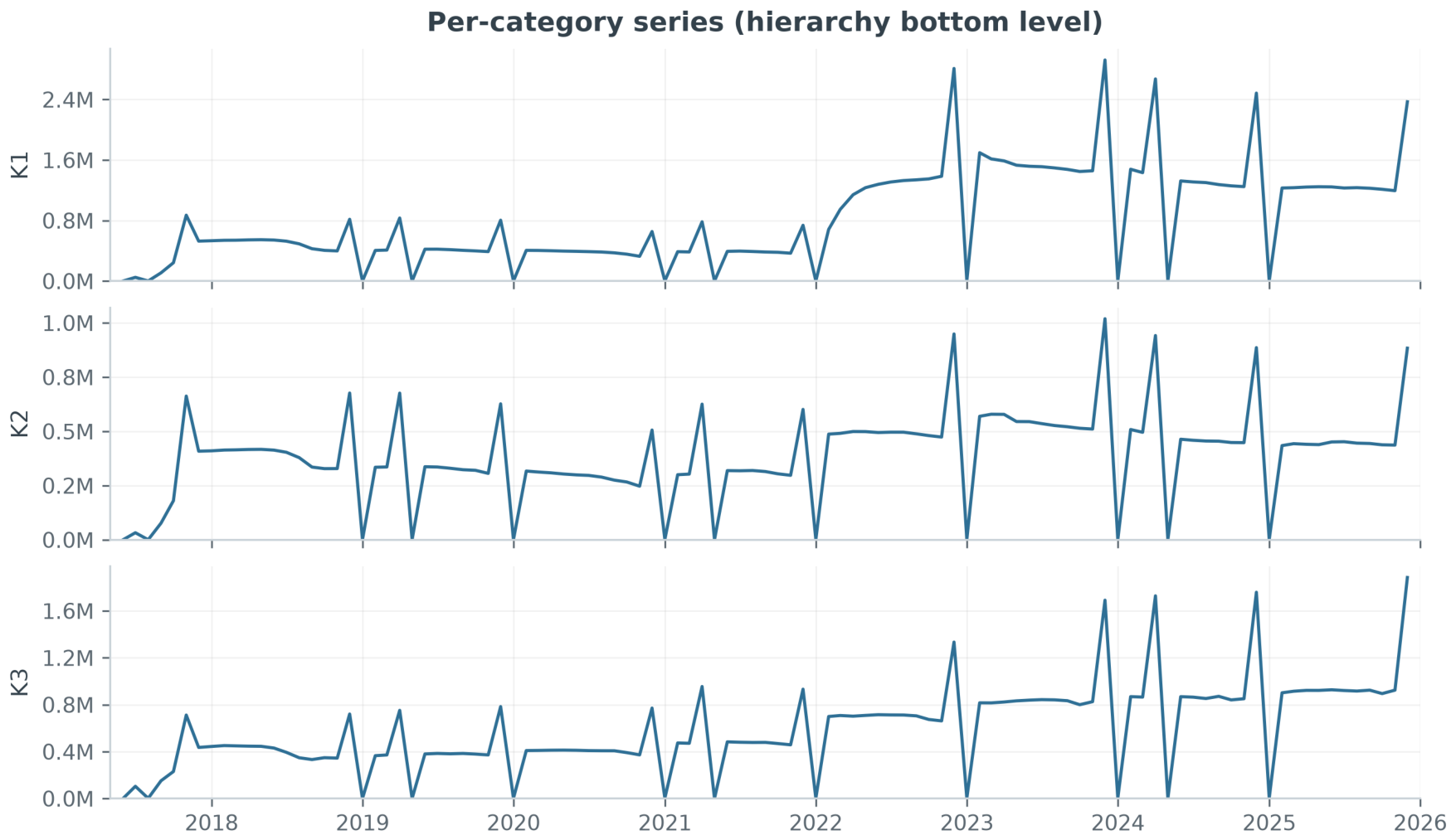
Figure 2.
Isolation-Forest anomaly scores; circled months coincide with the administrative-reset months identified by the structural threshold.
Figure 2.
Isolation-Forest anomaly scores; circled months coincide with the administrative-reset months identified by the structural threshold.
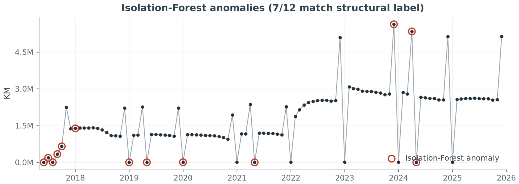
Figure 3.
Methodological overview. Transaction-level microdata are attributed to benefit categories by a point-in-time join and aggregated to the monthly target series, with anomalous reset months flagged by a first-window-calibrated threshold . All predictors are constructed to be observable at the forecast origin. Four forecasting strategies (A–D) are each evaluated under four anomaly treatments (T1–T4) in an expanding-window cross-validation, and compared through three statistical procedures. Strategies C and D use only the treatments for which they are defined (C: all four; D: T1 and T2).
Figure 3.
Methodological overview. Transaction-level microdata are attributed to benefit categories by a point-in-time join and aggregated to the monthly target series, with anomalous reset months flagged by a first-window-calibrated threshold . All predictors are constructed to be observable at the forecast origin. Four forecasting strategies (A–D) are each evaluated under four anomaly treatments (T1–T4) in an expanding-window cross-validation, and compared through three statistical procedures. Strategies C and D use only the treatments for which they are defined (C: all four; D: T1 and T2).
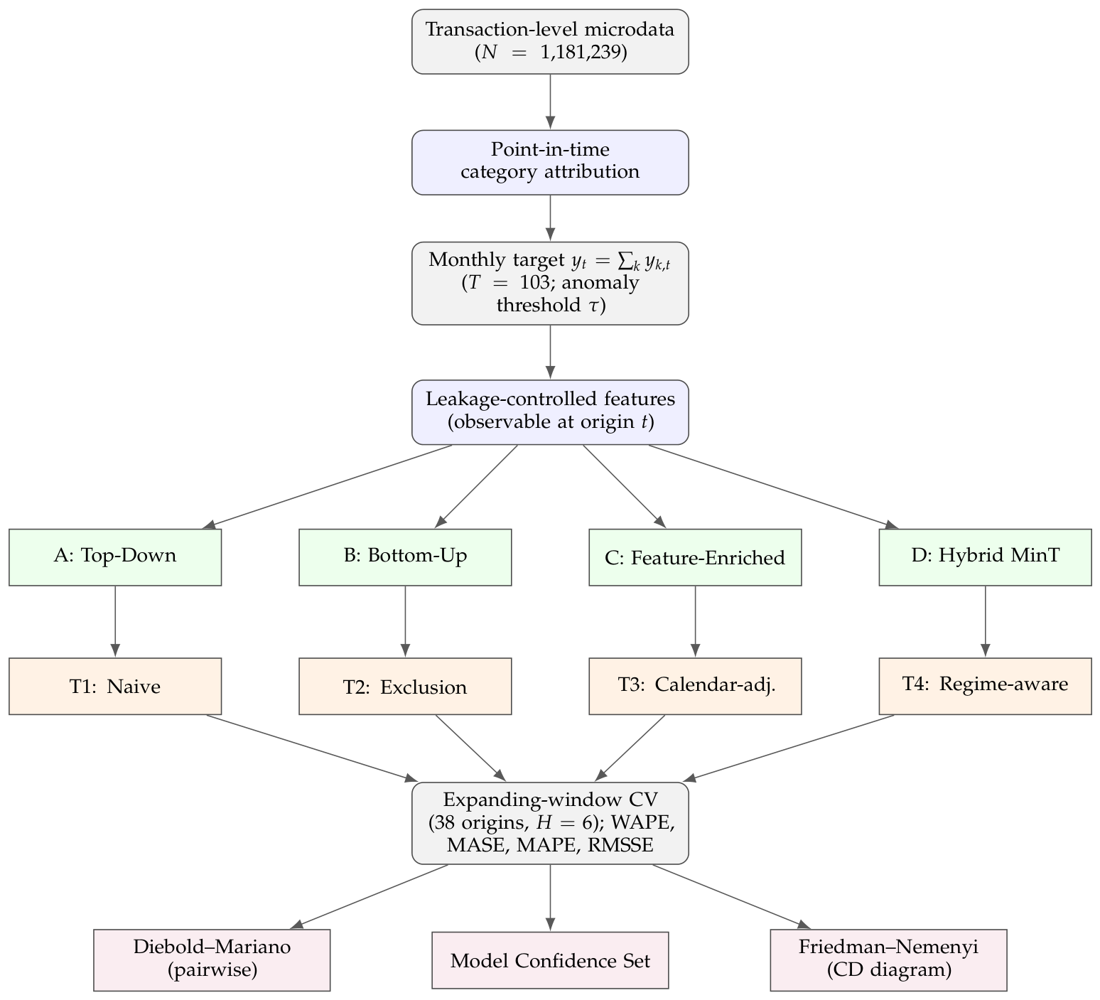
Figure 4.
Leakage-controlled predictor design. For a forecast issued at origin t, every predictor of the target month is drawn from feature months at or before t, i.e. within the information set available at the origin.
Figure 4.
Leakage-controlled predictor design. For a forecast issued at origin t, every predictor of the target month is drawn from feature months at or before t, i.e. within the information set available at the origin.
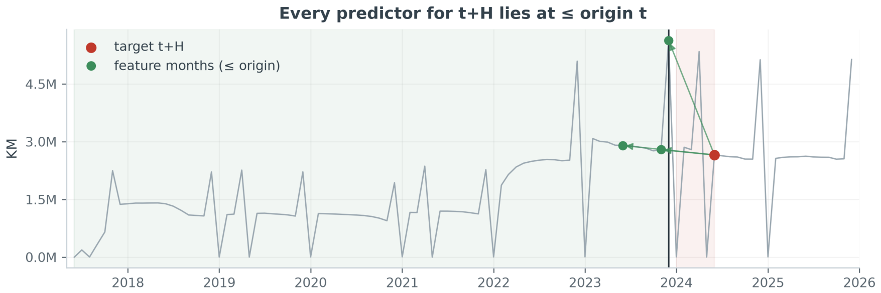
Figure 5.
Expanding-window evaluation. Each row is one origin: the training window (blue) grows by one month per origin; the six-month test block (orange, ) follows the origin.
Figure 5.
Expanding-window evaluation. Each row is one origin: the training window (blue) grows by one month per origin; the six-month test block (orange, ) follows the origin.
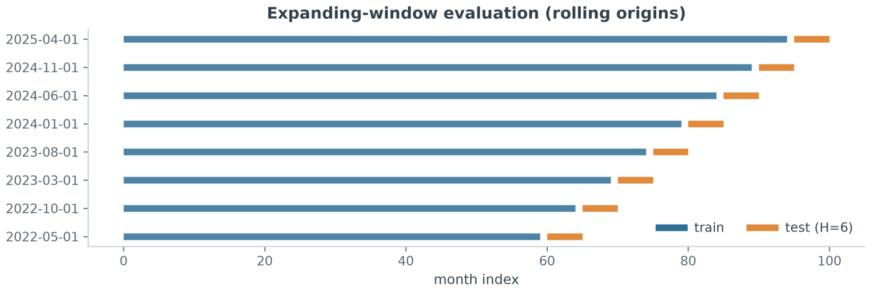
Figure 6.
Mean WAPE by strategy–model combination (rows) and anomaly treatment (columns); lower is better. Blank cells denote combinations not defined for a treatment; minimum-trace reconciliation (D) is applied only under the naive and exclusion treatments.
Figure 6.
Mean WAPE by strategy–model combination (rows) and anomaly treatment (columns); lower is better. Blank cells denote combinations not defined for a treatment; minimum-trace reconciliation (D) is applied only under the naive and exclusion treatments.
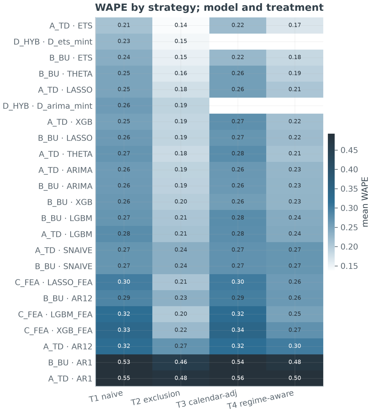
Figure 7.
Best-model WAPE per strategy under each anomaly treatment. Exclusion (T2) yields the lowest errors and the regime-aware treatment (T4) the second-lowest; the feature-enriched strategy (C) is worst under every treatment.
Figure 7.
Best-model WAPE per strategy under each anomaly treatment. Exclusion (T2) yields the lowest errors and the regime-aware treatment (T4) the second-lowest; the feature-enriched strategy (C) is worst under every treatment.
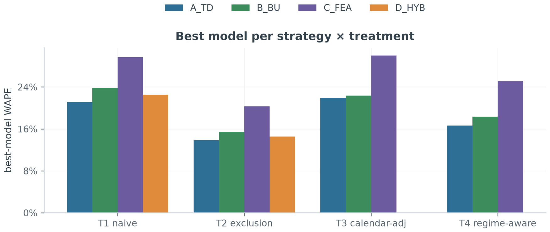
Figure 12.
Critical-difference diagram under Treatment T2 (Friedman , ; Nemenyi , ). Points are mean ranks across the common evaluation origins (lower is better); horizontal bars connect models whose mean ranks differ by less than the critical difference.
Figure 12.
Critical-difference diagram under Treatment T2 (Friedman , ; Nemenyi , ). Points are mean ranks across the common evaluation origins (lower is better); horizontal bars connect models whose mean ranks differ by less than the critical difference.
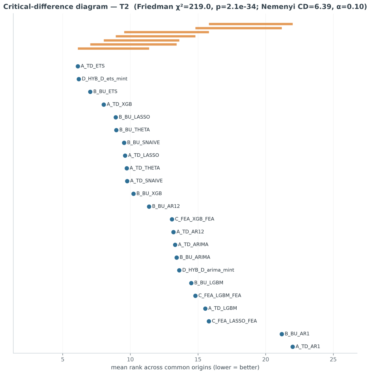

Table 1.
Machine-learning hyperparameters, held fixed across all origins, treatments and strategies. These are standard, lightly regularised defaults rather than tuned optima, which is appropriate given the series length and consistent with our aim of testing whether any off-the-shelf configuration overturns the benchmark ordering.
Table 1.
Machine-learning hyperparameters, held fixed across all origins, treatments and strategies. These are standard, lightly regularised defaults rather than tuned optima, which is appropriate given the series length and consistent with our aim of testing whether any off-the-shelf configuration overturns the benchmark ordering.
| Model | Setting | Value |
| XGBoost | Objective | Squared error |
| Number of trees | 300 | |
| Maximum tree depth | 4 | |
| Learning rate | ||
| Row / column subsampling | / | |
| LightGBM | Objective | Regression (L2) |
| Number of trees | 300 | |
| Learning rate | ||
| Number of leaves | 15 | |
| Min. obs. per leaf / row subsampling | 5 / | |
| LASSO | Predictor scaling | Standardised per training window |
| Penalty () | Selected by 5-fold CV | |
| Regularisation path | 50 candidate values of |
Table 2.
Mean forecast accuracy under Treatment T2 (Exclusion), expanding-window cross-validation, non-anomalous months only, ordered by WAPE.
Table 2.
Mean forecast accuracy under Treatment T2 (Exclusion), expanding-window cross-validation, non-anomalous months only, ordered by WAPE.
| Strategy | Model | MAPE | WAPE | MASE | RMSSE |
|---|---|---|---|---|---|
| A: Top-Down | ETS | 11.9% | 13.9% | 0.755 | 0.740 |
| D: Hybrid-MinT | ETS-MinT | 12.9% | 14.5% | 0.791 | 0.733 |
| B: Bottom-Up | ETS | 14.1% | 15.4% | 0.843 | 0.765 |
| B: Bottom-Up | Theta | 14.4% | 16.3% | 0.898 | 0.826 |
| A: Top-Down | LASSO | 16.0% | 17.6% | 0.948 | 0.845 |
| A: Top-Down | Theta | 16.3% | 18.1% | 0.999 | 0.882 |
| A: Top-Down | XGBoost | 17.0% | 18.6% | 1.003 | 0.936 |
| B: Bottom-Up | LASSO | 17.4% | 18.9% | 0.998 | 0.888 |
| A: Top-Down | ARIMA | 18.2% | 19.0% | 1.008 | 0.886 |
| D: Hybrid-MinT | ARIMA-MinT | 18.0% | 19.1% | 1.018 | 0.880 |
| B: Bottom-Up | ARIMA | 18.0% | 19.2% | 1.028 | 0.886 |
| B: Bottom-Up | XGBoost | 18.1% | 19.8% | 1.055 | 0.952 |
| C: Feature-Enriched | LightGBM-FEA | 19.3% | 20.3% | 1.054 | 0.968 |
| B: Bottom-Up | LightGBM | 18.7% | 20.7% | 1.112 | 1.028 |
| C: Feature-Enriched | LASSO-FEA | 20.1% | 20.8% | 1.090 | 0.866 |
| A: Top-Down | LightGBM | 19.4% | 21.1% | 1.120 | 1.016 |
| C: Feature-Enriched | XGBoost-FEA | 21.4% | 22.2% | 1.115 | 0.942 |
| B: Bottom-Up | AR(1)(1)12 | 21.7% | 23.3% | 1.274 | 1.127 |
| A: Top-Down | SNAIVE | 23.0% | 23.6% | 1.281 | 1.084 |
| B: Bottom-Up | SNAIVE | 23.0% | 23.6% | 1.281 | 1.084 |
| A: Top-Down | AR(1)(1)12 | 25.4% | 26.9% | 1.472 | 1.241 |
| B: Bottom-Up | AR(1) | 43.3% | 45.7% | 2.460 | 1.880 |
| A: Top-Down | AR(1) | 45.7% | 48.0% | 2.585 | 1.953 |
MAPE and WAPE as percentages. indicates outperformance of the seasonal naive benchmark. Bold = best per metric. AR(1) and AR(1)(1)12 are fixed-order low-order autoregressive benchmarks. Strategies A, B, and D are evaluated over 38 origins; the feature-enriched Strategy C over 26 origins.
Table 3.
Model Confidence Set membership at : ✓ = retained, ✘ = excluded, — = not defined for that treatment. The number of retained models is 20 (T1) and 18 (T2, T3, T4).
Table 3.
Model Confidence Set membership at : ✓ = retained, ✘ = excluded, — = not defined for that treatment. The number of retained models is 20 (T1) and 18 (T2, T3, T4).
| Strategy | Model | T1 | T2 | T3 | T4 |
|---|---|---|---|---|---|
| A: Top-Down | ETS | ✓ | ✓ | ✓ | ✓ |
| A: Top-Down | Theta | ✓ | ✓ | ✓ | ✓ |
| A: Top-Down | ARIMA | ✓ | ✓ | ✓ | ✓ |
| A: Top-Down | LASSO | ✓ | ✓ | ✓ | ✓ |
| A: Top-Down | XGBoost | ✓ | ✓ | ✓ | ✓ |
| A: Top-Down | LightGBM | ✓ | ✓ | ✓ | ✓ |
| A: Top-Down | SNAIVE | ✓ | ✓ | ✓ | ✓ |
| A: Top-Down | AR(1)(1)12 | ✓ | ✓ | ✓ | ✓ |
| A: Top-Down | AR(1) | ✓ | ✘ | ✓ | ✓ |
| B: Bottom-Up | ETS | ✓ | ✓ | ✓ | ✓ |
| B: Bottom-Up | Theta | ✓ | ✓ | ✓ | ✓ |
| B: Bottom-Up | ARIMA | ✓ | ✓ | ✓ | ✓ |
| B: Bottom-Up | LASSO | ✓ | ✓ | ✓ | ✓ |
| B: Bottom-Up | XGBoost | ✓ | ✓ | ✓ | ✓ |
| B: Bottom-Up | LightGBM | ✓ | ✓ | ✓ | ✓ |
| B: Bottom-Up | SNAIVE | ✓ | ✓ | ✓ | ✓ |
| B: Bottom-Up | AR(1)(1)12 | ✓ | ✓ | ✓ | ✓ |
| B: Bottom-Up | AR(1) | ✓ | ✘ | ✓ | ✓ |
| C: Feature-Enriched | XGBoost-FEA | ✘ | ✘ | ✘ | ✘ |
| C: Feature-Enriched | LightGBM-FEA | ✘ | ✘ | ✘ | ✘ |
| C: Feature-Enriched | LASSO-FEA | ✘ | ✘ | ✘ | ✘ |
| D: Hybrid-MinT | ETS-MinT | ✓ | ✓ | — | — |
| D: Hybrid-MinT | ARIMA-MinT | ✓ | ✓ | — | — |
The feature-enriched (C) models are excluded under every treatment; the plain AR(1) is excluded under exclusion (T2); the MinT reconciliation (D) is defined only for the naive and exclusion treatments.
Table 4.
WAPE (%) under Treatment T2 by forecast-target year, selected models. The 2022 column rests on fewer origins (evaluation begins 2022:05).
Table 4.
WAPE (%) under Treatment T2 by forecast-target year, selected models. The 2022 column rests on fewer origins (evaluation begins 2022:05).
| Strategy | Model | 2022 | 2023 | 2024 | 2025 |
|---|---|---|---|---|---|
| A: Top-Down | ETS | 19.4 | 12.9 | 14.3 | 10.8 |
| D: Hybrid-MinT | ETS-MinT | 20.0 | 14.2 | 14.9 | 10.5 |
| B: Bottom-Up | ETS | 23.4 | 15.2 | 15.1 | 10.5 |
| A: Top-Down | XGBoost | 26.8 | 19.0 | 17.2 | 14.0 |
| C: Feature-Enr. | LightGBM-FEA | — | 15.3 | 21.8 | 20.2 |
| C: Feature-Enr. | XGBoost-FEA | — | 16.6 | 20.5 | 26.8 |
| A: Top-Down | AR(1) | 59.3 | 53.4 | 48.0 | 34.5 |
Disclaimer/Publisher’s Note: The statements, opinions and data contained in all publications are solely those of the individual author(s) and contributor(s) and not of MDPI and/or the editor(s). MDPI and/or the editor(s) disclaim responsibility for any injury to people or property resulting from any ideas, methods, instructions or products referred to in the content. |
© 2026 by the authors. Licensee MDPI, Basel, Switzerland. This article is an open access article distributed under the terms and conditions of the Creative Commons Attribution (CC BY) license (http://creativecommons.org/licenses/by/4.0/).
Copyright: This open access article is published under a Creative Commons CC BY 4.0 license, which permit the free download, distribution, and reuse, provided that the author and preprint are cited in any reuse.