

Submitted:
16 October 2026
Posted:
20 October 2026
You are already at the latest version
Abstract
Bone density at the implant site is still assessed subjectively, with high inter- and intra-observer variability. This ex vivo study evaluated the repeatability of electrochemical impedance spectroscopy (EIS) of bone and its correlation with implant primary stability, measured by resonance frequency analysis (ISQ). Thirty bovine bone samples, each from a different animal, underwent triplicate EIS scans (3–99.1 kHz) within 6 h post-mortem; the Quality Bone Parameter (QBP) was defined as the base-10 logarithm of the impedance modulus at 99.1 kHz. A 3.8 × 10 mm implant was then placed after standardized drilling, and ISQ was measured immediately. Two samples with non-physical acquisitions (negative real impedance) were excluded. In the remaining 28 samples, QBP was highly repeatable (median coefficient of variation 0.22%) and showed a very strong correlation with ISQ (Pearson r = 0.98, 95% CI 0.95–0.99, p < 0.001; Spearman ρ = 0.97), which strengthened with increasing frequency. Under these standardized ex vivo conditions, high-frequency bone impedance was therefore closely associated with ISQ. These findings cannot be extrapolated directly to clinical settings, where the repeatability of the measurement and the influence of tissue hydration remain to be investigated in vivo.
Keywords:
electrochemical impedance spectroscopy
; dental implants
; primary stability
; bone density
1. Introduction
Implant primary stability (PS) is a key prerequisite for successful osseointegration. Defined as the mechanical stability achieved at implant placement, before any biological bone healing, adequate PS limits micromotion at the bone-implant interface during the early stages of healing. Excessive micromotion favors the formation of fibrous tissue instead of direct bone apposition, and can compromise osseointegration [1]. PS provides the mechanical stability needed until it is progressively replaced by secondary stability, which results from new bone formation and remodeling at the interface. PS can be quantified by resonance frequency analysis (RFA), which measures the resonance frequency of a small transducer fixed to the implant and vibrating together with it [2]. This frequency depends on the stiffness of the implant-bone system and is converted into the implant stability quotient (ISQ), on a scale from 1 to 100 in which higher values indicate greater stiffness. RFA is non-invasive, rapid, and widely used in clinical practice. Because the measurement can be repeated at different time points, it also allows implant stability to be monitored during healing and supports the choice of the loading protocol. However, it can be performed only after implant placement, and therefore cannot inform surgical planning.
PS is primarily determined by implant macrogeometry, the dimensions of the prepared osteotomy, and the density of the surrounding bone. As ISQ reflects the combined effect of these determinants, its association with bone density alone is moderate and context-dependent [3,4,5]. Among the determinants, bone density is the only one that cannot be modified by the clinician, and its assessment remains largely subjective, relying on operator experience or on general diagnostic methods that do not provide objective site-specific information. In clinical practice, it is still assessed with descriptive classifications [6,7,8], based on preoperative three-dimensional radiographic images (cone beam computed tomography - CBCT) or on the operator’s visual and tactile judgment during pilot-hole drilling. Their reliability is limited: in a recent study by Troiano et al. [9], 26 expert clinicians classified 110 CBCT cross-sectional images according to the Lekholm & Zarb classification [6], and repeated the assessment after four weeks. Agreement was minimal between observers (Fleiss’ kappa 0.27 and 0.24 at the two time points) and weak within the same observer (Cohen’s kappa 0.52). This variability reduces the reproducibility of surgical protocols and hinders comparison across clinical studies.
Objective methods for assessing bone density exist but are poorly suited to routine clinical use at the implant site. Histology can provide direct measures of mineral density and microarchitecture but requires a bone biopsy, and is therefore invasive and not applicable as a diagnostic tool. Quantitative densitometry (dual-energy X-ray absorptiometry, quantitative computed tomography) requires dedicated equipment, cannot be performed in a standard dental practice, and does not provide real-time, site-specific information. CBCT, although widely available, yields gray values that are not calibrated and are not comparable across devices, and therefore cannot be used as a reliable quantitative measure of bone density. Thus, no currently available method provides an objective, site-specific measure of bone density while the osteotomy can still be adapted.
Electrical impedance could be a candidate for such a measure, because the electrical properties of bone depend on its structure. Ionic conduction occurs almost exclusively through the interstitial fluid, whereas the mineralized matrix behaves as an insulator; as bone density increases, the volume available for current flow decreases and impedance rises [10,11,12]. Consistent with this, Balmer et al. [13] found that the conductivity of fresh bovine bone, measured by electrochemical impedance spectroscopy (EIS), correlated with the bone volume fraction determined by micro-CT (R² = 0.83 at 100 kHz). Impedance-based measurements have also been proposed to assess the osseointegration of metallic prostheses [14] and to discriminate healthy from osteopenic bone [15]. Because different frequencies probe different mechanisms, EIS, by scanning a wide frequency range, characterizes the tissue response more completely than single-frequency measurements. The literature indicates that sensitivity to trabecular microstructure is greatest at frequencies of approximately 10⁵ Hz and above [13,16].
The aim of this ex vivo study on bovine bone was twofold: (i) to verify the analytical reliability of EIS in characterizing the bone response across a wide frequency range during site preparation, and (ii) to determine whether high-frequency impedance correlates positively with the ISQ, the clinical reference for PS, measured after standardized implant placement.
2. Materials and Methods
2.1. Study Design and Objectives
The present study was conducted ex vivo on bovine bone, in compliance with the applicable ethical and regulatory requirements for research on animal-derived material, and was authorized by the University Ethics Committee of the University of Trieste (no. 2/26 - March 4, 2026). The samples were obtained from regularly slaughtered animals, and no animal was killed or handled for the purposes of the study.
This single-cohort ex vivo animal study pursued two objectives: first, to characterize the impedance behavior of bone by EIS, to assess the repeatability of the measurement, and, on this basis, to define a specific parameter (Quality Bone Parameter, QBP), here operationally defined as log10|Z| at 99.1 kHz, with |Z| expressed in ohms, treating phase angle and corner frequency as secondary parameters; second, to test and quantify the association between this parameter and implant primary stability, assessed by ISQ, under the adopted experimental conditions.
2.2. | Samples
Thirty bovine bone samples were harvested within 6 h post-mortem, each from a distinct animal: the 30 samples therefore correspond to 30 different animals and constitute independent observations. The material consisted of slaughterhouse waste not intended for human consumption. Anatomical sections with different density and hardness were selected to ensure wide qualitative variability (epiphyses and diaphyses of tibia, ribs, and mandible). Samples were transported in thermal containers at 4 °C.
Each sample was cleaned and sectioned to expose a site of cortex-free medullary bone. Before each test, samples were brought to room temperature (22–24 °C) while keeping surfaces moist with soaked gauze. Each sample was identified according to a pre-established coding system.
2.3. | EIS Set-Up and QBP Acquisition
Each specimen was firmly clamped in a bench vice and an area of approximately 2 × 1 cm was delimited with a surgical marker. Preparation was performed with an implant motor without irrigation, set at 150 rpm (Implantmed, W&H, Bürmoos, Austria) and the drilling protocol was kept identical across all samples, to standardize operative variables. After performing a pilot hole with a 2.2 mm diameter bur to a depth of 10 mm, the monophasic probe tip was inserted into the site (Figure 1). Each sample underwent QBP measurement using the “Quality-Bone” device, a prototype built according to patent no. 102026000017761, “Intraoperative probe for electrochemical impedance analysis of bone tissue” [17] (Figure 2 and Figure 3).
Electrical impedance (Z) describes the opposition of a medium to the flow of alternating current and is a complex quantity, Z(f) = R(f) + jX(f), where R is the resistance, X the reactance, and f the frequency of the applied signal. Impedance spectroscopy reconstructs R, X, the modulus |Z|, and the phase angle over a frequency range, yielding an electrical signature of the tissue. For each frequency, the real part, imaginary part, phase angle, and impedance modulus were recorded, and the scan was repeated in triplicate for each sample.
Acquisitions were performed with an impedance converter (AD5933, Analog Devices, Wilmington, MA, USA) with the following features: 12-bit ADC, 1 MSPS, on-board DFT over 1024 samples per point, with a declared accuracy of 0.5% on the modulus. The internal clock was 16.776 MHz, the PGA gain ×1, and the excitation on the default range (1.98 V p-p, DC bias 1.48 V at VDD = 3.3 V, against a receiving input clamped at VDD/2). The sweep acquired 57 points between 100 Hz and 99.1 kHz across three linearly spaced segments; analysis was restricted to the 42 points between 3 and 99.1 kHz. The converter’s declared measurement range (1 kΩ–10 MΩ) fully encompassed the observed impedance range (5–55 kΩ).
Calibration was performed on a 10.01 kΩ reference resistor: system gain and phase were stored for each frequency point and subtracted from the measurements. Calibration was carried out at the start of the study and repeated every 4 samples, checking modulus and phase against the same reference resistor. All acquisitions were performed with the same probe-tip geometry and the same sensing configuration within the site.
The impedance curve was acquired and automatically saved to a CSV file, without display of a summary value, prior to implant placement.
2.4. | Implant Insertion and ISQ Measurement
After QBP acquisition the osteotomy was completed with a sequence of burs with diameters of 2.9, 3.3, and 3.6 mm. Identical 3.8 × 10 mm implants (OneTime, Resista, Verbania, Italy) were inserted up to the marking line on the implant collar, using the same surgical motor with the torque limit set at 70 Ncm.
Primary stability was assessed by resonance frequency analysis (Osstell Beacon, Osstell, Göteborg, Sweden) with a single-use transducer designed for the implant connection used (SmartPeg #26, Osstell). Three measurements were taken at each of four cardinal positions around the implant, for a total of 12 readings per sample, and the ISQ value assigned to the sample was the mean of these 12 readings.
The operator performing the ISQ measurements was blinded to the QBP values, and the data were analyzed only after the experimental phase was complete.
2.5. | Data Analysis
Data analyses were performed using Python 3.14.4 (Python Software Foundation, Wilmington, DE, USA) with the NumPy 2.4.4 [18], SciPy 1.17.1 [19], pandas 3.0.2 [20], statsmodels 0.14.6 [21], and scikit-learn 1.8.0 [22] libraries.
A sample size of 30 specimens was chosen for convenience, without an a priori power calculation. Post hoc, the analyzed sample size (n = 28) detects correlations of r ≥ 0.51 with 80% power at a two-sided α = 0.05; for the observed effect size, power is close to unity. The sample was not powered for subgroup analysis.
The three scans were averaged frequency by frequency. The primary predictor variable was the impedance modulus at 99.1 kHz, analyzed on a logarithmic scale (log10|Z|, with |Z| in ohms) for two reasons. First, effective-medium theories for two-phase systems predict that, in the high-frequency regime where the resistive component dominates, |Z| ∝ Φ−m, where Φ is the conductive volume fraction and m is related to the tortuosity and connectivity of the pore network [13,23,24]; this implies a linear relationship between log|Z| and log Φ. Second, |Z| spanned more than one order of magnitude across samples and exhibited heteroscedasticity. The logarithmic scale was adopted a priori, and its adequacy was verified by comparing the logarithmic and linear models (Table 2) and by analysis of residuals. ISQ was treated as a continuous variable following established practice; observed values (50–77) were far from the scale extremes.
Acquisitions violating the passivity of the measured network (i.e. those with a negative real part of impedance at any point in the spectrum) were excluded: a value of Re(Z) < 0 would imply net energy generation by the sample, which is not physically realizable for a passive tissue. The criterion is binary and requires no threshold. This check was applied to all 3,780 acquired data points (30 samples × 3 scans × 42 frequencies), and exclusion was applied to the entire sample when the violation was reproduced across all three scans. All analyses are also reported for the full cohort.
The correlation between log10|Z| and ISQ was assessed using Pearson’s coefficient (95% CI via Fisher’s z-transformation) and Spearman’s coefficient, followed by least-squares linear regression with R2, slope confidence interval, residual mean square error, and the Shapiro-Wilk test on residuals. Estimates at different frequencies were derived from the same samples and are therefore not independent. The significance level was set at α = 0.05.
3. Results
3.1. | Data Description
Thirty samples were acquired; 28 were analyzed after excluding two samples whose acquisition proved invalid (no. 10 and 19). Per-sample data are reported in Table S1 (Supplementary Material).
Two samples (no. 10 and no. 19) yielded acquisitions violating the passivity of the measured network: a negative real part at 6 points between 3.5 and 4.5 kHz in the first, and at 39 points between 3.0 and 10.0 kHz in the second, in both cases reproduced across all three scans. None of the remaining 28 samples showed a negative real part at any point. A second, distinct and less pronounced behavior was observed in samples no. 8 and no. 11, the two with the lowest impedance: at 99.1 kHz they showed a slightly positive phase angle (+4.2° and +4.4°), formally inductive. Both retained a positive real part at all points and therefore did not meet the exclusion criterion; this finding reflects the uncompensated contribution of the generator’s series output resistance, whose relative weight increases as the modulus decreases. Because these two samples anchor the lower end of the regression line, their influence was checked: removing them left the correlation unchanged (r = 0.97; R2 = 0.94; n = 26).
Descriptive statistics for the analyzed cohort (n = 28) are summarized in Table 1.
3.2. | Repeatability of QBP Measurement
Each sample underwent three consecutive scans without removing the probe tip. This comparison quantifies instrumental noise, as distinct from the biological variability across samples and from probe-repositioning reproducibility, which was addressed separately.
Repeatability was expressed as the coefficient of variation (CV), defined as the percentage ratio between the standard deviation (SD) and the mean of the repeated measurements: CV (%) = (SD / mean) × 100.
The percentage form is necessary because sample impedance ranged from 5 to 55 kΩ. The calculation was performed on |Z| values at 99.1 kHz across the three scans, for the 28 analyzed samples. Worked examples for three representative samples are given in Table S2 (Supplementary Material).
Median CV was 0.22%, with a mean of 0.50% and a maximum of 2.43%; 22 of 28 samples (79%) had a CV below 1%. The distribution was right-skewed: the median describes the typical sample, while the maximum is reported as a worst-case estimate.
Against an instrumental noise of 0.50% (mean; median 0.22%), inter-sample impedance dispersion was 70% (16.8 ± 11.7 kΩ), spanning an eleven-fold range. The typical uncertainty on a 16.8 kΩ sample is approximately 84 Ω, against a median difference of approximately 755 Ω between adjacent samples. Within the low-|Z| cluster, however, the minimum separation fell to approximately 19 Ω (no. 8 vs no. 11): very similar samples are not always resolvable, whereas the instrument readily discriminates samples of appreciably different impedance.
3.3. | Frequency Dependence
The strength of the association between impedance and ISQ increased with frequency (Figure 4; Table 2). Correlation was already strong at low frequency (rlog = 0.87 at 5 kHz; 95% CI: 0.74–0.94) and reached its maximum at the upper end of the spectrum (rlog = 0.98 at 99.1 kHz; 95% CI: 0.96–0.99). Differences between adjacent frequencies fell within the uncertainty of the estimates, whereas the comparison between the two extremes was supported by non-overlapping confidence intervals. At all frequencies, the logarithmic model explained a greater proportion of variance than the linear model, with the gap widening at higher frequencies (at 99.1 kHz, R2log = 0.95 vs R2lin = 0.84), as expected from the model presented in § 2.5.
3.4. | QBP–ISQ Correlation
The logarithm of the impedance modulus at 99.1 kHz was strongly and positively correlated with ISQ (Figure 5): r = 0.98 (95% CI: 0.95–0.99), p < 0.001, n = 28, with Spearman’s ρ = 0.97. |Z| on a linear scale was also strongly correlated (r = 0.92). Across the full cohort, the monotonic association remained very strong (ρ = 0.94; n = 30), whereas the linear correlation decreased (r = 0.85; R2 = 0.72): excluding the two samples affected model fit, but not the existence of the relationship. The least-squares regression line describing the relationship was: ISQ = 27.4 · log10(|Z| / 1 Ω) − 51.8, with a slope of 27.4 ISQ units per decade (95% CI: 24.9–29.8) and R2 = 0.95. |Z| must be expressed in ohms: using the kilo-ohm values from Table 1 and Table 2 would yield meaningless results. The regression line describes the observed association and is not proposed as an ISQ estimator. Residual dispersion around the line was 1.53 ISQ units, rising to 1.63 under leave-one-out cross-validation. Residuals showed no detectable deviation from normality (Shapiro-Wilk W = 0.96; p = 0.29).
Figure 6 shows three representative impedance spectra (low, medium, and high ISQ): as ISQ increases, the entire |Z|(f) curve shifts to higher values, particularly in the high-frequency region exploited by the QBP parameter.
3.5. | Secondary Parameters: Phase and Corner Frequency
The phase angle at 99.1 kHz showed a moderate negative correlation with ISQ (r = −0.63), as did the corner frequency (r = −0.69), here defined as the frequency at which the phase angle reached its least negative value within the explored range. Both parameters carried information consistent with that of the modulus, but with lower discriminative power. The sign of this correlation does not follow directly from the model presented in § 2.5: samples with higher ISQ showed a more negative phase on average, whereas, for a given reactance, an increase in the resistive component alone would make the phase less negative. This pattern implies that in samples with lower conductive fraction, reactance increases disproportionately relative to resistance, a hypothesis compatible with a greater contribution of interfacial capacitance. In a two-electrode configuration, this contribution cannot be separated from a residual contact-impedance term [13]: the question remains open and would require tetrapolar acquisitions.
4. | Discussion
The results of the present study show that the correlation between QBP and ISQ was very strong (r = 0.98), falling within the range conventionally defined as very strong (r = 0.90–1.00) [25]. This finding is biologically plausible: a denser, less porous tissue opposes greater impedance to high-frequency current and, at the same time, provides better mechanical anchorage to the implant, which is reflected in higher ISQ values [26]. The strongest correlation was found at the highest frequency analyzed, in line with the physical model. Different frequency ranges probe different mechanisms: at low frequencies, polarization and interfacial phenomena predominate, whereas at higher frequencies the current accesses the entire conductive volume and the resistive component becomes dominant. This agrees with the literature, which places the range most sensitive to the microstructure of trabecular bone at approximately 105 Hz and above [13,16]. In the present study, the correlation with ISQ was still increasing at 99.1 kHz, the upper limit of the instrument: this limit is instrumental, not physiological, and whether a wider frequency range would be even more informative remains to be tested.
However, the magnitude of this correlation calls for cautious interpretation, as it is higher than those reported in literature for similar associations: between CBCT-derived bone density and ISQ in a clinical study (r = 0.74) [27], and between bone electrical conductivity and bone volume fraction in bovine tibia (R² = 0.83, corresponding to r ≈ 0.91) [13].
Three design features may account for this difference, all acting in the direction of amplifying the coefficient. First, impedance was measured in a controlled hydration state and in the absence of blood, which in vivo may add variability to the electrical signal. Second, all procedures were performed by a single operator, eliminating inter-operator variability in QBP measurement, which in clinical practice may contribute to the dispersion of values. Distinct from the instrumental repeatability is the reproducibility of the measurement upon probe repositioning, which in clinical practice may represent an important source of error. Third, and most importantly, sites were deliberately selected to span a very wide density range, and the correlation coefficient increases with the breadth of the sampled variation: part of the correlation is therefore attributable to the difference between low- and high-density samples, rather than to the ability to discriminate between similar sites. It should therefore be expected that, in vivo, the correlation will be substantially lower: the value of 0.98 represents an upper bound obtained under maximally favorable conditions. Furthermore, the residual dispersion (1.53 ISQ units) is of the same order as the typical variability of a repeated RFA measurement.
Two samples (no. 10 and 19) yielded physically invalid acquisitions. Their exclusion followed a binary criterion based on the passivity of the measured network, verifiable directly on the raw data and not parameterized by any threshold: the distinction admits no intermediate cases, and none of the remaining 28 samples lay close to the exclusion condition. The criterion was formalized after data inspection, but it does not select among observations: it identifies measurements that the instrument failed to perform correctly. The monotonic relationship remained very strong even when including both samples (ρ = 0.94 on n = 30), whereas linear fit was affected (R2 from 0.95 to 0.72). In a two-electrode configuration, contact impedance remains in series with the tissue and cannot be separated from the bulk response; the passivity check intercepts cases in which this contribution compromises the acquisition, and could be implemented as an automatic quality-control step.
However, these promising results should be interpreted in light of several limitations. This study correlates QBP with ISQ, which measures primary stability and not bone density itself: although implant design and insertion technique were kept constant, ISQ also reflects the trabecular architecture of the site. No direct measurement of density or microarchitecture was obtained; acquiring a micro-CT reference on the preserved samples is the priority next step, and would also allow experimental estimation of the exponent m of the relationship between impedance and conductive volume fraction. Additionally, although bovine bone is widely used as an ex vivo model in implant research [28,29] and shares a general trabecular morphology with human bone, it differs from human maxillary and mandibular bone in mean density, trabecular thickness and number, and architecture [30,31], so extrapolation to the clinical setting is not immediate.
The ex vivo design is a further limitation: in the absence of perfusion, the measurement is not affected by the presence of blood and interstitial fluid in the osteotomy, which may influence the electrical response in an intraoperative setting. In addition, as already discussed, the deliberate selection of sites with markedly different density amplifies the correlation coefficient relative to what would be expected over a clinically realistic density range. Hydration and temperature were controlled procedurally but not quantified sample by sample. Since the electrical properties of bone depend strongly on its water content [32], and tissue conductivity varies with temperature [11], this lack of direct measurement may have introduced variability larger than instrumental noise and is therefore a relevant limitation. The two-electrode configuration also means that contact impedance remains in series with the tissue and cannot be separated from the bulk response, a limitation that a tetrapolar configuration would overcome [11]. Calibration was performed on a single 10.01 kΩ reference resistor, whereas samples spanned 5–55 kΩ: the repeatability data therefore document the precision of the measurement, not its accuracy across the full range.
Finally, the sample size was chosen for convenience and the cohort is a single one, without validation on an independent set. The exclusion criterion, being a binary physical-validity check applied before the analysis, does not introduce additional degrees of freedom.
5. | Conclusion
This ex vivo study quantified the association between a parameter derived from electrochemical impedance spectroscopy of bone tissue (QBP) and dental implant primary stability. The impedance modulus at 99.1 kHz, measured with high instrumental repeatability, correlated strongly with ISQ (r = 0.98; R2 = 0.95; n = 28), in a direction consistent with the adopted model. Spectroscopy, unlike single-frequency measurement, revealed how the correlation with ISQ varied across frequencies and allowed each acquisition to be checked for physical validity.
The magnitude of the correlation is specific to the experimental conditions and cannot be directly extrapolated to the clinical setting. This work does not establish a relationship between QBP and bone density itself, which requires an independent reference standard. Future studies should therefore obtain a direct measure of density and microarchitecture on the samples, assess the reproducibility of the measurement upon probe repositioning and under controlled variations in site hydration, and validate the method in vivo. If confirmed in vivo, EIS could provide clinicians with an early, site-specific, non-invasive measure of bone density during implant site preparation, allowing the drilling protocol to be adapted to the bone actually encountered and reducing the variability of subjective assessment.
Supplementary Materials
The following supporting information can be downloaded at the website of this paper posted on Preprints.org, Table S1: Per-sample data; Table S2: Coefficient of variation: Worked examples.
Author Contributions
Conceptualization, F.G. and F.I.; methodology, F.G.; software, F.I.; validation, C.S., T.L. and R.V.; formal analysis, F.I.; investigation, F.G.; resources, T.L.; data curation, R.V.; writing—original draft preparation, C.S. and F.I.; writing—review and editing, G.M.; visualization, G.M.; supervision, R.V.; project administration, R.V.; funding acquisition, T.L. All authors have read and agreed to the published version of the manuscript.
Funding
This research received no external funding.
Institutional Review Board Statement
The present study was conducted ex vivo on bovine bone, in compliance with the applicable ethical and regulatory requirements for research on animal-derived material, and was authorized by the University Ethics Committee of the University of Trieste, Italy (no. 2/26 - March 4, 2026).
Informed Consent Statement
Not applicable.
Data Availability Statement
Data are available from the corresponding author upon reasonable request.
Acknowledgments
The authors thank Resista (Verbania, Italy) for generously supplying the surgical kits and dental implants used in this study.
Conflicts of Interest
F.G. and F.I. are among the inventors of the Quality-Bone device evaluated in this study, which is the subject of Italian patent application no. 102026000017761. The remaining authors declare no conflicts of interest. Resista (Verbania, Italy) donated surgical kits and implants used in this study. The company had no role in the study design, data collection, analysis, interpretation, or in the writing of the manuscript, or in the decision to publish the results.
Abbreviations
The following abbreviations are used in this manuscript:
| EIS | Electrochemical impedance spectroscopy |
| ISQ | Implant stability quotient |
| QBP | Quality Bone Parameter |
| CV | Coefficient of variation |
| PS | Primary stability |
| RFA | Resonance frequency analysis |
| CBCT | Cone-beam computed tomography |
| micro-CT | Micro-computed tomography |
| ADC | Analog-to-digital converter |
| MSPS | Megasamples per second |
| DFT | Discrete Fourier transform |
| PGA | Programmable gain amplifier |
| VDD | Supply voltage |
| p-p | Peak-to-peak |
| CSV | Comma-separated values |
| SD | Standard deviation |
| IQR | Interquartile range |
| CI | Confidence interval |
References
- Szmukler-Moncler, S.; Salama, H.; Reingewirtz, Y.; Dubruille, J.H. Timing of loading and effect of micromotion on bone–dental implant interface: Review of experimental literature. J. Biomed. Mater. Res. 1998, 43, 192–203. [Google Scholar] [CrossRef]
- Meredith, N.; Alleyne, D.; Cawley, P. Quantitative determination of the stability of the implant-tissue interface using resonance frequency analysis. Clin. Oral Implant. Res. 1996, 7, 261–267. [Google Scholar] [CrossRef] [PubMed]
- Cehreli, M.C.; Kökat, A.M.; Comert, A.; Akkocaoğlu, M.; Tekdemir, I.; Akça, K. Implant stability and bone density: Assessment of correlation in fresh cadavers using conventional and osteotome implant sockets. Clin. Oral Implant. Res. 2009, 20, 1163–1169. [Google Scholar] [CrossRef] [PubMed]
- Coutant, J.C.; Seguela, V.; Hauret, L.; Caix, P.; Ella, B. Assessment of the correlation between implant stability and bone density by computed tomography and resonance frequency analysis in fresh cadavers. Int. J. Oral Maxillofac. Implant. 2014, 29, 1264–1270. [Google Scholar] [CrossRef] [PubMed]
- Kim, J.H.; Lim, Y.J.; Kim, B.; Lee, J. How do parameters of implant primary stability correspond with CT-evaluated bone quality in the posterior maxilla? A correlation analysis. Materials 2021, 14, 270. [Google Scholar] [CrossRef] [PubMed]
- Lekholm, U.; Zarb, G.A. Patient selection and preparation. In Tissue-Integrated Prostheses: Osseointegration in Clinical Dentistry; Brånemark, P.-I., Zarb, G.A., Albrektsson, T., Eds.; Quintessence: Chicago, IL, USA, 1985; pp. 199–209. [Google Scholar]
- Misch, C.E. Density of bone: Effect on treatment plans, surgical approach, healing, and progressive bone loading. Int. J. Oral Implantol. 1990, 6, 23–31. [Google Scholar] [PubMed]
- Vercellotti, T.; Vercellotti, G. New bone classification for analysis of the single surgical site. In Essentials in Piezosurgery; Vercellotti, T., Ed.; Quintessence: Chicago, IL, USA, 2009; pp. 91–94. [Google Scholar]
- Troiano, G.; Rapani, A.; Fanelli, F.; Berton, F.; Caroprese, M.; Lombardi, T.; Zhurakivska, K.; Stacchi, C. Inter- and intra-rater reliability of the Lekholm and Zarb classification and proposal of a new radiomic-based clustering for qualitative assessment of edentulous alveolar ridges. Clin. Oral Implant. Res. 2024, 35, 729–738. [Google Scholar] [CrossRef] [PubMed]
- Singh, S.; Saha, S. Electrical properties of bone: A review. Clin. Orthop. Relat. Res. 1984, 186, 249–271. [Google Scholar] [CrossRef]
- Grimnes, S.; Martinsen, Ø.G. Bioimpedance and Bioelectricity Basics, 3rd ed.; Academic Press: Oxford, UK, 2015. [Google Scholar]
- Sadoughi, F.; Behmanesh, A.; Najd Mazhar, F.; Joghataei, M.T.; Yazdani, S.; Shams, R.; Morovvati, H.; Najaf Asaadi, S.; Vosough, A. Bone healing monitoring in bone lengthening using bioimpedance. J. Healthc. Eng. 2022, 2022, 3226440. [Google Scholar] [CrossRef] [PubMed]
- Balmer, T.W.; Vesztergom, S.; Broekmann, P.; Stahel, A.; Büchler, P. Characterization of the electrical conductivity of bone and its correlation to osseous structure. Sci. Rep. 2018, 8, 8601. [Google Scholar] [CrossRef] [PubMed]
- Arpaia, P.; Clemente, F.; Zanesco, A. Low-invasive diagnosis of metallic prosthesis osseointegration by electrical impedance spectroscopy. IEEE Trans. Instrum. Meas. 2007, 56, 784–789. [Google Scholar] [CrossRef]
- Bhardwaj, P.; Rai, D.V.; Garg, M.L.; Mohanty, B.P. Potential of electrical impedance spectroscopy to differentiate between healthy and osteopenic bone. Clin. Biomech. 2018, 57, 81–88. [Google Scholar] [CrossRef] [PubMed]
- Wei, W.; Shi, F.; Zhuang, J.; Kolb, J.F. Comprehensive characterization of osseous tissues from impedance measurements by effective medium approximation. AIP Adv. 2021, 11, 105316. [Google Scholar] [CrossRef]
- Guercio, F.; Izzo, F.; Gencarelli, N. Sonda intraoperatoria per l’analisi dell’impedenza elettrochimica di un tessuto osseo [Intraoperative probe for the electrochemical impedance analysis of bone tissue]. Italian Patent Application No. 102026000017761, 2026. [Google Scholar]
- Harris, C.R.; Millman, K.J.; van der Walt, S.J.; et al. Array programming with NumPy. Nature 2020, 585, 357–362. [Google Scholar] [CrossRef] [PubMed]
- Virtanen, P.; Gommers, R.; Oliphant, T.E.; et al. SciPy 1.0: Fundamental algorithms for scientific computing in Python. Nat. Methods 2020, 17, 261–272. [Google Scholar] [CrossRef] [PubMed]
- McKinney, W. Data structures for statistical computing in Python. In Proceedings of the 9th Python in Science Conference, Austin, TX, USA, 28 June–3 July 2010; pp. 56–61. [Google Scholar] [CrossRef]
- Seabold, S.; Perktold, J. Statsmodels: Econometric and statistical modeling with Python. In Proceedings of the 9th Python in Science Conference, Austin, TX, USA, 28 June–3 July 2010; pp. 92–96. [Google Scholar] [CrossRef]
- Pedregosa, F.; Varoquaux, G.; Gramfort, A.; et al. Scikit-learn: Machine learning in Python. J. Mach. Learn. Res. 2011, 12, 2825–2830. [Google Scholar]
- Sierpowska, J.; Hakulinen, M.A.; Töyräs, J.; Day, J.S.; Weinans, H.; Kiviranta, I.; Jurvelin, J.S.; Lappalainen, R. Interrelationships between electrical properties and microstructure of human trabecular bone. Phys. Med. Biol. 2006, 51, 5289–5303. [Google Scholar] [CrossRef] [PubMed]
- Lin, M.C.; Yang, F.; Herfat, S.T.; Bahney, C.S.; Marmor, M.; Maharbiz, M.M. New opportunities for fracture healing detection: Impedance spectroscopy measurements correlate to tissue composition in fractures. J. Orthop. Res. 2017, 35, 2620–2629. [Google Scholar] [CrossRef] [PubMed]
- Schober, P.; Boer, C.; Schwarte, L.A. Correlation coefficients: Appropriate use and interpretation. Anesth. Analg. 2018, 126, 1763–1768. [Google Scholar] [CrossRef] [PubMed]
- Marquezan, M.; Osório, A.; Sant’Anna, E.; Souza, M.M.; Maia, L. Does bone mineral density influence the primary stability of dental implants? A systematic review. Clin. Oral Implant. Res. 2012, 23, 767–774. [Google Scholar] [CrossRef] [PubMed]
- Mikić, M.; Vlahović, Z.; Nenezić, D.; Videnović, G.; Ilić, D.; Mladenović, R. The correlation of CBCT analysis derived bone density parameters with primary implant stability—A clinical study. Vojnosanit. Pregl. 2021, 78, 811–817. [Google Scholar] [CrossRef]
- Di Stefano, D.A.; Arosio, P.; Perrotti, V.; Iezzi, G.; Scarano, A.; Piattelli, A. Correlation between implant geometry, bone density, and the insertion torque/depth integral: A study on bovine ribs. Dent. J. 2019, 7, 25. [Google Scholar] [CrossRef] [PubMed]
- Sheikh Ibrahim, A.; Jaafo, M.H. A comparison of different implant site preparation techniques in low-density bone: An ex-vivo study. Cureus 2024, 16, e70318. [Google Scholar] [CrossRef] [PubMed]
- Aerssens, J.; Boonen, S.; Lowet, G.; Dequeker, J. Interspecies differences in bone composition, density, and quality: Potential implications for in vivo bone research. Endocrinology 1998, 139, 663–670. [Google Scholar] [CrossRef] [PubMed]
- Blok, Y.; Gravestijn, F.A.; van Ruijven, L.J.; Koolstra, J.H. Micro-architecture and mineralization of the human alveolar bone obtained with microCT. Arch. Oral Biol. 2013, 58, 621–627. [Google Scholar] [CrossRef] [PubMed]
- Unal, M.; Cingoz, F.; Bagcioglu, C.; Sozer, Y.; Akkus, O. Interrelationships between electrical, mechanical and hydration properties of cortical bone. J. Mech. Behav. Biomed. Mater. 2018, 77, 12–23. [Google Scholar] [CrossRef] [PubMed]
Figure 1.
Radiograph of a bovine bone sample showing the monophasic probe inserted into the 2.2 mm pilot osteotomy. The probe tip reaches the full depth of the preparation (10 mm), within the medullary bone.
Figure 1.
Radiograph of a bovine bone sample showing the monophasic probe inserted into the 2.2 mm pilot osteotomy. The probe tip reaches the full depth of the preparation (10 mm), within the medullary bone.
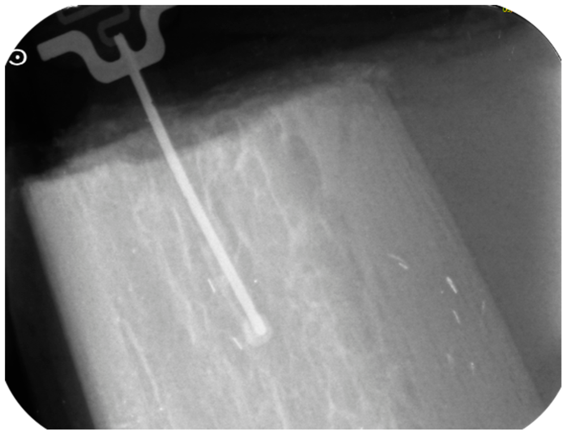
Figure 2.
Prototypes of the monophasic intraoperative probe. Each probe consists of a narrow shaft, which carries two copper electrodes at its tip and is inserted into the osteotomy, and a connector at the opposite end, embedded in a resin body for handling.
Figure 2.
Prototypes of the monophasic intraoperative probe. Each probe consists of a narrow shaft, which carries two copper electrodes at its tip and is inserted into the osteotomy, and a connector at the opposite end, embedded in a resin body for handling.
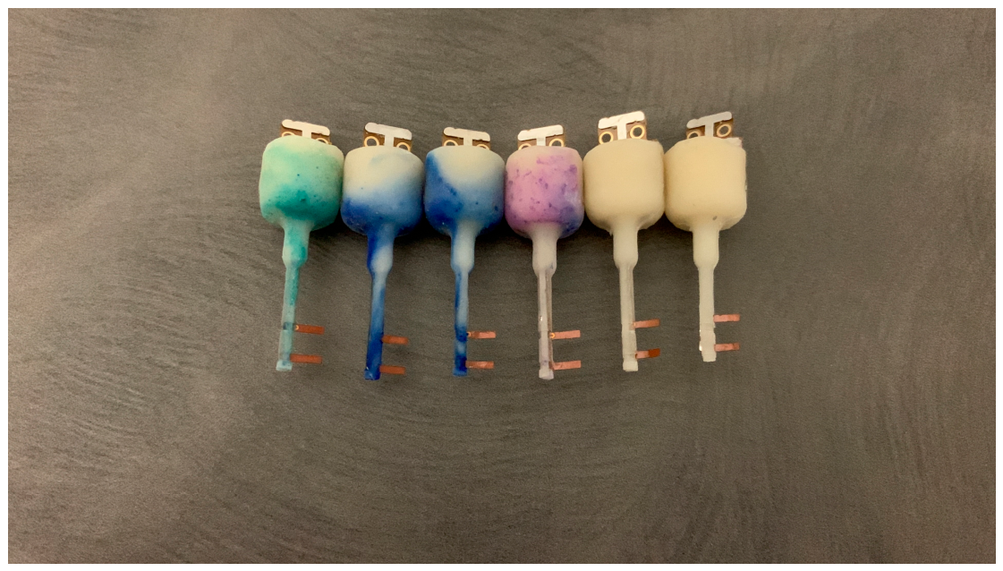
Figure 3.
Experimental set-up. The Quality-Bone unit (left) is connected to the probe mounted on the handpiece (far left) and, through a USB cable, to a laptop for real-time acquisition and storage of the impedance data (serial monitor on screen).
Figure 3.
Experimental set-up. The Quality-Bone unit (left) is connected to the probe mounted on the handpiece (far left) and, through a USB cable, to a laptop for real-time acquisition and storage of the impedance data (serial monitor on screen).
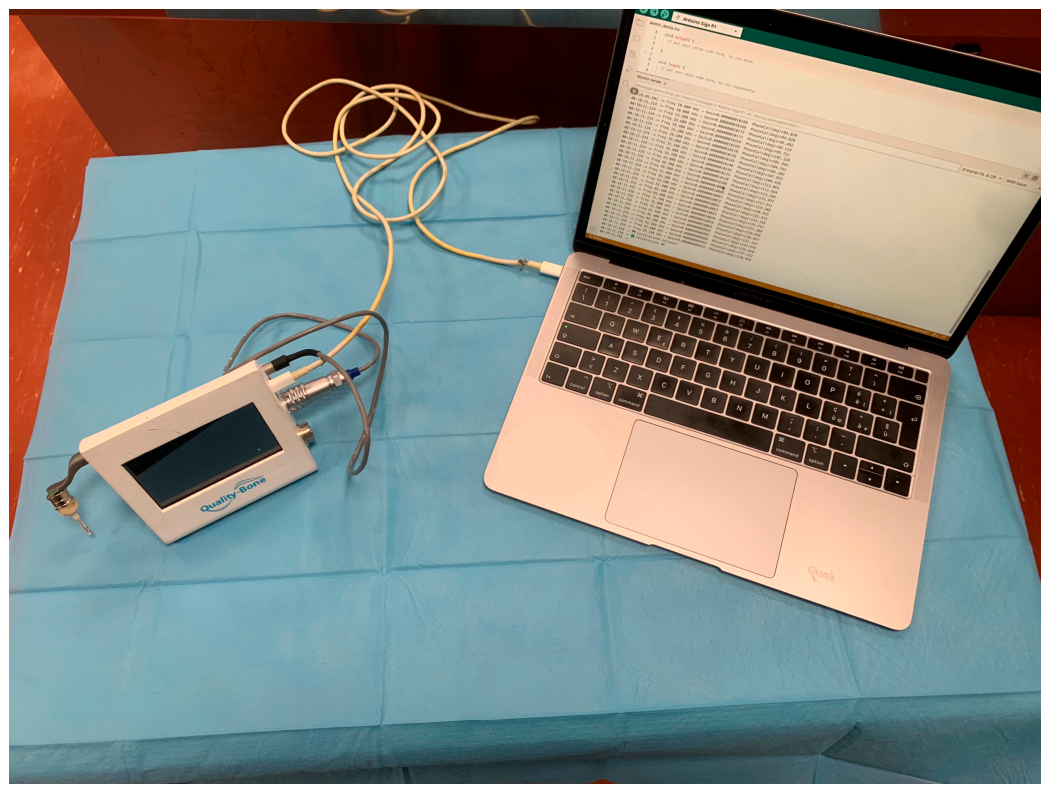
Figure 4.
Pearson correlation coefficient between log10|Z| and ISQ as a function of analysis frequency (n = 28). Correlation increases monotonically and reaches its maximum at 99.1 kHz.
Figure 4.
Pearson correlation coefficient between log10|Z| and ISQ as a function of analysis frequency (n = 28). Correlation increases monotonically and reaches its maximum at 99.1 kHz.
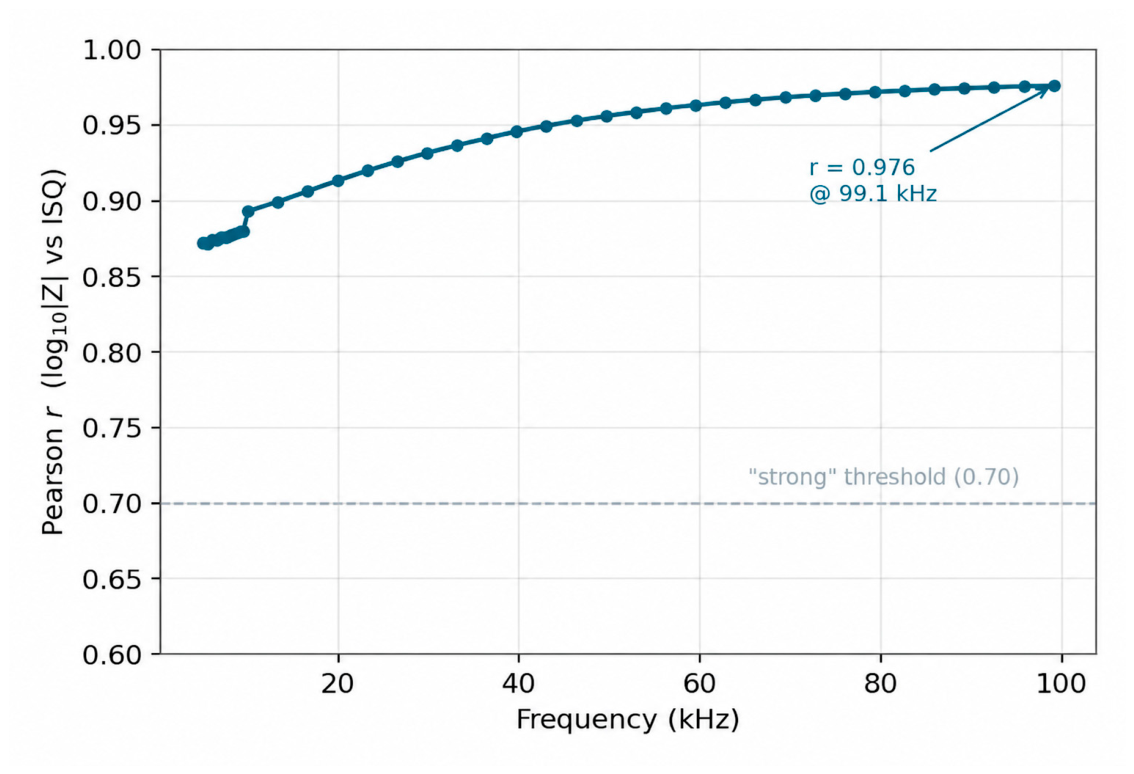
Figure 5.
Relationship between log10|Z| at 99.1 kHz and ISQ (n = 28), with regression line and 95% confidence band. The two excluded samples (no. 10 and 19) are shown in gray.
Figure 5.
Relationship between log10|Z| at 99.1 kHz and ISQ (n = 28), with regression line and 95% confidence band. The two excluded samples (no. 10 and 19) are shown in gray.
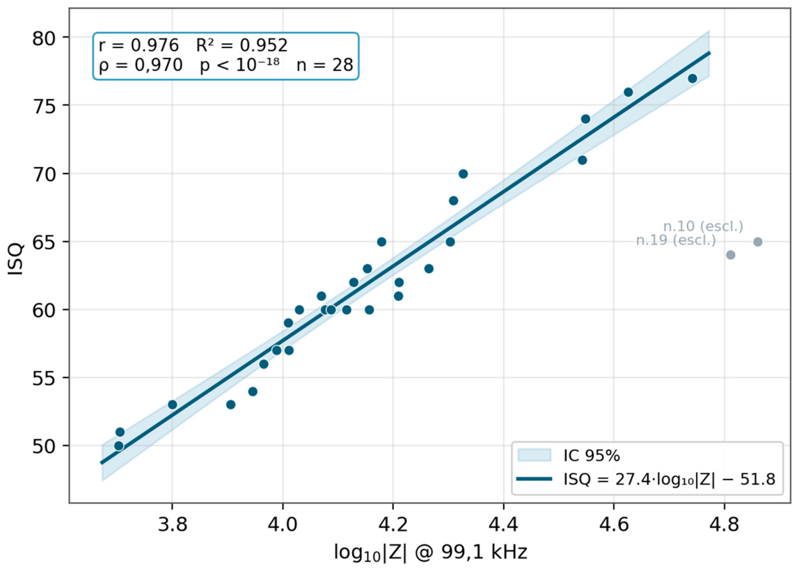
Figure 6.
Representative impedance spectra |Z|(f) for samples with low (no. 11, ISQ 50), medium (no. 30, ISQ 60), and high (no. 15, ISQ 77) ISQ.
Figure 6.
Representative impedance spectra |Z|(f) for samples with low (no. 11, ISQ 50), medium (no. 30, ISQ 60), and high (no. 15, ISQ 77) ISQ.
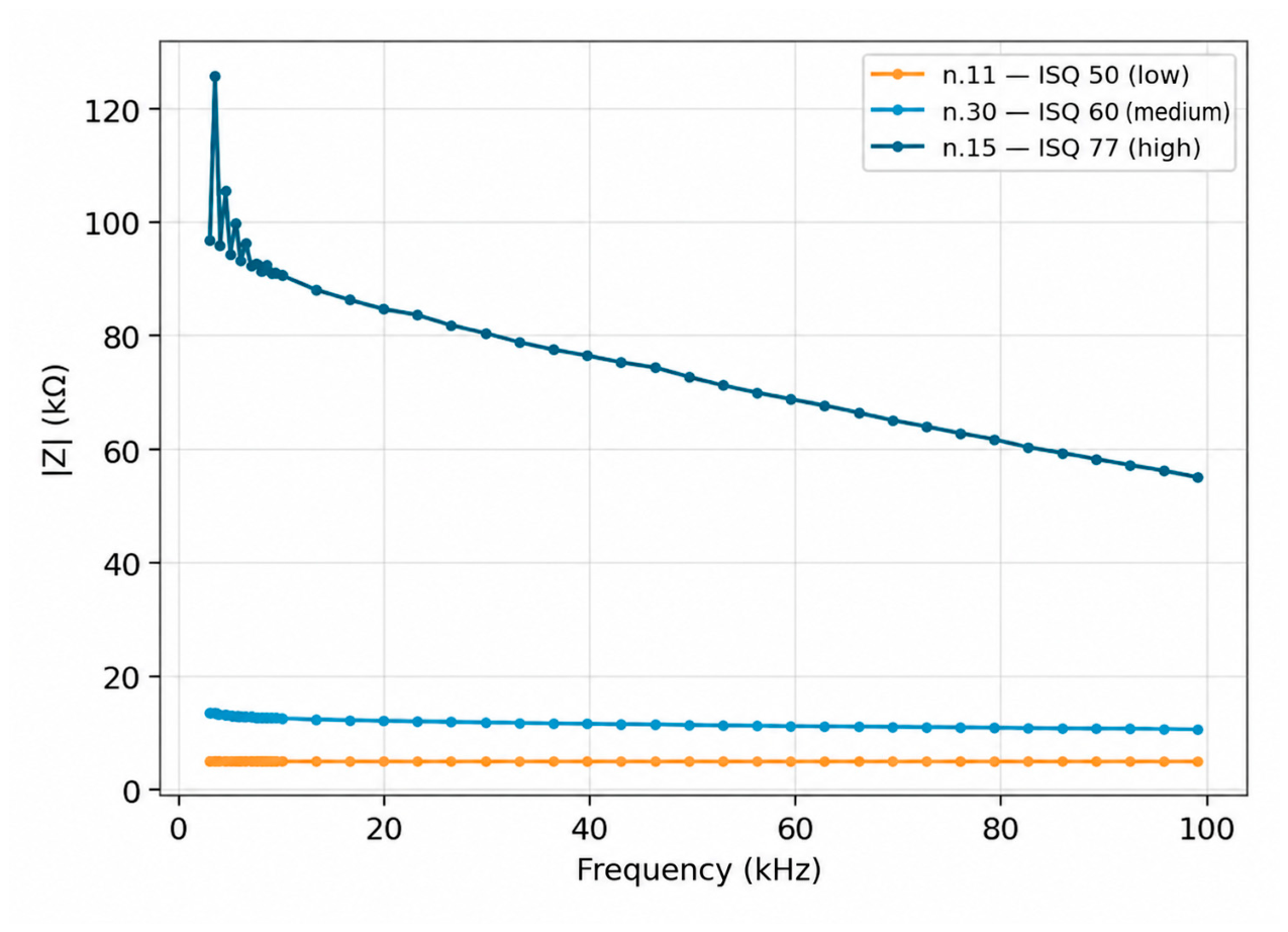

Table 1.
Descriptive statistics of the main variables (n = 28).
| Variable | Min / Max / Mean ± SD / Median (IQR) |
|---|---|
| ISQ | 50.0 / 77.0 / 61.7 ± 7.1 / 60.5 (57.0–65.0) |
| |Z| at 99.1 kHz (kΩ) | 5.0 / 55.2 / 16.8 ± 11.7 / 13.2 (10.1–18.8) |
| Phase at 99.1 kHz (°) | −51.9 / 4.4 / −17.8 ± 16.5 / −12.0 (−29.5 to −5.4) |
Table 2.
|Z|–ISQ correlation as a function of frequency (n = 28): Pearson coefficients (linear and logarithmic scale), Spearman’s ρ, and R2. The operating frequency of the QBP parameter (99.1 kHz) is highlighted. For logarithmic-scale coefficients, the 95% confidence interval (Fisher’s z-transformation) is given in parentheses. Estimates at different frequencies are derived from the same samples and are not independent.
Table 2.
|Z|–ISQ correlation as a function of frequency (n = 28): Pearson coefficients (linear and logarithmic scale), Spearman’s ρ, and R2. The operating frequency of the QBP parameter (99.1 kHz) is highlighted. For logarithmic-scale coefficients, the 95% confidence interval (Fisher’s z-transformation) is given in parentheses. Estimates at different frequencies are derived from the same samples and are not independent.
| Frequency | Pearson r | Spearman ρ | Linear R2 | Pearson r (log) | R2 (log) |
|---|---|---|---|---|---|
| 5.0 kHz | 0.80 | 0.87 | 0.64 | 0.87 (0.74–0.94) | 0.76 |
| 10.0 kHz | 0.82 | 0.92 | 0.67 | 0.89 (0.77–0.95) | 0.80 |
| 19.9 kHz | 0.85 | 0.94 | 0.72 | 0.91 (0.81–0.96) | 0.83 |
| 29.8 kHz | 0.87 | 0.95 | 0.75 | 0.93 (0.85–0.97) | 0.87 |
| 52.9 kHz | 0.89 | 0.95 | 0.80 | 0.96 (0.91–0.98) | 0.92 |
| 99.1 kHz | 0.92 | 0.97 | 0.84 | 0.98 (0.96–0.99) | 0.95 |
Disclaimer/Publisher’s Note: The statements, opinions and data contained in all publications are solely those of the individual author(s) and contributor(s) and not of MDPI and/or the editor(s). MDPI and/or the editor(s) disclaim responsibility for any injury to people or property resulting from any ideas, methods, instructions or products referred to in the content. |
© 2026 by the authors. Licensee MDPI, Basel, Switzerland. This article is an open access article distributed under the terms and conditions of the Creative Commons Attribution (CC BY) license (http://creativecommons.org/licenses/by/4.0/).
Copyright: This open access article is published under a Creative Commons CC BY 4.0 license, which permit the free download, distribution, and reuse, provided that the author and preprint are cited in any reuse.