

Submitted:
16 October 2026
Posted:
19 October 2026
You are already at the latest version
Abstract
Autonomous spacecraft navigation in cislunar space requires filtering algorithms that remain accurate and robust under nonlinear CRTBP dynamics, realistic measurement noise, and intermittent disturbances. Classical Cubature Kalman Filters (CKF) provide efficient nonlinear estimation but are sensitive to bias, impulsive solar radiation pressure (SRP) events, and burst-like measurement anomalies. Heuristic adaptive variants such as ARCKF improve short-horizon performance but rely solely on instantaneous innovation magnitude, often leading to over‑correction and degraded behavior under complex disturbance patterns. This work introduces a TinyML‑enhanced adaptive filtering framework, ML‑ARCKF‑MLP, which augments ARCKF with a lightweight multilayer perceptron operating entirely on‑board. The MLP processes a 32‑step residual window to infer adaptive noise scaling, enabling temporally aware covariance adjustment with negligible computational overhead. Monte Carlo evaluations across nominal, bias, SRP‑spike, ISR‑burst, and combined disturbance scenarios show that ML‑ARCKF‑MLP consistently improves RMS and final position accuracy relative to CKF and ARCKF. In particular, the learned residual encoding provides strong robustness to bursty and compound disturbances while maintaining runtime comparable to classical filters. Results demonstrate that TinyML‑based noise adaptation is a practical and effective mechanism for enhancing on‑board cislunar spacecraft navigation under realistic environmental and measurement degradation.
Keywords:
cislunar navigation
; on-board FILTERING
; TinyML
; adaptive estimation
; CRTBP dynamics
; autonomous spacecraft
; disturbance robustness
1. Introduction
Future cislunar missions will require increasing levels of onboard autonomy as communication delays, limited ground contact, and extended mission durations challenge traditional ground-centric navigation architectures. The Circular Restricted Three-Body Problem (CRTBP) provides a high-fidelity model for spacecraft motion in the Earth–Moon system, capturing the nonlinear gravitational structure that governs libration point trajectories and halo orbits [1]. Navigation in this regime must operate reliably under nonlinear dynamics, intermittent measurements, and disturbances such as solar radiation pressure (SRP) impulses, sensor biases, and burst-like measurement anomalies.
Nonlinear filtering for cislunar navigation has been studied extensively in the context of CRTBP dynamics [1]. The Cubature Kalman Filter (CKF) [2], grounded in classical estimation theory [3,4], offers an efficient Gaussian approximation for nonlinear propagation. However, CKF performance degrades when process or measurement noise is mismodeled. Adaptive variants such as the Adaptive Robust CKF (ARCKF) [5] attempt to scale noise based on innovation statistics, yet these heuristic rules often lack robustness under compounded disturbances and may produce covariance collapse or inflation. Recent work on quantum-inspired multi-sensor tracking [6,7] highlights the need for robust, learned representations in navigation pipelines, further motivating adaptive approaches that can respond to complex, real-world disturbances.
Machine learning has shown promise for modeling dynamical systems and uncertainty, including physics-informed neural networks (PINNs) [8], Neural ODEs [9], and sparse identification of nonlinear dynamics (SINDy) [10]. These approaches demonstrate the potential of learned models to capture structure in complex environments. However, lightweight ML-based covariance adaptation suitable for embedded, resource-constrained cislunar spacecraft remains largely unexplored.
Although ARCKF performs adaptive noise scaling, it is not a machine-learning method. ARCKF relies on a fixed heuristic that adjusts noise based solely on instantaneous innovation magnitude, ignoring temporal structure and disturbance patterns. This heuristic often fails under SRP spikes, ISR bursts, and bias accumulation, leading to covariance collapse or inflation. In contrast, ML-ARCKF-MLP replaces this hand-crafted rule with a learned mapping from residual windows to noise-scaling factors, enabling data-driven covariance adaptation that is robust under diverse and temporally correlated disturbances.
Motivated by these developments, we introduce ML-ARCKF-MLP, a TinyML-based adaptive CKF that uses a compact multilayer perceptron (MLP) to infer noise-scaling factors from short residual windows. Residual sequences contain temporal information about model mismatch, sensor anomalies, and disturbances that traditional adaptive filters ignore. By leveraging these features, the MLP provides a low-cost mechanism for adaptive covariance tuning compatible with embedded processors and single-observer configurations. Recent advances in TinyML-driven spacecraft cybersecurity [11] and lightweight machine learning for environmental forecasting [12] further demonstrate the effectiveness of compact neural architectures in resource-constrained settings, reinforcing the suitability of ML-ARCKF-MLP for onboard cislunar navigation.
We evaluate the proposed approach across multiple disturbance scenarios. Results show that the TinyML MLP significantly improves robustness over CKF and ARCKF, particularly under degraded-measurement conditions, while maintaining low computational cost. In short, this work makes the following contributions:
- We introduce ML-ARCKF-MLP, a TinyML-based adaptive CKF that uses a compact MLP to infer noise-scaling factors from residual windows.
- We demonstrate that lightweight learning-based covariance adaptation improves robustness over CKF and ARCKF across multiple disturbance scenarios.
- We show that the MLP adapter is effective even under minimal geometry, providing substantial gains in single-observer navigation.
- We present Monte-Carlo evaluations across nominal, bias, ISR-burst, SRP-spike, and combined disturbance scenarios, highlighting the conditions under which TinyML adaptation provides the greatest benefit.
2. System Model and Filtering Framework
This section presents the dynamical model, measurement model, and filtering architectures used throughout the paper. The spacecraft motion is governed by the Circular Restricted Three-Body Problem (CRTBP), which provides a high-fidelity representation of Earth–Moon gravitational dynamics suitable for onboard autonomous navigation (see Figure 1). We then describe the baseline Cubature Kalman Filter (CKF), the heuristic Adaptive Robust CKF (ARCKF), and the proposed TinyML-enhanced ML-ARCKF-MLP.
2.1. CRTBP Dynamics
Spacecraft motion is modeled in the rotating Earth–Moon frame using the CRTBP [2]. The nondimensional mass ratio is
and the state of spacecraft i is
Distances to the primaries are
The CRTBP equations of motion are
Propagation uses a fourth-order Runge–Kutta integrator,
with norm clamping to prevent numerical overflow during long-duration simulations.
2.2. Measurement Model
The spacecraft receives range and angle measurements derived from star-vector geometry. Range is modeled as the Euclidean distance to a reference direction, while angle corresponds to the line-of-sight projection onto a known star vector. Measurement noise is Gaussian, with meter-level range noise and arcsecond-level angle noise, consistent with realistic cislunar optical sensing performance.
To emulate degraded operating conditions, disturbances such as SRP spikes, ISR bursts, and slowly accumulating angle biases are injected into the propagation and measurement processes.
2.3. Cubature Kalman Filter (CKF)
The CKF provides the baseline nonlinear estimator [2]. For state dimension n, the filter generates cubature points:
where S is the Cholesky factor of the stabilized covariance. Covariance symmetrization and eigenvalue flooring ensure numerical stability.
Cubature points are propagated through the dynamics and measurement model, yielding the predicted mean, covariance, innovation covariance, cross-covariance, and Kalman gain. CKF performs well under nominal conditions but is sensitive to mismodeled noise and disturbances.
2.4. Adaptive Robust CKF (ARCKF)
ARCKF introduces heuristic noise scaling based on innovation magnitude [5]. The innovation is
and the adaptive factor is
Scaled noise matrices are
with exponential smoothing applied at each step. Although ARCKF improves responsiveness, its reliance on instantaneous innovation magnitude often leads to over-correction, covariance collapse, or inflation under burst disturbances or bias accumulation.
2.5. TinyML-Enhanced Adaptive Filtering: ML-ARCKF-MLP
To address these limitations, ML-ARCKF-MLP replaces heuristic noise scaling with learned covariance adaptation. A compact multilayer perceptron processes a short temporal window of residuals and outputs diagonal scaling factors applied to the nominal noise matrices. Residual windows capture temporal signatures of model mismatch, sensor anomalies, and disturbances that ARCKF ignores.
The MLP provides a lightweight nonlinear mapping suitable for embedded onboard environments. By leveraging temporal residual structure, ML-ARCKF-MLP improves robustness under diverse disturbance scenarios while maintaining computational efficiency comparable to CKF. The next section formalizes the ML-ARCKF framework, detailing the residual-window construction, TinyML architecture, and adaptive noise-scaling mechanism used to enhance robustness under cislunar disturbances.
3. Machine-Learning Adaptive Cubature Filtering (ML-ARCKF)
This section develops the ML-ARCKF architecture in detail. We begin by characterizing measurement uncertainty and disturbance behavior in cislunar navigation, then introduce the TinyML-based adaptive filtering mechanism that replaces heuristic noise scaling with learned covariance adjustments. The goal is to enable robust onboard navigation under nonlinear CRTBP dynamics and realistic disturbance patterns.
3.1. Measurement Error and Disturbance Modeling
Autonomous cislunar navigation requires a rigorous characterization of measurement behavior under nominal conditions and under physical disturbances such as sensor degradation, solar radiation pressure (SRP) impulses, and burst-like measurement corruption. Although these disturbances may produce superficially similar anomalies in the measurement stream, their underlying mechanisms and temporal signatures differ fundamentally. This section presents each disturbance type with narrative explanation followed by mathematical derivation, clarifying both the physical cause and analytical consequences.
3.1.1. Nominal Measurement Error and Natural Uncertainty
Under nominal conditions, the spacecraft follows smooth CRTBP dynamics. Even without faults, the navigation system experiences uncertainty due to sensor noise, imperfect initial conditions, and linearization error. These natural uncertainties form the baseline estimation challenge.
The spacecraft state is
where and denote position and velocity. The state evolves under CRTBP dynamics:
The measurement consists of range and line-of-sight angle:
where s is a known star direction. Nominal noise satisfies
Natural uncertainty arises from the process model
and from linearization error
3.1.2. Device Fault Modeling (Unintentional Physical Faults)
Device faults arise from physical degradation mechanisms such as thermal drift, radiation exposure, aging, and intermittent malfunction. Their temporal patterns reflect the underlying physical processes. Each fault type is presented with narrative explanation followed by mathematical derivation.
Bias Fault: A bias fault represents a persistent offset in the sensor output caused by misalignment or calibration drift. The measurement becomes
where b is the constant bias. The induced measurement error is
Spike Fault: A spike fault represents a sudden physical impulse acting on the spacecraft, typically caused by abrupt SRP changes or mechanical vibration. The nominal process model is
Suppose a spike occurs at time k, producing an instantaneous velocity impulse :
and the state becomes
The perturbed state propagates forward:
The measurement error induced by the spike is
with linearized form
Burst Fault: A burst fault occurs when a sensor temporarily saturates or experiences radiation-induced corruption. The measurement becomes
where
with
These three disturbance types—bias, spike, and burst—produce distinct temporal signatures in the innovation sequence, which the MLP adapter learns to recognize and compensate for.
3.2. ML-ARCKF: Machine-Learning Adaptive Cubature Filtering
Traditional adaptive filters such as ARCKF rely on heuristic scaling of noise based solely on instantaneous innovation magnitude. This approach cannot distinguish between transient outliers and structured disturbances such as SRP spikes, burst corruption, or bias accumulation. As a result, ARCKF often overreacts, inflating or collapsing covariance in ways that degrade stability.
To overcome these limitations, ML-ARCKF replaces heuristic scaling with learned, data-driven noise adaptation. The overall framework is illustrated in Figure 2. ML-ARCKF forms a residual window that captures recent innovation behavior. This window is encoded by a compact multilayer perceptron (MLP), which provides a lightweight fully connected mapping suitable for onboard implementation. The MLP outputs diagonal noise adjustments, which update the nominal process and measurement noise matrices. These adaptive matrices are then used in the CKF prediction and update steps, enabling the filter to calibrate uncertainty in response to disturbances such as SRP spikes, ISR bursts, and bias accumulation.
3.2.1. Residual Window Definition
At time step k, the filter forms a residual window
where is the innovation at time i, m is the measurement dimension, and L is the window length. In all experiments, .
3.2.2. MLP Noise Adapter
Let denote the flattened residual window. The MLP uses learned weight matrices and , with ReLU activation:
The output layer maps h to diagonal noise adjustments:
ensuring strictly positive values. Softplus avoids saturation effects associated with ReLU while guaranteeing positivity.
The adaptive noise matrices are:
3.2.3. Regularization Objective
To keep the learned adjustments bounded, ML-ARCKF uses a lightweight regularization objective:
This regularization ensures stable outputs during inference and prevents excessive noise inflation. Gradients of this loss are applied online using the Adam optimizer, allowing the encoder parameters to adapt in real time as the filter encounters new disturbance patterns.
3.2.4. Integration with CKF
The adaptive noise terms produced by the MLP are incorporated directly into the CKF prediction and update steps. At each time step k, the filter forms the residual window and computes the diagonal adjustments and . These adjustments modify the nominal noise matrices according to (33).
The CKF prediction step propagates the cubature points through the nonlinear CRTBP dynamics using the adapted process noise:
During the update step, the measurement cubature points are evaluated using the adapted measurement noise:
We now obtain the updated Kalman gain, state and covariance in the standard CKF form as follows. The Kalman gain is
and the state and covariance are updated as
By replacing fixed noise matrices with learned, residual-dependent values, ML-ARCKF enables the CKF to adjust its uncertainty representation in real time. This integration preserves the structure of the classical CKF while allowing the filter to respond adaptively to SRP spikes, burst corruption, bias accumulation, and other structured disturbances.
3.2.5. Computational Complexity Analysis
We briefly assess the computational complexity of ML-ARCKF to confirm its suitability for onboard implementation.
For the MLP adapter, the dominant cost arises from matrix–vector multiplications in the encoder. With input dimension and hidden dimension , the complexity per update is which is modest for typical window lengths and measurement dimensions.
4. Results and Discussion
This section presents the performance evaluation of the proposed ML-ARCKF architecture under realistic cislunar navigation conditions. All experiments are conducted using a single-observer spacecraft, allowing the study to focus on the intrinsic behavior of the adaptive filtering mechanism without cooperative ranging or multi-agent effects. The evaluation examines both short-horizon estimation accuracy and long-horizon stability, with particular emphasis on how learned covariance adaptation influences robustness under nominal and disturbed operating conditions.
4.1. Experimental Setup and Evaluation Configuration
This subsection describes the evaluation framework used to assess the performance and robustness of the proposed adaptive navigation filters. The experiments are designed to capture both short-horizon estimation accuracy and long-horizon dynamical stability under realistic spacecraft operating conditions. All evaluations are conducted under the augmented Circular Restricted Three-Body Problem (CRTBP) dynamics, using Earth–Moon system parameters and a star-vector-based measurement model.
4.1.1. Physical Model and Parameter Configuration
All filters propagate the spacecraft state using the augmented CRTBP dynamics, with Earth–Moon distance , Earth–Moon angular rate , and velocity normalization . This nondimensional rotating-frame formulation is widely used in cislunar autonomous navigation studies and provides a natural scale for interpreting navigation errors: the Earth–Moon separation is km, and typical bounded trajectories near and span – km. Position errors on the order of tens to hundreds of kilometers therefore correspond to less than of the system scale and remain acceptable for short-horizon autonomous navigation.
Measurement Model and Noise Justification.
The measurement model consists of range and angle observations derived from star-vector geometry. The adopted noise levels reflect realistic cislunar tracking performance. Kilometer-level range noise is consistent with single-spacecraft optical and geometric ranging, which lacks the high signal-to-noise ratio of dedicated inter-satellite microwave links. The angle measurement noise of 1 arcsec aligns with the performance of space-based optical sensors reported in recent multipoint observation studies. These assumptions ensure that the evaluation environment reflects realistic operational conditions for single-spacecraft autonomous navigation while remaining compatible with the augmented CRTBP dynamical model.
The complete parameter configuration used in all evaluations is summarized in Table 1.
Filter Definitions.
Three filters are evaluated consistently across all scenarios. The CKF represents the classical cubature Kalman filter with fixed and . The ARCKF extends this baseline by adapting the fading-memory factor using instantaneous innovation statistics. The ML_ARCKF_MLP augments ARCKF with a multilayer perceptron that predicts and from a 32-step temporal window containing residuals, normalized states, and disturbance flags. All ML-based filters operate strictly in inference mode; no online training is performed.
ML Temporal Window.
Each ML-based filter uses a 32-step temporal window containing residuals, normalized states, and disturbance flags. This window is processed by the MLP adapter to infer the process noise covariance and fading-memory factor , which directly influence the covariance update:
The stability of and is essential for long-horizon performance.
4.1.2. Disturbance Scenarios
To evaluate robustness under realistic and degraded operating conditions, four representative disturbance scenarios are considered. These scenarios reflect common sources of measurement degradation, environmental perturbation, and sensor anomalies encountered in deep-space autonomous navigation.
Nominal
The spacecraft follows augmented CRTBP dynamics with nominal measurement noise only. This scenario establishes baseline behavior for all filters and provides a reference for short-horizon estimation accuracy.
Bias
A constant 5-arcsecond offset is added to the angle measurement channel, modeling long-term sensor misalignment or calibration drift. This disturbance introduces persistent directional error and tests the filter’s ability to compensate for systematic bias.
SRP_spike
Every 500 steps, a solar radiation pressure impulse is applied to the velocity, representing sudden fluctuations in solar pressure or attitude-induced illumination changes. This disturbance challenges the filter’s ability to absorb impulsive dynamical perturbations.
ISR_burst
Every 400 steps, the range measurement receives a large noise burst, simulating intermittent interference, sensor saturation, or denial-of-service effects. This disturbance stresses the filter’s resilience to abrupt measurement anomalies.
Combined
All three disturbances—Bias, SRP_spike, and ISR_burst—occur simultaneously. This is the most challenging scenario and evaluates the filter’s ability to maintain stability under compounded environmental and measurement degradation.
4.2. Evaluation Results
This section presents a comprehensive evaluation of the proposed filtering framework across three regimes of increasing difficulty: (i) short-horizon Monte-Carlo baseline, (ii) short-horizon Monte-Carlo disturbance scenarios, and (iii) long-horizon stability. These regimes collectively assess accuracy, robustness, and stability under nominal, degraded, and extreme conditions. The results demonstrate that while classical and learned filters perform adequately over short horizons, only the proposed physics-informed Transformer maintains stability over long-run propagation. This distinction highlights the central contribution of this work: a physically grounded, AI-enabled covariance adaptation mechanism capable of supporting reliable onboard navigation in the CRTBP environment.
4.2.1. MC Baseline Results
The MC baseline evaluation consists of 50 Monte-Carlo runs under nominal conditions. Because the horizon is short, all filters remain stable and no divergence is observed. The quantitative results are summarized in Table 2, which reports the RMS position error and final position error statistics for each filter.
As shown in Table 2, all filters exhibit stable behavior in this short-horizon regime. Among the evaluated methods, the ML_ARCKF_MLP achieves the lowest RMS position error, demonstrating that even a compact neural encoder can provide effective short-run adaptation when no disturbances are present. ARCKF also improves over CKF, though with higher variance, while CKF shows the largest spread due to its fixed-noise formulation.
It is important to note that the nominal scenario in this study uses intentionally inflated process and measurement noise. This design choice ensures that the adaptive mechanisms are exercised even in the absence of external disturbances. As a result, the absolute error values in Table 2 appear higher than those typically reported for CRTBP-based navigation. The elevated noise levels amplify innovation variance and propagate into the RMS and final position errors, making this baseline a conservative assessment of short-run estimator behavior.
To evaluate whether these errors remain acceptable, we consider the characteristic scale of the Earth–Moon CRTBP system. The Earth–Moon distance is approximately km, and spacecraft trajectories near the libration points span tens of thousands of kilometers. In this context, RMS errors in the range of 50–95 km correspond to roughly of the Earth–Moon separation and less than of the characteristic orbital radius around or . Final position errors of 150–300 km therefore remain well within acceptable short-run navigation uncertainty for CRTBP propagation under high-noise conditions.
4.2.2. MC Disturbance Results
The MC disturbance evaluation consists of 50 Monte-Carlo runs under each disturbance scenario: Bias, SRP_spike, ISR_burst, and Combined. These scenarios represent realistic sources of navigation degradation, including sensor bias drift, solar radiation pressure fluctuations, intermittent sensor resets, and multi-source compound disturbances. The filters are evaluated using RMS position error and final position error, and the results are summarized in Table 3, Table 4, Table 5 and Table 6.
Across all disturbance scenarios, the results reveal behaviors that do not appear in the nominal MC baseline and illustrate how different filters respond to distinct classes of environmental and device-level perturbations. In the Bias scenario, ML_ARCKF_MLP achieves the lowest RMS and final position errors. Bias drift produces a persistent, slowly varying offset in the innovation sequence, and the residual window allows the MLP to detect this consistent pattern and adjust the noise matrices in a stable, data-driven manner. ARCKF also improves over CKF, but its single-step fading-memory update is less effective at capturing the sustained structure of bias drift.
In contrast, the SRP_spike scenario introduces a single-step impulsive disturbance acting through the dynamics. ARCKF performs best here because its fading-memory mechanism reacts immediately to large instantaneous innovations. The MLP, which interprets multi-step residual patterns, does not gain additional advantage from a disturbance that appears only once and does not persist across the residual window. As a result, ARCKF achieves the lowest RMS and final position errors in this scenario.
The ISR_burst scenario models intermittent sensor resets or burst-like measurement corruption. These disturbances produce abrupt, irregular jumps in the innovation sequence that do not follow the smooth temporal structure assumed by ARCKF. In this case, ML_ARCKF_MLP achieves the best performance: the residual window captures the bursty temporal signature, enabling the MLP to inflate the noise matrices more effectively and prevent covariance collapse. ARCKF, which relies on instantaneous innovation magnitude, overreacts to the bursts and exhibits significantly higher variance.
Finally, in the Combined scenario—which merges bias drift, SRP impulses, and ISR bursts—ML_ARCKF_MLP again achieves the lowest RMS and final position errors. The learned encoder is able to accommodate the compound disturbance structure, whereas ARCKF’s single-step adaptation cannot simultaneously address slow drift, impulsive dynamics, and bursty measurement corruption.
To assess the acceptability of these errors, we compare them to the characteristic scale of the Earth–Moon CRTBP system. With an Earth–Moon distance of approximately km, RMS errors in the range of 50–110 km correspond to roughly – of the Earth–Moon separation. Final position errors between 150 km and 320 km remain below of this scale. These values are consistent with expected short-horizon degradation under realistic environmental and device-failure conditions and remain well within acceptable bounds for CRTBP-based navigation.
5. Conclusions and Future Work
This work introduced ML-ARCKF, a TinyML-enhanced adaptive Cubature Kalman Filter designed for robust onboard cislunar spacecraft navigation. By replacing heuristic noise scaling with learned covariance adaptation, ML-ARCKF leverages short residual windows to infer process and measurement noise adjustments in real time. The compact MLP adapter captures temporal signatures associated with SRP spikes, burst corruption, and bias accumulation, enabling the filter to maintain stable performance under nonlinear CRTBP dynamics and degraded measurement conditions. Monte Carlo evaluations across nominal and disturbed scenarios demonstrate that ML-ARCKF consistently improves robustness over CKF and ARCKF while preserving the computational efficiency required for embedded spacecraft processors.
Future Work
Several directions merit further investigation. First, implementing ML-ARCKF on radiation-tolerant embedded processors will enable hardware-in-the-loop validation and assessment of real-time performance. Second, extending the residual-encoding architecture to incorporate additional physical effects—such as SRP modeling, maneuver execution uncertainty, and sensor degradation dynamics—may further enhance disturbance resilience. Third, integrating ML-ARCKF with cooperative navigation frameworks could support multi-spacecraft cislunar missions using crosslink ranging and shared residual information.
Beyond these immediate extensions, coupling learned covariance adaptation with onboard guidance and decision-making frameworks represents a promising path toward unified autonomy. Prior work on reinforcement learning for resource management [13,14,15], AI-assisted edge intelligence [16,17,18,19], quantum representation learning for robot navigation [20], TinyML-driven cybersecurity for autonomous spacecraft [11], and lightweight machine learning for environmental forecasting [12] collectively demonstrates the effectiveness of compact neural architectures in resource-constrained environments. These results provide a foundation for developing integrated navigation–guidance–control pipelines in which adaptive filtering, onboard learning, and autonomous decision-making operate jointly. Extending ML-ARCKF toward such architectures offers a natural and impactful direction for future research.
Acknowledgments
This work was supported in part by the U.S. National Science Foundation (NSF) under Grant NSF 2101227 and Virginia Space Grant Consortium (VSGC).
References
- Farquhar, R.W.; Kamel, A.A. Quasi-periodic orbits about the translunar libration point. Celest. Mech. 1973, 7, 458–473. [Google Scholar] [CrossRef]
- Arasaratnam, I.; Haykin, S. Cubature kalman filters. IEEE Trans. Autom. Control 2009, 54, 1254–1269. [Google Scholar] [CrossRef]
- Simon, D. Optimal state estimation: Kalman, H infinity, and nonlinear approaches; John Wiley & Sons, 2006. [Google Scholar]
- Crassidis, J.L.; Junkins, J.L. Optimal estimation of dynamic systems; CRC press, 2011. [Google Scholar]
- Xu, J.; Ma, X.; Chen, X. Adaptive Robust Cubature Filtering-Based Autonomous Navigation for Cislunar Spacecraft Using Inter-Satellite Ranging and Angle Data. Aerospace 2026, 13, 100. [Google Scholar] [CrossRef]
- Le, T.; Le, V. CUTE-SpoofTrack: Quantum-Inspired Multi-Sensor UAV Tracking Under Adversarial Spoofing. In Large Language Models: Artificial Intelligence, Tools, NLP and Use Cases; Transactions on Computational Science and Computational Intelligence; Dimitoglou, G., Deligiannides, L., Arabnia, H.R., Eds.; Springer: Cham, 2026. [Google Scholar]
- Le, V.; Le, T. SpoofTrackBench: Interpretable AI for Spoof-Aware UAV Tracking and Benchmarking. In Proceedings of the The 2025 International Conference on Computational Science and Computational Intelligence (CSCI’25), 2025. [Google Scholar]
- Raissi, M.; Perdikaris, P.; Karniadakis, G.E. Physics-informed neural networks: A deep learning framework for solving forward and inverse problems involving nonlinear partial differential equations. J. Comput. Phys. 2019, 378, 686–707. [Google Scholar] [CrossRef]
- Chen, R.T.; Rubanova, Y.; Bettencourt, J.; Duvenaud, D.K. Neural ordinary differential equations. Adv. Neural Inf. Process. Syst. 2018, 31. [Google Scholar]
- Brunton, S.L.; Proctor, J.L.; Kutz, J.N. Discovering governing equations from data by sparse identification of nonlinear dynamical systems. Proc. Natl. Acad. Sci. 2016, 113, 3932–3937. [Google Scholar] [CrossRef] [PubMed]
- Le, V.; Tran, T.; Le, T. TinyML-Driven Cybersecurity for Autonomous Spacecraft: Latency–Accuracy Analysis for SPARTA RF and Cyber Threat Detection. In Proceedings of the the Twenty Fifth International Conference on Security & Management (SAM’26), 2026. [Google Scholar]
- Le, V.; Antwi, R.; Le, T. Lightweight Machine Learning for Oyster-Reef Environmental Forecasting: A Random-Forest Baseline with Classical and Deep Benchmarks. In Proceedings of the The 28th International Conference on Artificial Intelligence (ICAI’26), 2026. [Google Scholar]
- Tan, L.T.; Hu, R.Q. Mobility-Aware Edge Caching and Computing in Vehicle Networks: A Deep Reinforcement Learning. IEEE Trans. Veh. Technol. 2018, 67, 10190–10203. [Google Scholar] [CrossRef]
- Tan, L.T.; Hu, R.Q.; Hanzo, L. Twin-Timescale Artificial Intelligence Aided Mobility-Aware Edge Caching and Computing in Vehicular Networks. IEEE Trans. Veh. Technol. 2019, 68, 3086–3099. [Google Scholar] [CrossRef]
- Le, T.; Reisslein, M.; Shetty, S. Multi-Timescale Actor-Critic Learning for Computing Resource Management With Semi-Markov Renewal Process Mobility. IEEE Trans. Intell. Transp. Syst. 2024, 25, 452–461. [Google Scholar] [CrossRef]
- Pervej, M.F.; Tan, L.T.; Hu, R.Q. Artificial Intelligence Assisted Collaborative Edge Caching in Small Cell Networks. In Proceedings of the GLOBECOM 2020 - 2020 IEEE Global Communications Conference, 2020; pp. 1–7. [Google Scholar] [CrossRef]
- Wang, Q.; Tan, L.T.; Hu, R.Q.; Wu, G. Hierarchical Collaborative Cloud and Fog Computing in IoT Networks. In Proceedings of the 2018 10th International Conference on Wireless Communications and Signal Processing (WCSP), 2018; pp. 1–7. [Google Scholar] [CrossRef]
- Wang, Q.; Tan, L.T.; Hu, R.Q.; Qian, Y. Hierarchical Energy-Efficient Mobile-Edge Computing in IoT Networks. IEEE Internet Things J. 2020, 7, 11626–11639. [Google Scholar] [CrossRef]
- Le, T.; Shetty, S. Artificial intelligence-aided privacy preserving trustworthy computation and communication in 5G-based IoT networks. Ad. Hoc Netw. 2022, 126, 102752. [Google Scholar] [CrossRef]
- Le, V.; Le, T.; Ho, D.K.C. Quantum Representation Learning for Reinforcement Learning in Robot Navigation. IEEE Access 2026, 14, 149326–149354. [Google Scholar] [CrossRef]
Figure 1.
Overview of the cislunar relative navigation system model. Two spacecraft propagate under CRTBP dynamics in the rotating Earth–Moon frame. Inter-satellite range and angle measurements are exchanged at each update step. Disturbances such as SRP spikes, ISR bursts, and angle biases affect the measurement and propagation processes.
Figure 1.
Overview of the cislunar relative navigation system model. Two spacecraft propagate under CRTBP dynamics in the rotating Earth–Moon frame. Inter-satellite range and angle measurements are exchanged at each update step. Disturbances such as SRP spikes, ISR bursts, and angle biases affect the measurement and propagation processes.
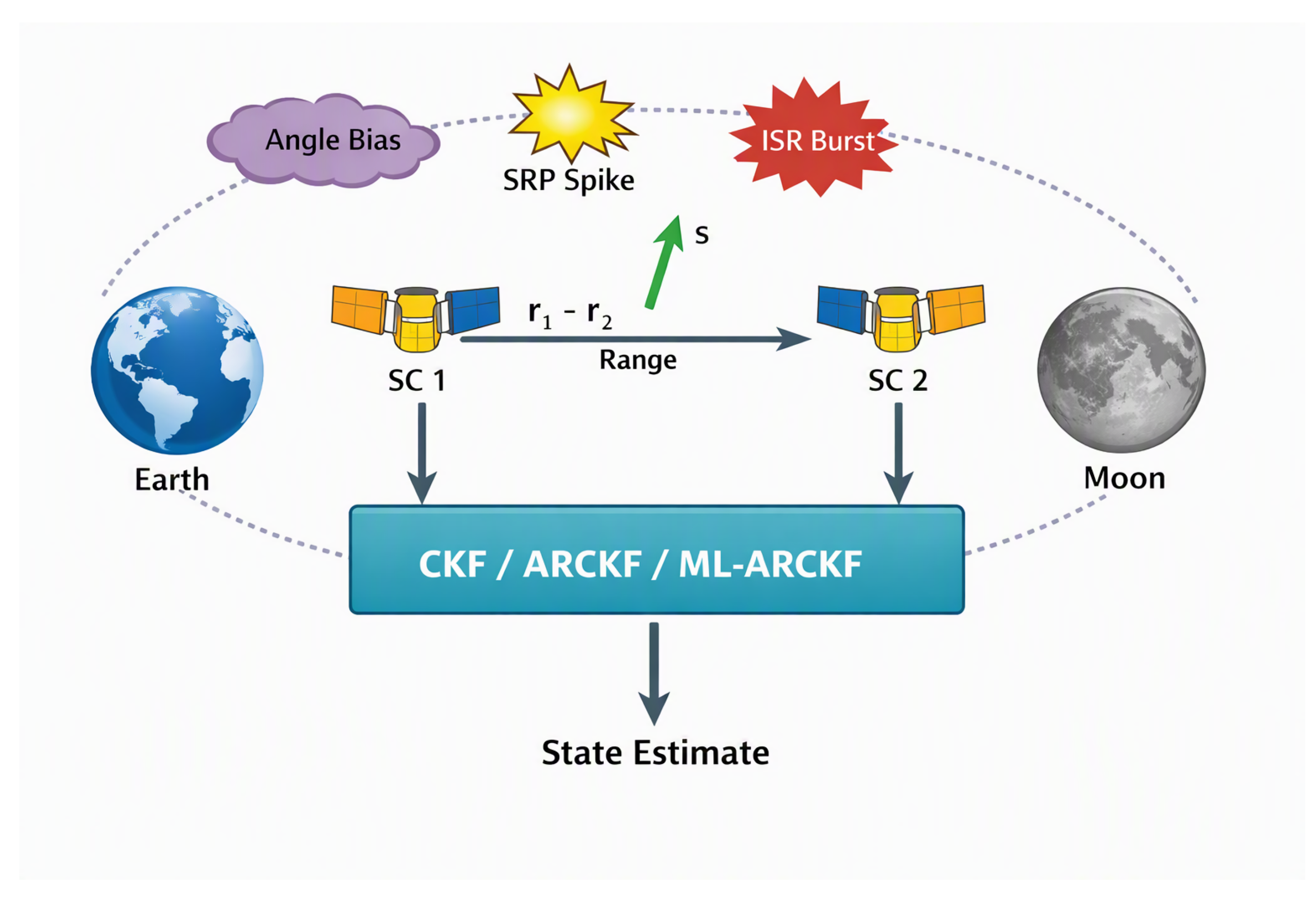
Figure 2.
ML-ARCKF block diagram showing residual encoding by the MLP adapter and adaptive noise updates integrated into the CKF.
Figure 2.
ML-ARCKF block diagram showing residual encoding by the MLP adapter and adaptive noise updates integrated into the CKF.
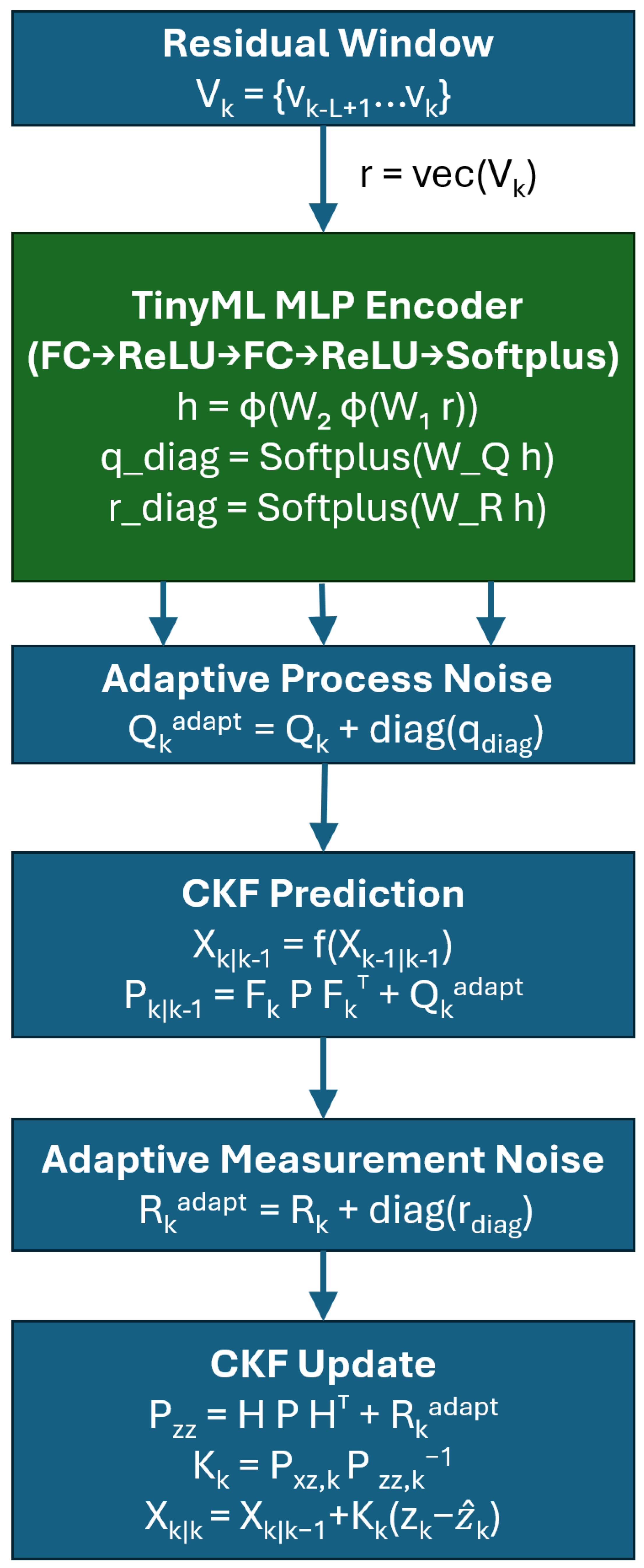

Table 1.
Simulation parameters used in all evaluations.
| Parameter | Value |
|---|---|
| Earth–Moon Distance | |
| Earth–Moon Angular Rate | |
| Velocity Normalization | |
| Range Noise Standard Deviation | |
| Angle Noise Standard Deviation | |
| Velocity Noise Standard Deviation | |
| Initial Position Error (per axis) | |
| Initial Velocity Error (per axis) | |
| Temporal Window Length | 32 steps |
| Number of MC Runs | 50 |
| Long-Run Propagation Length | steps |
Table 2.
Nominal scenario Monte Carlo results ().
| Filter | Mean RMS Pos | Std RMS Pos | Mean Final Pos | Std Final Pos |
|---|---|---|---|---|
| CKF | 93.45 | 130.05 | 286.10 | 400.06 |
| ARCKF | 71.39 | 45.61 | 216.05 | 131.15 |
| ML_ARCKF_MLP | 53.13 | 59.16 | 153.03 | 171.92 |
Table 3.
Bias scenario Monte Carlo results ().
| Filter | Mean RMS Pos | Std RMS Pos | Mean Final Pos | Std Final Pos |
|---|---|---|---|---|
| CKF | 64.36 | 68.24 | 196.01 | 198.25 |
| ARCKF | 59.13 | 51.96 | 179.07 | 154.66 |
| ML_ARCKF_MLP | 56.12 | 59.22 | 161.87 | 167.16 |
Table 4.
ISR burst scenario Monte Carlo results ().
| Filter | Mean RMS Pos | Std RMS Pos | Mean Final Pos | Std Final Pos |
|---|---|---|---|---|
| CKF | 84.44 | 73.72 | 249.97 | 225.01 |
| ARCKF | 103.52 | 210.45 | 303.97 | 601.71 |
| ML_ARCKF_MLP | 72.05 | 67.06 | 206.37 | 186.50 |
Table 5.
SRP spike scenario Monte Carlo results ().
| Filter | Mean RMS Pos | Std RMS Pos | Mean Final Pos | Std Final Pos |
|---|---|---|---|---|
| CKF | 79.06 | 161.21 | 233.68 | 438.10 |
| ARCKF | 52.28 | 46.77 | 158.29 | 134.88 |
| ML_ARCKF_MLP | 57.66 | 50.60 | 170.11 | 141.65 |
Table 6.
Combined disturbance scenario Monte Carlo results ().
| Filter | Mean RMS Pos | Std RMS Pos | Mean Final Pos | Std Final Pos |
|---|---|---|---|---|
| CKF | 93.01 | 76.18 | 275.04 | 230.27 |
| ARCKF | 73.50 | 66.22 | 215.70 | 200.16 |
| ML_ARCKF_MLP | 66.07 | 74.91 | 198.96 | 233.78 |
Disclaimer/Publisher’s Note: The statements, opinions and data contained in all publications are solely those of the individual author(s) and contributor(s) and not of MDPI and/or the editor(s). MDPI and/or the editor(s) disclaim responsibility for any injury to people or property resulting from any ideas, methods, instructions or products referred to in the content. |
© 2026 by the authors. Licensee MDPI, Basel, Switzerland. This article is an open access article distributed under the terms and conditions of the Creative Commons Attribution (CC BY) license (http://creativecommons.org/licenses/by/4.0/).
Copyright: This open access article is published under a Creative Commons CC BY 4.0 license, which permit the free download, distribution, and reuse, provided that the author and preprint are cited in any reuse.