

Submitted:
14 October 2026
Posted:
15 October 2026
You are already at the latest version
Abstract
Reliable and interpretable heart disease prediction across heterogeneous clinical cohorts remains a major barrier to clinical translation. This study presents an explainable, genetic-algorithm (GA)-optimized performance-weighted soft-voting (PWSV) framework for binary heart disease prediction using 920 records from the Cleveland, Hungary, Switzerland, and VA Long Beach cohorts. After data harmonization, leakage-aware preprocessing, and feature engineering, 29 encoded predictors were retained. GA independently optimized random forest, extra trees, radial basis function support vector machine, and gradient boosting using five-fold cross-validation confined to the development data. Each model’s mean cross-validated weighted F1-score was normalized into its ensemble weight, keeping both hyperparameter selection and weight estimation independent of the test data. Two complementary evaluation protocols were used: a stratified 80:20 development–test split to assess predictive performance and leave-one-dataset-out (LODO) validation to quantify cross-cohort generalizability. On the untouched test set, PWSV achieved 95.65% accuracy; disease-class precision, recall, and F1-score of 94.34%, 98.04%, and 96.15%, respectively; and a 98.11% area under the receiver operating characteristic curve, outperforming all optimized constituent classifiers. LODO accuracy ranged from 82.15% to 90.64%, revealing cohort-dependent performance variation that a random split alone would not capture. SHAP and LIME provided complementary global and patient-level explanations, and their aggregated feature rankings showed significant agreement (Spearman’s ρ = 0.867, p < 0.001). Overall, the framework integrates leakage-aware optimization, performance-driven probability fusion, source-aware validation, and concordant explanations within a reproducible pipeline. These findings support its potential for clinical decision support, while prospective multicenter validation remains necessary before deployment.
Keywords:
ensemble learning
; explainable artificial intelligence
; genetic algorithms
; heart disease prediction
; soft voting
1. Introduction
Cardiovascular diseases (CVDs) remain among the most serious global health challenges and are a leading cause of mortality worldwide. According to the World Health Organization (WHO) estimates reported in [1], CVDs caused an estimated 19.8 million deaths in 2022, accounting for approximately 32% of all deaths globally; nearly 85% of these deaths were attributable to heart attacks and strokes. Beyond their substantial contribution to mortality, including premature death among middle-aged adults, CVDs impose a considerable burden through long-term disability and the associated loss of healthy life years. This burden increased nearly 1.4-fold, from 320 million disability-adjusted life years (DALYs) in 1990 to 437 million in 2023 [1]. Heart disease is associated with several common risk factors that are both common and some modifiable ones, which have been highlighted in Figure 1, such as hypertension, high cholesterol levels, diabetes, obesity, smoking, and lack of physical activity. It has therefore become imperative to support timely intervention and clinical management. Proactive assessment may facilitate the earlier recognition and management of cardiovascular disease in high-risk populations [2]. Recently, ML algorithms have been widely applied to heart disease prediction, which is attributed to their capability to examine clinical data and identify complex patterns, which in turn help in diagnosing heart diseases and assessing risks [3,4]. The growing need for reliable computer-aided heart-disease classification and clinical decision-support systems has made heart disease prediction a major area of healthcare research [5,6].
As clinical data become increasingly available, machine learning (ML) has emerged as a powerful approach for analyzing patient information and identifying patterns associated with heart disease and other clinical conditions [7]. Algorithms such as Logistic Regression (LR), Support Vector Machine (SVM), Random Forest (RF), Decision Tree (DT), and Extreme Gradient Boosting (XGBoost) have been widely applied because of their strong classification capabilities and potential to improve diagnostic performance [8]. Although ML models can achieve strong performance, a single classifier may not consistently provide the best results across different datasets and clinical settings. Different algorithms process clinical information differently, with some being more effective in certain settings. Therefore, hybrid and ensemble approaches have gained considerable popularity since they capitalize on the advantages of several models [3,9]. By leveraging the complementary strengths of different classifiers, these methods may improve predictive performance. Among these approaches, soft voting is a widely used ensemble strategy that combines the predicted class probabilities of multiple classifiers. Nevertheless, when it comes to healthcare applications, achieving high predictive accuracy alone is insufficient for clinical adoption. Clinical decision-support models need to be accurate as well as interpretable and transparent, enabling clinicians to understand the factors contributing to each prediction and assess whether the model’s reasoning is clinically plausible.
For this reason, Explainable Artificial Intelligence (XAI) has become an important component in contemporary heart disease prediction research. Methods such as Shapley Additive exPlanations (SHAP), and Local Interpretable Model-agnostic Explanations (LIME) help explain how clinical features contribute to model predications, thereby making the decision process more transparent to clinicals [10]. Although heart disease prediction has been extensively investigated [3,5,8,11], there is limited consideration for frameworks that optimize heterogeneous classifiers together, derive ensemble weights from the optimized cross-validated performance of theses classifiers, combine global and local explanations, and evaluate robustness among heterogeneous data sources.
To address this gap, this study proposes an explainable performance-weighted soft-voting framework for the binary classification of heart disease. Specifically, the hyperparameters of four heterogeneous base classifiers—RF, Extra Trees (ET), Support Vector Machine with a Radial Basis Function kernel (RBF-SVM), and Gradient Boosting (GB)—are first optimized using a genetic algorithm (GA). The optimized classifiers are subsequently integrated through a performance-weighted soft-voting scheme. Within each outer evaluation split, the voting weights are re-estimated by normalizing the mean inner-cross-validated weighted F1-scores obtained exclusively from that split’s training data. Finally, SHAP is employed to provide global and instance-level feature attributions and identify the most influential clinical features, whereas LIME provides complementary case-specific explanations. Predictive performance is evaluated using a stratified 80:20 holdout test and leave-one-dataset-out validation across the four source cohorts. Early and accurate heart disease prediction has the potential to support timely clinical decision-making and patient management [12].
However, the predictive performance of machine learning classifiers is highly sensitive to their hyperparameter settings, and default configurations may not yield optimal results. Hyperparameter optimization is therefore important for identifying configurations that more effectively capture patterns in clinical data. Among the available optimization strategies, genetic algorithms (GAs) provide an effective mechanism for exploring large and complex search spaces and identifying near-optimal hyperparameter combinations [13]. Previous studies have demonstrated their effectiveness in optimizing models such as support vector machines (SVMs), k-nearest neighbors (KNN), random forests (RFs), and ensemble classifiers [14,15]. Following hyperparameter optimization, performance-weighted voting ensembles can combine optimized classifiers to exploit their complementary strengths [16]. However, high predictive accuracy alone is insufficient for clinical adoption. Clinicians must be able to understand the factors driving individual predictions and assess whether the model outputs are clinically plausible. Explainable artificial intelligence (XAI) therefore plays an important role by revealing how clinical features contribute to model decisions [10].
The study is designed around three objectives. First, it assesses whether classifier-specific hyperparameter optimization improves the four base learners under a common validation protocol. Second, it evaluates whether the proposed weighted ensemble outperforms its optimized constituent classifiers. Third, it assesses cross-cohort transportability, quantifies the agreement between global SHAP and aggregated LIME importance rankings, and provides matched case-level explanations for qualitative interpretation. Together, these objectives assess predictive performance, generalizability, and interpretability within a unified experimental design.
The rest of this paper is structured as follows. Section 2 reviews the relevant literature related to the prediction of heart disease. Section 3 covers the dataset and methodology used. Section 4 presents and discusses the experimental results. Finally, Section 5 concludes the paper and provides recommendations for future work.
2. Literature Review
Heart disease prediction has received substantial research attention owing to the growing use of machine learning, ensemble learning, hyperparameter optimization, and explainable artificial intelligence in clinical decision support. Existing studies can be broadly organized into four research streams: individual machine learning classifiers, hyperparameter-optimization methods, hybrid and ensemble-learning strategies, and explainable prediction frameworks.
Collectively, these research directions aim to improve predictive performance, robustness, and clinical interpretability. A wide range of machine learning algorithms, including LR, DT, RF, SVM, AdaBoost, and XGBoost, has been extensively evaluated for heart disease prediction [5,8,16,17,18].
Research has assessed these models under both default and optimized hyperparameter configurations, indicating that model selection and hyperparameter tuning can substantially influence predictive performance. In addition to conventional machine learning models, recent studies have increasingly investigated hybrid and ensemble learning strategies, together with XAI techniques such as SHAP and LIME, to enhance predictive performance and model transparency [3,9,10].
Accordingly, this literature review is organized into four major areas:
- Traditional machine learning methods for heart disease prediction;
- Ensemble learning strategies;
- Hyperparameter optimization techniques;
- XAI-based interpretation methods;
This thematic organization enables a systematic comparison of previous studies, highlights their strengths and limitations, and facilitates the identification of the research gap addressed by the proposed framework.
2.1. Machine Learning for Heart Disease Prediction
Supervised machine learning models have been widely applied to heart disease prediction because they can learn relationships between clinical features and disease outcomes. Commonly evaluated algorithms include LR, DT, RF, SVM, naive Bayes (NB), k-nearest neighbors (KNN), and gradient boosting methods such as XGBoost [5,16,17]. Previous studies have reported varying levels of predictive performance across datasets, reflecting differences in dataset characteristics, preprocessing procedures, feature representations, class distributions, and hyperparameter configurations. Consequently, more recent research has increasingly investigated feature engineering, hyperparameter optimization, and ensemble learning to enhance model robustness and generalizability.
Shah et el. [12] used various machine learning classifiers including Decision Tree, Naïve Bayes, K-Nearest Neighbors (KNN), and Random Forest. They used Cleveland heart disease dataset, where KNN yielded maximum accuracy of 90.789%. Other studies further confirm significant variation in the performance of the different machine learning methods. Other studies further confirm significant variation in the performance of the different machine learning methods. Seven artificial intelligence approaches were tested by Hossain et al. [17], which showed that Random Forest yielded the highest accuracy of 90% in one of the selected feature subsets. Several machine learning and deep learning methods were used by Bharti et al. [16] to test UCI heart disease dataset, where the highest accuracy of 94.2% was achieved using deep learning. The work of Srinivasan et al. [18] studied various classifiers and their accuracies of 94.78% and 98.7% for Naïve Bayes and Learning Vector Quantization, respectively. Bouqentar et al. [5] studied six machine learning algorithms using feature engineering and hyperparameter tuning, and achieved the highest accuracy of 92% and 91.18% on Cleveland and independent Statlog datasets, respectively. More recently, Yaseen and Rashid [19] used SVM, Gradient Boosting, XGBoost, MLP, and LightGBM, where XGBoost had the highest accuracy of 92%. However, these accuracies must be interpreted cautiously due to variability among the datasets used, preprocessing methods, feature selection techniques, class imbalance, and validation methods [18,20].
In summary, these studies demonstrate the capabilities of machine learning techniques for predicting heart disease, but at the same time point out significant differences in performance between different algorithms and different experiment settings. Since each classifier has its advantages and disadvantages, using only one classifier can be insufficient in terms of ensuring constant performance. This fact has become the reason for employing hyperparameter tuning and ensemble techniques.
2.2. Hyperparameter Tuning Techniques
Hyperparameter tuning has been widely investigated as a viable method to boost the predictive capability of machine learning models. Several optimization strategies have been identified in previous research, which includes Grid Search, Random Search, Bayesian Optimization, and Genetic Algorithms (GA). Bergstra & Bengio [21] highlighted the fact that Random Search is computationally more efficient than Grid Search especially where only some of the hyperparameters impact model performance significantly.
Bayesian Optimization has been proposed as a more intelligent search algorithm, which uses information about previously evaluated models to find good hyperparameter settings [22]. However, Genetic Algorithm performs an evolutionary search procedure that uses selection, crossover, and mutation in its operation. Wicaksono & Supianto [13] found out that Genetic Algorithm is capable of reaching hyperparameter settings that are close to Grid Search and also reduces computation time for several machine learning algorithms. In terms of prediction of heart disease, Asif et al. [23] used hyperparameter optimization technique for an ensemble learning approach and managed to reach 98.15% accuracy, proving the usefulness of hyperparameter tuning in improving predictive ability. Likewise, Bouqentar et al. [5] evaluated six machine-learning algorithms for heart-disease classification. Their best model achieved 92% test accuracy on Cleveland and 91.18% during external validation on Statlog. Moreover, Murad et al. [14] used GA optimization approach for KNN and SVM classifiers in predicting heart disease and managed to obtain 95.38% and 90% accuracy, respectively.
Together, these studies show that hyperparameter tuning is able to significantly improve performance of models, while evolutionary algorithms, like genetic algorithms, provide an effective alternative way of searching through complex search spaces.
2.3. Hybrid and Ensemble Models for Heart Disease Prediction
In order to cope with the limitations of single classifiers, several studies utilized optimization methods and ensembling. Chandrasekhar and Peddakrishna [11] used the technique of GridSearchCV along with the five-fold cross-validation before combining six classifiers using the soft voting strategy. It led to improving the accuracy from 90.16% to 93.44% for the Cleveland dataset and from 90.00% to 95.00% for the IEEE dataset by 3.28 and 5.00 percentage points correspondingly. Asif et al. [23] used preprocessing and hyperparameters' tuning along with ensemble classifiers, in which case Extra Trees achieved 98.15% accuracy. Another relevant work by Sherazi et al. [24] was based on optimizing Random Forest, Extra Trees, and Gradient Boosting models after which the probabilistic predictions were aggregated using the soft voting and resulted in increasing the accuracy from 88.94% to 90.93% (1.99 percentage points). Tiwari et al. [25] showed the advantages of stacking of different classifiers with the accuracy of 92.34%.
This confirms and supports the direction of the proposed study, which suggests a hybrid machine learning model based on soft voting for predicting heart disease. Building on the conventional soft-voting literature, the proposed framework incorporates diverse classifiers tuned using a Genetic Algorithm and evaluates the performance of the ensemble by leave-one-dataset-out validation using four UCI datasets. The novelty in this approach is not in the use of soft voting but in the construction of an optimized, interpretable, and cross-dataset-validated soft-voting framework.
2.4. Explainable Artificial Intelligence in Heart Disease Prediction
While both machine learning and hybrid approaches may boost the ability to predict accurately, high performance alone is not enough for clinical use. The doctors need to understand why and how the prediction has been made. Therefore, explainability is one of the key features of healthcare AI systems [4,26].
Moreover, Rezk et al. [10] evaluated XGBoost, LightBoost, and their voting ensemble with SHAP and LIME; the voting ensemble achieved approximately 96.22% test accuracy. In their study, El-Sofany et al. [27] analyzed ten different machine learning classifiers through the use of feature selection and class balancing techniques. The XGBoost mod-el presented in their research showed 97.57% accuracy and 0.98 AUC, while SHAP technique helped them explain the impact of clinical features on classification. Yaseen and Rashid [19] tested such machine learning models as SVM, Gradient Boosting, XGBoost, MLP, and LightGBM. XGBoost achieved 92% accuracy and an AUC-ROC of 0.93; SHAP and LIME were subsequently used to explain the model’s feature contributions. Ganie et al. [3] developed stacking and voting ensembles for two heart disease datasets and reported that ensemble models outperformed the evaluated individual classifiers; SHAP was used to analyze feature importance. From these studies, it can be observed that current studies are not only focusing on accuracy but also on developing accurate and interpretable models.
Overall, prior studies demonstrate the value of feature engineering, hyperparameter optimization, ensemble learning, and XAI for heart disease prediction, but these components remain separately or partially integrated. Few studies jointly optimize base classifiers, derive ensemble weights from optimized performance, combine global and local explanations, and assess robustness across heterogeneous data sources. Thus, a unified framework integrating predictive optimization, weighted fusion, interpretability, and cross-source validation remains needed. To address this gap, this study develops an explainable performance-weighted soft voting framework using the combined Cleveland, Hungary, Switzerland, and VA Long Beach UCI Heart Disease datasets. Following data harmonization and feature engineering, the base classifiers are GA-optimized and weighted using their normalized mean cross-validated F1-scores. SHAP provides global and instance-level explanations, complemented locally by LIME, while stratified holdout and leave-one-dataset-out validation assess predictive performance and cross-source robustness. Table 1 compares representative studies by dataset, methodology, performance, and limitations, positioning the proposed framework within the identified gap.
3. Methodology
The proposed methodology develops an explainable soft-voting framework with performance-based weights and evaluates its predictive performance, interpretability, and cross-source robustness. As shown in Figure 2, the methodology consists of two phases: data preparation and modeling, and then explainable prediction and model interpretation. The data were obtained from four UCI heart disease source cohorts: Cleveland, Hungarian, Switzerland, and VA Long Beach. The use of multiple source cohorts increases clinical heterogeneity and permits a more rigorous assessment of cross-source robustness than a single-source evaluation. It has been shown previously that preprocessing, feature selection, optimization, and ensemble learning can significantly enhance heart disease prediction results [23,25]. Furthermore, explainability is crucial in healthcare because the accuracy of predictions does not guarantee understanding of the clinical factors contributing to those predictions [10,26].
3.1. Phase 1: Data Preparation and Model Development
3.1.1. Data Collection
This study used the publicly available UCI Heart Disease dataset, which comprises four source cohorts [28]. These cohorts have been extensively used in previous machine-learning studies [10,12], supporting reproducibility and comparison with earlier findings. The analysis included 13 clinical input features and one target variable representing heart disease status. The original target values were recoded for binary classification. Table 2 summarizes the variables, data types, observed ranges, and clinical interpretations.
3.1.2. Dataset Integration & Harmonization
Before model development, the four UCI Heart Disease source cohorts—Cleveland, Hungary, Switzerland, and VA Long Beach—were harmonized into a consolidated analysis dataset. Consolidation increased the sample size while preserving cross-source heterogeneity. The source identifier was retained solely to define the leave-one-dataset-out folds and was excluded from the predictor set. Unnecessary identifiers were removed, and the original ordinal target was recoded into a binary outcome (0 = absence and 1 = presence of heart disease). Within each validation split, invalid clinical values were treated as missing, and all data-dependent preprocessing operations, including imputation, categorical encoding, and numerical normalization, were fitted exclusively on the training data and then applied unchanged to the corresponding held-out data. After removal of the identifier variable, the merged dataset comprised 920 records, 13 clinical predictors, one binary outcome, and one source-cohort identifier. The source-cohort identifier was excluded from the predictor matrix and used only to construct the leave-one-dataset-out folds, based on equations (1) and (2).
where D denotes the merged dataset. The resulting data structure was defined as follows:
where (xi) denotes the (p)-dimensional clinical feature vector of patient (i), (yi ∈ {0,1}) denotes the corresponding binary target, (n = 920) is the number of records, and (p = 13) is the number of clinical predictors. The source-cohort identifier was stored separately and used only to construct the leave-one-dataset-out folds
D = DCleveland ∪ DHungary ∪ DSwitzerland ∪ DVA
3.1.3. Data Splitting and Evaluation Strategies
To provide a reliable assessment of the proposed heart disease prediction frame-work, two complementary evaluation strategies were employed. First, the integrated dataset was divided using a stratified hold-out procedure into an 80% development set and a 20% held-out test set. The development set was used for preprocessing, feature engineering, model training, stratified five-fold cross-validation, hyperparameter optimization, and ensemble-weight estimation. The independent test set remained completely unseen during model development and was used only for the final performance evaluation. Stratification was applied to pre-serve approximately the same class distribution in both subsets and thereby support a representative evaluation of the framework.
Further evaluation of cross-source generalizability involved a four-source Leave-One-Dataset-Out (LODO) approach [29,30]. For each fold of the validation procedure, three source datasets were pooled together as the training data, with the remaining source serving as the held-out test cohort. Four repetitions of the procedure were conducted to ensure that each one of the Cleveland, Hungarian, Switzerland, and VA Long Beach datasets served as the held-out source once. See Table 3 for details. No parameters for the transformation and model-building process were re-estimated using the held-out source. Whereas stratified 80:20 split represents a validation procedure aimed at evaluating how well the proposed framework works on unseen examples coming from the integrated population, LODO provides a complementary assessment of the framework's robustness across the four source cohorts.
Both complementary methods were used for the evaluation of the proposed framework, which is depicted in Figure 3. The split between training and testing with an 80:20 ratio was used for evaluating the predictive capability internally, while for assessing generalizability Leave-One-Dataset-Out (LODO) cross-validation method was chosen.
Two complementary evaluation strategies were employed. For internal evaluation, the pooled dataset was stratified into an 80% development set and a 20% held-out test set. The development set was used for inner stratified five-fold cross-validation, GA-based hyperparameter optimization, and ensemble-weight estimation, whereas the test set was reserved for final evaluation. Cross-source robustness was assessed using source-wise leave-one-dataset-out (LODO) validation. In each of four outer folds, three UCI source cohorts were used for training and the remaining cohort served as the unseen test cohort. Within each outer fold and its inner CV splits, preprocessing, feature engineering, optimization, and weight estimation were confined to the corresponding training data. Cohort-specific metrics and their unweighted mean across the four folds were reported.
3.1.4. Preprocessing, Exploratory Data Analysis (Eda), and Feature Engineering3.1.4.1. Preprocessing
A pipeline for data fusion from multiple sources without leakage was created before the development of the models using the four UCI sources cohorts. The four different sources were aligned and concatenated at the record level; after that, unnecessary (id) field was dropped, invalid clinical values were marked as missing, and the diagnosis label was binarized [31]. The source-cohort identifier was used only to construct the LODO folds and was excluded from the predictor matrix, model training, and SHAP/LIME analyses. Then, the concatenated dataset was split into a development set containing 80% of the data and a test set containing the other 20% of the data. All imputation, categorical encoding, and numerical scaling were done solely on the development set to avoid leaking information to the test set. Within each inner five-fold CV iteration, the imputer, encoder, and scaler were fitted only on the inner-training folds and applied to the corresponding validation fold. Figure 4 summarizes the leakage-controlled workflow.
Table 4 summarizes the original missing values and the additional values identified after physiologically implausible zeros in (chol) and (trestbps) were recorded as missing. Median imputation was used to handle numerical missing data, while mode imputation was used for categorical missing data.
Values that do not make sense clinically like zero values in (chol) and (trestbps) fea-tures were considered as missing values. The median was used based on equation (3) to impute missing numerical values by selecting the central value of the sorted feature values. For categorical variables, the mode was used based on equation (4) by selecting the most frequent category within the feature. This approach helps reduce the effect of missing values while retaining incomplete records and reducing data loss.
where Xjis the j-th feature, xij is the value of Xjfor sample i, m is the number of observed non-missing values, x(k)jis the k-th sorted value, Vj is the set of unique categorical values, v ∈ Vj is a possible category, I(⋅)equals 1 if true and 0 otherwise, and argmax returns the most frequent value. Within each training partition, invalid values were recoded, missing values were imputed, engineered features were computed from unscaled data, and encoding and scaling were then applied. One-hot encoding, as defined in equation (5), was applied to nominal categorical features, whereas binary encoding, as described in equations (6) and (7), was applied to categorical features with multiple distinct levels. The formula of one-hot encoding can be expressed as follows:
where ci denotes the categorical value of observation i, vj represents the j-th possible category, and oij is the resulting binary indicator. For binary encoding, each categorical value ci was first mapped to an integer index ri according to equation (6), after which the resulting integer was converted into a binary vector bi according to equation (7).
where ci is the original categorical value, ri is its assigned integer index, and bi is the corresponding binary-encoded vector. Scaling of numerical features was done post encoding in order to avoid any impact of varying feature scales on the model training process. The standard scaler was applied on features using the mean and standard deviation. Robust scaler was to be applied to features having outliers according equations (8) and (9).
where xij is the original value of feature j for sample i, μjandσj are the mean and standard deviation of feature j, median(Xj) is the median, and IQR(Xj) is the interquartile range. With this step, the data set is ready for modeling purposes.
ri = index(ci)
bi = bin(ri)
3.1.4.2. Exploratory Data Analysis (EDA)
Following the process of integrating the dataset, and preprocessing it, EDA was done so as to have an understanding of the combined heart disease dataset in terms of statistics and clinical characteristics before proceeding with the development of the model. EDA is an important step in analyzing data since it facilitates pattern recognition [32,33]. Furthermore, the CRISP-DM approach highlights that data understanding is a key step prior to data preparation and modeling [34]. As data cleansing was covered in the data pre-processing stage, the EDA stage involved analysis of the clinical and statistical features of the data set instead of applying the same cleaning procedures again. Initially, the class balance was investigated through the visualization in Figure 5(a) of the distribution of the target class in order to investigate whether there is a problem in the data related to class imbalance. Class imbalance can affect the learning process of the classifier, thus its classification accuracy [35,36]. Secondly, analysis was conducted based on the age distribution in relation to heart disease status since age is the common cardiovascular risk factor in Figure 5(b) used in the heart disease prediction studies [16,37]. Third, some of the most common features that are used for machine learning prediction of heart disease include clinical symptoms and risk factors, such as chest pain type, blood pressure, cholesterol, and heart rate [11,16]. For this reason, important numerical attributes associated with each patient's clinical data such as systolic blood pressure, serum cholesterol, maximum heart rate, and ST depression, were represented visually in relation to their respective target classes in Figure 6. Fourthly, chest pain types (cp) were considered in association with the target variable in Figure 7(a) since the chest pain type is highly clinically relevant for identifying whether a patient suffers from heart disease or not. Finally, Figure 7 presents pairwise Pearson correlation matrix for the selected numerical variables; Using Correlation Matrix will help understand whether there are redundant variables because some variables contain overlapping information. It is significant to under-stand the relationship among variables prior to modeling as dependencies and relevancy of the features will affect the modeling performance [29]. Overall, the EDA provided a descriptive summary of the pooled dataset. EDA graphs chosen for the study are shown in Figure 5, Figure 6 and Figure 7, which represent the distribution of target class, age, chest pain, numerical features and correlation pattern within the dataset.
Figure 7 presents pairwise Pearson correlations among the selected continuous variables and point-biserial correlations with binary heart disease status (0: no disease; 1: num > 0). Invalid zero values in resting blood pressure and serum cholesterol were recoded as missing, and the coefficients were calculated using pairwise-complete observations. Maximum heart rate showed the strongest negative association with disease status (r = −0.39), whereas ST depression (oldpeak) showed the strongest positive association (r = 0.39). No strong pairwise linear correlations were observed among the selected continuous predictors; however, these descriptive associations were not used for causal inference or feature selection.
3.1.4.3. Feature Engineering
Having integrated, preprocessed and exploring the datasets, feature engineering was employed to enrich the clinical representation of the features before building the predictive model. The intention was to derive a richer feature space that not only preserves the clinical features but generates new clinically related features from the existing ones [5,8]. The use of feature engineering is important because predicting heart diseases is not an easy process since various interacting risk factors contribute to it. The following engineered clinical features were generated as defined in equations (10)-(13).
R2 = oldpeak × 𝕀(exang = yes)
Here, (R1) denotes the maximum-heart-rate-to-age ratio; (R2) represents the interaction between exercise-induced ST depression and the binary indicator of exercise-induced angina; (R3) denotes the serum-cholesterol-to-age ratio; and (R4) denotes the resting-blood-pressure-to-serum-cholesterol ratio. These four engineered features were added to the original clinical variables and evaluated within the candidate feature representations.
3.1.5. Baseline Mashie Learning Models
Once the preprocessing and feature engineering phases had been completed, different machine learning baselines were developed to examine the preliminary performance of the suggested framework. The baseline phase was characterized by the development of such algorithms as RF, ET, RBF-SVM, and GB. All of the aforementioned algorithms were chosen for evaluation because of their different approaches, such as ensemble methods, random trees, boosting, nonlinear classification [3,10]. Both Random Forest and Extra Trees Classifier were selected for the reason that they perform well in cases of nonlinear relations and prevent overfitting through the aggregation of several decision trees [38]. The method of Gradient Boosting was chosen since it enhances the accuracy of predictions by incrementally learning from previous mistakes made by weak learners. The use of RBF-SVM allowed us to incorporate com-plex nonlinear decision boundaries within the clinical feature set [5]. The roles and key characteristics of the four baseline models are summarized in Table 5.
These baseline tests offer a point of comparison that will be used to measure the impact of any optimization and explainability process. This is because any success attained after performing optimization and explainability processes will be compared with these baseline tests.
Genetic Algorithm-Based Hyperparameter Optimization
The hyperparameters for each of the selected base classifiers were optimized using the Genetic Algorithm (GA), based on the 80% development dataset only. The evaluation of the hyperparameter settings was performed by means of stratified five-fold cross-validation, while the 20% test dataset was left untouched until the end. This strategy was used to find optimal hyperparameters without information leaking from the test set [13,15]. The 80:20 holdout and LODO were evaluated separately. In each LODO fold, preprocessing and GA optimization used only the three training cohorts, while the held-out cohort was reserved for evaluation. Each chromosome in the GA population was encoded as a chromosome, which is a set of hyperparameters for a certain machine learning model that can be formulated by equation (14).
where (Ci) is the i-th chromosome, (θ1,θ2,…,θp) are the hyperparameters in the chromosome, and (p) is the number of optimized hyperparameters. The fitness function was used to determine the performance of each chromosome. In this work, fitness was calculated as the mean weighted F1-score across five validation folds, as shown in equation (15).
where (K = 5) is the number of cross-validation folds, and (F1,k(Ci)) denotes the weighted F1-score obtained by chromosome (Ci) in fold (k). In this case, the GA begins with creating a set of individuals for the first generation. Here, each individual represents a possible set of hyperparameters that can be applied to a certain model. The fitness function is used to select individuals with better performance from the initial population to act as parents for crossover [24]. The GA continues iteratively until a specific criterion is satisfied, which can include the maxi-mum number of generations or no further improvement in the fitness score. The over-all GA-Based parameter optimization process is illustrated in Figure 8.
Ci = [θ1,θ2,θ3,…,θp]
The optimal parameters for each base classifier were obtained, and the classifiers were then combined using the concept of soft voting ensemble. The proposed ensemble combines the class-probability outputs of the GA-optimized base classifiers using performance-weighted soft voting.
3.1.7. Optimized Individual Models
After optimizing the hyperparameters using genetic algorithms (GA), the best combination of hyperparameters was used to develop the following classifiers: RF, ET, RBF-SVM, and GB. These algorithms were selected based on the fact that they had different learning abilities and they can learn complex patterns from heterogeneous clinical data. For the 80:20 holdout analysis, hyperparameter tuning was performed only on the 80% development subset. The test subset of 20%, which was completely isolated, was not seen throughout the hyperparameter tuning, model comparison, and weight calculation processes to avoid information leakage. Each chromosome generated by the genetic algorithm represented a potential solution of hyperparameter values for one base classifier. These potential solutions were evaluated using stratified five-fold cross-validation on the development set. For each fold, the complete pre-processing pipeline was trained only on the training subset and then used on the validation subset. Thus, no parameter of the pre-processing pipeline was estimated on the validation or test data sets. Candidate configurations were evaluated using the five-fold cross-validated F1 fitness defined in equation (15).
A GA evolves the potential solutions for hyperparameters through selection, crossover, and mutation operations. Once the stop condition is satisfied, the configuration that achieves the highest fitness score from the cross-validation process is stored for each classifier as defined in equation (16).
where (m) denotes the chromosome search space for classifier (m), (Cm,i) represents its (i)-th candidate chromosome, and () denotes the chromosome containing the optimal hyperparameter configuration.
After hyperparameter selection, the complete preprocessing–classifier pipeline for each base model was refitted using the selected optimal configuration on the entire 80% development partition. In each LODO iteration, the corresponding pipeline was refitted using only the three training cohorts. Class-probability outputs were obtained from all classifiers; for the RBF-SVM, probability estimation was explicitly enabled because, in the next phase of ensembling, class-probability outputs are used instead of class labels. For an input sample x, the m-th optimized classifier produces the following probability vector as illustrated in equation (17).
where (pm(y = c∣x)) denotes the model-derived probability assigned by classifier (m) to class (c ∈ {0,1}), with (pm(y = 0∣x) + pm(y = 1∣x) = 1).
pm(x) = [pm(y = 0∣x), pm(y = 1∣x)]
The resulting four GA-optimized classifiers constituted the base learners of the proposed performance-weighted soft-voting ensemble. As shown in Figure 8, the algorithm terminates when the given termination condition is satisfied, producing the set of optimal hyperparameters for each of the base classifiers. The optimized classifiers are then combined using the weighted soft-voting mechanism that has been proposed.
3.1.8. Performance-Based Weights Computation
Following the genetic algorithm-based hyperparameter optimization in previous section, performance-based weights were assigned to the four optimized base classifiers: Random Forest (RF), Extra Trees (ET), radial basis function Support Vector Machine (RBF-SVM), and Gradient Boosting (GB). Rather than assigning equal influence to all classifiers, the weighting procedure reflected their relative predictive performance during stratified five-fold cross-validation. Similar optimized ensemble and probability-based voting strategies have been successfully employed in heart disease and other clinical prediction applications [11,23,24]. For each classifier (m), the cross-validation performance score was calculated as the mean weighted F1-score across the five folds, as defined in equation (18).
where denotes the validation F1-score achieved by classifier (m) in fold (k), and (K = 5) represents the number of cross-validation folds. The resulting mean F1-scores were subsequently normalized to obtain the performance-based weight of each classifier, as defined in equation (19).
where (M = 4) represents the number of optimized base classifiers. This normalization ensures that all classifier weights are non-negative and that their sum is equal to one, as defined in equation (20).
Consequently, a classifier achieving a higher mean cross-validation weighted F1-score receives a proportionally greater contribution to the subsequent ensemble decision. For the 80:20 holdout analysis, all performance scores and ensemble weights were calculated exclusively from the 80% development partition and fixed before evaluation on the independent 20% test set. In each LODO iteration, the weights were independently recomputed from the inner five-fold cross-validation results of the three training cohorts and fixed before evaluation on the held-out cohort. Thus, neither the 20% test set nor any held-out cohort contributed to model selection or weight estimation. After weight estimation, the complete preprocessing–classifier pipeline for each optimized base model was refitted on the corresponding training data, and the fixed weights were applied to the resulting class-probability outputs to construct the proposed performance-weighted soft-voting model.
3.1.9. Proposed Performance-Weighted Soft-Voting Model
This weighting strategy allows the classifiers that perform better during validation to have more influence on the ensemble classification. At the same time, the in-corporation of classifiers that use different methods for learning reduces the reliance on predictions made by any one individual classifier. The ensemble weights were derived from the mean cross-validation weighted F1-score obtained exclusively from the corresponding training data. The 20% test set was never used for computing, altering, or selecting these weights. For each input sample x and class c, the proposed ensemble calculates the weighted sum of class probabilities as illustrated in equation (21):
where pm(y = c∣x) is the probability assigned to class c by the m-th optimized classifier, and wm is the normalized validation-performance weight. For the four optimized classifiers employed in this study, the ensemble probability can be expressed as illustrated in equation (22):
Pens(y = c∣x) = wRFpRF(y = c∣x) + wETpET(y = c∣x) + wSVMpSVM(y = c∣x) + wGBpGB(y = c∣x)
The final predicted class is determined by selecting the class with the highest aggregated probability as illustrated in equation (23):
where = {0,1} denotes the set of diagnostic classes, and is the final predicted class. For binary heart disease prediction, for binary heart disease prediction, the positive-class probability is calculated using equation (24), and the final class label is determined using equation (25).
Using a classification threshold τ, the final prediction is obtained as:
In this study, τ was fixed at 0.5 for all evaluations. Based on the mathematical equation presented above, the proposed performance-weighted soft-voting ensemble was implemented through a structured sequence of validation, weight estimation, model refitting, and probabilistic aggregation steps. For the 80:20 holdout analysis, all classifier-specific weights were derived exclusively from the stratified five-fold cross-validation performance within the 80% development set, while the independent 20% test set remained untouched until the final evaluation. The complete implementation procedure is summarized in the Algorithm 1 below.
| Algorithm 1. Performance-weighted soft voting with GA-optimized classifiers. |
Input: Development dataset Ddev; independent test dataset Dtest; base classifiers = {RF,ET,RBF − SVM,GB}; GA-selected hyperparameter configurations .Output: Ensemble predictions ; normalized classifier weights wm; test performance metrics.
|
The classifiers optimized using GA were combined through the proposed performance-based soft voting scheme, which is shown in Figure 9 below.
This strategy assigns greater influence to classifiers with higher validation F1-scores and produces the final prediction by aggregating their weighted class probabilities.
3.1.10. Final Performance Evaluation
The evaluation of the developed models predicting heart diseases was based on applying certain standard classification metrics that could be determined from the confusion matrix. As the task under consideration is a binary classification task, the predictions obtained could be described in terms of TP, TN, FP, and FN. Such metrics are commonly applied to assess the quality of supervised machine learning classifiers, especially when the application of accuracy metric alone does not seem sufficient [17].
Based on the confusion matrix, accuracy, precision, recall, and F1-score were computed based on equations (26) – (29).
where nc is the number of samples in class c, and N is the total number of samples.
Additionally, ROC-AUC was employed based on (30) as an assessment tool for evaluating the discrimination capability of the model at various cut-off points. In a clinical predictive model, discrimination refers to the ability of the model to differentiate between patients with heart disease from those without it across different classification thresholds [29].
where , and .
Two independent validation schemes were employed. First, the pooled dataset was evaluated using a stratified 80:20 holdout split. Second, four-iteration leave-one-dataset-out (LODO) validation was conducted, with one source cohort held out for testing and the remaining three used for training in each iteration. This cross-cohort analysis assessed generalizability across heterogeneous clinical cohorts [29,39].
The average cross-source performance was computed according equation (31).
where (Scores) refers to the evaluation score attained using the (s)-th data source as the testing source and Scoreavg is the average score across the four data sources. These numerical results, confusion matrix, ROC curves, and comparison graphs have been discussed elaborately in the Results & Discussion section.
Overall, Phase 1 produced a performance-weighted soft-voting ensemble of GA-optimized base classifiers and evaluated it under two independent validation schemes. In Phase 2, SHAP and LIME were applied as explanation methods to provide global feature-level and local instance-level explanations, respectively.
3.2. Phase 2: Explainable Prediction and Model Interpretation
After Phase 1 model selection and evaluation, Phase 2 applied post hoc explanation methods to the locked performance-weighted soft-voting ensemble of GA-optimized base classifiers. SHAP was used to provide global and individual feature attributions, whereas LIME generated local surrogate explanations for selected predictions. These analyses did not alter the trained model and were not intended to replace clinical judgment [19,26].
3.2.1. Global and Local Explainability (SHAP and LIME)3.2.1.1. SHAP-Based Explanations
SHAP was used on the final soft-voting ensemble with performance weighting in order to measure how important each input variable was in relation to the model out-put. Instead of being a separate feature selection technique, SHAP acted as an interpretation technique that helped determine the variables which had the most influence on the model predictions [10,26,40].
SHAP Kernel Explainer was applied to the locked ensemble probability function, Pens(y = 1∣x). The background set comprised (B) samples selected exclusively from the training data, whereas SHAP values were computed for (nSHAP) samples from [the independent 20% test set / the held-out LODO cohorts]. No evaluation samples were used to construct the background set.
For the (i)-th patient, the model output can be expressed as the sum of a baseline value and the SHAP contributions of the input features according equation (32).
where f(xi) = Pens(y = 1|xi) denotes the ensemble-predicted probability of heart disease for the i-th patient, (𝔼[f(X)]) represents the expected model over the reference data, (d) denotes the number of input features, and (ϕij) stands for the SHAP contribution of (j)-th feature to the prediction of the (i)-th patient.
A positive ϕij increases the predicted probability of heart disease relative to the baseline output, whereas a negative ϕij decreases it. To estimate the importance of each predictor in a global sense, the average of the absolute SHAP values was calculated for all evaluated patients as illustrated in equation (33):
where (Ij) is the global importance of the (j)-th feature, and n = nSHAP is the number of samples for which SHAP values were computed. A higher (Ij) value indicates that the corresponding feature has a greater overall influence on the model output.
Because absolute SHAP values are used, this measure represents the magnitude of feature influence rather than its direction. Accordingly, global SHAP plots were used to rank the influential predictors, whereas patient-level SHAP explanations were used to show how individual features increased or decreased each prediction. These relationships represent predictive contributions and should not be interpreted as causal effects.
3.2.1.2. LIME-Based Explanations
In order to add further explanations to the SHAP-based interpretation, LIME method was used to interpret the specific prediction made by the final performance-weighted soft voting classifier [10,19]. LIME helps to explain a particular pre-diction by providing an approximation of the decision boundary of the complex model locally to the selected instance. Perturbed instances are generated locally to the in-stance and their predictions are collected using the final model [26,41]. Weight is as-signed to each of these instances depending on the distance from the original instance. The LIME explanation for the (i)-th patient can be formulated as illustrated in equation (34):
where (ξ(xi)) denotes the explanation generated for patient xi, f represent the final performance-weighted soft-voting model, and (g ∈ G) is an interpretable local surrogate model selected from the class of interpretable models (G). The loss function measures how closely g approximates the predictions of f within the neighborhood of xi, while is the locality kernel that assigns larger weights to perturbed samples that are closer to the original patient xi . The complexity penalty Ω(g) encourages the explanation to remain sufficiently simple for interpretation.
LIME was applied to the locked performance-weighted soft-voting ensemble using the independent 20% holdout test set. The LimeTabularExplainer was initialized using the encoded training data only, after excluding the cohort label, with continuous features discretized and a fixed random seed of 42. For each selected test instance, 5,000 perturbed samples were generated. Local proximity was measured using Euclidean distance and LIME’s default exponential kernel with a kernel width of (), where (d=29) represents the number of encoded predictor features. Each explanation displayed the 12 most influential local features. Two high-confidence test instances were selected: the instance assigned to the heart-disease class with the highest (Pens(y = 1∣x)), and the instance assigned to the no-heart-disease class with the lowest (Pens(y = 1∣x)). The corresponding explanations were generated for classes 1 and 0, respectively.
Coefficients from the local surrogate model were used to determine which variables have the most impact on each of the selected predictions. In the case of the heart disease class, the contribution of positive features is in favor of predicting the heart disease, while negative features move towards the opposite, predicting the absence of heart disease. Since LIME explanation is locally constructed, it explains the behavior of the model near that particular patient and cannot be generalized for the whole study group.
SHAP and LIME provided complementary post hoc views of the locked ensemble. SHAP summarized dataset-level feature importance and individual feature contributions, whereas LIME approximated the model locally around selected instances. These explanations describe predictive behavior and should not be interpreted as causal or diagnostic evidence.
3.2.2. Interpretable Heart Disease Prediction
After model development and ensemble-weight estimation using the 80% development partition, the locked performance-weighted soft-voting ensemble was evaluated once on the independent 20% holdout test set. For each test instance ((xi)), the ensemble estimated the probability of heart disease using the weighted class-probability aggregation defined in (24). The final class label was assigned using the prespecified threshold τ = 0.5, according to equation (25). This threshold was fixed a prior and was not optimized using holdout labels. Accordingly, the interpretable patient-level output consisted of three complementary components: the model-estimated probability, the final predicted class, and the main features supporting or opposing the examined individual predictions.
This integrated output provides greater transparency than reporting the class label alone and enables the reasons underlying individual predictions to be examined. Nevertheless, the estimated probabilities and feature contributions describe the behavior of the predictive model and should not be interpreted as causal relationships or as an independent clinical diagnosis.
Before clinical implementation, the proposed framework would require prospective validation on independent and representative clinical populations, transparent reporting of its development and evaluation, and assessment of its performance within actual healthcare workflows [42]. In addition, the agreement between predicted prob-abilities and observed outcomes should be examined through probability-calibration analysis [43], while the potential clinical benefit of using the model should be assessed using an appropriate clinical-utility approach, such as decision-curve analysis [44].
Overall, Phase 2 enhanced the interpretability of the finalized performance-weighted soft-voting ensemble through complementary global and local explanations. SHAP was used to quantify overall feature importance and patient-specific feature contributions, whereas LIME provided locally interpretable explanations for selected individual predictions. By integrating these explanations with the model-estimated probability and final class label, the framework produced a transparent patient-level output that identifies the principal factors supporting or op-posing each prediction. This explainable output provides a methodological basis for heart disease classification and risk discrimination; however, it should not be interpreted as a confirmed clinical diagnosis or a substitute for professional medical judgment.
In summary, the proposed methodology established a two-phase framework for optimized and explainable heart-disease prediction. Phase 1 covered data collection from four UCI sources, dataset integration and harmonization, data splitting and complementary evaluation strategies, preprocessing, exploratory data analysis, feature engineering, baseline-model development, GA-based hyperparameter optimization, construction of the optimized individual classifiers, performance-weighted soft voting, and final independent evaluation. Phase 2 subsequently applied SHAP and LIME to the finalized ensemble to generate global and patient-level explanations and transform its probabilistic predictions into interpretable patient-level outputs. Under the 80:20 analysis, model development and ensemble-weight estimation were restricted to the 80% development partition, whereas the 20% holdout partition was used only for final evaluation. In each LODO iteration, all preprocessing, GA-based tuning, model fitting, and ensemble-weight estimation were performed using only the three training cohorts; the omitted cohort was used solely for evaluation. This integrated methodology enables systematic assessment of predictive performance, cross-cohort generalization, and model interpretability. The following section presents the experimental results, compares the optimized base classifiers with the weighted ensemble, and reports the SHAP and LIME analyses.
4. Results and Discussion
This section presents and discusses the experimental findings according to the sequential stages of the proposed framework. The analysis begins by evaluating alternative feature representations and selecting the representation used in subsequent model development. The performance of the baseline classifiers is then examined, followed by an assessment of the effect of GA-based hyperparameter optimization. Subsequently, the optimized individual classifiers are compared with the proposed performance-weighted soft-voting ensemble. The final model is evaluated using the independent test set and the complementary LODO strategy. Finally, SHAP and LIME results are presented to explain the model at the global and individual-patient levels.
4.1. Feature Representation Evaluation and Selection
Following data preprocessing and feature engineering, four alternative feature representations were constructed to examine the incremental predictive contributions of the dataset-source attribute and the four clinically motivated engineered features. The first representation consisted of the 13 original clinical variables. The second added the dataset-source attribute to account for possible source-specific differences among the four integrated UCI datasets. The third augmented the original variables with the engineered features (R1) - (R4), whereas the full representation combined the original clinical variables, dataset source, and engineered features.
The purpose of this comparison was to determine whether the additional contextual and engineered information provided measurable predictive value beyond the original clinical variables. All four representations were evaluated under identical experimental conditions using Random Forest, Extra Trees, RBF-SVM, and Gradient Boosting. The same stratified cross-validation folds and preprocessing procedures were applied throughout the comparison to ensure that observed differences were attributable to the feature representation rather than changes in the experimental configuration. Table 6 summarizes the composition of the evaluated feature sets.
For each representation, model performance was estimated exclusively from the development data using stratified 5-fold cross-validation. Positive-class F1 guided feature-representation screening to emphasize disease-class performance, whereas cross-validated weighted F1 guided GA optimization and ensemble weighting across both classes. Accuracy, precision, recall, and ROC-AUC were additionally examined to ensure that the selected representation did not achieve improvement in one metric at the expense of substantial deterioration in another. The comparative results are presented in Table 7.
The following four feature representations were investigated in order to choose the appropriate input space for optimization and ensemble learning:
- 5.
- Original clinical features;
- 6.
- Original features + dataset source feature;
- 7.
- Original features + four engineered features;
- 8.
- Full set of features consisting of original, dataset source, and new features.
The two source-inclusive representations were evaluated solely as a sensitivity analysis to quantify cohort-related effects. The dataset-source indicator was excluded from the representation selected for all subsequent model development and validation.
To prevent data leakage, feature-representation evaluation was conducted exclusively on the development set ((n=736)) using stratified five-fold cross-validation. Numerical imputation, categorical imputation, one-hot encoding, and feature scaling—where required—were fitted independently within each training fold. The designated 20% test partition ((n=184)) was excluded from the calculations reported in this subsection. Table 7 presents the mean and standard deviation of the five performance measures across the validation folds.
Table 7 demonstrates that the Encoded Original + Engineered features set provided the strongest and most consistent overall performance, achieving the best result in 17 of the 20 classifier metric comparisons. Averaged across the four classifiers, this representation achieved 84.92% accuracy, 83.87% precision, 90.20% recall, 86.90% positive-class F1 score, and 91.45% ROC–AUC. Gradient Boosting produced the strongest overall configuration, attaining 86.96 ± 1.42% accuracy, 88.46 ± 0.88% positive-class F1 score, and 92.36 ± 1.51% ROC–AUC, whereas RBF-SVM achieved the highest recall of 93.14 ± 3.82%. Standard deviation reflects the degree of variance of the results within the five folds; whereby lower values suggest more internal consistency. The comparatively small deviations exhibited by the best performing setups, especially with respect to accuracy, positive-class F1 score, and ROC-AUC, imply that the observed improvements were consistent across various partitions of the data rather than being the result of just one lucky partition. For this reason, Encoded Full Feature Space was chosen as the setup for further GA tuning and ensemble learning procedures because it presented the best compromise between all of the above-mentioned properties.
Standard deviation reflects the degree of variance of the results within the five folds; whereby lower values suggest more internal consistency. For this reason, the 29-column Original + Engineered feature representation was selected for subsequent GA tuning and ensemble construction. because it presented the best compromise between all of the above-mentioned properties.
4.2. GA-Based Hyperparameter Optimization and Model Performance
Genetic algorithm (GA)-based tuning was performed separately for the Random Forest, Extra Trees, RBF-SVM, and Gradient Boosting classifiers after selecting the 29-feature Encoded Original + Engineered representation. Optimization was restricted to the development set, and the mean weighted F1-score across five stratified cross-validation folds was used as the fitness function. The held-out test set was not used for hyperparameter tuning.
For a controlled development-stage comparison, the baseline and GA-optimized configurations were assessed using identical stratified cross-validation folds and preprocessing procedures. Table 8 lists the baseline configurations, whereas Table 9 presents the GA-selected configurations and their cross cross-validated weighted F1-scores.
Table 9 presents the GA-optimized configurations and their cross-validated weighted F1-scores.
After identifying the optimal configurations, the baseline and GA-optimized models were compared across accuracy, precision, recall, weighted F1-score, and ROC–AUC. The results presented in Table 10 quantify the effect of optimization while maintaining identical validation conditions.
Results are reported as mean ± standard deviation (%) across five stratified cross-validation folds. Precision and recall refer to the positive heart-disease class, whereas F1 is weighted across both classes. ΔF1 denotes the percentage-point gain in weighted F1 over the corresponding baseline.
As shown in Table 10, GA optimization increased weighted F1 by 3.42, 3.29, 2.94, and 3.58 percentage points for RF, ET, RBF-SVM, and GB, respectively. RF showed the largest recall gain, increasing from 89.22% to 95.02%, whereas RBF-SVM achieved the highest optimized recall (95.22%). GB achieved the highest accuracy (94.02%), precision (92.02%), weighted F1 (94.04%), and ROC-AUC (96.88%).
Figure 10 provides a schematic visualization of the improvement in cross-validated weighted F1 from the default to the GA-optimized configurations over the 300-generation search horizon. The endpoints correspond to the values reported in Table 10, whereas the intermediate steps are illustrative because generation-wise fitness logs were not retained. All four classifiers improved, with GB achieving the highest optimized weighted F1 (94.04%), followed by RBF-SVM (92.50%), RF (92.09%), and ET (90.20%).
Overall, GA-based hyperparameter optimization produced consistent improvements across all evaluated classifiers and performance measures. Gradient Boosting achieved the strongest overall performance, including the highest accuracy, precision, F1-score, and ROC-AUC, whereas RBF-SVM attained the highest recall, demonstrating that the optimized classifiers retained complementary predictive strengths. These findings support moving beyond reliance on a single model. Accordingly, the next section integrates the four GA-optimized classifiers within the proposed performance-weighted soft-voting framework, where their probabilistic predictions are combined using validation-derived weights to exploit model diversity and achieve a more balanced and robust final prediction.
The classifiers showed different performance profiles; therefore, the next section evaluates their combination using a performance-weighted soft-voting ensemble with validation-derived weights.
This integration preserves complementary model strengths and reduces model-specific errors, supporting more stable and balanced final predictions.
4.3. Weighted Soft Voting Ensemble Model
Based on the optimization results presented in the preceding section, the four GA-optimized classifiers were combined in a performance-weighted soft-voting (PWSV) ensemble. Unlike unweighted soft voting, which assigns equal weights to all base classifiers, PWSV assigns each classifier a normalized weight based on its mean five-fold cross-validated weighted F1-score on the development set. Weighted F1 was selected because it aggregates the class-specific F1-scores according to class support and therefore reflects performance across both classes.
To prevent information leakage, all data-dependent preprocessing operations, GA optimization, and ensemble-weight estimation were performed using the development set only. The held-out test set was not used for hyperparameter selection, weight estimation, or threshold selection. The normalized weight of classifier (m) was computed using equation (19), and the resulting weights are reported in Table 11.
GB received the largest normalized weight because it achieved the highest mean cross-validated weighted F1-score, whereas ET received the smallest weight.
After computing the normalized weights, the optimized base classifiers were refitted on the full development set. Their predicted probabilities were then combined using the weighted soft-voting rule defined in the methodology. The resulting ensemble was evaluated once on the held-out test set at the predefined threshold of 0.50. Table 12 compares the four optimized base classifiers with the proposed PWSV ensemble.
On the held-out test set, the proposed PWSV ensemble correctly classified 176 of 184 records and achieved 95.65% accuracy, 94.34% precision, 98.04% recall, and a 96.15% F1-score for the heart-disease class. Relative to GA-GB, PWSV made one fewer error and yielded observed increases of 0.54, 0.05, 0.98, 0.50, and 0.53 percentage points in accuracy, precision, recall, F1-score, and ROC-AUC, respectively. These gains are consistent with the probability-level fusion strategy, in which normalized weights estimated exclusively from cross-validation performance on the development set were applied to combine the complementary outputs of the four GA-optimized classifiers without using the independent test set for model selection.
The superior ROC-AUC indicates stronger discrimination across decision thresholds, whereas the high F1-score demonstrates a favorable precision–recall balance at the predefined 0.50 classification threshold. Overall, all evaluated models showed strong discrimination, with ROC-AUC values ranging from 94.98% to 98.11%. The proposed PWSV ensemble achieved the highest observed ROC-AUC (98.11%), exceeding the strongest individual classifier, GA-GB (97.58%). Nevertheless, the observed ranking is consistent with a potential benefit from combining the complementary probabilistic outputs of the optimized classifiers.
Figure 11 shows a comparison between the ROC curves of GA-optimized models and the proposed PWSV ensemble based on the test set. The PWSV ensemble achieved the maximum ROC-AUC value of 98.11% followed by GA-GB at 97.58%, showing improvement in discrimination ability.
Although ROC-AUC summarizes a classifier’s ability to distinguish heart-disease from non-disease cases across all possible thresholds, it does not describe the distribution of errors at a specific operating point. Models with similar ROC-AUC values may therefore produce different numbers of false-positive and false-negative predictions when a fixed threshold is applied. This distinction is important because false negatives represent missed disease cases, whereas false positives may lead to unnecessary further assessment. To complement the threshold-independent analysis in Figure 11, Figure 12 presents the confusion matrices obtained at the predefined threshold of 0.50. These matrices separate correct and incorrect predictions for both classes, providing a direct assessment of each model’s error pattern and class-specific behavior.
Together, the ROC curves and confusion matrices provide complementary evidence regarding the performance of the optimized classifiers and the proposed PWSV ensemble.
As illustrated in Figure 12, all five models produced a high concentration of predictions along the main diagonal. The proposed performance-weighted soft voting ensemble, shown in panel (e), achieved the lowest observed error count, correctly identifying 100 heart-disease cases and 76 non-disease cases, with only two false negatives and six false positives. Gradient Boosting in panel (d) demonstrated comparable specificity but produced one additional false negative, whereas RBF-SVM in panel (c) maintained high sensitivity at the expense of more false-positive predictions. Random Forest and Extra Trees exhibited comparatively larger error counts. These patterns support the balanced performance of the Proposed Performance-Weighted Soft Voting.
The stratified holdout results assess performance on unseen records; however, records from the same UCI source may occur in both the development and test sets. Consequently, this evaluation provides limited evidence regarding robustness to source-specific distribution shifts. The following section therefore assesses cross-dataset generalizability using leave-one-dataset-out internal–external validation, in which each source is held out in turn and all preprocessing, GA optimization, model fitting, and ensemble-weight estimation are performed exclusively on the remaining three sources.
4.4. Cross-Source of the Proposed GA-Optimized Performance-Weighted Soft-Voting Model Using LODO
To assess cross-source transportability, the proposed GA-optimized, performance-weighted soft-voting ensemble was evaluated using leave-one-dataset-out (LODO) validation. In each of the four iterations, one source dataset was reserved for testing, whereas the remaining three were used exclusively to fit all preprocessing steps, perform GA-based hyperparameter optimization, train the base classifiers, and estimate the ensemble weights. The resulting fold-specific pipeline was then applied without refitting to the held-out source. Class predictions were obtained using a prespecified threshold of 0.50, whereas ROC–AUC was calculated from the continuous ensemble probabilities. Table 13 summarizes the four LODO iterations.
The held-out cohorts differed markedly in both sample size (123–304 records) and disease prevalence (36.18%–93.50%). Notably, the Switzerland cohort contained only eight non-disease cases, which increases the uncertainty of threshold-dependent performance estimates. Thus, the LODO analysis provides a demanding source-held-out assessment under substantial cohort heterogeneity. Table 14 reports the performance achieved on each held-out source.
The LODO evaluation demonstrated strong cross-source generalizability despite substantial differences in cohort size and disease prevalence. Accuracy ranged from 88.62% to 93.75%, F1-score from 85.86% to 92.03%, and ROC–AUC from 89.92% to 95.62%. Cleveland achieved the strongest overall performance, while disease-class recall remained between 87.19% and 92.91% across all cohorts. Although lower results for Switzerland and VA Long Beach indicate some sensitivity to cohort heterogeneity, the overall consistency shows that performance was not confined to a favorable dataset partition and supports further independent clinical validation.
4.5. Explainability Analysis of the Proposed Model Using SHAP and LIME
Following performance validation, SHAP and LIME were applied to explain the predictions of the proposed GA-optimized performance-weighted Soft Voting model. To reflect the actual decision mechanism, explanations were generated from the final weighted probability output rather than from any individual base classifier. SHAP was used to examine global feature importance and patient-level contributions, whereas LIME provided complementary local explanations for representative predictions. Figure 13, Figure 14 and Figure 15 used development-set reference data to explain held-out test cases, whereas Figure 16 used fold-specific models and training-only reference data for each source-held-out LODO case.
4.5.1. Global Explainability Using SHAP
The global behavior of the proposed PWSV ensemble was examined using mean absolute SHAP values and a SHAP summary beeswarm plot. Mean absolute SHAP values rank the encoded predictors according to their overall contributions across the stratified held-out test set, whereas the beeswarm plot illustrates the magnitude and direction of their effects. Positive SHAP values increase the predicted probability of heart disease, while negative values decrease it.
As shown in Figure 13, cp_asymptomatic had the highest global importance (mean |SHAP| = 0.083), followed by oldpeak (0.043), cp_atypical_angina (0.041), R1 = thalch/age (0.030), and thalch (0.028). These findings identify the predictors that most strongly influenced the ensemble’s probability estimates.
To examine individual prediction behavior, local SHAP explanations were generated for two test cases using the same PWSV probability scale. Figure 14 illustrates how individual predictors shifted each prediction from the expected model output toward a higher or lower predicted probability of heart disease.
4.5.2. Local Explanation Using LIME
Model-agnostic LIME was applied as a complementary local explanation method to the same two held-out test cases analyzed using SHAP in Figure 14. Figure 15 presents the most influential local surrogate coefficients for the heart-disease class; positive coefficients support this class, whereas negative coefficients oppose it. The displayed probabilities are the original PWSV outputs.
4.5.3. Concordance Between SHAP and LIME Explanations
SHAP and LIME were applied to the same 920 externally held-out observations across the four nested LODO folds. Global importance was calculated using the mean absolute SHAP values and mean absolute LIME coefficients for the positive class. The dataset identifier was used only to define the LODO folds and was excluded from preprocessing, training, prediction, and explanation. The importance scores were normalized separately before ranking.
Figure 16 compares the resulting importance profiles. Panel (a) presents the ten predictors with the highest mean normalized importance across both methods, while panel (b) evaluates rank agreement across all 29 encoded features. Both methods identified cp_asymptomatic as the most influential predictor, with cp_atypical_angina and oldpeak also ranking highly. Their rankings showed strong and statistically significant agreement (Spearman’s ρ = 0.867, p < 0.001), supporting the stability of the identified predictors. Nevertheless, these attributions represent predictive associations rather than causal effects.
Collectively, the global and patient-level explanations demonstrated that the proposed model produced clinically plausible and methodologically consistent predictions. Agreement between SHAP and LIME further supports the stability of the identified predictors; however, their contributions represent predictive associations rather than causal effects. Dataset-origin features should likewise be interpreted as indicators of cohort heterogeneity, not clinical risk factors. Therefore, the model is best positioned as a transparent clinical decision-support tool, subject to prospective external validation before routine clinical use.
4.6. Comparison with Previous Studies
To assess the proposed framework, its performance was compared with heart disease studies using machine learning, optimization, and XAI, as summarized in Table 15.
As shown in Table 15, the proposed framework achieved competitive predictive performance, with an accuracy of 95.65%, an F1-score of 96.15%, and an AUC of 98.11%. Although El-Sofany et al. [27] reported a higher accuracy under a different public–private dataset configuration, direct numerical ranking is inappropriate be-cause the studies differ in their populations, prediction targets, preprocessing procedures, and validation protocols. The main strength of the proposed framework lies in integrating GA-based optimization, probability-level performance-weighted Soft Voting, a stratified 20% held-out test set, five-fold cross-validation, four-way LODO evaluation, and complementary SHAP–LIME explanations. The high F1-score and AUC demonstrate balanced classification and strong discrimination, while the LODO analysis explicitly assesses sensitivity to inter-dataset variation. Therefore, the contribution of the proposed framework is supported by its combined predictive performance, validation rigor, generalizability assessment, and interpretability rather than by accuracy alone.
The results of the comparison suggest that the novelty of the proposed framework goes beyond improving only one aspect of performance. The combination of a heterogeneous GA-based ensemble, probability-weighted fusion, multi-dataset assessment, and complementary SHAP and LIME explanations is a more holistic way of balancing predictive performance, generalizability, and interpretability. The LODO results highlight the effect of distribution differences between datasets rather than hiding them in aggregate evaluation. All together, these results indicate not only that the framework is robust on the UCI datasets but also that its independent validation on clinical datasets is required for practical application.
5. Conclusions and Recommendations
This study introduced an explainable GA-optimized performance-weighted soft-voting framework for heart disease prediction using the integrated UCI dataset and an encoded representation of the original and engineered predictors. The framework combined the probabilistic outputs of optimized RF, ET, RBF-SVM, and GB classifiers using performance-derived weights. On the held-out test set, it achieved 95.65% accuracy, 94.34% precision, 98.04% recall, a 96.15% F1-score, and a 98.11% AUC, indicating strong discrimination on the held-out test set and a favorable balance between detecting diseased cases and limiting false-positive predictions. SHAP and LIME provided complementary explanations of the model predictions, with significant rank agreement between their feature-importance results (Spearman’s ρ = 0.867, p < 0.001). Nevertheless, the performance variation observed in the LODO experiments indicates sensitivity to distributional differences across the four source cohorts and cautions against assuming immediate clinical generalizability. Future research should therefore validate the framework prospectively on larger, independent, and geographically diverse clinical cohorts; assess probability calibration, threshold-dependent clinical utility, and subgroup fairness; and evaluate its integration into real clinical workflows. Until such validation is completed, the proposed framework should be regarded as a promising explainable decision-support approach rather than a replacement for clinical diagnosis.
Author Contributions
Conceptualization, S.S. and A.Y.O; methodology, S.S. and A.Y.O; software, S.S.; validation, S.S.; formal analysis, S.S. and A.Y.O; investigation, S.S. and A.Y.O; resources, S.S.; data curation, S.S.; writing—original draft preparation, S.S.; writing—review and editing, S.S. and A.Y.O; visualization, S.S.; supervision, A.Y.O; project administration, S.S. and A.Y.O; All authors have read and agreed to the published version of the manuscript.
Funding
This research received no external funding.
Institutional Review Board Statement
Not applicable.
Informed Consent Statement
Not applicable.
Data Availability Statement
The dataset used in this research is publicly available from the UCI Machine Learning Repository (Heart Disease dataset), reference [28].
Conflicts of Interest
The authors declare no conflicts of interest.
Abbreviations
The following abbreviations are used in this manuscript:
| AdaBoost | Adaptive boosting |
| AI | Artificial intelligence |
| AUC | Area under the curve |
| BRFSS | Behavioral Risk Factor Surveillance System |
| CV | Cross-validation |
| CVD | Cardiovascular disease |
| DT | Decision tree |
| ECG | Electrocardiogram |
| ET | Extra trees |
| FN | False negative |
| FP | False positive |
| FPR | False positive rate |
| GA | Genetic algorithm |
| GA-ET | Genetic algorithm-optimized extra trees |
| GA-GB | Genetic algorithm-optimized gradient boosting |
| GA-RBF-SVM | Genetic algorithm-optimized support vector machine with a radial basis function kernel |
| GA-RF | Genetic algorithm-optimized random forest |
| GB | Gradient boosting |
| KNN | K-nearest neighbors |
| LightGBM | Light Gradient Boosting Machine |
| LIME | Local interpretable model-agnostic explanations |
| LODO | Leave-one-dataset-out |
| LR | Logistic regression |
| MACE | Major adverse cardiovascular events |
| ML | Machine learning |
| NSTEMI | Non-ST-segment elevation myocardial infarction |
| PWSV | Performance-weighted soft voting |
| RBF | Radial basis function |
| RBF-SVM | Support vector machine with a radial basis function kernel |
| RF | Random forest |
| ROC | Receiver operating characteristic |
| ROC-AUC | Area under the receiver operating characteristic curve |
| SHAP | SHapley Additive exPlanations |
| SMOTE | Synthetic Minority Over-sampling Technique |
| STEMI | ST-segment elevation myocardial infarction |
| SVM | Support vector machine |
| TN | True negative |
| TP | True positive |
| TPR | True positive rate |
| UCI | University of California, Irvine |
| VA | Veterans Affairs |
| WHO | World Health Organization |
| XAI | Explainable artificial intelligence |
| XGBoost | Extreme gradient boosting |
| ZAS | Z-Alizadeh Sani |
References
- Mensah, G.A.; Fuster, V.; Murray, C.J.L.; Roth, G.A. Global Burden of Cardiovascular Diseases and Risks Collaborators. Global Burden of Cardiovascular Diseases and Risks, 1990-2022. J. Am. Coll. Cardiol. 2023, 82, 2350–2473. [Google Scholar] [CrossRef] [PubMed]
- Martin, S.S.; Aday, A.W.; Allen, N.B.; Almarzooq, Z.I.; Anderson, C.A.M.; Arora, P.; Avery, C.L.; Baker-Smith, C.M.; Bansal, N.; Beaton, A.Z.; et al. 2025 Heart Disease and Stroke Statistics: A Report of US and Global Data From the American Heart Association. Circulation 2025, 151, e41–e660. [Google Scholar] [CrossRef] [PubMed]
- Ganie, S.M.; Pramanik, P.K.D.; Zhao, Z. Ensemble learning with explainable AI for improved heart disease prediction based on multiple datasets. Sci. Rep. 2025, 15, 13912. [Google Scholar] [CrossRef] [PubMed]
- Deng, L.; Lu, K.; Hu, H. An interpretable LightGBM model for predicting coronary heart disease: Enhancing clinical decision-making with machine learning. PLoS ONE 2025, 20, e0330377. [Google Scholar] [CrossRef] [PubMed]
- Bouqentar, M.A.; Terrada, O.; Hamida, S.; Saleh, S.; Lamrani, D.; Cherradi, B.; Raihani, A. Early heart disease prediction using feature engineering and machine learning algorithms. Heliyon 2024, 10, e38731. [Google Scholar] [CrossRef] [PubMed]
- Owess, M.M.; Owda, A.Y.; Owda, M. Decision Support System in Healthcare for Predicting Blood Pressure Disorders. In Proceedings of the 2023 International Conference on Information Technology (ICIT), Amman, Jordan, 9–10 August 2023; pp. 62–67. [Google Scholar] [CrossRef]
- Chang, W.; Liu, Y.; Xiao, Y.; Yuan, X.; Xu, X.; Zhang, S.; Zhou, S. A Machine-Learning-Based Prediction Method for Hypertension Outcomes Based on Medical Data. Diagnostics 2019, 9, 178. [Google Scholar] [CrossRef] [PubMed]
- Kumar, R.; Garg, S.; Kaur, R.; Johar, M.G.M.; Singh, S.; Menon, S.V.; Kumar, P.; Hadi, A.M.; Hasson, S.A.; Lozanović, J. A comprehensive review of machine learning for heart disease prediction: challenges, trends, ethical considerations, and future directions. Front. Artif. Intell. 2025, 8, 1583459. [Google Scholar] [CrossRef] [PubMed]
- Abumihsan, A.; Owda, A.Y.; Owda, M.; Abumohsen, M.; Stergioulas, L.; Abu Amer, M.A. A Novel Hybrid Model for Brain Ischemic Stroke Detection Using Feature Fusion and Convolutional Block Attention Module. IEEE Access 2025, 13, 44466–44483. [Google Scholar] [CrossRef]
- Rezk, N.G.; Alshathri, S.; Sayed, A.; El-Din Hemdan, E.; El-Behery, H. XAI-Augmented Voting Ensemble Models for Heart Disease Prediction: A SHAP and LIME-Based Approach. Bioengineering 2024, 11, 1016. [Google Scholar] [CrossRef] [PubMed]
- Chandrasekhar, N.; Peddakrishna, S. Enhancing Heart Disease Prediction Accuracy through Machine Learning Techniques and Optimization. Processes 2023, 11, 1210. [Google Scholar] [CrossRef]
- Shah, D.; Patel, S.; Bharti, S.K. Heart Disease Prediction using Machine Learning Techniques. SN Comput. Sci. 2020, 1, 345. [Google Scholar] [CrossRef]
- Wicaksono, A.S.; Supianto, A.A. Hyper Parameter Optimization using Genetic Algorithm on Machine Learning Methods for Online News Popularity Prediction. Int. J. Adv. Comput. Sci. Appl. 2018, 9, 263–267. [Google Scholar] [CrossRef]
- Murad, S.H.; Tayfor, N.B.; Mahmood, N.H.; Arman, L. Hybrid genetic algorithms-driven optimization of machine learning models for heart disease prediction. MethodsX 2025, 15, 103510. [Google Scholar] [CrossRef] [PubMed]
- Kaur, B.P.; Singh, H.; Hans, R.; Sharma, S.K.; Sharma, C.; Hassan, M.M. A Genetic algorithm aided hyper parameter optimization based ensemble model for respiratory disease prediction with Explainable AI. PLoS ONE 2024, 19, e0308015. [Google Scholar] [CrossRef] [PubMed]
- Bharti, R.; Khamparia, A.; Shabaz, M.; Dhiman, G.; Pande, S.; Singh, P. Prediction of Heart Disease Using a Combination of Machine Learning and Deep Learning. Comput. Intell. Neurosci. 2021, 2021, 8387680. [Google Scholar] [CrossRef] [PubMed]
- Hossain, M.I.; Maruf, M.H.; Khan, M.A.R.; Prity, F.S.; Fatema, S.; Ejaz, M.S.; Khan, M.A.S. Heart disease prediction using distinct artificial intelligence techniques: performance analysis and comparison. Iran. J. Comput. Sci. 2023, 6, 397–417. [Google Scholar] [CrossRef]
- Srinivasan, S.; Gunasekaran, S.; Mathivanan, S.K.; M. B, B.A.M.; Jayagopal, P.; Dalu, G.T. An active learning machine technique based prediction of cardiovascular heart disease from UCI-repository database. Sci. Rep. 2023, 13, 13588. [Google Scholar] [CrossRef] [PubMed]
- Yaseen, O.M.; Rashid, M.M. An Explainable Artificial Intelligence (XAI) Methodology for Heart Disease Classification. Int. J. Curr. Sci. Res. Rev. 2025, 8, 809–817. [Google Scholar] [CrossRef]
- Akbar, W.; Mannan, A.; Shaheen, Q.; Hijji, M.; Anwar, M.; Ayaz, M. Probability Based Regression Analysis for the Prediction of Cardiovascular Diseases. Comput. Mater. Contin. 2023, 75, 6269–6286. [Google Scholar] [CrossRef]
- Bergstra, J.; Bengio, Y. Random Search for Hyper-Parameter Optimization. J. Mach. Learn. Res. 2012, 13, 281–305. [Google Scholar]
- Snoek, J.; Larochelle, H.; Adams, R.P. Practical Bayesian Optimization of Machine Learning Algorithms. In Advances in Neural Information Processing Systems 25; Pereira, F., Burges, C.J.C., Bottou, L., Weinberger, K.Q., Eds.; Curran Associates, Inc.: Red Hook, NY, USA, 2012; pp. 2951–2959. [Google Scholar]
- Asif, D.; Bibi, M.; Arif, M.S.; Mukheimer, A. Enhancing Heart Disease Prediction through Ensemble Learning Techniques with Hyperparameter Optimization. Algorithms 2023, 16, 308. [Google Scholar] [CrossRef]
- Sherazi, S.W.A.; Bae, J.-W.; Lee, J.Y. A soft voting ensemble classifier for early prediction and diagnosis of occurrences of major adverse cardiovascular events for STEMI and NSTEMI during 2-year follow-up in patients with acute coronary syndrome. PLoS ONE 2021, 16, e0249338. [Google Scholar] [CrossRef] [PubMed]
- Tiwari, A.; Chugh, A.; Sharma, A. Ensemble framework for cardiovascular disease prediction. Comput. Biol. Med. 2022, 146, 105624. [Google Scholar] [CrossRef] [PubMed]
- Sadeghi, Z.; Alizadehsani, R.; Cifci, M.A.; Kausar, S.; Rehman, R.; Mahanta, P.; Bora, P.K.; Almasri, A.; Alkhawaldeh, R.S.; Hussain, S.; et al. A review of Explainable Artificial Intelligence in healthcare. Comput. Electr. Eng. 2024, 118, 109370. [Google Scholar] [CrossRef]
- El-Sofany, H.; Bouallegue, B.; El-Latif, Y.M.A. A proposed technique for predicting heart disease using machine learning algorithms and an explainable AI method. Sci. Rep. 2024, 14, 23277. [Google Scholar] [CrossRef] [PubMed]
- Detrano, R.; Janosi, A.; Steinbrunn, W.; Pfisterer, M.; Schmid, J.-J.; Sandhu, S.; Guppy, K.H.; Lee, S.; Froelicher, V. International application of a new probability algorithm for the diagnosis of coronary artery disease. Am. J. Cardiol. 1989, 64, 304–310. [Google Scholar] [CrossRef] [PubMed]
- Collins, G.S.; Dhiman, P.; Ma, J.; Schlussel, M.M.; Archer, L.; Van Calster, B.; Harrell, F.E., Jr.; Martin, G.P.; Moons, K.G.M.; van Smeden, M.; et al. Evaluation of clinical prediction models (part 1): from development to external validation. BMJ 2024, 384, e074819. [Google Scholar] [CrossRef] [PubMed]
- Steyerberg, E.W.; Harrell, F.E., Jr. Prediction models need appropriate internal, internal–external, and external validation. J. Clin. Epidemiol. 2016, 69, 245–247. [Google Scholar] [CrossRef] [PubMed]
- Emmanuel, T.; Maupong, T.; Mpoeleng, D.; Semong, T.; Mphago, B.; Tabona, O. A survey on missing data in machine learning. J. Big Data 2021, 8, 140. [Google Scholar] [CrossRef] [PubMed]
- Al Bataineh, A.; Manacek, S. MLP-PSO Hybrid Algorithm for Heart Disease Prediction. J. Pers. Med. 2022, 12, 1208. [Google Scholar] [CrossRef] [PubMed]
- Owda, M.; Owda, A.Y.; Fasli, M. An Exploratory Data Analysis and Visualizations of Underprivileged Communities Diabetes Dataset for Public Good. In Proceedings of the 2023 IEEE/WIC International Joint Conference on Web Intelligence and Intelligent Agent Technology (WI-IAT), Venice, Italy, 26–29 October 2023; pp. 581–585. [Google Scholar] [CrossRef]
- Ponce, J.; Karahoca, A. (Eds.) Data Mining and Knowledge Discovery in Real Life Applications; I-Tech Education and Publishing: Vienna, Austria, 2009. [Google Scholar] [CrossRef]
- He, H.; Garcia, E.A. Learning from Imbalanced Data. IEEE Trans. Knowl. Data Eng. 2009, 21, 1263–1284. [Google Scholar] [CrossRef]
- Chawla, N.V.; Bowyer, K.W.; Hall, L.O.; Kegelmeyer, W.P. SMOTE: Synthetic Minority Over-sampling Technique. J. Artif. Intell. Res. 2002, 16, 321–357. [Google Scholar] [CrossRef]
- Efthimiou, O.; Seo, M.; Chalkou, K.; Debray, T.; Egger, M.; Salanti, G. Developing clinical prediction models: a step-by-step guide. BMJ 2024, 386, e078276. [Google Scholar] [CrossRef] [PubMed]
- Sakyi-Yeboah, E.; Agyemang, E.F.; Agbenyeavu, V.; Osei-Nkwantabisa, A.; Kissi-Appiah, P.; Moshood, L.; Agbota, L.; Nortey, E.N.N. Heart Disease Prediction Using Ensemble Tree Algorithms: A Supervised Learning Perspective. Appl. Comput. Intell. Soft Comput. 2025, 2025, 1989813. [Google Scholar] [CrossRef]
- Moons, K.G.M.; Damen, J.A.A.; Kaul, T.; Hooft, L.; Andaur Navarro, C.; Dhiman, P.; Beam, A.L.; Van Calster, B.; Celi, L.A.; Denaxas, S.; et al. PROBAST+AI: an updated quality, risk of bias, and applicability assessment tool for prediction models using regression or artificial intelligence methods. BMJ 2025, 388, e082505. [Google Scholar] [CrossRef] [PubMed]
- Kehkashan, T.; Abdelhaq, M.; Al-Shamayleh, A.S.; Riaz, R.A.; Abdullah, M.; Ahmed, A.I.A.; Akhunzada, A. Sustainable and interpretable heart disease prediction: a clinical decision support approach for biomedical healthcare applications. Sci. Rep. 2026, 16, 7213. [Google Scholar] [CrossRef] [PubMed]
- Ribeiro, M.T.; Singh, S.; Guestrin, C. “Why Should I Trust You?”: Explaining the Predictions of Any Classifier. In Proceedings of the 22nd ACM SIGKDD International Conference on Knowledge Discovery and Data Mining, San Francisco, CA, USA, 13–17 August 2016; pp. 1135–1144. [Google Scholar] [CrossRef]
- Vasey, B.; Nagendran, M.; Campbell, B.; Clifton, D.A.; Collins, G.S.; Denaxas, S.; Denniston, A.K.; Faes, L.; Geerts, B.; Ibrahim, M.; et al. Reporting guideline for the early-stage clinical evaluation of decision support systems driven by artificial intelligence: DECIDE-AI. Nat. Med. 2022, 28, 924–933. [Google Scholar] [CrossRef] [PubMed]
- Van Calster, B.; McLernon, D.J.; van Smeden, M.; Wynants, L.; Steyerberg, E.W. Topic Group ‘Evaluating diagnostic tests and prediction models’ of the STRATOS initiative. Calibration: the Achilles heel of predictive analytics. BMC Med. 2019, 17, 230. [Google Scholar] [CrossRef] [PubMed]
- Vickers, A.J.; Elkin, E.B. Decision Curve Analysis: A Novel Method for Evaluating Prediction Models. Med. Decis. Mak. 2006, 26, 565–574. [Google Scholar] [CrossRef] [PubMed]
Figure 1.
Major cardiovascular risk factors and selected clinical events and adverse outcomes.
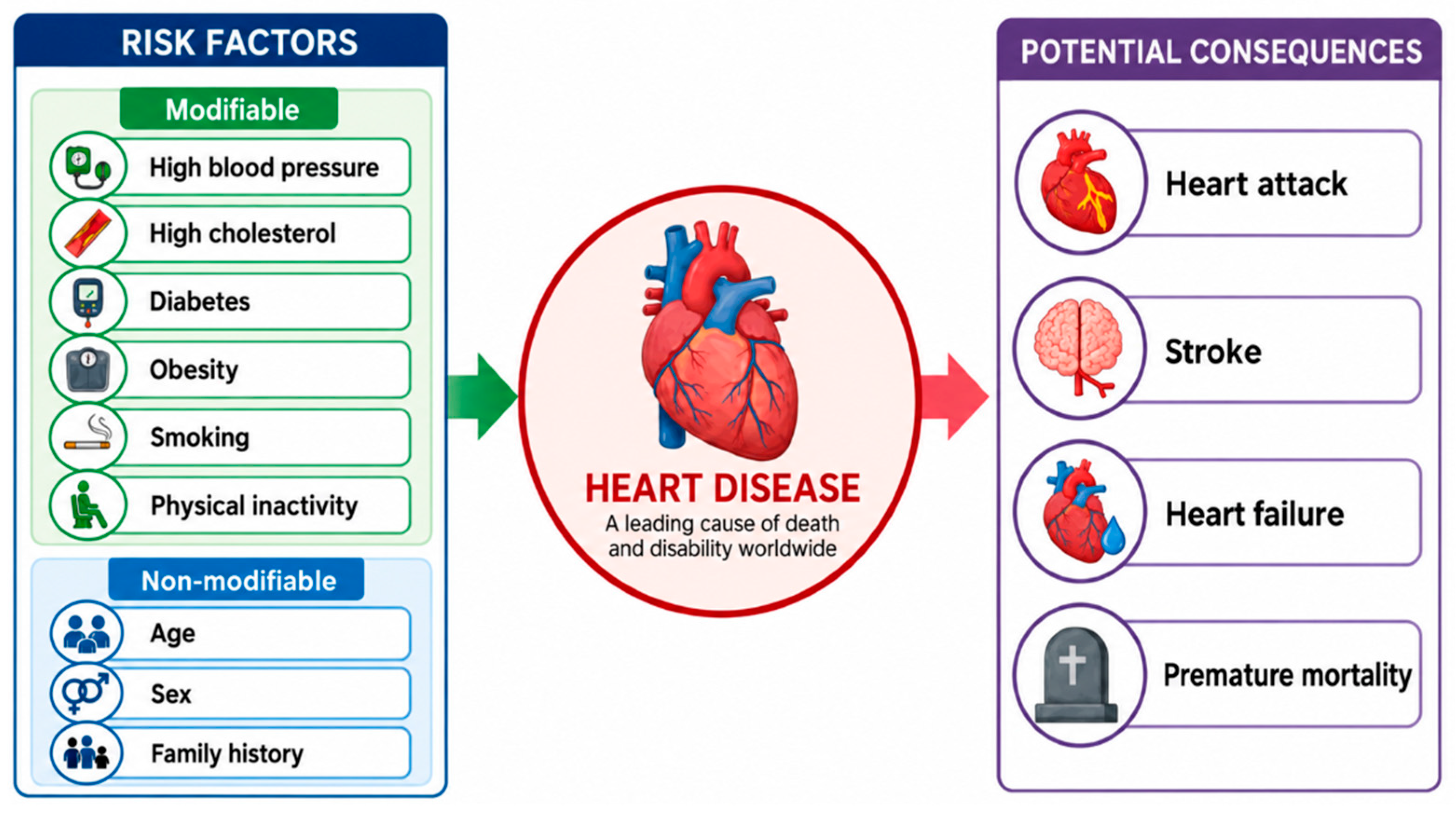
Figure 2.
Proposed Framework for Explainable GA-Optimized weighted soft-voting Heart Disease Prediction.
Figure 2.
Proposed Framework for Explainable GA-Optimized weighted soft-voting Heart Disease Prediction.
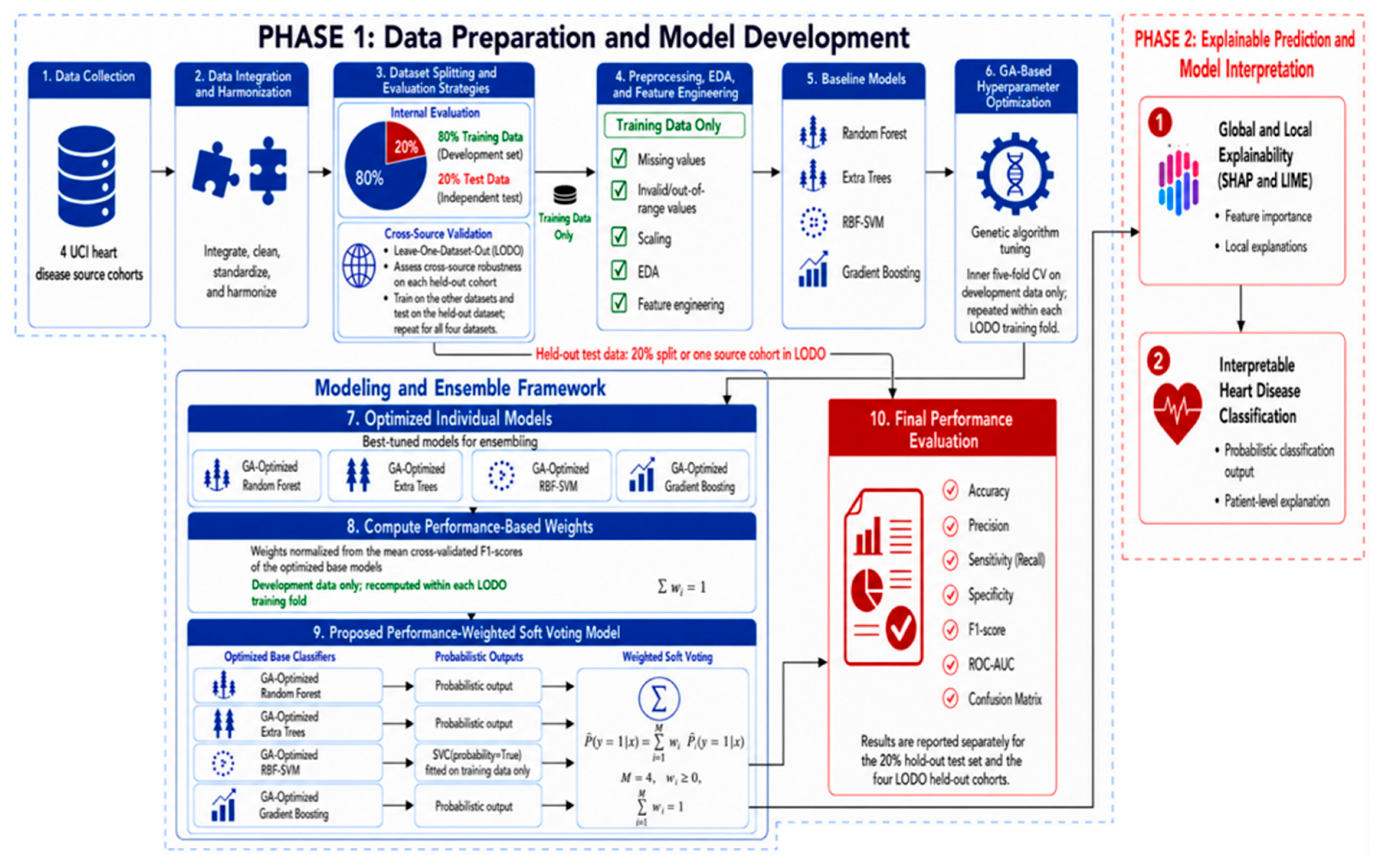
Figure 3.
Internal and Cross-Source Evaluation Strategies Employed in the Proposed Framework.
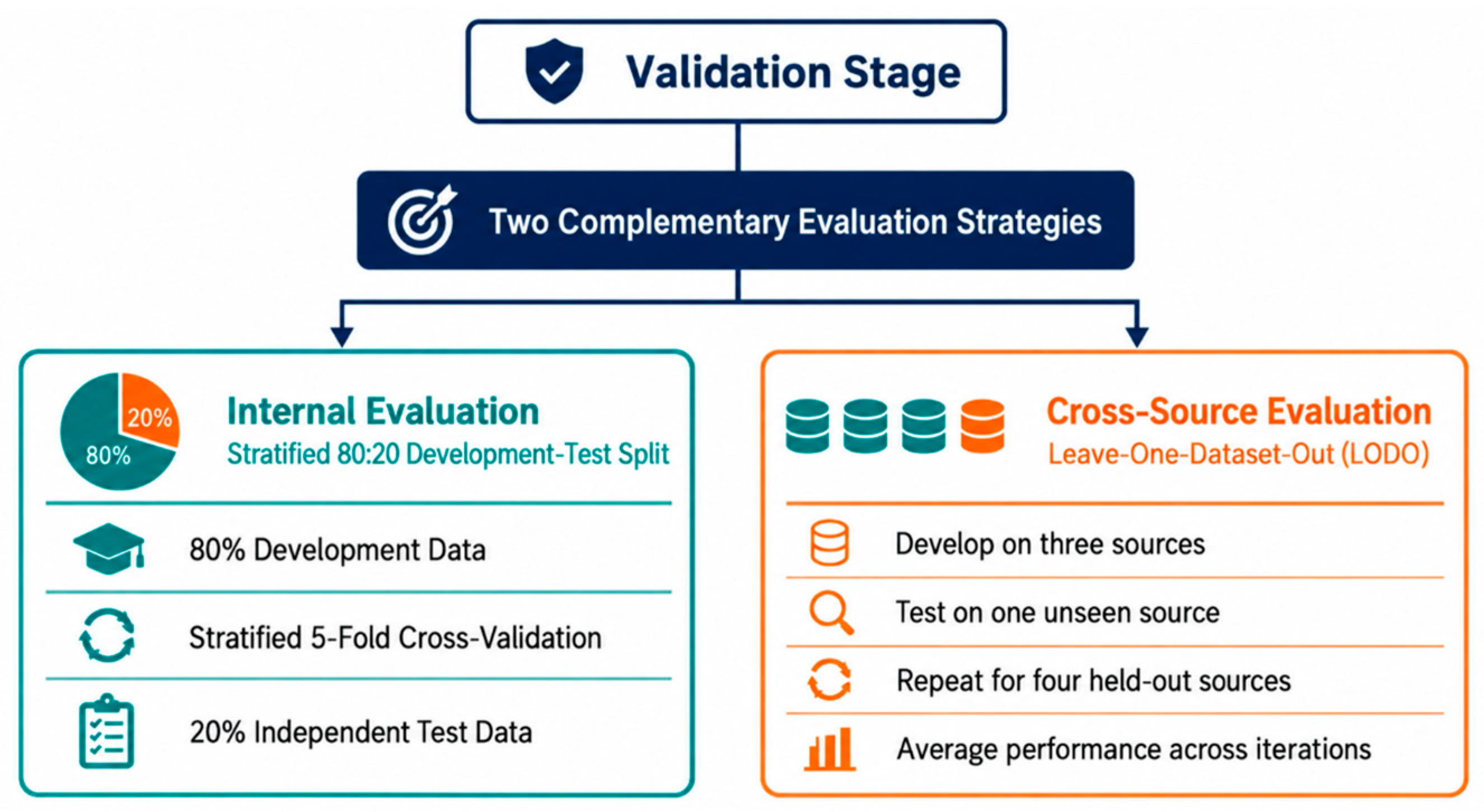
Figure 4.
Leakage-Controlled Data Preparation and Partitioning Workflow for the Four UCI Heart Disease Source Cohorts.
Figure 4.
Leakage-Controlled Data Preparation and Partitioning Workflow for the Four UCI Heart Disease Source Cohorts.
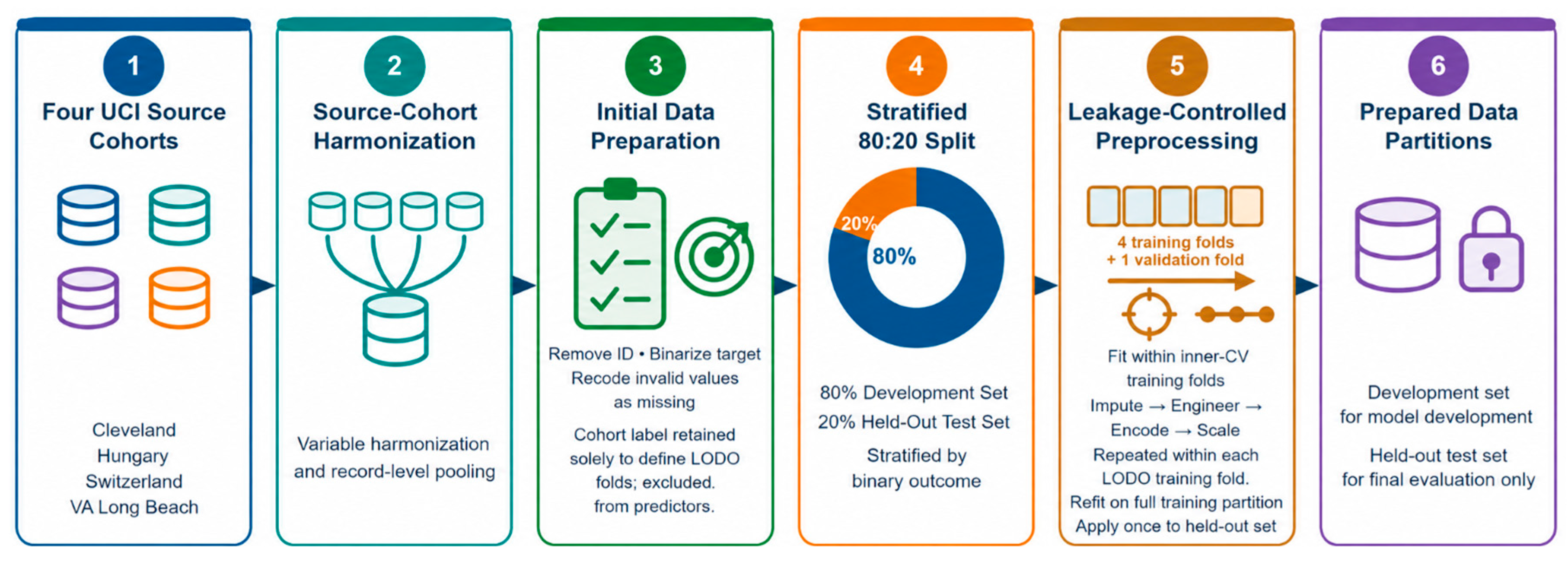
Figure 5.
Heart disease class and age-group distributions. (a) Overall class distribution. (b) Age-group distribution by class.
Figure 5.
Heart disease class and age-group distributions. (a) Overall class distribution. (b) Age-group distribution by class.
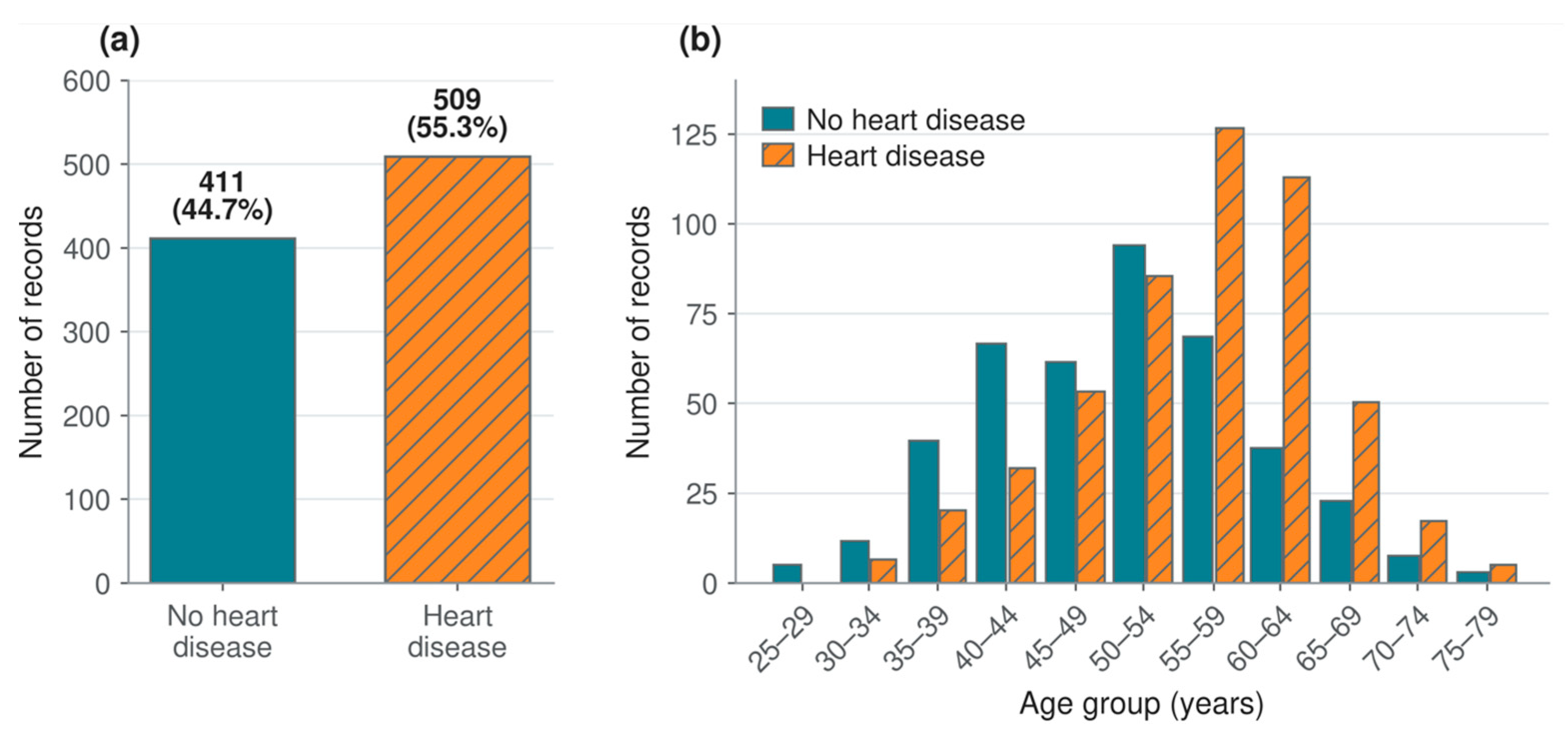
Figure 6.
Selected clinical-variable distributions by heart disease status: (a) resting blood pressure, (b) serum cholesterol, (c) maximum heart rate, and (d) oldpeak.
Figure 6.
Selected clinical-variable distributions by heart disease status: (a) resting blood pressure, (b) serum cholesterol, (c) maximum heart rate, and (d) oldpeak.
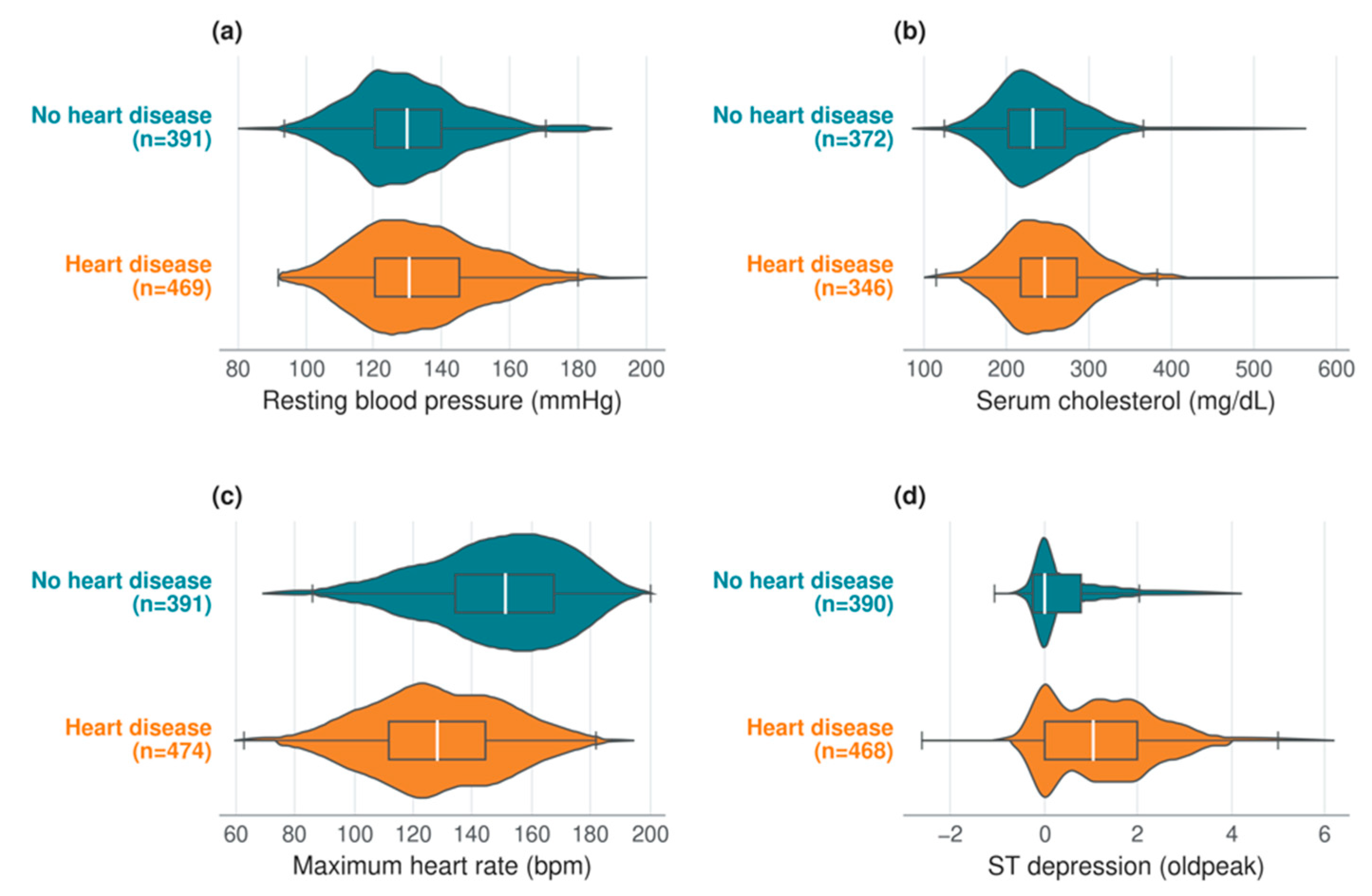
Figure 7.
Pearson correlation matrix of the selected numerical features and binary heart disease status.
Figure 7.
Pearson correlation matrix of the selected numerical features and binary heart disease status.
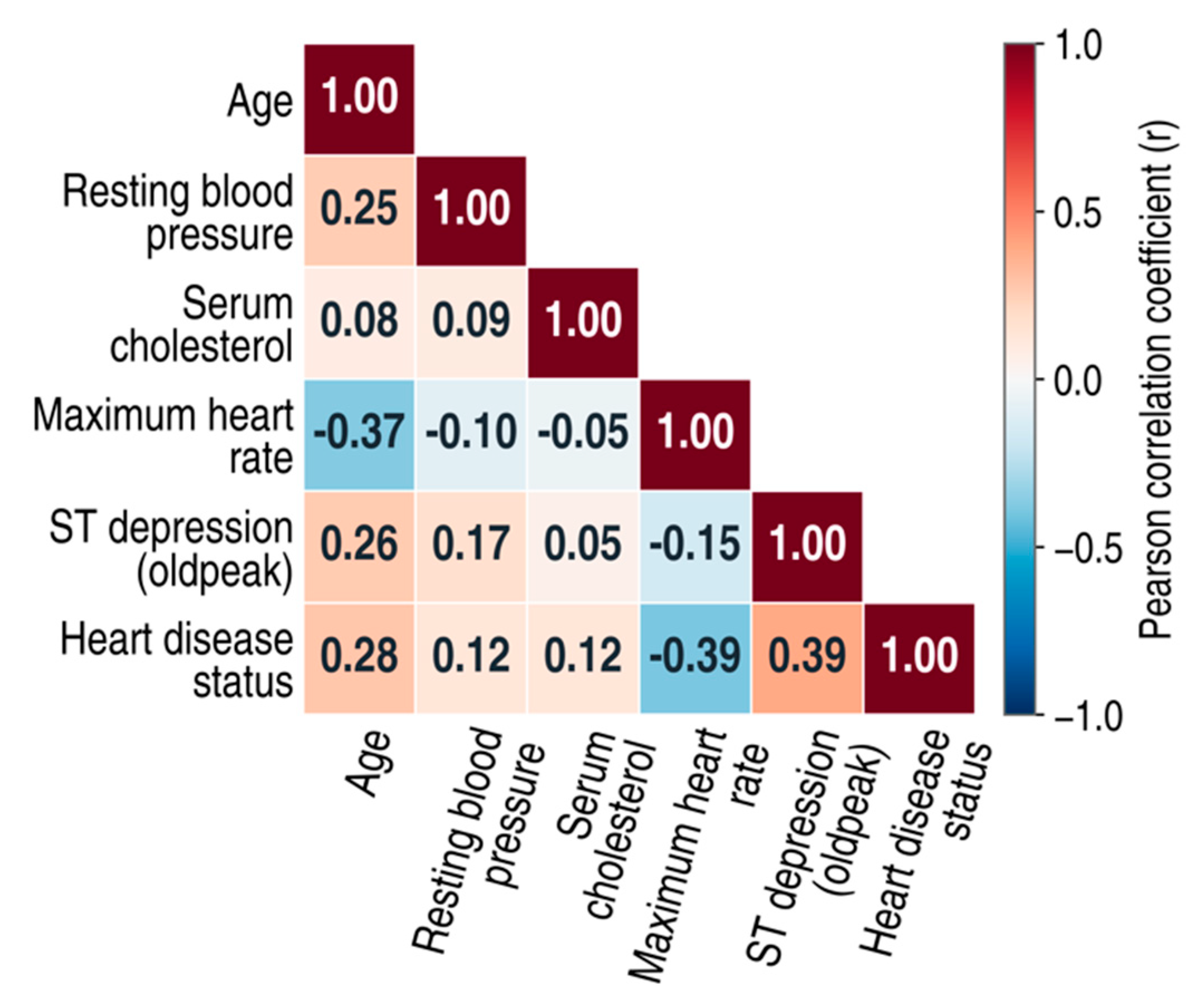
Figure 8.
Genetic algorithm-based hyperparameter optimization workflow using mean weighted F1-score under the 80:20 holdout and leave-one-source-cohort-out (LODO) validation schemes.
Figure 8.
Genetic algorithm-based hyperparameter optimization workflow using mean weighted F1-score under the 80:20 holdout and leave-one-source-cohort-out (LODO) validation schemes.
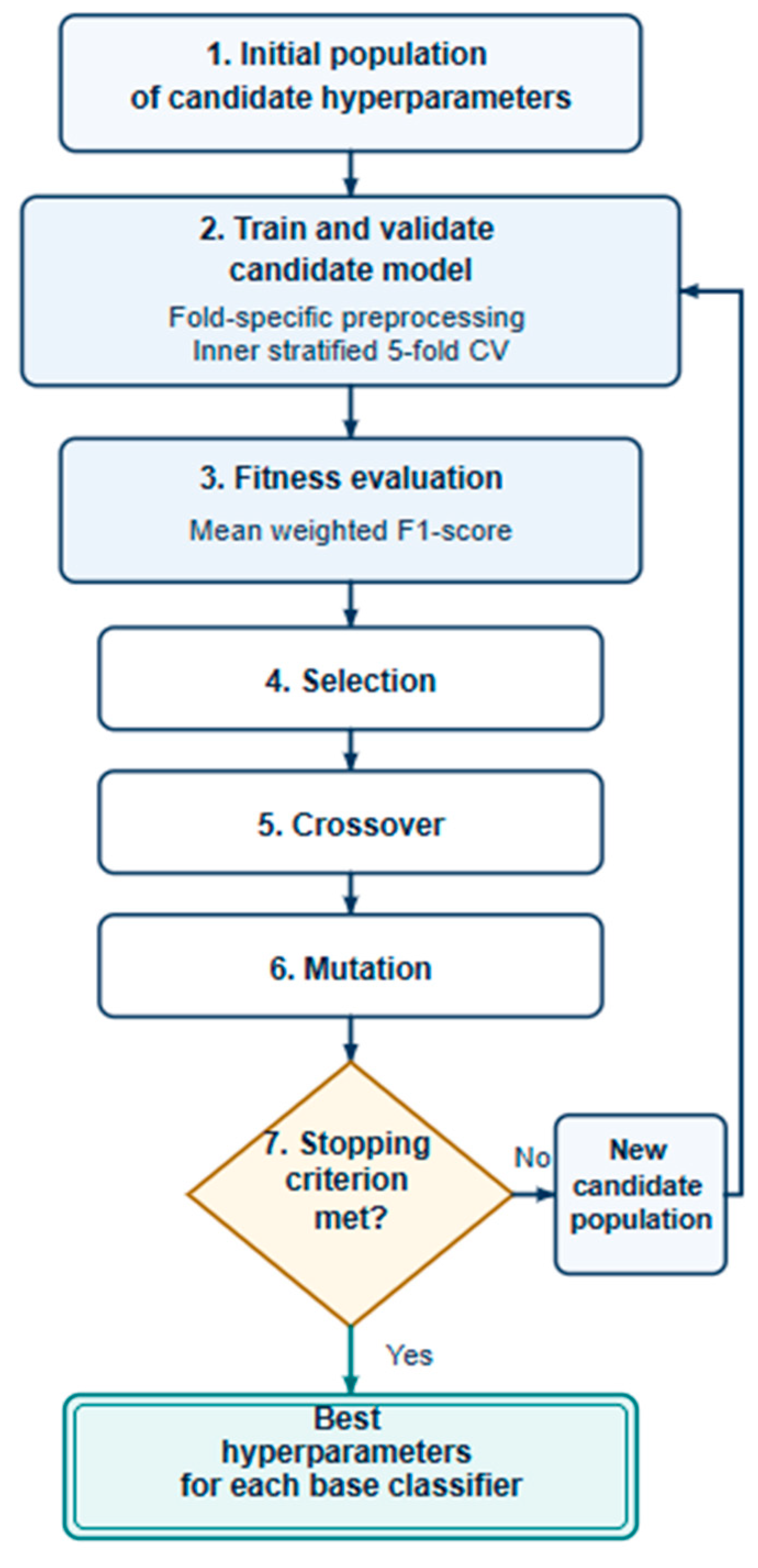
Figure 9.
Proposed performance-weighted soft-voting ensemble of GA-optimized base classifiers for heart disease prediction.
Figure 9.
Proposed performance-weighted soft-voting ensemble of GA-optimized base classifiers for heart disease prediction.
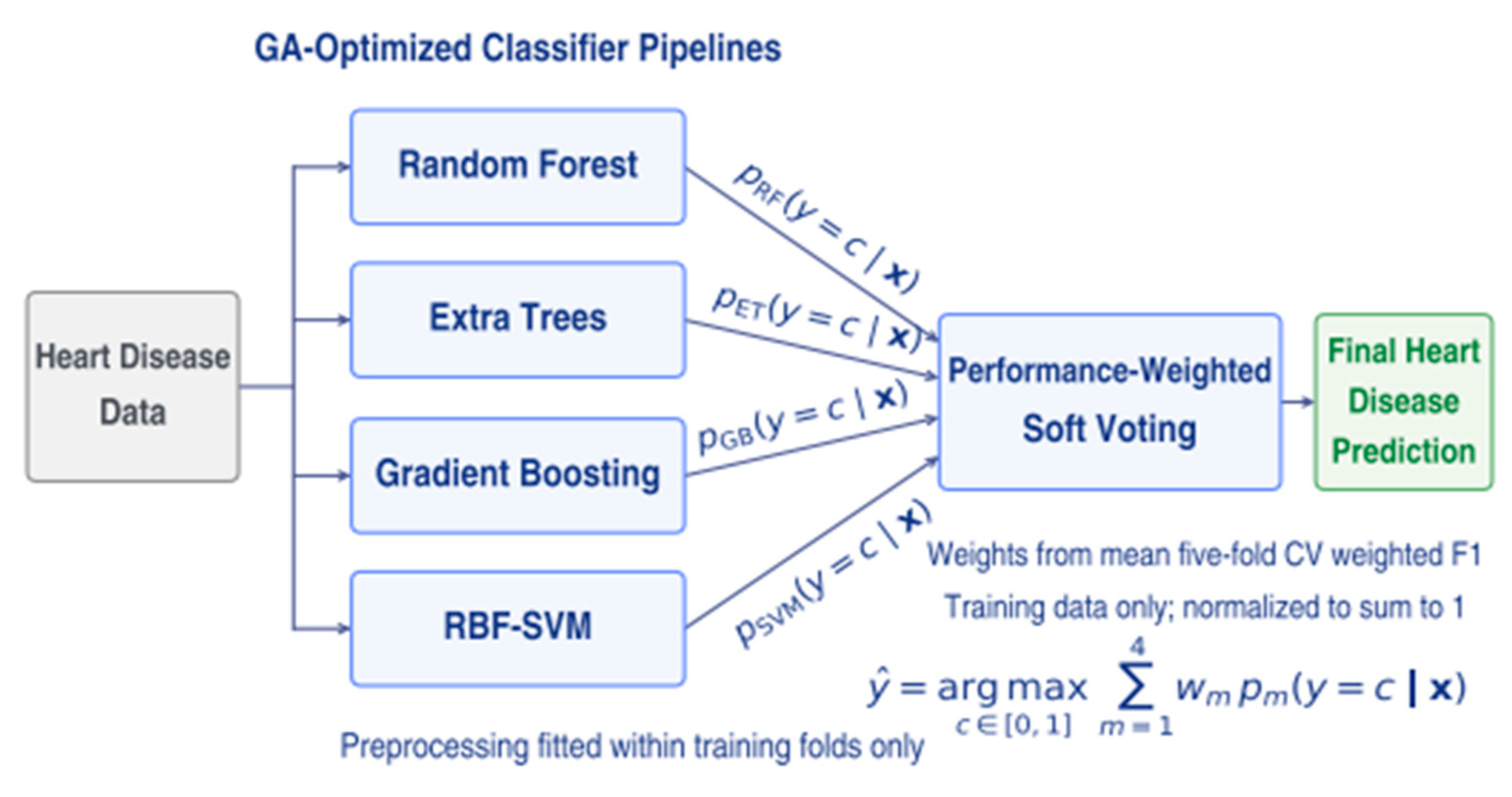
Figure 10.
Schematic illustration of the weighted-F1 improvement from the default to the GA-optimized configurations. Endpoints correspond to the cross-validated values reported in Table 10.
Figure 10.
Schematic illustration of the weighted-F1 improvement from the default to the GA-optimized configurations. Endpoints correspond to the cross-validated values reported in Table 10.
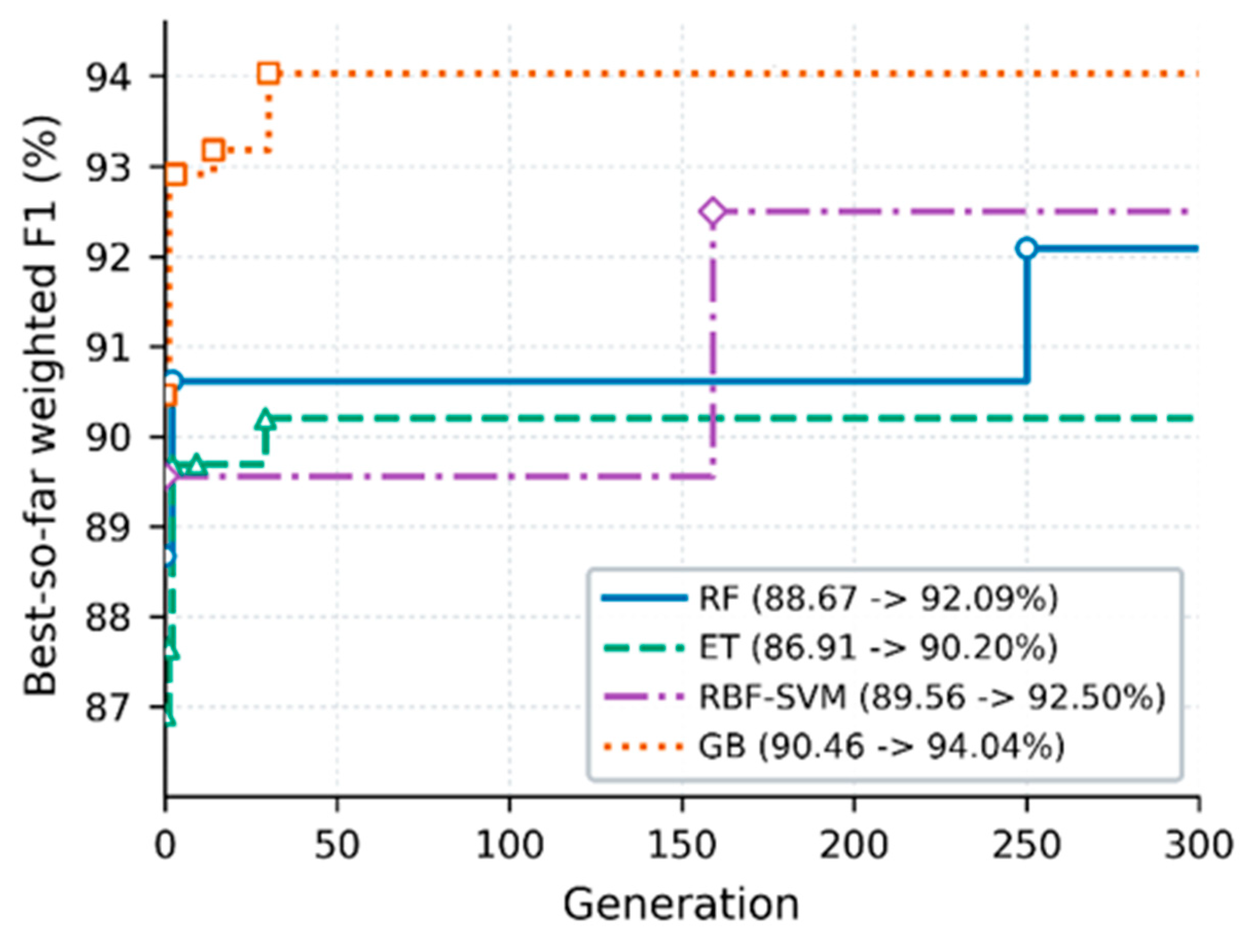
Figure 11.
Empirical receiver operating characteristic curves of the optimized base classifiers and the proposed PWSV ensemble on the held-out test set.
Figure 11.
Empirical receiver operating characteristic curves of the optimized base classifiers and the proposed PWSV ensemble on the held-out test set.
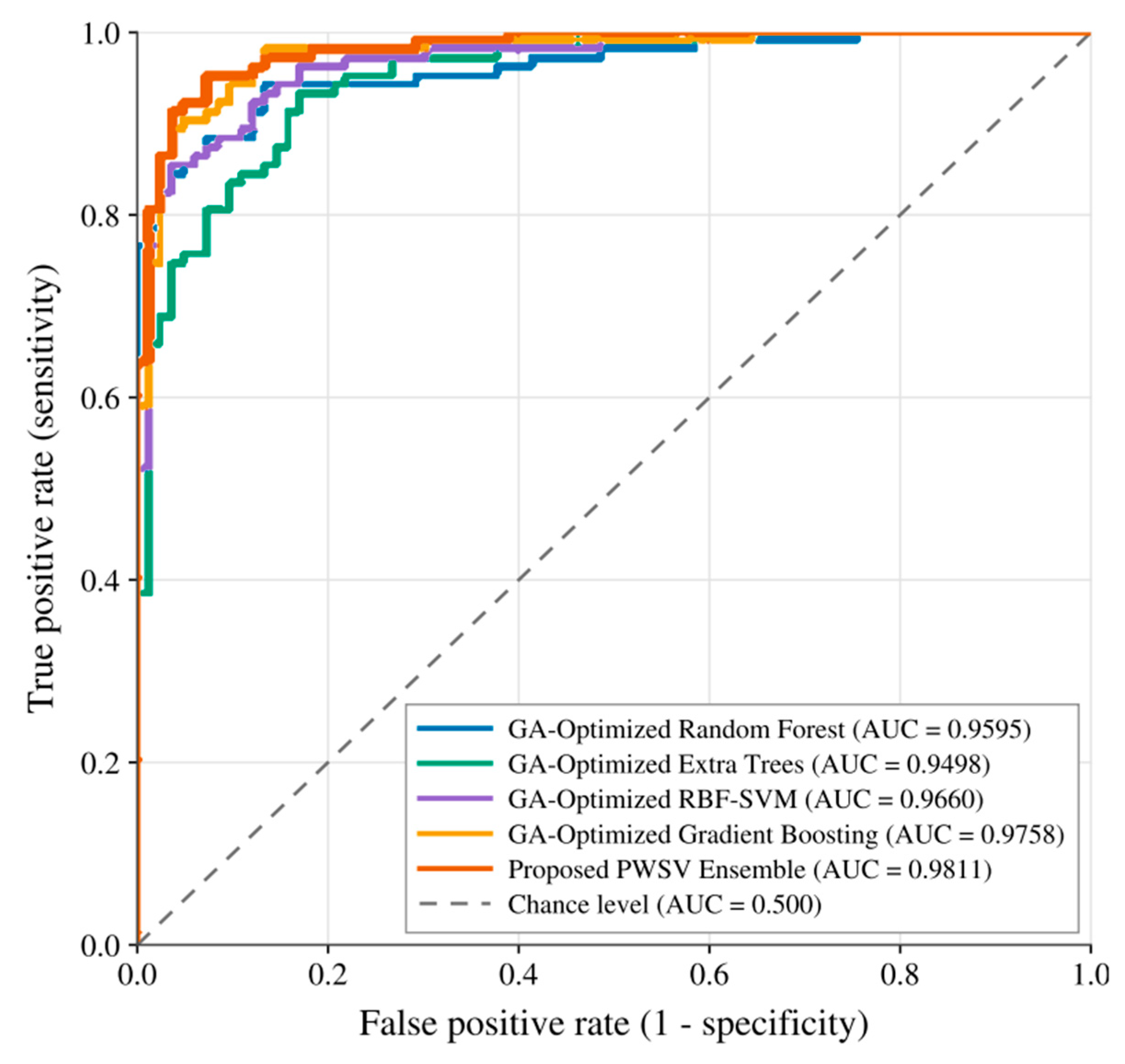
Figure 12.
Confusion matrices for (a) GA-RF, (b) GA-ET, (c) GA-RBF-SVM, (d) GA-GB, and (e) the proposed PWSV ensemble on the held-out test set at the predefined threshold of 0.50.
Figure 12.
Confusion matrices for (a) GA-RF, (b) GA-ET, (c) GA-RBF-SVM, (d) GA-GB, and (e) the proposed PWSV ensemble on the held-out test set at the predefined threshold of 0.50.
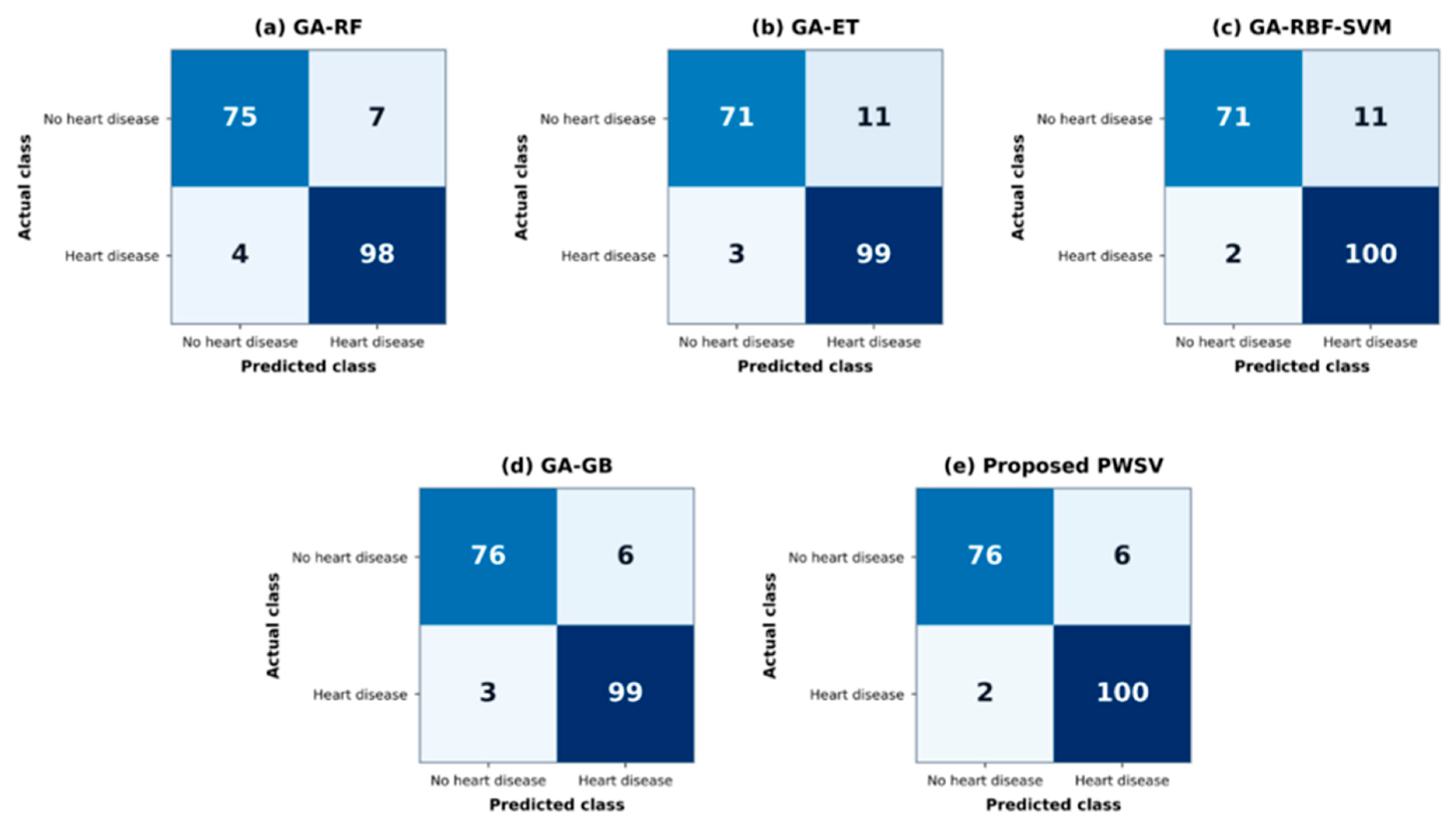
Figure 13.
Global probability-scale SHAP interpretation of the proposed PWSV ensemble on the stratified held-out test set. (a) Mean absolute SHAP values for the 15 most influential encoded predictors. (b) Beeswarm distribution of signed SHAP values, where positive and negative contributions respectively increase and decrease the predicted probability of heart disease. Colors represent encoded feature values from low (blue) to high (magenta). All attributions explain the final positive-class probability produced by the PWSV ensemble.
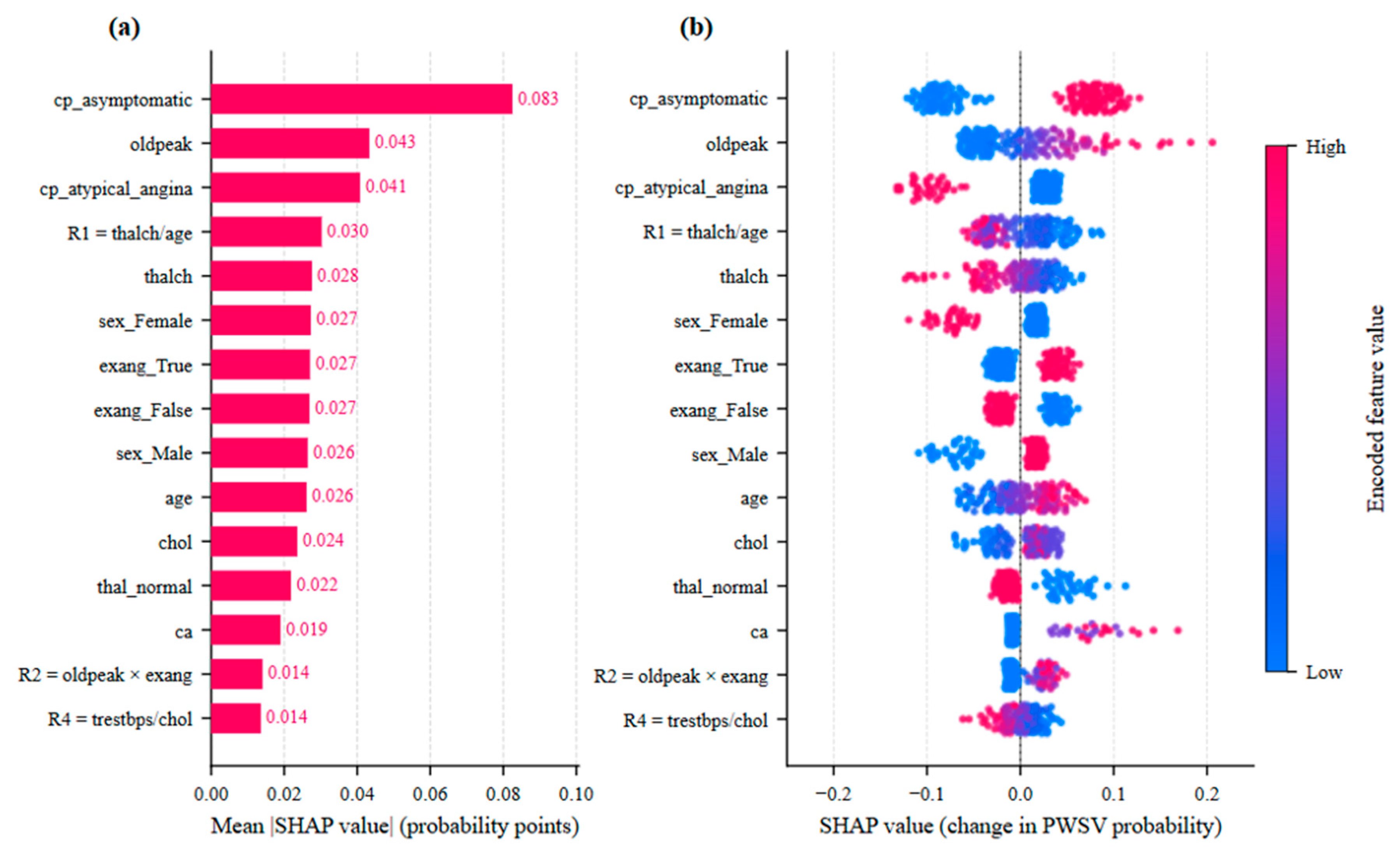
Figure 14.
Probability-scale SHAP explanations for the same two held-out test cases analyzed by LIME in Figure 15 below. (a) high-risk and (b) low-risk. Red and blue contributions respectively increase and decrease the PWSV probability.
Figure 14.
Probability-scale SHAP explanations for the same two held-out test cases analyzed by LIME in Figure 15 below. (a) high-risk and (b) low-risk. Red and blue contributions respectively increase and decrease the PWSV probability.
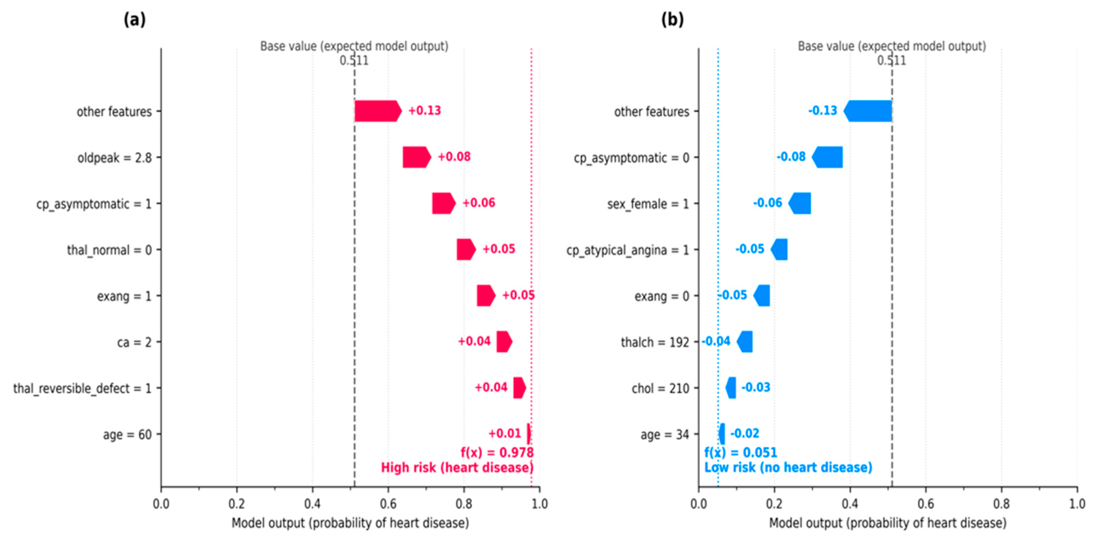
Figure 15.
LIME explanations for the same high- and low-risk test cases shown in Figure 14 above. Positive and negative contributions support and oppose the heart-disease class; the displayed probabilities are the original PWSV outputs.
Figure 15.
LIME explanations for the same high- and low-risk test cases shown in Figure 14 above. Positive and negative contributions support and oppose the heart-disease class; the displayed probabilities are the original PWSV outputs.
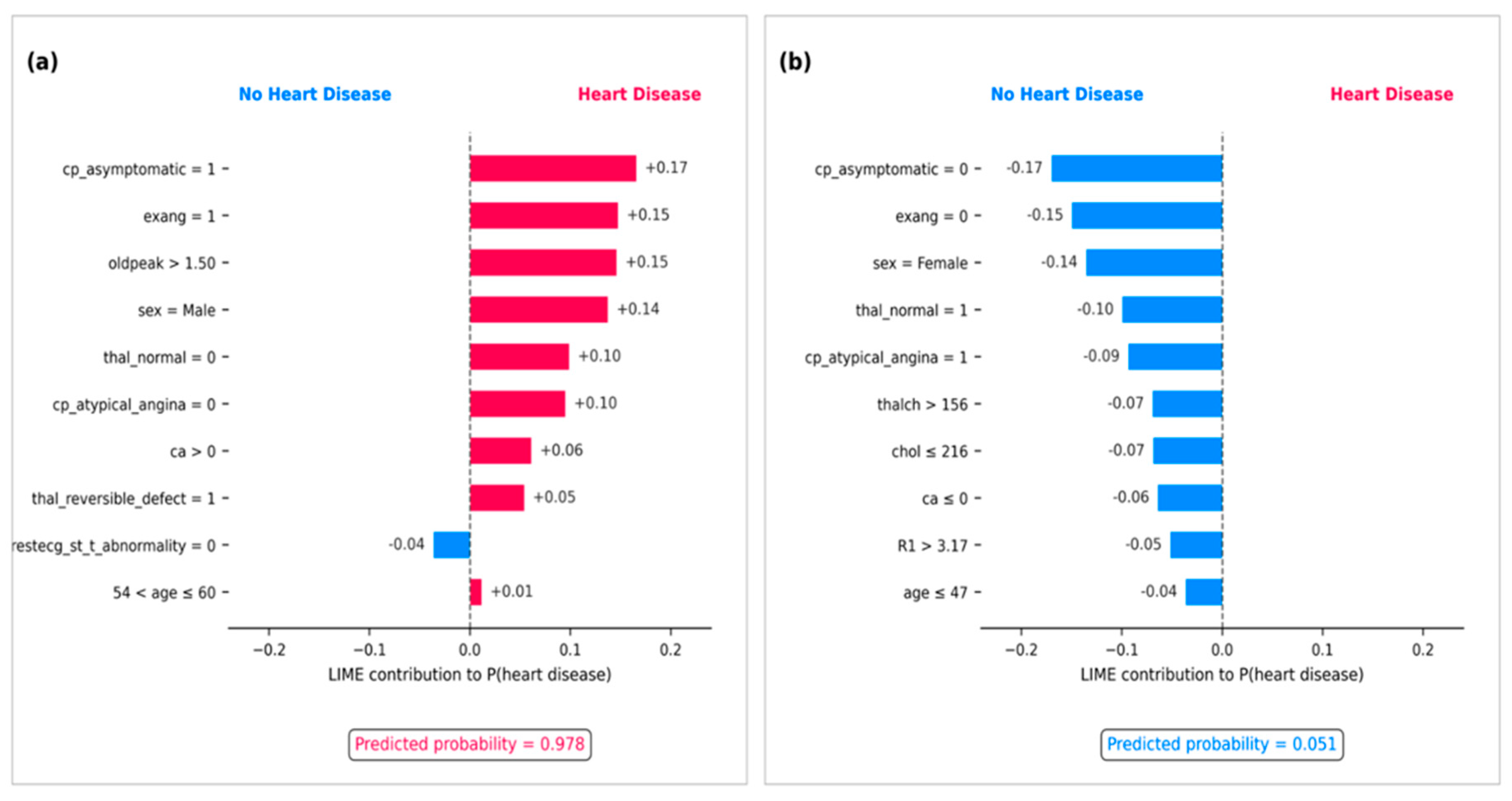
Figure 16.
Global SHAP–LIME concordance for the PWSV ensemble under nested LODO validation: (a) normalized importance of the ten leading predictors and (b) rank agreement across all 29 predictors (Spearman’s ρ = 0.867, p < 0.001). Importance was aggregated over 920 externally held-out observations, with the dataset identifier excluded from model inputs.
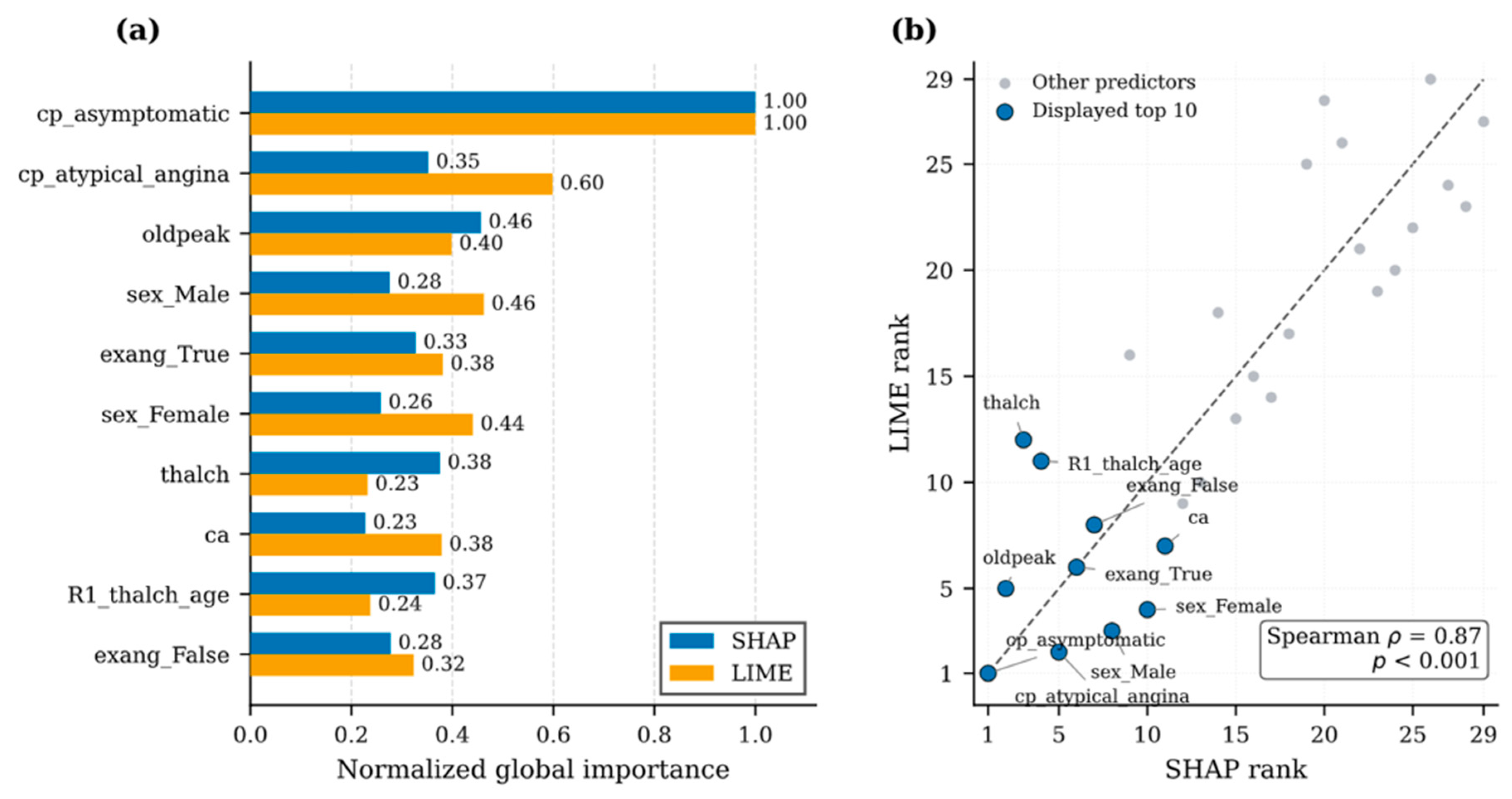

Table 1.
Comparative Summary of Previous Studies on Machine Learning-Based Heart Disease Prediction.
Table 1.
Comparative Summary of Previous Studies on Machine Learning-Based Heart Disease Prediction.
| Ref. | Dataset | Methodology | Best Result | Main Gap |
| [4] | BRFSS; Framingham; ZAS; clinical (n=700). | SMOTE, feature engineering, comparison of seven classifiers, tuned LightGBM, SHAP/LIME, and cross-dataset validation | BRFSS: Acc. 90.61%, AUROC 81.11%; clinical dataset: Acc. 91.0%, AUC 83.0%. | Performance varied across datasets; the 700-sample clinical evaluation used an internal random split rather than prospective multicenter validation. |
| [5] | Cleveland; Statlog. | Preprocessing/FE; LR/DT/KNN/RF/AdaBoost/SVM; grid/random search; 10-fold CV. | SVM: Acc. 92% (Cleveland), 91.18% (Statlog). | No combined ensemble or XAI; only 2 small benchmarks. |
| [10] | Kaggle heart dataset | Bayesian hyperparameter optimization, XGBoost-LightGBM voting ensemble, SHAP, and LIME | Voting ensemble: test Acc. 96.22%, AUC 95.75%. | Evaluated on a single pooled Kaggle dataset without source-wise or independent external validation. |
| [11] | Cleveland; IEEE DataPort. | Six classifiers, GridSearchCV, five-fold CV, and soft voting | Soft voting: Acc. 93.44% (Cleveland), 95.00% (IEEE DataPort). | No XAI analysis or source-wise external validation. |
| [12] | UCI Cleveland dataset | NB, DT, KNN, and RF evaluated using the 14 commonly selected Cleveland attributes. | KNN achieved approximately 90.79% accuracy | Only selected attributes and a limited set of classifiers were examined; no ensemble, optimization, or XAI. |
| [16] | UCI heart disease dataset |
ML and deep-learning models with normalization and Isolation Forest | Deep learning achieved 94.2% accuracy | Pooled UCI benchmark (4 sources); no source-wise validation, ensemble voting, or XAI. |
| [17] | Bangladesh clinical data (n=59). | Correlation-based feature selection, seven classifiers, and 10-fold cross-validation | RF with selected features achieved 90% accuracy | Small dataset (n=59); no tuning, ensemble, XAI, or independent validation. |
| [19] | UCI Cleveland heart disease dataset. | SVM, GB, XGBoost, MLP, LightGBM, SHAP, and LIME | XGBoost achieved 92% accuracy and 0.93 AUC | Single small dataset; no external validation or combined ensemble. |
| [20] | Cleveland dataset | Probability-based regression layers combined with SVM and ANN | Regression layers + SVM: Acc. 95.55%. | Evaluated only on the small Cleveland dataset, without independent external validation or XAI analysis. |
| [23] | Three combined Kaggle datasets | RF, Extra Trees, XGBoost, CatBoost, and Grid/Random Search CV | Extra Trees achieved 98.15% accuracy | 3 pooled Kaggle datasets; random holdout; no source-wise external validation or XAI. |
| [24] | KAMIR-NIH dataset | RF, ET, GBM, hyperparameter tuning, and soft voting | 90.93% accuracy and 99.61% AUC | The clinical dataset is not publicly available, and the study focused on MACE prediction rather than general heart-disease classification. |
| [25] | Combined IEEE DataPort dataset | 10 classifiers screened; RF/ET/GB/XGBoost stacking; 80:20 split; 10-fold CV. | Stacked ensemble achieved 92.34% accuracy | 5 pooled datasets; CV used; no source-wise/external validation or SHAP/LIME. |
| [27] | Cleveland; private clinical data. | 10 classifiers; 3 feature selectors; SMOTE; tuning; XGBoost; SHAP. | 97.57% accuracy and 98% AUC | Pooled public/private data; no fully independent external validation; best: single XGBoost, not voting. |
Table 2.
Clinical Variables in the UCI disease dataset.
| Variable | Type | Values / Range | Clinical Description |
| Age | Continuous | 28 – 77 years | Age of the patient |
| Sex | Categorical | M: Male | Biological sex of the patient |
| F: Female | |||
| ChestPainType (cp) | Categorical | TA: Typical Angina | Type of chest pain experienced by the patient |
| ATA: Atypical Angina | |||
| NAP: Non-Anginal Pain | |||
| ASY: Asymptomatic | |||
| RestingBP (trestbps) | Continuous | 80 to 200 mm Hg | Resting blood pressure |
| Cholesterol (chol) | Continuous | 85 to 603 mg/dL | Serum cholesterol level |
| FastingBS (fbs) | Binary | 1: >120 mg/dL | Fasting blood sugar indicator |
| 0: ≤120 mg/dL | |||
| RestingECG (restecg) | Categorical | Normal | Resting electrocardiographic results |
| ST: ST-T wave abnormality | |||
| LVH: Left ventricular hypertrophy | |||
| MaxHR (thalch) | Continuous | 60–202 | Maximum heart rate achieved |
| ExerciseAngina (exang) | Binary | Y: Yes | Exercise-induced angina |
| N: No | |||
| Oldpeak | Continuous | -2.6 to 6.2 | ST depression induced by exercise |
| ST_Slope | Categorical | Up: Upsloping | Slope of the peak exercise ST segment |
| Flat: Flat | |||
| Down: Down sloping | |||
| ca | Ordinal | 0 – 3 | Number of major vessels colored by fluoroscopy |
| thal | Categorical | Normal | Thallium-201 stress scintigraphy result |
| Fixed defect | |||
| Reversible defect | |||
| HeartDisease (num) | Target (raw ordinal; modeled binary) | Raw: 0–4; Modeled: 0/1 | Raw 0 indicates disease absence, whereas raw values 1–4 indicate disease presence; recoded as 0 = absence and 1 = presence. |
Table 3.
Leave-One-Dataset-Out Cross-Source Evaluation Configuration.
| Fold | Training Source | Testing Source |
| 1 | Hungary + Switzerland + VA Long Beach | Cleveland |
| 2 | Cleveland + Switzerland + VA Long Beach | Hungary |
| 3 | Cleveland + Hungary + VA Long Beach | Switzerland |
| 4 | Cleveland + Hungary + Switzerland | VA Long Beach |
Table 4.
Missing Values After Invalid-Zero Recoding and Before Imputation (N = 920).
| Feature | Original missing | Invalid zeros | Missing after recoding, n | Missing after recoding, % |
| ca | 611 | 0 | 611 | 66.41% |
| thal | 486 | 0 | 486 | 52.83% |
| slope | 309 | 0 | 309 | 33.59% |
| chol | 30 | 172 | 202 | 21.96% |
| fbs | 90 | 0 | 90 | 9.78% |
| Oldpeak | 62 | 0 | 62 | 6.74% |
| trestbps | 59 | 1 | 60 | 6.52% |
| exang | 55 | 0 | 55 | 5.98% |
| thalch | 55 | 0 | 55 | 5.98% |
| resecg | 2 | 0 | 2 | 0.22% |
Table 5.
Baseline Models and Their Configurations.
| Model | Its characteristics |
| RF | Bagging-Based ensemble for stable prediction |
| ET | Randomized tree ensemble to reduce variance |
| Gradient Boosting | Sequential boosting model for error correction |
| RBF-SVM | Nonlinear classifier for complex decision boundaries |
Table 6.
Feature Representations evaluated.
| Feature Representation | Encoded columns | Included Predictors |
| Original Feature (13) | 25 | (age, sex, cp, trestbps, chol, fbs, restecg, thalch, exang, oldpeak, slope, ca, thal) |
| Original + Source (14) | 29 | 13 Original Feature + (dataset_source) |
| Original + Engineered (17) | 29 | 13 Original Feature + (R1, R2, R3, R4) |
| Encoded Full Feature Space (18)1 | 33 | 13 Original Feature + (R1, R2, R3, R4) + (dataset_source) |
1The same categorical-encoding procedure was applied to all feature representations. The dimensionality of 33 refers to the full representation after preprocessing and encoding.
Table 7.
Stratified five-fold cross-validation performance of the baseline classifiers across the evaluated feature representations on the development set.
Table 7.
Stratified five-fold cross-validation performance of the baseline classifiers across the evaluated feature representations on the development set.
| Model | Feature Set | Accuracy (%) * | Precision (%) * | Recall (%) * | Positive-Class F1 (%) * | ROC-AUC (%) * |
| Random Forest | Original Feature | 82.61±2.43 | 83.02±5.40 | 86.27±3.5 | 84.62±1.26 | 91.37±3.12 |
| Original + Source | 81.52±2.71 | 81.48±5.08 | 86.27±3.01 | 83.81±1.70 | 90.32±2.91 | |
| Original + Engineered | 84.78±1.82 | 84.26±4.79 | 89.22±5.19 | 86.67±1.37 | 91.97±2.91 | |
| Encoded Full Feature Space | 83.15±1.75 | 83.81±4.25 | 86.27±5.85 | 85.02±1.72 | 91.48±3.53 | |
| Extra Trees | Original Feature | 81.52±4.20 | 81.48±5.94 | 86.27±4.40 | 83.81±3.18 | 90.54±3.65 |
| Original + Source | 82.07±3.69 | 81.65±6.25 | 87.25±4.96 | 84.36±2.75 | 90.57±3.14 | |
| Original + Engineered | 82.61±3.55 | 81.82±5.33 | 88.24±5.65 | 84.91±3.11 | 89.40±2.58 | |
| Encoded Full Feature Space | 82.07±2.80 | 83.50±5.16 | 84.31±6.12 | 83.90±2.47 | 90.91±3.88 | |
| RBF-SVM | Original Feature | 81.52±1.48 | 80.36±3.91 | 88.24±4.15 | 84.11±0.77 | 89.75±2.37 |
| Original + Source | 82.61±2.23 | 80.70±3.99 | 90.20±3.81 | 85.19±1.75 | 89.22±2.67 | |
| Original + Engineered | 85.33±2.67 | 82.61±4.88 | 93.14±3.82 | 87.56±1.85 | 92.06±2.53 | |
| Encoded Full Feature Space | 84.24±1.23 | 82.88±4.03 | 90.20±5.97 | 86.38±1.28 | 91.51±2.43 | |
| Gradient Boosting | Original Feature | 83.15±1.85 | 82.57±4.35 | 88.24±4.11 | 85.31±0.88 | 91.03±2.29 |
| Original + Source | 82.07±2.09 | 80.53±3.99 | 89.22±3.49 | 84.65±1.36 | 90.57±1.49 | |
| Original + Engineered | 86.96±1.42 | 86.79±3.65 | 90.20±4.11 | 88.46±0.88 | 92.36±1.51 | |
| Encoded Full Feature Space | 84.24±1.54 | 84.76±3.84 | 87.25±5.82 | 85.99±1.53 | 91.80±2.15 |
* Please note that all the figures are expressed as mean ± SD (%). Precision, recall, and F1 score refer to the positive heart-disease class. All the preprocessing procedures were done on the training dataset in each fold, and the independent test dataset was not included when selecting the feature representation. Boldface denotes the highest mean for each metric within each classifier block and does not imply statistical significance.
Table 8.
Baseline hyperparameter configurations.
| Model | Baseline Hyperparameter |
| RF | max_depth = None, max_features = sqrt, min_samples_split = 2, min_samples_leaf = 1, n_estimators = 100, criterion = gini |
| ET | max_depth = 10, max_features = sqrt, min_samples_split = 5, min_samples_leaf = 1, n_estimators = 100, criterion = gini |
| RBF-SVM | C = 1, gamma = 0.1, kernel = rbf |
| GB | n_estimators = 100, learning_rate = 0.05, max_depth = 3, subsample = 1.0, min_samples_split = 2, and min_samples_leaf = 1. |
Table 9.
GA-optimized configurations and cv weighted F1-score.
| Model | GA-Optimized Hyperparameters | CV Weighted F1-Score (%) 1 |
| RF | max_depth = 9, max_features = sqrt, min_samples_split = 4, min_samples_leaf = 2, n_estimators = 300, criterion = entropy | 92.09±2.09 |
| ET | max_depth = 18, max_features = sqrt, min_samples_split = 3, min_samples_leaf = 1, n_estimators = 400, criterion = gini | 90.20±3.50 |
| RBF-SVM | C = 10, gamma = 0.01, kernel = rbf, probability = true | 92.50±1.62 |
| GB | n_estimators = 150, learning_rate = 0.03, max_depth = 3, subsample = 0.9, min_samples_split = 4, min_samples_leaf = 3. | 94.04±2.95 |
1Fitness values are reported as mean ± standard deviation (%) across the five stratified validation folds.
Table 10.
Cross-validated performance comparison of the baseline and GA-optimized models.
| Model | Configuration | Accuracy% | Precision% | Recall% | Weighted F1 (%) | ROC-AUC% | ∆F1 |
| RF | Baseline (default) | 86.78±1.82 | 87.26±4.79 | 89.22±5.19 | 88.67±1.95 | 92.97±2.93 | +3.42 |
| GA-Optimized | 91.30±3.54 | 89.34±5.32 | 95.02±2.44 | 92.09±2.09 | 94.65±2.43 | ||
| ET | Baseline (default) | 84.61±3.20 | 83.82±5.67 | 90.24±4.46 | 86.91±3.41 | 91.40±2.79 | +3.29 |
| GA-Optimized | 89.67±3.22 | 86.34±5.31 | 94.41±3.36 | 90.20±3.50 | 93.18±2.49 | ||
| RBF-SVM | Baseline (default) | 87.33±2.97 | 84.61±4.65 | 95.14±2.43 | 89.56±2.12 | 94.06±2.85 | +2.94 |
| GA-Optimized | 92.39±1.63 | 87.41±3.14 | 95.22±4.29 | 92.50±1.62 | 95.74±2.02 | ||
| GB | Baseline (default) | 88.96±2.09 | 88.79±4.43 | 92.20±3.73 | 90.46±2.27 | 94.36±1.92 | +3.58 |
| GA-Optimized | 94.02±2.76 | 92.02±5.58 | 94.14±3.02 | 94.04±2.95 | 96.88±1.92 |
Table 11.
Cross-validated weighted F1-score and normalized ensemble weights.
| Model | Optimized CV weighted F1-score (%) | Assigned Weight |
| RF | 92.09±2.09 | 0.24968 |
| ET | 90.20±3.50 | 0.24456 |
| RBF-SVM | 92.50±1.62 | 0.25079 |
| GB | 94.04±2.95 | 0.25497 |
| Total | --- | 1.00000 |
Table 12.
Performance Comparison of Optimized models and proposed Soft Voting Ensemble.
| Model | Accuracy | Precision | Recall | F1-Score | ROC-AUC |
| GA-optimized RF | 94.02% | 93.33% | 96.08% | 94.69% | 95.95% |
| GA-optimized ET | 92.39% | 90.00% | 97.06% | 93.40% | 94.98% |
| GA-optimized RBF-SVM | 92.93% | 90.09% | 98.04% | 93.90% | 96.60% |
| GA-optimized GB | 95.11% | 94.29% | 97.06% | 95.65% | 97.58% |
| Proposed performance- Weighted Soft Voting (PWSV) | 95.65% | 94.34% | 98.04% | 96.15% | 98.11% |
Table 13.
Composition of the Leave-One-Dataset-Out validation iterations.
| Held-out test dataset | Training datasets | Training case | Test cases | Heart disease cases, n (%) |
| Cleveland | Hungary + Switzerland + VA Long Beach | 616 | 304 | 139 (45.72%) |
| Hungary | Cleveland + Switzerland + VA Long Beach | 627 | 293 | 106 (36.18%) |
| Switzerland | Cleveland + Hungary + VA Long Beach | 797 | 123 | 115 (93.50%) |
| VA Long Beach | Cleveland + Hungary + Switzerland | 720 | 200 | 149 (74.50%) |
Table 14.
Performance of the Proposed PWSV Framework Under Lodo Evaluation.
| Held-out test dataset | Accuracy | Precision | Recall | F1-score | AUC |
| Cleveland | 93.75% | 91.16% | 92.91% | 92.03% | 95.62% |
| Hungary | 92.15% | 90.65% | 91.33% | 91.00% | 94.50% |
| Switzerland | 88.62% | 85.84% | 87.32% | 86.57% | 89.92% |
| VA Long Beach | 89.00% | 84.57% | 87.19% | 85.86% | 90.02% |
Table 15.
Contextual Comparison with Related Heart-Disease Prediction Studies.
| Ref. | Dataset | Classifiers Used | Methodology Used | Reported Accuracy | F1-score | AUC |
| [5] | Cleveland, n=303; validated on Statlog, n=270 | DT, RF, SVM, LR, AdaBoost, and KNN | 75:25 holdout, hyperparameter tuning, external Statlog validation, and 10-fold CV | 92.00% Cleveland; 91.18% Statlog | 92.00% Cleveland; 92.69% Statlog | 91.00% Cleveland; 90.36% Statlog |
| [11] | Cleveland and IEEE Dataport comprehensive datasets | RF, KNN, LR, NB, GB, AdaBoost, and SVE | GridSearchCV with 5-fold CV and Soft Voting | 93.44% Cleveland; 95.00% IEEE | NR* | NR* |
| [19] | UCI Cleveland, n=303, 14 attributes | SVM, GB, XGBoost, MLP, and LightGBM | ML classification with SHAP and LIME; validation protocol NR | 92.00% | 90.50% | 93.00% |
| [24] | KAMIR-NIH ACS registry; 2-year MACE, n=11,189 | RF, ET, GBM, weighted SVE | 70:30 holdout + 5-fold stratified CV | 90.93% | 90.95% | 99.61% |
| [25] | IEEE Dataport comprehensive dataset, n=1,190 | RF, ET, XGBoost, and GBM stacked ensemble | 80:20 holdout; 10-fold CV for base-model selection | 92.34% | 92.74% | 92.28% |
| [27] | Cleveland plus private clinical dataset, n=503 | NB, SVM, Voting, XGBoost, AdaBoost, Bagging, DT, KNN, RF, and LR | Feature selection, SMOTE, hyperparameter tuning, 75:25 holdout, and SHAP | 97.57% | 92.68% | 98.00% |
| Proposed | Integrated UCI heart disease dataset: Cleveland, Hungarian, Switzerland, and VA Long Beach | GA-optimized performance-weighted Soft Voting: RF, ET, RBF-SVM, and GB | Stratified 80:20 held-out evaluation; inner five-fold CV for GA optimization and ensemble-weight estimation; four-source LODO evaluation; SHAP and LIME explanations. | 95.65% | 96.15% | 98.11% |
*Note: NR denotes not reported. All values were reproduced as reported in the original studies and were not recomputed. Because the studies differ in prediction targets, dataset composition, preprocessing procedures, and validation protocols, the comparison is contextual and should not be interpreted as a direct head-to-head ranking.
Disclaimer/Publisher’s Note: The statements, opinions and data contained in all publications are solely those of the individual author(s) and contributor(s) and not of MDPI and/or the editor(s). MDPI and/or the editor(s) disclaim responsibility for any injury to people or property resulting from any ideas, methods, instructions or products referred to in the content. |
© 2026 by the authors. Licensee MDPI, Basel, Switzerland. This article is an open access article distributed under the terms and conditions of the Creative Commons Attribution (CC BY) license (http://creativecommons.org/licenses/by/4.0/).
Copyright: This open access article is published under a Creative Commons CC BY 4.0 license, which permit the free download, distribution, and reuse, provided that the author and preprint are cited in any reuse.