
Submitted:
13 October 2026
Posted:
14 October 2026
You are already at the latest version
Abstract
Spatiotemporal models of chimeric antigen receptor T-cell therapy can clarify how interacting biological mechanisms shape therapeutic response, but global sensitivity analysis and response-regime mapping require many computationally expensive simulations. We developed an adaptive surrogate-assisted algorithm that combines these tasks within a single computational framework. Independent Gaussian process surrogates were constructed for the final and minimum normalised tumour burdens, and new simulations were selected according to surrogate uncertainty and proximity to regime boundaries. Surrogates trained on 120 simulations achieved normalised root-mean-square errors of 0.00148 and 0.01058 on a fully held-out test set. Regime classification agreed with direct simulations at all 30 test points and 12 additional points near regime boundaries. The stopping criterion was first satisfied after 84 training simulations, while the advantage of adaptive sampling was most evident at intermediate computational budgets. Antigen escape and cytotoxicity dominated the variance in final tumour burden, with total-order Sobol indices of 0.4944 and 0.4382, respectively. Chemotaxis contributed much less to global variance but shifted the boundary between partial response and regrowth. These results show that global sensitivity ranking and regime-boundary analysis provide complementary information and can be combined within a limited budget of direct full-model simulations.
Keywords:
CAR-T cell therapy
; mathematical oncology
; mathematical modelling
; global sensitivity analysis
; surrogate modelling
; numerical simulations
; therapeutic regime mapping
1. Introduction
Chimeric antigen receptor T-cell (CAR-T) therapy can induce durable remissions in several refractory B-cell malignancies [1,2]. In solid tumours, however, its efficacy is limited by heterogeneous antigen expression, the tumour microenvironment and poor access to tumour cells [3]. At the same time, clinical studies of CLDN18.2-targeted CAR-T cells in gastrointestinal malignancies and GD2-targeted CAR-T cells in neuroblastoma have demonstrated the therapeutic potential of this approach [4,5] and have intensified interest in the mechanisms that determine whether treatment results in durable control, residual disease, or tumour regrowth.
The major limitations of CAR-T therapy for solid tumours include inadequate tissue infiltration, functional exhaustion of effector cells, antigen escape, and immunosuppression within the tumour microenvironment [6,7,8]. Spatial heterogeneity, hypoxia, and transport constraints can further impair cytotoxic activity and promote the persistence of resistant cell populations [9]. Because these mechanisms act jointly, computational analysis should consider not only the effects of individual parameters but also regions of parameter space associated with distinct tumour dynamics.
Mechanistic models provide a natural framework for such analyses. Ordinary differential equation (ODE) models have been used to investigate CAR-T-cell proliferation, patient preconditioning, exhaustion, and interactions between effector and tumour-cell populations [10,11,12], whereas combination-therapy models have been employed to analyse the joint effects of CAR-T cells and other anticancer interventions [13]. Models of solid tumours have addressed interactions with tumour stem cells and TGF--mediated immunosuppression [14], resistance mechanisms associated with antigen expression [15], and the spatial development of antigen escape in reaction–diffusion formulations [16]. Spatial models additionally link therapeutic response to cellular distributions and transport processes: following local administration, treatment outcome depends on tumour density and diffusivity, the delivery route, and the functional composition of the cellular product [17], whereas physiologically based pharmacokinetic models can be used to investigate CAR-T-cell delivery to solid tumours [18]. The importance of microenvironmental heterogeneity is also evident in diffusion-based models of tumour growth, in which spatial variation in the diffusion coefficient can alter tumour morphology [19].
A separate line of research concerns the integration of mechanistic models with data. Multiscale quantitative systems pharmacology models describe the kinetics of CAR-T-cell subpopulations [20] and support the transfer of information between experimental and clinical scales [21]. Machine-learning methods have also been used to infer latent, mechanistically interpretable parameters from clinical features [22]. However, once a model has been parameterised, its systematic exploration over a multidimensional input space still requires a large number of direct simulations. At this stage, the computational cost of a spatial model becomes a limiting factor for subsequent sensitivity analysis and response-map construction.
For spatiotemporal models, each such simulation requires the numerical solution of a nonlinear system of partial differential equations (PDEs), and the cost of a comprehensive investigation therefore increases rapidly with the dimensionality of the parameter space. The same set of simulations must, moreover, support two related tasks: quantifying how parameters contribute to variability in tumour burden and identifying qualitatively distinct dynamical regimes. Hereafter, a therapeutic regime map refers to a partition of the parameter space according to such outcomes over a specified time horizon. Global sensitivity analysis (GSA) characterises the influence of model inputs across prescribed ranges and distributions [23]; for independent inputs, first-order and total-order Sobol indices distinguish individual parameter effects from their overall contributions, including interactions [24,25]. In contrast to local perturbation around a single parameter configuration [26], global analysis covers the entire domain of interest, while the Morris method can be used for preliminary screening [27]. Variance-based analysis remains computationally demanding, and the resulting mechanism rankings depend on the chosen output, parameter ranges and input distributions. Sobol analysis has already been applied to a CAR-T model incorporating antigen heterogeneity and indirect killing of antigen-negative cells [28], further motivating the development of computationally efficient approaches for spatial models.
One way to reduce the number of evaluations of the original solver is to construct a surrogate model that approximates the input–output relationship from a limited set of simulations [29]. Polynomial chaos expansions [30], dimensionality-reduction techniques combined with kriging [31], and Gaussian processes (GPs) [32] have all been applied to complex models. Initial training designs can be generated using Latin hypercube sampling (LHS) [33], while GPs are particularly well suited to sequential refinement because they provide both predictive estimates and associated uncertainty [34]. This uncertainty can be used to direct new simulations towards insufficiently explored regions of the parameter space, although the quality of the resulting probabilistic predictions must be assessed independently [35].
Active learning has already been applied to GSA. Chauhan et al. proposed a strategy designed to refine main effects when estimating Sobol indices [36], whereas Shang et al. developed an approach based on an ensemble of polynomial chaos expansions [37]. In computational biology, surrogate models have also been used to recover global sensitivity patterns in complex agent-based models, including models of spatial tumour growth [38]. These studies indicate that surrogate quality should be assessed with respect to the downstream analytical task rather than solely through average predictive error: accurate reconstruction of individual outputs does not necessarily guarantee the stability of derived quantities, including sensitivity indices.
In parallel, sequential methods have been developed for identifying threshold regions and the surfaces that separate them. Probabilistic surrogates and sequential uncertainty reduction have been used to estimate failure probabilities and reconstruct threshold sets [39,40]; the relationship between active learning and sensitivity analysis has also been investigated in adaptive reliability analysis [41]. In the CAR-T setting, this creates a specific trade-off: GSA requires accurate approximation of the quantitative response throughout the input space, whereas regime mapping is particularly sensitive to errors near threshold boundaries. Uniform space filling is therefore not necessarily optimal under a limited computational budget, but excessive concentration of simulations near regime boundaries may compromise global approximation accuracy.
The computational foundation of the present study is a previously developed spatiotemporal CAR-T model that incorporates infiltration, functional exhaustion, antigen heterogeneity, immunosuppression, and hypoxia [42]. We developed and validated an adaptive surrogate-assisted algorithm that uses a limited number of PDE simulations to approximate model outputs, estimate global sensitivities and map therapeutic regimes. Selection of the next simulation is based on two components: epistemic uncertainty in the GP surrogate and the proximity of the predicted response to regime boundaries. Sobol indices do not enter the acquisition function directly; instead, their stabilisation is used together with independent validation and classification accuracy in the recommended stopping criterion.
The algorithm begins with a common maximin LHS design, after which GP surrogates for the final and minimum normalised tumour burdens are sequentially refined using additional PDE simulations. Adaptive enrichment is compared with a non-adaptive space-filling design under matched computational budgets and a shared initial sample. The final GP surrogates are additionally evaluated on a fully held-out blind test set and compared with linear and quadratic regression models, while the locations of predicted regime boundaries are independently verified by direct PDE simulations. Following validation, the surrogates are used to compute Sobol indices and construct pairwise regime maps for the most influential mechanisms. We assessed prediction error, the stability of Sobol indices and agreement with model-defined response classes.
The remainder of this paper is structured as follows. Section 2 introduces the spatiotemporal CAR-T therapy model and describes the surrogate-assisted computational framework, including adaptive sampling, sensitivity analysis, regime mapping, and independent validation. Section 3 presents the numerical results and evaluates surrogate accuracy, adaptive-sampling performance, global sensitivity patterns, and the structure of the response-regime maps. Section 4 discusses the methodological and biological implications of these findings and the main limitations of the study. Section 5 concludes the paper.
2. Materials and Methods
The overall computational workflow of the study is presented in Figure 1. The main stages comprise simulations of the full spatiotemporal model, construction and adaptive refinement of the GP surrogates, their independent validation, and subsequent sensitivity analysis and response-regime mapping.
2.1. Spatiotemporal CAR-T Therapy Model and Numerical Implementation
The computational basis of this study is a previously developed spatiotemporal reaction–diffusion model of CAR-T therapy for solid tumours [16,42]. In the present work, the structure of the biological interactions was left unchanged. We used the model as a computationally expensive simulator to analyse parameter effects on tumour burden and identify distinct response regimes.
Within the three-dimensional domain , we consider the densities of functionally active and exhausted CAR-T cells, C and E, tumour cells with high and reduced antigen expression, and , as well as the fields of chemoattractant S, immunosuppression A, and hypoxia H. Defining , the system is written as
The nonlinear dependencies are defined by
A normalised computational form of the model was used. Zero-flux boundary conditions were imposed on the boundary of the domain. The initial tumour lesion was represented by a sphere of radius centred at , with inside the sphere and throughout the domain. The initial CAR-T-cell density was set to within the layer , restricted to a circular region of radius in the plane. Outside these regions, and C were set to zero, and zero initial conditions were used for E, S, A, and H.
The simulations used a uniform grid, a time step of and a simulation horizon of days. Time integration employed Strang splitting: the reaction–chemotaxis subsystem was solved explicitly using a second-order Runge–Kutta scheme, whereas the diffusion subsystem was treated implicitly using Jacobi iterations. The maximum number of iterations for the diffusion step was 60, with a stopping tolerance of . After each complete time step, the solution was projected onto the non-negative domain. The full solver was implemented in C++17 with OpenMP and is denoted below by .
The baseline coefficients define the reference parameter set around which the six mechanism multipliers were varied. This parameter set was not calibrated against clinical data. All computational experiments were performed on a workstation equipped with an Intel Core i9-9900KF 3.60 GHz processor and 64 GB of RAM.
2.2. Mechanism Parameterisation and Output Quantities
Rather than varying all model coefficients independently, we considered six dimensionless multipliers, each corresponding to a distinct biological mechanism:
The chemotaxis multiplier scales , while the random motility coefficient remains fixed. The remaining mechanisms are parameterised as follows
The value corresponds to the reference regime. All multipliers were assumed to be independent and uniformly distributed over the range
This range represents model uncertainty around the reference parameterisation and is not interpreted as an experimentally established physiological interval.
The total tumour burden and its normalised value were defined as
For each simulation, we defined
The quantity was used as the primary output for global sensitivity analysis, whereas was used together with to classify the tumour dynamics.
Four mutually exclusive computational response regimes were defined:
Here, DC denotes durable control, PR denotes a partial response with a final tumour burden below baseline, RL denotes regrowth to or above baseline after a reduction of at least 5%, and Failure denotes the absence of a meaningful response. These categories refer exclusively to the behaviour of the mathematical model and should not be interpreted as clinical criteria for patient response.
2.3. Surrogate Model and Global Sensitivity Analysis
To reduce the number of evaluations of the full PDE solver, two independent Gaussian process (GP) models were constructed for and [34,35]. Before training, the six input variables were linearly rescaled to , and each output was standardised. An automatic relevance determination (ARD) Matérn kernel was used:
The hyperparameters were estimated by maximising the marginal likelihood with three optimiser restarts; a small diagonal jitter of was added for numerical stability.
Global sensitivity was evaluated for using the mean prediction of the final GP. First-order and total-order Sobol indices were calculated as
using the Jansen scheme [23,24,25,43]. The base Sobol sample contained points. For six inputs, direct application of the same scheme to the full PDE model would require
full simulations. Uncertainty in the estimated indices was characterised using 95% bootstrap intervals based on 500 resamples.
2.4. Adaptive Training-Set Construction and Non-Adaptive Comparator
A common initial design consisting of 48 maximin Latin hypercube sampling (LHS) points was used [29,33]. These points were identical for the adaptive and non-adaptive branches. In addition, an independent validation LHS sample of 30 points was generated; it was not used for GP training or selection of new points and served exclusively to assess surrogate quality and the stopping criterion.
After training the GPs on the initial 48 simulations, adaptive points were selected sequentially from a fixed Sobol candidate set containing 16384 points. The selection criterion combined epistemic uncertainty in the surrogate model with proximity to computational response-regime boundaries. The uncertainty component was defined as
where the standard deviations were evaluated on the standardised output scale. For the three classifier thresholds, the standardised distances were defined as
Because the threshold separates RL from Failure only when , this boundary component was multiplied by a smooth logistic weight , defined in Eq. (15). The resulting boundary-proximity score was
where
After min–max normalisation of U and B over the current candidate set, the acquisition function was defined as
At each iteration, the point with the largest value of A was selected, the PDE model was evaluated at the selected point, and both GPs were subsequently retrained. A maximum of 72 adaptive points was added, yielding a final adaptive training set of 120 simulations.
Diagnostic evaluations were performed after every 12 adaptive additions. The change in global sensitivity was defined as
The recommended stopping criterion was considered satisfied after two consecutive checkpoints at which , the maximum NRMSE across and on the independent validation set was below 0.12, and regime-classification accuracy was at least 0.90. Evaluation of the stopping criterion began only after at least 24 adaptive additions. To examine algorithm behaviour beyond the point at which the criterion was first satisfied, sampling continued until the training set contained 120 points.
The non-adaptive space-filling comparator used the same initial 48 LHS points. A further 72 points were selected sequentially according to a greedy maximin criterion from a separate Sobol pool containing 32768 points, without using model outputs or GP predictions. The two branches were compared at identical training-set sizes and against the same independent validation set.
2.5. Regime Maps and Direct Verification
Following the final Sobol analysis, the mechanisms were ranked according to . For the three mechanisms with the largest indices, all three pairwise two-dimensional sections were constructed, while the remaining multipliers were fixed at . Each map was evaluated on a regular grid using the GP mean predictions for and , followed by application of the classifier in Eq. (8).
For independent verification of the regime boundaries, 12 points were selected automatically from regions where adjacent grid points were assigned to different regimes. Additional direct PDE simulations were performed at these points; they were not added to the training set and were used solely to check regime classifications near the predicted boundaries.
In addition, a direct one-factor-at-a-time analysis was performed, comprising the reference regime and two simulations for each of the six mechanisms ( and ), with all remaining multipliers fixed at unity. Thus, the one-factor analysis comprised 13 full-model simulations and was used to determine whether varying each mechanism increased or decreased the final tumour burden relative to the reference configuration.
2.6. Independent Blind Validation and Overall Computational Design
After completion of adaptive training-set construction, regime-map generation, and boundary-point selection, a separate fully held-out set of 30 maximin LHS points was generated using an independent random seed. These points were not used for GP training, hyperparameter tuning, adaptive point selection, evaluation of the stopping criterion, estimation of Sobol indices, or construction of the regime maps.
In addition to the GP models, two simple baseline models were trained on the final 120-point adaptive training set: multivariable linear regression and quadratic regression including all polynomial features up to second order. For each output, the three surrogate approaches were compared on the same independent test set. For and , we calculated , RMSE, MAE, the maximum absolute error, and the normalised error
where is the sample standard deviation of the corresponding PDE output on the test set. For the GP models, we additionally evaluated the proportion of true values lying within the intervals , while regime-classification accuracy was assessed for all models.
Accounting for the common initial design, the complete set of unique PDE simulations used in the analyses reported in this study comprised
full simulations. All intermediate results, simulation parameters, time series, trained models, and numerical data used to generate the figures were stored automatically and could be reused without rerunning the PDE solver.
The source code of the computational algorithm, including the PDE solver and the procedures for surrogate modelling, adaptive training-set construction, sensitivity analysis, and regime mapping, is available in the open GitHub repository: https://github.com/maximvpolyakov/CAR-T-surrogate-regime-mapping (accessed on 6 October 2026).
3. Results
3.1. Computational Response Regimes and One-Factor Effects
The reference configuration () corresponded to the partial response (PR) regime: the final normalised tumour burden was , while the minimum value was . To compare qualitatively distinct types of dynamics, representative trajectories for the four computational response regimes are shown in Figure 2. The reference trajectory showed a partial response (PR). In the durable control (DC) example, tumour burden declined and remained below baseline for the rest of the simulation. The regrowth (RL) example showed a transient reduction followed by an increase above baseline. In the Failure example, tumour burden remained at or above baseline.
Varying one mechanism at a time produced markedly different changes in final tumour burden (Figure 3). The largest variation in was associated with antigen escape and cytotoxicity. Reducing to 0.6 increased the final burden to , shifting the system into Failure, whereas at it decreased to 0.7749. Antigen escape exhibited the opposite trend: yielded , whereas increased it to 1.1189 and shifted the system into RL. Stronger chemotaxis improved the final outcome ( at ), whereas stronger exhaustion worsened it ( at ). Varying the immunosuppression and hypoxia multipliers over produced smaller changes in final tumour burden. Thus, the direct one-factor analysis already identified antigen escape and cytotoxicity as the most influential mechanisms, but did not characterise their contributions across the full six-dimensional parameter space.
3.2. GP Surrogate Accuracy and Independent Blind Validation
On the independent 30-point test set, the two final GP surrogates predicted and with low error (Figure 4). For , the resulting metrics were , NRMSE , and MAE ; for , they were , NRMSE , and MAE . The corresponding maximum absolute errors were and . Coverage of the 95% GP predictive intervals was 100% for and 96.7% for .
All 30 test points were assigned to the same computational regimes as in the corresponding direct PDE simulations. The test set contained 3 DC, 14 PR, 10 RL, and 3 Failure cases, covering all four classes.
Linear regression was less accurate than the GP surrogates (Table 1, Figure 5). Quadratic regression also achieved high values; however, its NRMSE was approximately nine times higher than that of the GP for and approximately 2.5 times higher for . The differences were substantially larger for the linear model: NRMSE reached 0.1008 and 0.0934, respectively, while regime-classification accuracy decreased to 93.3%. Like the GP, the quadratic model correctly classified all 30 blind points, but it was less accurate in its continuous predictions.
3.3. Efficiency of Adaptive Sample Enrichment
The adaptive and space-filling designs were compared at identical training-set sizes using the same 30-point validation set (Figure 6). The clearest advantage of adaptive selection was observed at intermediate computational budgets. With 72 training simulations, the adaptive GP achieved NRMSE values of 0.00269 for and 0.01571 for , compared with 0.00316 and 0.02208, respectively, for the non-adaptive space-filling design. At 84 simulations, the adaptive strategy retained a modest advantage for (0.01457 versus 0.01554), although the difference between the strategies for had already become minimal.
With further expansion of the training set, the advantage of the adaptive strategy disappeared. At the maximum budget of 120 points, the space-filling variant achieved slightly lower NRMSE values: 0.00185 and 0.01029 compared with 0.00212 and 0.01467 for the adaptive variant. Regime-classification accuracy on the independent validation set remained 100% for both strategies at all checkpoint sample sizes and is therefore not shown separately in the figure. The recommended stopping criterion was first satisfied at 84 training simulations; continuation to 120 points was used to compare the strategies under the same full computational budget. Therefore, the principal advantage of the adaptive algorithm was not systematically lower error at the maximum number of simulations, but rather faster attainment of high predictive accuracy at an intermediate budget.
Projection of the training set onto the plane of the two most influential mechanisms shows that the adaptive additions did not simply provide uniform space filling (Figure 7). New points appeared both in regions of pronounced variation in and in areas that were insufficiently covered by the initial LHS design. This distribution is consistent with the combined acquisition criterion, which simultaneously accounts for GP epistemic uncertainty and proximity to computational regime boundaries. Because the figure represents a two-dimensional projection of a six-dimensional selection process, the spatial distribution of the points should be interpreted as an illustration rather than as an independent measure of algorithmic performance.
3.4. Global Sensitivity of Final Tumour Burden
Global sensitivity analysis identified two dominant mechanisms (Figure 8, Table 2). For antigen escape, the total-order index was , while for cytotoxicity it was . The total-order indices for chemotaxis and exhaustion were substantially smaller, at 0.0340 and 0.0329, respectively, whereas those for immunosuppression and hypoxia did not exceed 0.0024.
The first-order indices were close to the corresponding total-order indices: and , while the sum of all first-order indices was 0.9962. This is consistent with a relatively small contribution of inter-parameter interactions to the variance of over the investigated range. The 95% bootstrap intervals for the first-order indices of immunosuppression and hypoxia included zero, reflecting uncertainty in the estimation of these small effects. The resulting global ranking was consistent with the one-factor analysis, in which the largest changes in final tumour burden were likewise observed when varying and .
3.5. Response-Regime Maps and Boundary Verification
Pairwise regime maps were constructed for the three mechanisms with the largest total-order Sobol indices: antigen escape, cytotoxicity, and chemotaxis (Figure 9). The – plane contained all four response regimes (Figure 9(a)). The combination of low antigen escape and high cytotoxicity formed the DC region; PR occupied most of the parameter plane, whereas increasing under insufficient cytotoxicity successively shifted the system into RL and, for the most unfavourable combinations, into Failure.
In the – section (Figure 9(b)), DC, PR, and RL were present, whereas Failure did not arise within the investigated range. Stronger chemotaxis shifted the PR–RL boundary towards higher values of antigen escape, while a small DC region persisted at low and high . In the – plane (Figure 9(c)), PR, RL, and Failure were observed: increasing cytotoxicity progressively reduced the regions associated with unfavourable regimes, whereas Failure was confined to combinations of low cytotoxicity and insufficient chemotaxis.
At all 12 verification points near the predicted boundaries, the GP-based classifier agreed with the direct PDE simulations. The maximum absolute errors relative to the PDE outputs were for and for . Together with the independent test results, these checks support the use of the GP surrogates for sensitivity analysis and regime mapping within the investigated parameter domain.
4. Discussion
The proposed algorithm integrates global sensitivity analysis and therapeutic regime mapping using a shared, limited set of PDE simulations. The two GP surrogates trained on 120 simulations accurately predicted and ; the resulting classifier agreed with the PDE model at all 30 test points and 12 additional points near regime boundaries. These validation procedures are complementary: low average predictive error characterises approximation quality, whereas checks near threshold regions assess the correctness of regime assignment. This strategy is consistent with established approaches to GP validation and sequential refinement of threshold sets [32,35,39,40]. However, agreement at selected validation points does not guarantee accuracy over the entire transition surface.
The near-unity values should be interpreted in the context of a deterministic simulator and the restricted domain . The results are consistent with a sufficiently smooth response surface that can be accurately approximated by a GP with a Matérn 5/2 kernel. Linear regression was markedly less accurate than the GP, whereas the quadratic model correctly classified all test points but exhibited larger errors in the continuous predictions. Classification accuracy alone is therefore insufficient for selecting a surrogate also used for variance-based sensitivity analysis.
The benefit of adaptive design depended on the computational budget. At intermediate stages, adaptive sampling reduced prediction error, particularly for , and the stopping criterion was satisfied at 84 training simulations; an additional 30 validation simulations were used to monitor this criterion. At 120 training points, however, the non-adaptive space-filling design yielded lower NRMSE values. The present results therefore support the usefulness of adaptation under a constrained budget, but not its universal superiority, in agreement with studies of active learning for GSA [36,37]. The identical classification accuracy of the two strategies on the validation set likewise provides no evidence of an adaptive advantage with respect to this metric. Establishing the robustness of the observed effect will require repeated comparisons across different initial designs and separate assessment of the individual components of the acquisition criterion.
The principal computational saving arises from replacing repeated evaluations of the PDE solver with GP predictions. With and six inputs, the Sobol scheme used here would require 131072 direct simulations. In the present study, the analysis was instead performed using a surrogate trained on 120 simulations; the overall budget of 277 simulations additionally included the comparator and independent validation runs. These figures quantify the reduction in the number of evaluations of the original model, but do not by themselves represent wall-clock speed-up once GP training and adaptive point selection are taken into account.
The principal mechanistic result is the dominance of antigen escape and cytotoxicity: their total-order Sobol indices for were 0.4944 and 0.4382, respectively. The directions of these effects are consistent with the established role of antigen loss or reduced antigen expression in resistance to CAR-T therapy [44,45] and with previous models of antigen heterogeneity [15,16,28]. The first-order indices summed to nearly one, indicating that parameter interactions contributed little to the variance within the investigated domain. Nevertheless, even in the presence of weak interactions, smooth variation in a quantitative response can cross classifier thresholds: all four regimes were present in the – section. Mechanism ranking and localisation of regime transitions therefore provide distinct but complementary information.
Chemotaxis illustrates this distinction particularly clearly. Despite its relatively small contribution to the variance of , stronger directed infiltration shifted the PR–RL boundary towards higher values of , whereas insufficient chemotaxis combined with low cytotoxicity expanded the Failure region. This dependence is consistent with the importance of CAR-T-cell delivery and functional activity in solid tumours [6,17,18,46]. Within the investigated sections, however, improved infiltration did not eliminate the adverse effect of pronounced antigen escape.
The biological interpretation depends on the reference parameter set, the independent uniform distributions of the six multipliers over , the choice of and the 30-day simulation horizon. The dependence of GSA rankings on the analysis setting [26] is particularly relevant for immunosuppression and hypoxia: their low indices characterise the present computational scenario and do not negate the established importance of the tumour microenvironment and physical barriers [3,6,8,9]. The parameters and their ranges were not calibrated against clinical data; DC, PR, RL, and Failure are model-defined categories, and the two-dimensional maps represent sections through the parameter space with the remaining inputs held fixed. Thus, surrogate accuracy demonstrates faithful reproduction of the simulator, but does not establish the biological validity of its predictions.
A further limitation concerns uncertainty quantification. The bootstrap intervals for the sensitivity indices were obtained from the GP mean prediction and do not incorporate uncertainty in the surrogate itself. Future extensions should propagate surrogate uncertainty into the sensitivity estimates and consider acquisition strategies that explicitly account for uncertainty in the indices [36].
From a biological perspective, priorities for further validation include calibration against longitudinal data, refinement of parameter ranges and input dependencies, and assessment of the robustness of regime maps to the choice of outputs, thresholds, and observation horizon. A specific experimentally testable hypothesis emerging from the present analysis is that preservation of antigen expression reduces the level of cytotoxic activity required for tumour control; testing this relationship could provide a direct link between the computational regime maps and experimental design.
5. Conclusions
The adaptive algorithm combined global sensitivity analysis and therapeutic regime mapping using two GP surrogates trained on 120 PDE simulations. On an independent 30-point test set, NRMSE was 0.00148 for final and 0.01058 for minimum normalised tumour burden. Regime assignments agreed with direct simulations at all test points and 12 additional points near regime boundaries. Adaptive sampling reduced prediction error at some intermediate budgets, although the space-filling design was more accurate at 120 training points. The stopping criterion was first satisfied after 84 training simulations.
Within the investigated parameter domain, antigen escape and cytotoxicity dominated the variance in final tumour burden, while parameter interactions contributed little. Stronger chemotaxis shifted the boundary between partial response and regrowth despite its low global sensitivity index. Thus, global sensitivity ranking and regime-boundary analysis provide complementary information on the mechanisms governing therapeutic response.
Funding
The study was funded by the Russian Science Foundation grant No. 25-71-00041, https://rscf.ru/project/25-71-00041/ (accessed on 6 October 2026).
Data Availability Statement
The original contributions presented in this study are included in the article. Further inquiries can be directed to the corresponding author.
Conflicts of Interest
The author declares no conflicts of interest.
References
- Maude, S.L.; Frey, N.; Shaw, P.A.; et al. Chimeric antigen receptor T cells for sustained remissions in leukemia. N. Engl. J. Med. 2014, 371(16), 1507–1517. [Google Scholar] [CrossRef] [PubMed]
- Neelapu, S.S.; Locke, F.L.; Bartlett, N.L.; et al. Axicabtagene ciloleucel CAR T-cell therapy in refractory large B-cell lymphoma. N. Engl. J. Med. 2017, 377(26), 2531–2544. [Google Scholar] [CrossRef] [PubMed]
- Sterner, R.C.; Sterner, R.M. CAR-T cell therapy: current limitations and potential strategies. Blood Cancer J. 2021, 11, 69. [Google Scholar] [CrossRef] [PubMed]
- Qi, C.; Liu, C.; Gong, J.; et al. Claudin18.2-specific CAR T cells in gastrointestinal cancers: phase 1 trial final results. Nat. Med. 2024, 30(8), 2224–2234. [Google Scholar] [CrossRef] [PubMed]
- Del Bufalo, F.; De Angelis, B.; Caruana, I.; et al. GD2-CART01 for Relapsed or Refractory High-Risk Neuroblastoma. N. Engl. J. Med. 2023, 388(14), 1284–1295. [Google Scholar] [CrossRef] [PubMed]
- Hou, A.J.; Chen, L.C.; Chen, Y.Y. Navigating CAR-T cells through the solid-tumour microenvironment. Nat. Rev. Drug Discov. 2021, 20, 531–550. [Google Scholar] [CrossRef] [PubMed]
- Hupperetz, C.; Lah, S.; Kim, H.; Kim, C.H. CAR T Cell Immunotherapy Beyond Haematological Malignancy. Immune Netw. 2022, 22(1), e6. [Google Scholar] [CrossRef] [PubMed]
- Johnson, A.; Townsend, M.; O’Neill, K. Tumor Microenvironment Immunosuppression: A Roadblock to CAR T-Cell Advancement in Solid Tumors. Cells 2022, 11(22), 3626. [Google Scholar] [CrossRef] [PubMed]
- Luo, Z.; Yao, X.; Li, M.; Fang, D.; Fei, Y.; Cheng, Z.; Xu, Y.; Zhu, B. Modulating tumor physical microenvironment for fueling CAR-T cell therapy. Adv. Drug Deliv. Rev. 2022, 185, 114301. [Google Scholar] [CrossRef] [PubMed]
- Owens, K.; Bozic, I. Modeling CAR T-Cell Therapy with Patient Preconditioning. Bull. Math. Biol. 2021, 83(5), 42. [Google Scholar] [CrossRef] [PubMed]
- Barros, L.R.C.; Paixão, E.A.; Valli, A.M.P.; Naozuka, G.T.; Fassoni, A.C.; Almeida, R.C. CARTmath—A Mathematical Model of CAR-T Immunotherapy in Preclinical Studies of Hematological Cancers. Cancers 2021, 13(12), 2941. [Google Scholar] [CrossRef] [PubMed]
- Paixão, E.A.; Barros, L.R.C.; Fassoni, A.C.; Almeida, R.C. Modeling Patient-Specific CAR-T Cell Dynamics: Multiphasic Kinetics via Phenotypic Differentiation. Cancers 2022, 14(22), 5576. [Google Scholar] [CrossRef] [PubMed]
- Adhikarla, V.; Awuah, D.; Brummer, A.B.; Caserta, E.; Krishnan, A.; Pichiorri, F.; Minnix, M.; Shively, J.E.; Wong, J.Y.C.; Wang, X.; Rockne, R.C. A Mathematical Modeling Approach for Targeted Radionuclide and Chimeric Antigen Receptor T Cell Combination Therapy. Cancers 2021, 13(20), 5171. [Google Scholar] [CrossRef] [PubMed]
- Swanson, E.R.; Köse, E.; Zollinger, E.A.; Elliott, S.L. Mathematical Modeling of Tumor and Cancer Stem Cells Treated with CAR-T Therapy and Inhibition of TGF-β. Bull. Math. Biol. 2022, 84(6), 58. [Google Scholar] [CrossRef] [PubMed]
- Santurio, D.S.; Paixão, E.A.; Barros, L.R.C.; Almeida, R.C.; Fassoni, A.C. Mechanisms of resistance to CAR-T cell immunotherapy: Insights from a mathematical model. Appl. Math. Model. 2024, 125, 1–15. [Google Scholar] [CrossRef]
- Polyakov, M.V.; Tuchina, E.I. Reaction-Diffusion Model of CAR-T Cell Therapy in Solid Tumours with Antigen Escape. Computation 2026, 14(1), 3. [Google Scholar] [CrossRef]
- Owens, K.; Rahman, A.; Bozic, I. Spatiotemporal dynamics of tumor–CAR T-cell interaction following local administration in solid cancers. PLoS Comput. Biol. 2025, 21(6), e1013117. [Google Scholar] [CrossRef] [PubMed]
- Hadjigeorgiou, A.G.; Munn, L.L.; Stylianopoulos, T.; Jain, R.K. Physiologically based pharmacokinetic model for CAR-T cell delivery and efficacy in solid tumors. Proc. Natl. Acad. Sci. USA 2025, 122(46), e2522634122. [Google Scholar] [CrossRef] [PubMed]
- Polyakov, M.V.; Ten, V.V. Simulation tumor growth in heterogeneous medium based on diffusion equation. Int. J. Mod. Phys. C 2024, 35(1), 2450010. [Google Scholar] [CrossRef]
- Salem, A.M.; Mugundu, G.M.; Singh, A.P. Development of a multiscale mechanistic modeling framework integrating differential cellular kinetics of CAR T-cell subsets and immunophenotypes in cancer patients. CPT Pharmacomet. Syst. Pharmacol. 2023, 12(9), 1285–1304. [Google Scholar] [CrossRef] [PubMed]
- Yang, S.; Wang, W.; Rao, Q.; Xu, Y.; Zhang, S.; Qu, Y.; Zhuang, Q.; Mao, J.; Sun, L.; Geng, D.; Xu, D.; Zhao, C. Mechanistic data-informed multiscale quantitative systems pharmacology modeling framework enables the clinical translation and efficacy assessment of CAR-T therapy in solid tumors. J. Immunother. Cancer 2025, 13(10), e012331. [Google Scholar] [CrossRef] [PubMed]
- Polyakov, M. A Hybrid Machine Learning Framework for Mechanistically Interpretable Latent Parameter Inference in a Spatiotemporal CAR-T Therapy Model for Solid Tumours. Technologies 2026, 14(5), 276. [Google Scholar] [CrossRef]
- Saltelli, A.; Ratto, M.; Andres, T.; Campolongo, F.; Cariboni, J.; Gatelli, D.; Saisana, M.; Tarantola, S. Global Sensitivity Analysis: The Primer; Wiley: Chichester, UK, 2008. [Google Scholar]
- Sobol, I.M. Global sensitivity indices for nonlinear mathematical models and their Monte Carlo estimates. Math. Comput. Simul. 2001, 55(1–3), 271–280. [Google Scholar] [CrossRef]
- Saltelli, A.; Annoni, P.; Azzini, I.; Campolongo, F.; Ratto, M.; Tarantola, S. Variance based sensitivity analysis of model output. Design and estimator for the total sensitivity index. Comput. Phys. Commun. 2010, 181(2), 259–270. [Google Scholar] [CrossRef]
- Saltelli, A.; Aleksankina, K.; Becker, W.; Fennell, P.; Ferretti, F.; Holst, N.; Li, S.; Wu, Q. Why so many published sensitivity analyses are false: A systematic review of sensitivity analysis practices. Environ. Model. Softw. 2019, 114, 29–39. [Google Scholar] [CrossRef]
- Morris, M.D. Factorial sampling plans for preliminary computational experiments. Technometrics 1991, 33(2), 161–174. [Google Scholar] [CrossRef]
- Kara, E.; Jackson, T.L.; Jones, C.; Sison, R.; McGee, R.L., II. Mathematical modeling insights into improving CAR T cell therapy for solid tumors with bystander effects. npj Syst. Biol. Appl. 2024, 10, 105. [Google Scholar] [CrossRef] [PubMed]
- Sacks, J.; Welch, W.J.; Mitchell, T.J.; Wynn, H.P. Design and analysis of computer experiments. Stat. Sci. 1989, 4(4), 409–423. [Google Scholar] [CrossRef]
- Sun, X.; Choi, Y.Y.; Choi, J.-I. Global sensitivity analysis for multivariate outputs using polynomial chaos-based surrogate models. Appl. Math. Model. 2020, 82, 867–887. [Google Scholar] [CrossRef]
- Zhou, C.; Shi, Z.; Kucherenko, S.; Zhao, H. A unified approach for global sensitivity analysis based on active subspace and Kriging. Reliab. Eng. Syst. Saf. 2022, 217, 108080. [Google Scholar] [CrossRef]
- Wirthl, B.; Brandstaeter, S.; Nitzler, J.; Schrefler, B.A.; Wall, W.A. Global sensitivity analysis based on Gaussian-process metamodelling for complex biomechanical problems. Int. J. Numer. Methods Biomed. Eng. 2023, 39(3), e3675. [Google Scholar] [CrossRef] [PubMed]
- McKay, M.D.; Beckman, R.J.; Conover, W.J. A comparison of three methods for selecting values of input variables in the analysis of output from a computer code. Technometrics 1979, 21(2), 239–245. [Google Scholar] [CrossRef]
- Rasmussen, C.E.; Williams, C.K.I. Gaussian Processes for Machine Learning; MIT Press: Cambridge, MA, USA, 2006. [Google Scholar]
- Marrel, A.; Iooss, B. Probabilistic surrogate modeling by Gaussian process: A review on recent insights in estimation and validation. Reliab. Eng. Syst. Saf. 2024, 247, 110094. [Google Scholar] [CrossRef]
- Chauhan, M.S.; Ojeda-Tuz, M.; Catarelli, R.A.; Gurley, K.R.; Tsapetis, D.; Shields, M.D. On active learning for Gaussian process-based global sensitivity analysis. Reliab. Eng. Syst. Saf. 2024, 245, 109945. [Google Scholar] [CrossRef]
- Shang, X.; Wang, L.; Fang, H.; Lu, L.; Zhang, Z. Active Learning of Ensemble Polynomial Chaos Expansion Method for Global Sensitivity Analysis. Reliab. Eng. Syst. Saf. 2024, 249, 110226. [Google Scholar] [CrossRef]
- Bergman, D.R.; Jackson, T.; Jain, H.V.; Norton, K.-A. An efficient and flexible framework for inferring global sensitivity of agent-based model parameters. PLoS Comput. Biol. 2025, 21(9), e1013427. [Google Scholar] [CrossRef] [PubMed]
- Bect, J.; Ginsbourger, D.; Li, L.; Picheny, V.; Vazquez, E. Sequential design of computer experiments for the estimation of a probability of failure. Stat. Comput. 2012, 22, 773–793. [Google Scholar] [CrossRef]
- Chevalier, C.; Bect, J.; Ginsbourger, D.; Vazquez, E.; Picheny, V.; Richet, Y. Fast Parallel Kriging-Based Stepwise Uncertainty Reduction With Application to the Identification of an Excursion Set. Technometrics 2014, 56(4), 455–465. [Google Scholar] [CrossRef]
- Moustapha, M.; Parisi, P.; Marelli, S.; Sudret, B. Reliability analysis of arbitrary systems based on active learning and global sensitivity analysis. Reliab. Eng. Syst. Saf. 2024, 248, 110150. [Google Scholar] [CrossRef]
- Polyakov, M. Spatiotemporal Modelling of CAR-T Cell Therapy in Solid Tumours: Mechanisms of Antigen Escape and Immunosuppression. Computation 2026, 14(4), 87. [Google Scholar] [CrossRef]
- Jansen, M.J.W. Analysis of variance designs for model output. Comput. Phys. Commun. 1999, 117(1–2), 35–43. [Google Scholar] [CrossRef]
- Majzner, R.G.; Mackall, C.L. Tumor antigen escape from CAR T-cell therapy. Cancer Discov. 2018, 8(10), 1219–1226. [Google Scholar] [CrossRef] [PubMed]
- Majzner, R.G.; Rietberg, S.P.; Sotillo, E.; et al. Tuning the antigen density requirement for CAR T-cell activity. Cancer Discov. 2020, 10(5), 702–723. [Google Scholar] [CrossRef] [PubMed]
- Martinez, M.; Moon, E.K. CAR T cells for solid tumors: New strategies for finding, infiltrating, and surviving in the tumor microenvironment. Front. Immunol. 2019, 10, 128. [Google Scholar] [CrossRef] [PubMed]
Figure 1.
Overall computational workflow of the study.
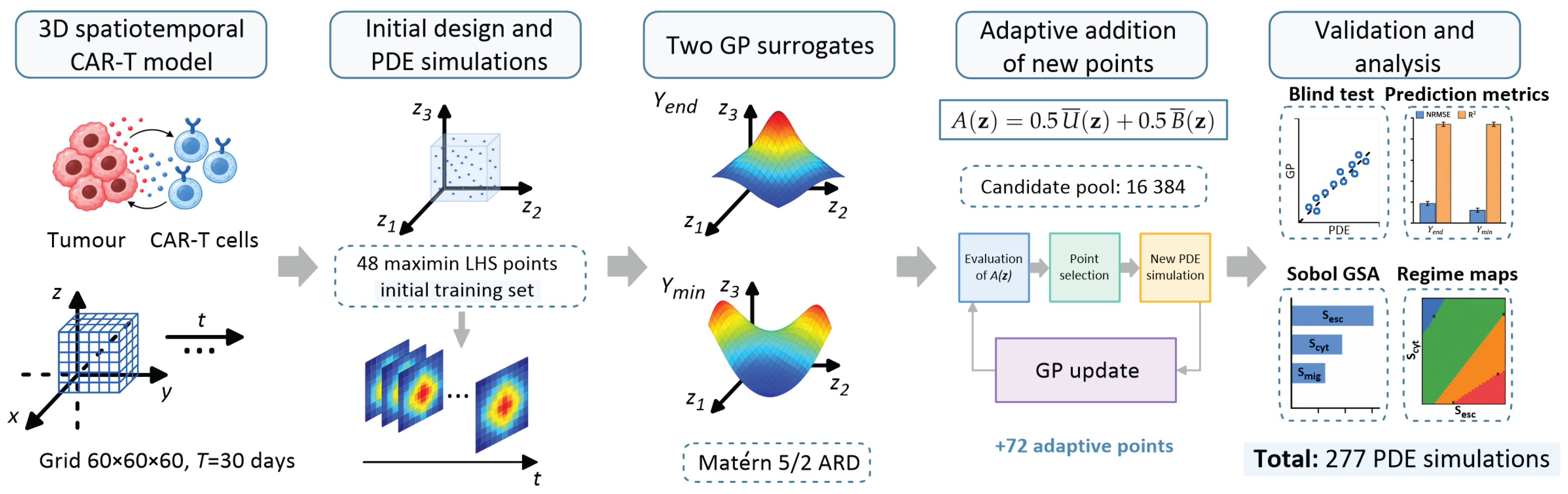
Figure 2.
Representative trajectories of the normalised tumour burden for the four computational response regimes. The reference configuration corresponds to PR; DC, RL, and Failure are shown for comparison. The horizontal dashed line indicates the baseline level . Regime classification is based on and according to rule (8).
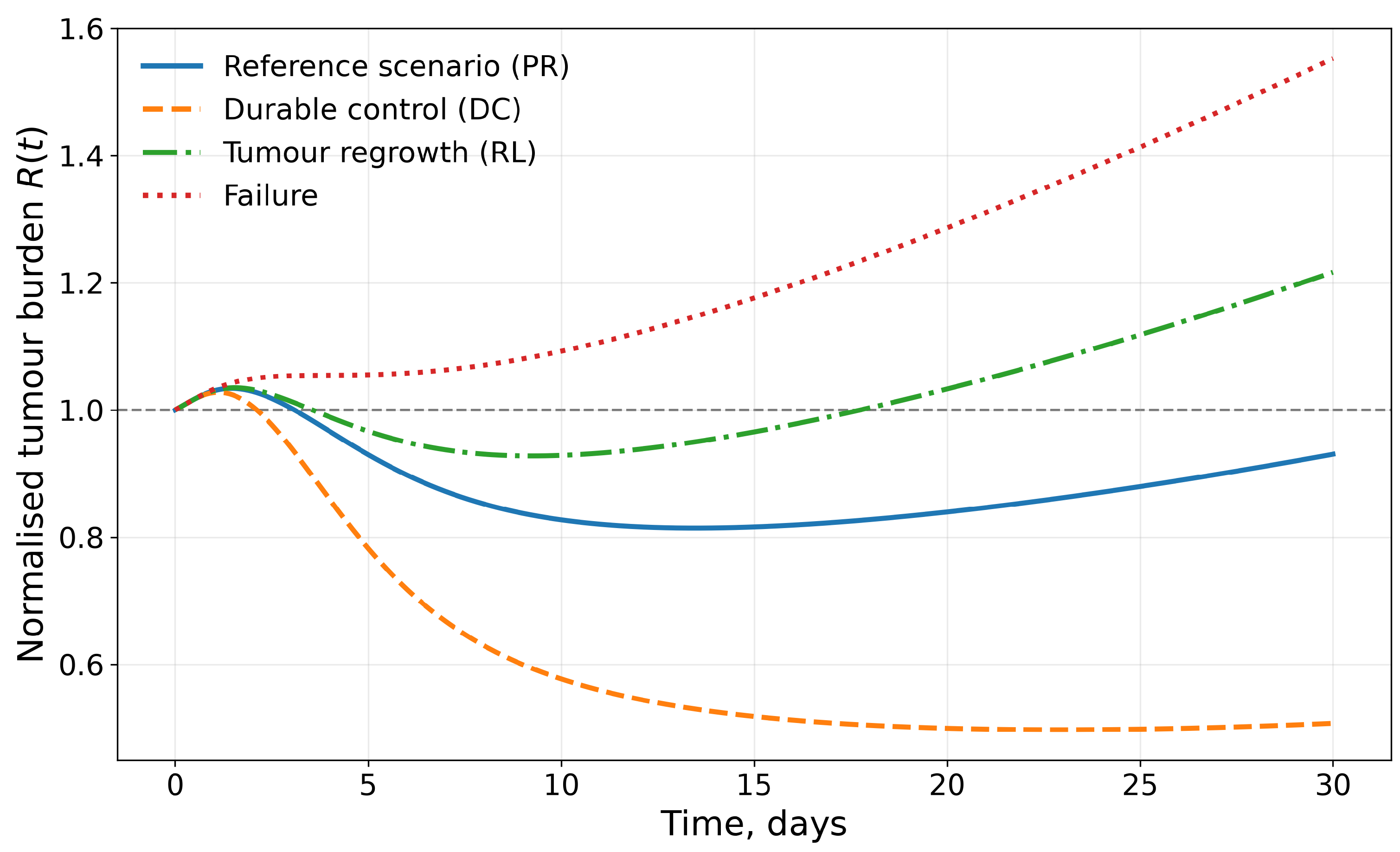
Figure 3.
One-factor change in the final normalised tumour burden relative to the reference configuration, . For each mechanism, simulations at and are shown, with all remaining multipliers fixed at 1. Negative values indicate a reduction and positive values an increase in final tumour burden relative to the reference simulation.
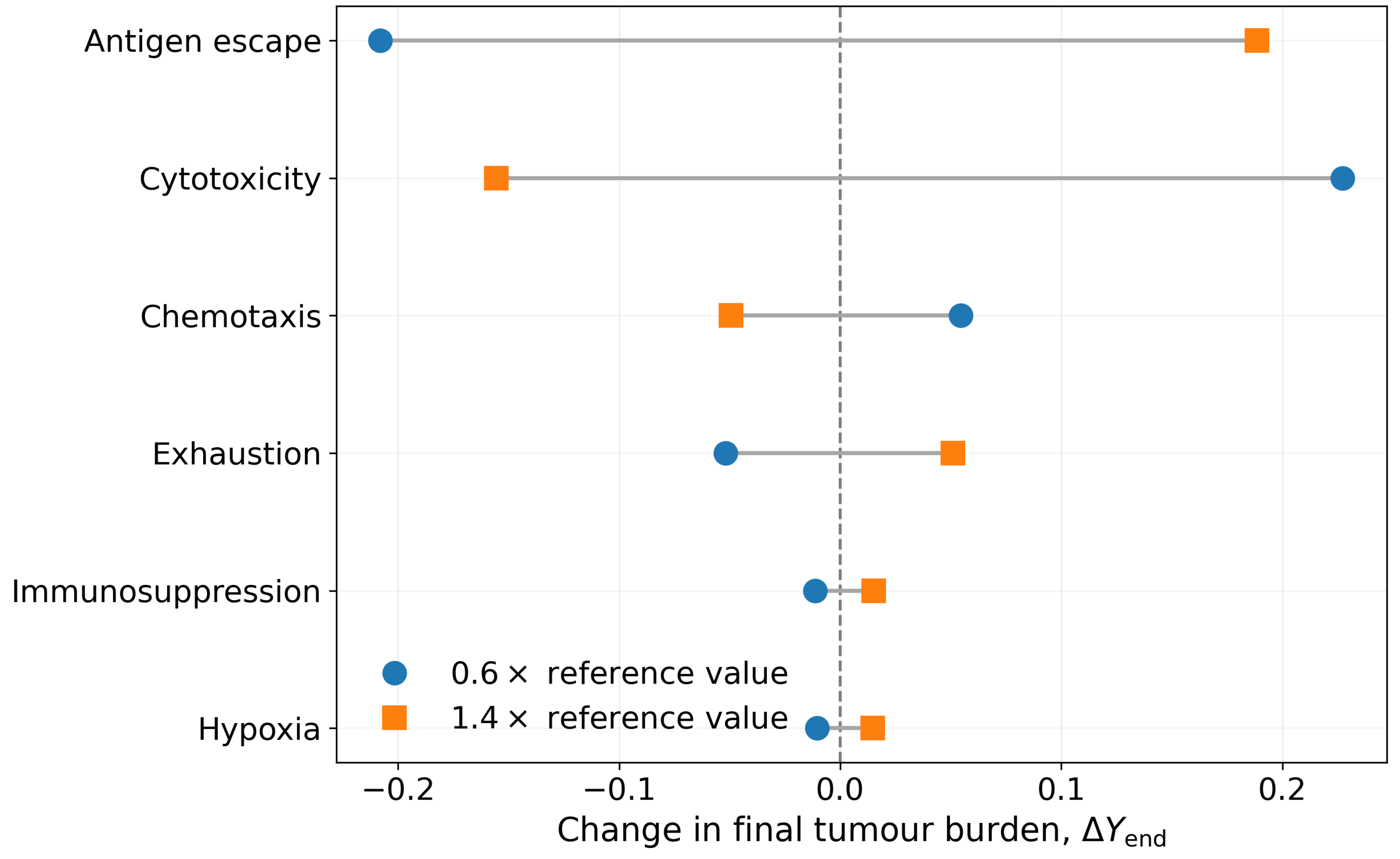
Figure 4.
Comparison between final GP predictions and direct PDE simulations on the fully held-out blind set: (a) final normalised tumour burden ; (b) minimum normalised tumour burden . The dashed diagonal indicates perfect agreement, . The panels report , NRMSE, and coverage of the 95% GP predictive intervals.
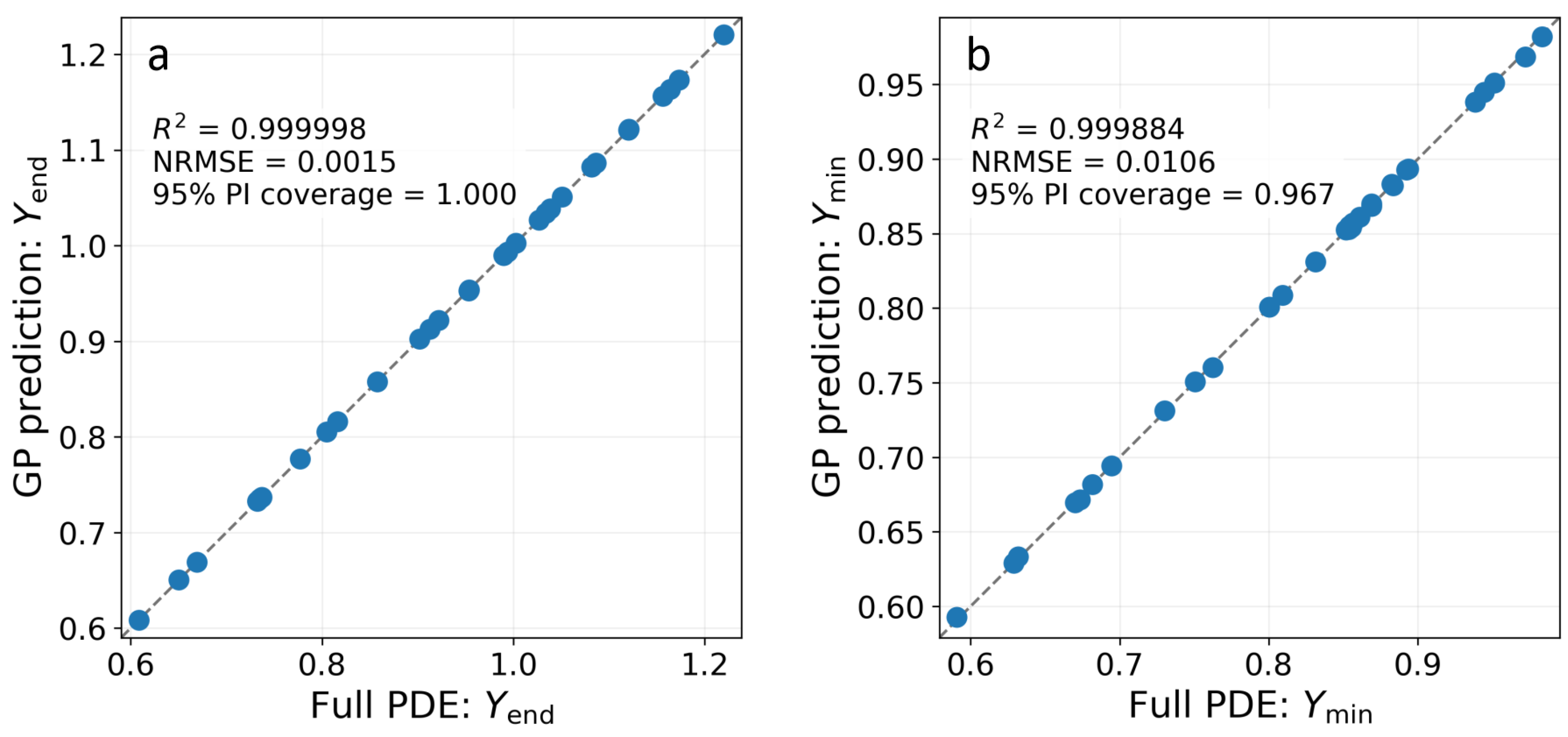
Figure 5.
Comparison of NRMSE for the GP, quadratic regression, and linear regression on the same blind set. Bars correspond to and . All models were trained on the same final adaptive set of 120 PDE simulations.
Figure 5.
Comparison of NRMSE for the GP, quadratic regression, and linear regression on the same blind set. Bars correspond to and . All models were trained on the same final adaptive set of 120 PDE simulations.
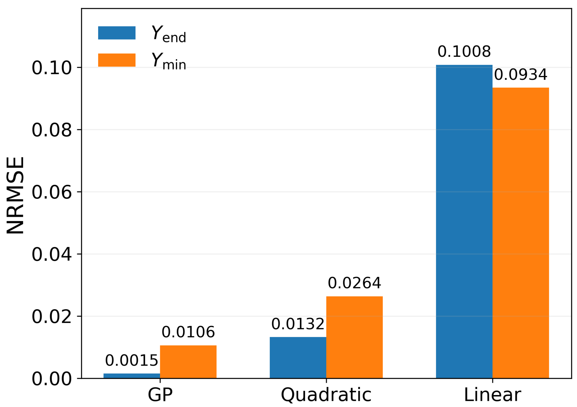
Figure 6.
Comparison of adaptive and non-adaptive space-filling enrichment at the same number of full PDE simulations: (a) NRMSE for ; (b) NRMSE for . Both strategies use the same initial 48-point LHS design. Regime-classification accuracy was 100% for both branches at all checkpoint sample sizes and is not shown.
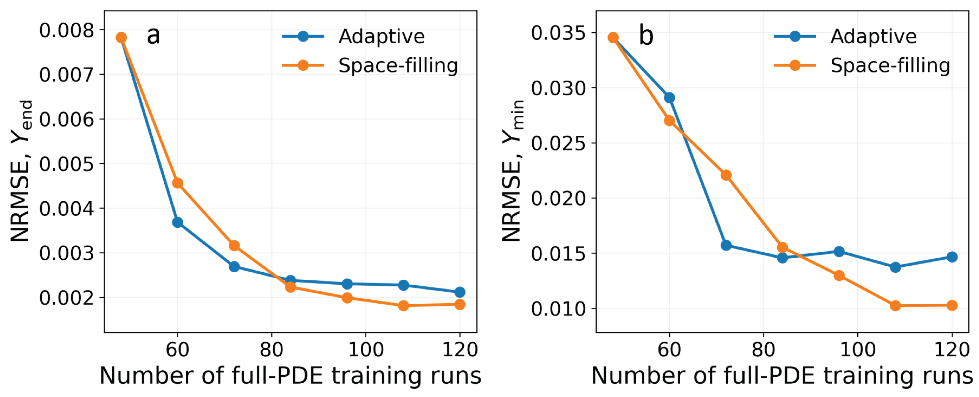
Figure 7.
Projection of the initial LHS design and adaptively added points onto the – plane. The coloured surface shows the final GP prediction of with the remaining mechanisms fixed at their reference values. Open circles denote the initial LHS design, whereas crosses indicate adaptively added PDE simulations.
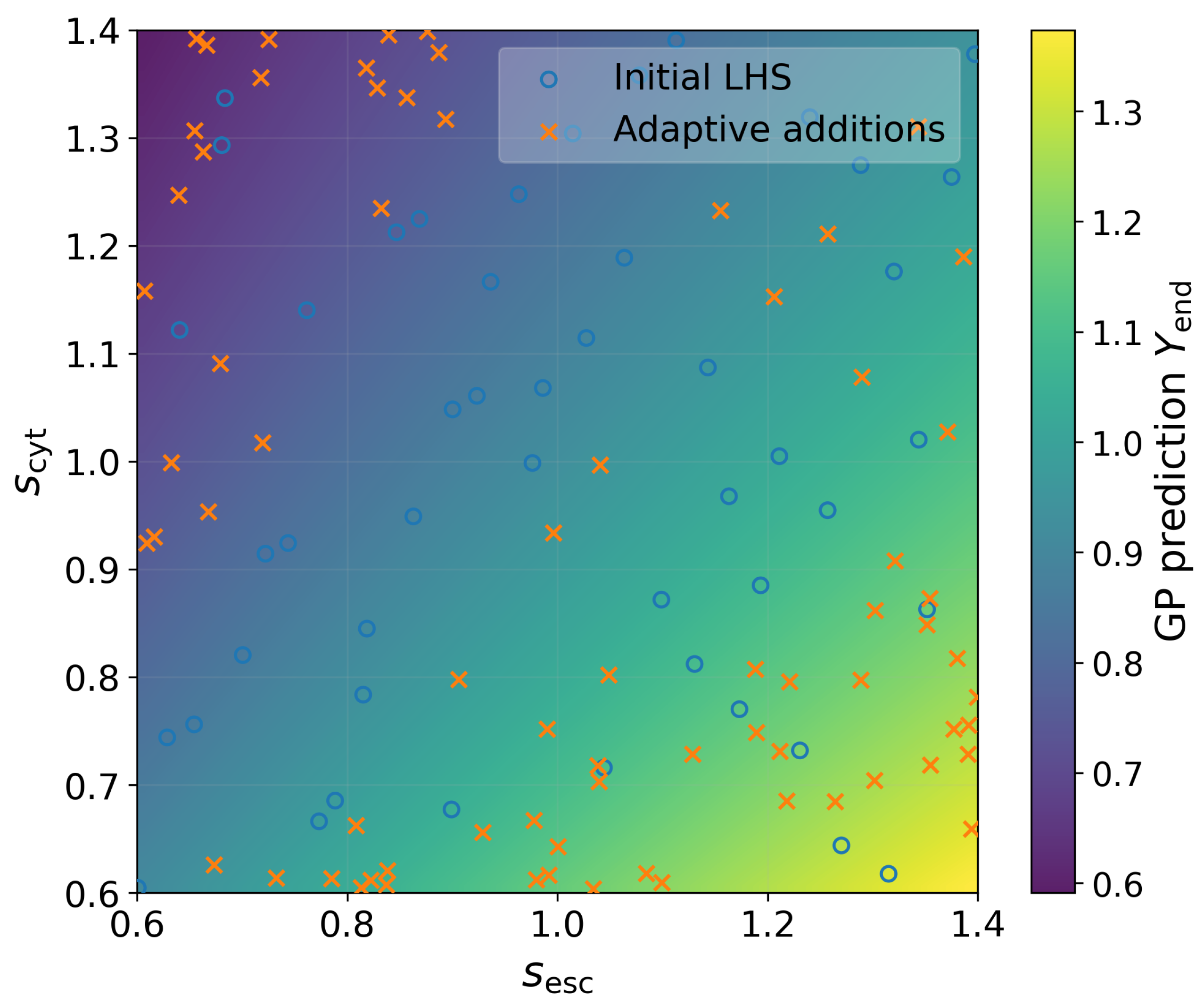
Figure 8.
First-order and total-order Sobol indices for . Mechanisms are ordered by decreasing total-order index; error bars indicate 95% bootstrap intervals.
Figure 8.
First-order and total-order Sobol indices for . Mechanisms are ordered by decreasing total-order index; error bars indicate 95% bootstrap intervals.
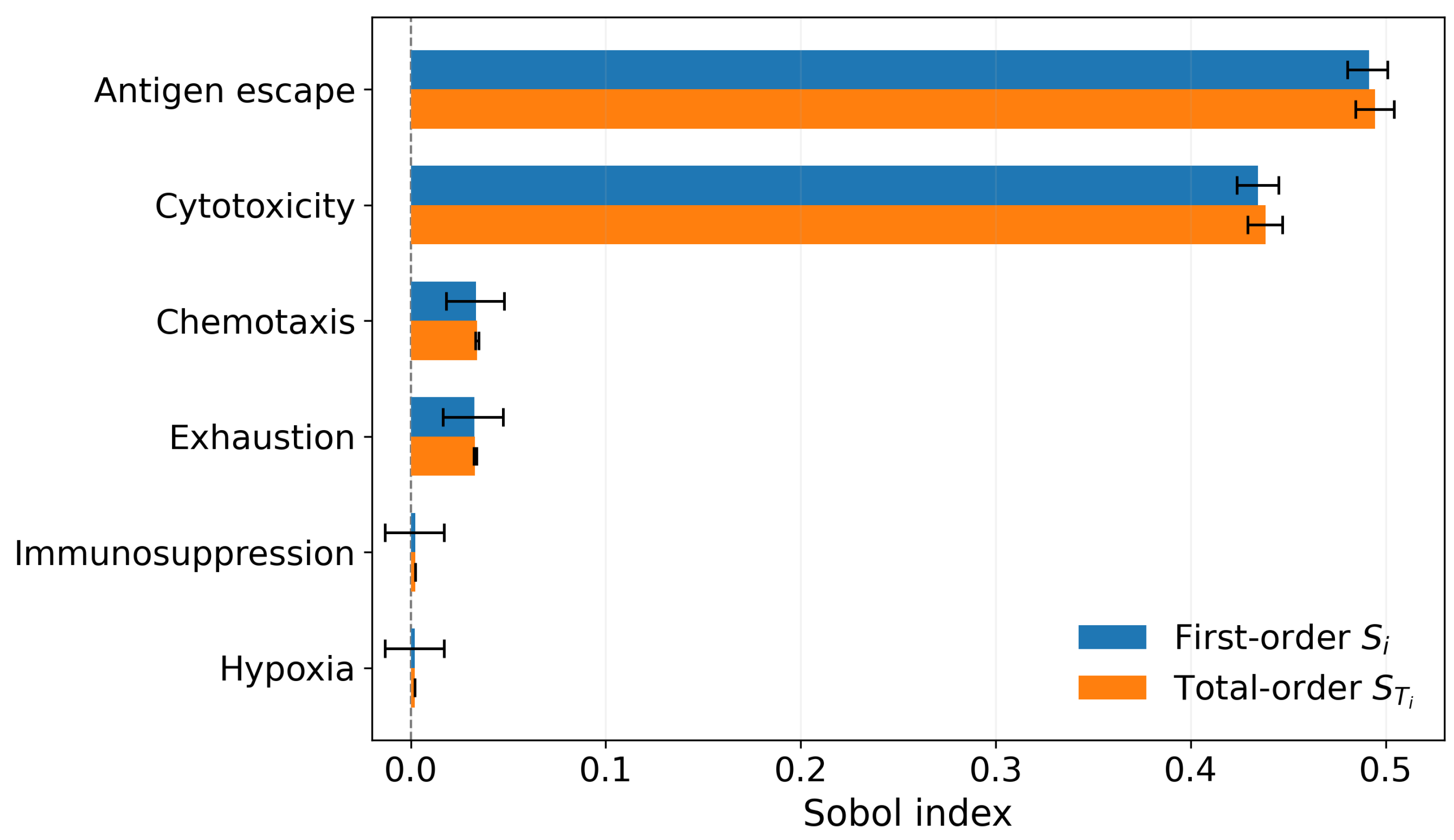
Figure 9.
Pairwise maps of computational response regimes: (a) –; (b) –; (c) –. Mechanisms not shown are fixed at their reference values (). Colours indicate regions corresponding to DC, PR, RL, and Failure; black crosses denote independent direct PDE verification points selected near the GP-predicted regime boundaries.
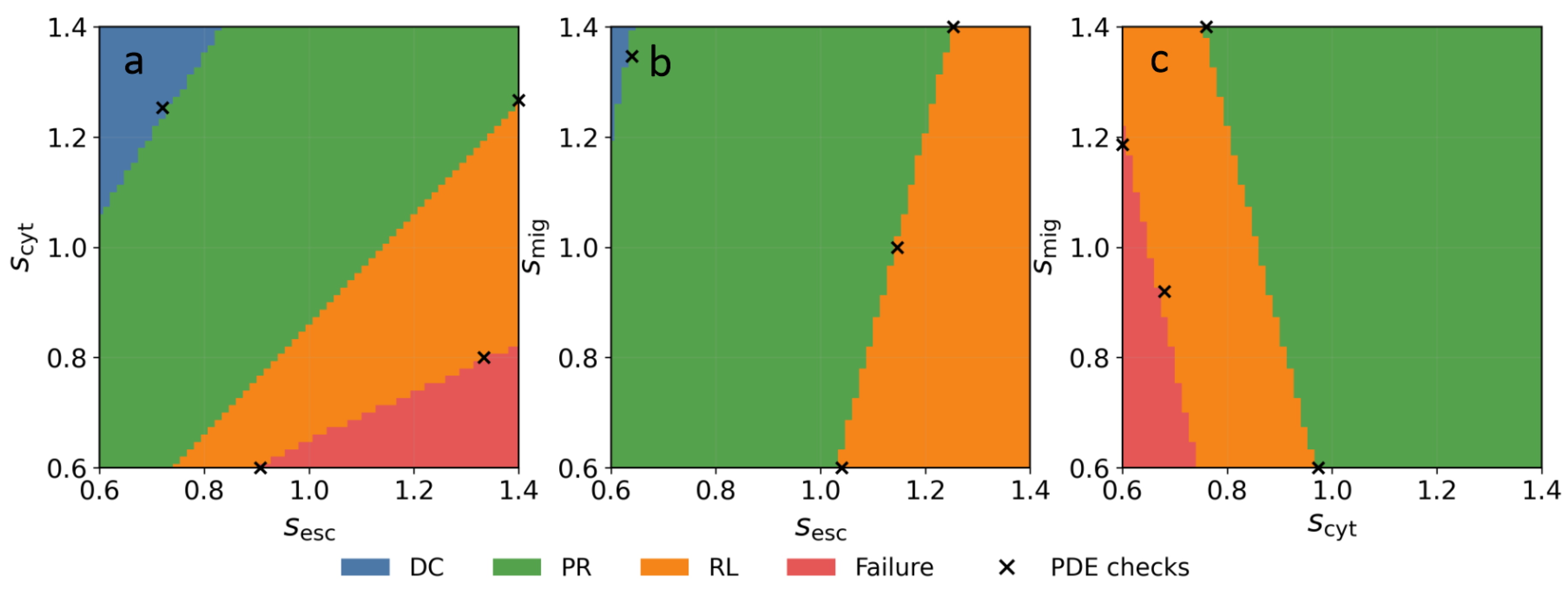

Table 1.
Comparison of surrogate models on the same fully held-out blind set ().
| Model | NRMSE | NRMSE | Regime accuracy |
||
|---|---|---|---|---|---|
| GP | 0.00148 | 0.01058 | 0.999998 | 0.999884 | 1.000 |
| Quadratic regression | 0.01325 | 0.02638 | 0.999818 | 0.999280 | 1.000 |
| Linear regression | 0.10080 | 0.09345 | 0.989489 | 0.990966 | 0.933 |
Table 2.
Sobol indices for with 95% bootstrap intervals.
| Mechanism | 95% interval | 95% interval | ||
|---|---|---|---|---|
| Antigen escape | 0.4913 | 0.4804–0.5008 | 0.4944 | 0.4843–0.5042 |
| Cytotoxicity | 0.4346 | 0.4235–0.4451 | 0.4382 | 0.4291–0.4469 |
| Chemotaxis | 0.0334 | 0.0181–0.0480 | 0.0340 | 0.0332–0.0348 |
| Exhaustion | 0.0327 | 0.0164–0.0473 | 0.0329 | 0.0322–0.0337 |
| Immunosuppression | 0.0022 | –0.0171 | 0.0023 | 0.00227–0.00239 |
| Hypoxia | 0.0021 | –0.0172 | 0.0021 | 0.00209–0.00219 |
Disclaimer/Publisher’s Note: The statements, opinions and data contained in all publications are solely those of the individual author(s) and contributor(s) and not of MDPI and/or the editor(s). MDPI and/or the editor(s) disclaim responsibility for any injury to people or property resulting from any ideas, methods, instructions or products referred to in the content. |
© 2026 by the authors. Licensee MDPI, Basel, Switzerland. This article is an open access article distributed under the terms and conditions of the Creative Commons Attribution (CC BY) license (http://creativecommons.org/licenses/by/4.0/).
Copyright: This open access article is published under a Creative Commons CC BY 4.0 license, which permit the free download, distribution, and reuse, provided that the author and preprint are cited in any reuse.