

Submitted:
13 October 2026
Posted:
14 October 2026
You are already at the latest version
Abstract
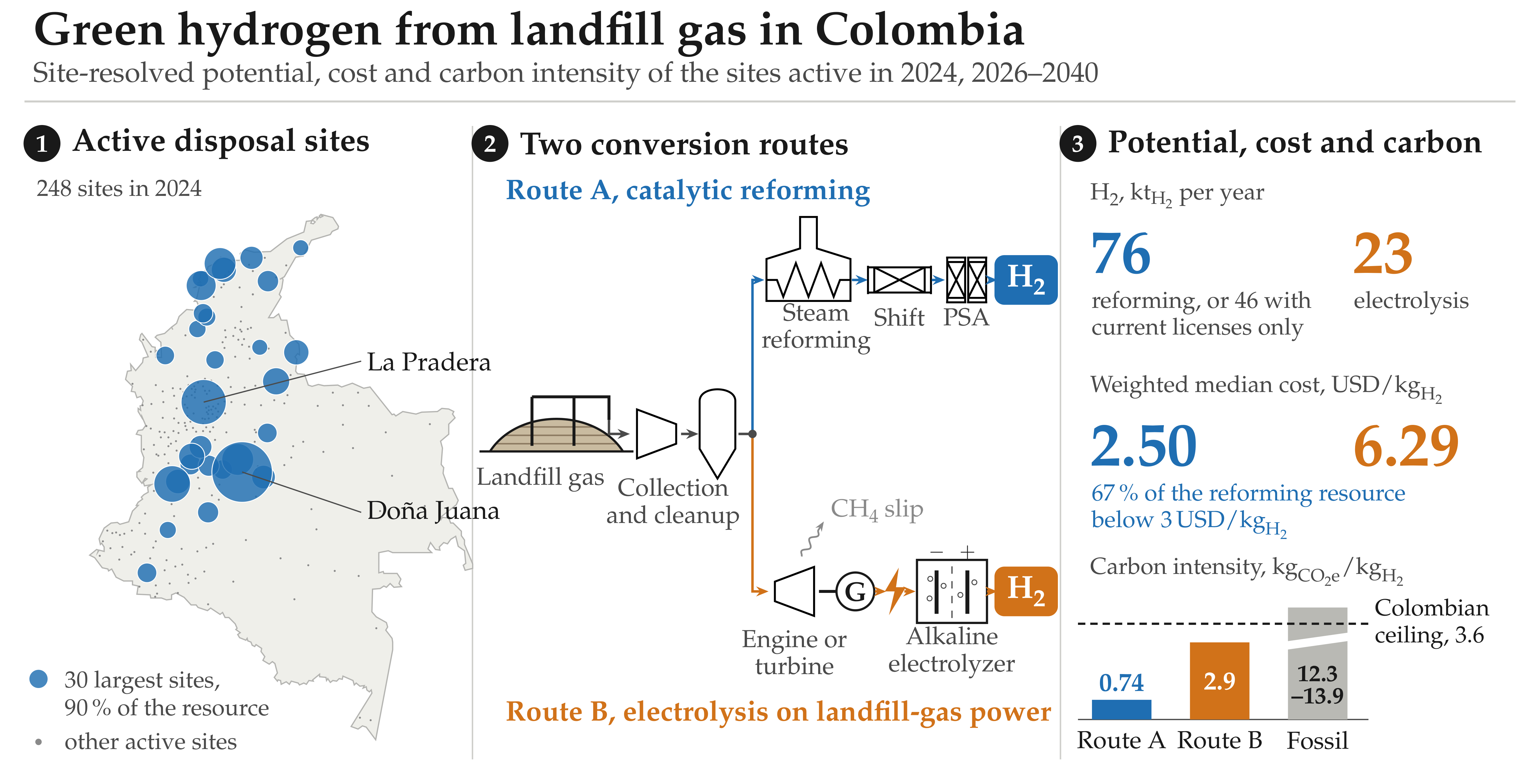
Landfills emit biogenic CH4 with which green H2 can be produced. However, in developing countries, its territorial potential is unknown. This study presents the first site-resolved national assessment of that potential, with cost and carbon intensity, in Colombia. The 248 disposal sites active in 2024 were analyzed. The CH4 emissions were estimated with a first-order decay model according to the recommendations of the Intergovernmental Panel on Climate Change (IPCC) and the United States Environmental Protection Agency (US EPA). Catalytic reforming and electrolysis projects were evaluated, with Monte Carlo propagation. Through reforming, production was estimated at 76\( kt_{H_{2}} \)/yr if these sites keep receiving waste, and at 46\( kt_{H_{2}} \)/yr if they close when the current licenses expire, whereas through electrolysis, production was estimated at up to 23\( kt_{H_{2}} \)/yr. The estimates indicated that 90% of the national potential is concentrated in 30 landfills, and that 67% of the H2 via reforming (23-89%) costs less than 3USD/\( kt_{H_{2}} \). The CH4 slip proved decisive for the carbon intensity, 0.74\( kg_{CO_2}e \)/\( kt_{H_{2}} \) for reforming and 2.9\( kg_{CO_2}e \)/\( kt_{H_{2}} \) for electrolysis. Capturing the biogenic CO2 generated in reforming would reduce its carbon intensity to -4.1\( kg_{CO_2}e \)/\( kt_{H_{2}} \), provided that the transport and storage of CO2 exist.
Keywords:
green hydrogen
; landfill gas
; municipal solid waste
; biogenic methane
; steam reforming
; water electrolysis
; methane slip
; levelized cost of hydrogen
; carbon intensity
; Colombia
1. Introduction
Green H2 holds a central place in the decarbonization strategies of nations, as a fuel and feedstock, whose oxidation produces only H2O [1,2], and research on its production has focused mainly on electrolysis with solar and wind energy [3,4]. Less attention has gone to the CH4 that is emitted at landfills as a renewable and carbon-bearing feedstock that is generated in almost every city, and that abounds in the Global South [5,6]. However, only a small fraction of the municipal solid waste (MSW) generated worldwide reaches landfills capable of capturing their landfill gas (LFG), composed mainly of CH4 (4060), and much of the LFG captured is burned in flares to reduce its impact on global warming [5,7].
Because the carbon contained in LFG is biogenic, the H2 produced from it can be counted as renewable [8], and classified as green, including under Colombian law [9]. Among multiple routes that can be used to convert LFG to H2 (LFGtH2), there are direct reforming and its use as engine fuel to generate the electricity required by electrolyzers, two routes that differ in H2 yield, in capital cost (CAPEX) [10,11] and greenhouse gas (GHG) emissions, which, in the case of reforming, arise from the CH4 slip that engines and upgrading units let escape [12]. Nevertheless, the thresholds of the European Union (EU) and of Colombia admit this H2 if that CH4 slip is kept relatively low [13], and at a maximum of 0.13CH4/H2 in the case of Colombia [14].
Techno-economic analyses of LFGtH2 projects have mainly examined European cases [15,16], while for Colombia and other developing countries the energy assessments of MSW at the national or municipal scale have omitted H2 [17,18,19]. Few estimates extend to H2 at the national level. One of them, for the United States, counted the landfills, but the cost was omitted [20]. Another, a global mapping, estimated the price of H2 from the gasification of MSW at nine landfills [21], and a costing of CH4 reforming across Brazil reported the avoided emissions of the total potential and not the carbon intensity (CI) of each site [22], but, to date, no assessment has resolved site by site the LFGtH2 potential of a developing country with cost and CI, and none has asked what part of the resource depends on extending the useful life of each landfill.
In this context, Colombia offers favorable conditions to answer these questions, given that its sanitary landfills receive 96.7 of the MSW disposed of [23] and it has public records of the flows to each site from each municipality. In that sense, this study aimed to assess the production of green H2 from projected LFG emissions in Colombia between 2026 and 2040, estimating these emissions using as a basis the sites active in 2024, which concentrate 97.9 of the potential (the remaining 2.1 corresponds to more than 1600 closed sites), analyzing two LFGtH2 routes, one by direct catalytic reforming, and the other by electrolyzers powered by engines that burn the LFG.
For each site, the study estimated the technical potential of H2, its levelized cost (LCOH) and its cradle-to-gate CI, including a variant with carbon capture that took the reforming route to negative emissions. In this way, it was investigated how much green H2 each route could supply, how much depends on deposits after the expiration of the current licenses, how the potential and the LCOH are distributed among the sites, whether, once the CO2e emissions are counted, the green H2 generated meets the emission limit allowed by Colombian regulations, and which route suits each site. Unlike a resource inventory, this assessment differentiated between the potential obtained under the current licenses and the part that depends on their extensions, because half of the MSW disposed of in 2024 was taken to sites whose licenses had already expired or will expire at the latest in 2027.
2. Literature Review
2.1. LFG and Its LFGtH2 Routes
According to global inventories, about 70 of the MSW collected ends up in sanitary landfills and open dumps [5,24], and in developing nations sanitary landfilling remains the main method because it is perceived as cheap and operationally simple [25], while open dumps predominate outside the areas of influence of sanitary landfills [24,26]. The decomposition of MSW makes landfills the third-largest anthropogenic source of CH4 worldwide [27]. Nevertheless, only about 8 of the world’s MSW went to landfills with LFG capture in 2016 [5]. LFG-to-energy (LFGtE) projects are rarely profitable, especially without subsidies [7]. Because plants took the carbon of LFG from the atmosphere recently, the CO2 released in its conversion is not counted as a GHG, while the CH4 that escapes is [7,28,29].
Steam reforming is the most widely used commercial process for biogas and LFG, offers the highest H2 yield per mole of CH4 and has reached technology readiness level (TRL) 9, while partial oxidation and autothermal reforming are still immature for this feedstock [8]. Autothermal, membrane and sorption-enhanced variants add purity or integration, but also complexity, and none is documented at landfill scale [30,31,32]. Because the reaction is endothermic, about 1.42.1LFG are required per f feed to supply heat [8], which implies that only 3242 of the captured LFG enters the reforming route, while the remaining 5868 is used to meet the energy requirements of the process.
Moreover, reforming also requires a feed free of siloxanes and hydrogen sulfide (H2S), since they deactivate the catalysts used [8,33,34,35,36]. Indeed, even traces of H2S poison the active nickel phase (Ni0) of the heterogeneous catalyst on which the chemical reaction occurs, through irreversible chemisorption on its active sites, so the feed stream must guarantee a concentration below 20ppm [8]. Halogenated, aromatic and organic sulfur traces [27] and chlorinated hydrocarbons in the condensate [24] add to the contaminant load, and catalyst life depends more on the cleanup of the LFG than on the reformer itself [37]. This cleanup, and the upgrading of the LFG, consume electricity [38], and the latter also loses 0.12 of the CH4 it processes [12,38,39].
On the other hand, the electrolysis route burns the LFG in engines or turbines to power an electrolyzer. Electrolysis dominates H2 strategies because its cost decreases with that of renewable electricity [40,41], and both alkaline (ALK) and proton-exchange membrane (PEM) units have reached TRL 9 [42]. CH4 slip amounts to about 0.02 in gas turbines, and up to 0.43.3 in reciprocating engines [12,43,44,45]. Both types of electrolyzer, ALK and PEM, have a similar specific consumption [46,47]. However, ALK units are cheaper, last longer and adapt to stable loads, while PEM units adapt to rapid load changes [48,49,50,51,52]. Solid oxide (SOEC) and anion-exchange membrane (AEM) units, for their part, remain costly or are at the demonstration stage [42,53].
In tropical developing economies such as Colombia, studies have optimized electrolysis for photovoltaic supply, favoring the use of PEM electrolyzers [54,55,56], but with naturally intermittent energy supplies, which markedly reduces their net capacity factor, and exposes the sector to grid-connected systems, where costing and dispatch occur under conditions different from those of isolated systems [57]. A sanitary landfill, in contrast, supplies LFG continuously. With respect to the water footprint, electrolysis consumes about 12H2O/H2 [58,59], representing a threat to the water resources of tropical populations affected by phenomena such as El Niño.
2.2. Cost of H2 from Biogenic CH4
Cost studies of biogas reforming range from compact pilot-scale units to plants on the order of tens of metric tons per day [60,61,62,63,64,65]. Nevertheless, no study concerns a developing country. At the national scale, Przybyla et al. [22] estimated the LCOH of reforming the CH4 of LFG in Brazil, identifying 204 sites below 10/H2, and 33 below 5/H2, demonstrating an inversely proportional relationship between the LCOH and the rate at which the landfill receives MSW. However, the investment was amortized over a remaining life derived from a nominal life of 30 years for all landfills.
Regarding the CAPEX of a plant, scaling exponents differ depending on the study and the scale [66,67,68,69], while those of the reforming train cluster between 0.60 and 0.75 [60,70]. Reformer CAPEX values available in the literature cover plants from about 100H2/day to more than 600H2/day, with varied scopes (i.e., equipment, installed cost or total-plant cost) [60,71,72,73,74,75,76,77], while overall efficiency varies between 0.60, for distributed units, and 0.76, for central plants [78,79,80,81,82]. A plant cost index and the cost-capacity relation make those records comparable [83,84].
Likewise, electrolyzer estimates that include only the equipment represent about half of the CAPEX of plants with detailed engineering [46,48,49,85,86,87], and fitted exponents differ between unit operations [88,89]. The LCOH [90] inherits this dispersion, which Monte Carlo simulation propagates [58,91], while partial rank correlation ranks the input variables that determine this dispersion [92].
2.3. Carbon Accounting and Certification
Given that EU rules classify H2 from biogas as a renewable fuel obtained from biomass and not as a renewable fuel of non-biological origin [13], and that no internationally agreed terminology exists [8], certification schemes judge H2 by its emissions at the production gate [93,94,95]. The EU requires a fixed fraction of savings against a fossil comparator, equivalent to 3.383.95CO2e/H2 [13,96,97], and in 2026 Colombia set a cradle-to-gate ceiling of 3.6CO2e/H2 for the H2 produced to be considered low-emission [14]. It is worth highlighting that, in this work, the term “green H2”, although compatible with EU regulations, is confined to Colombian law.
Life-cycle studies suggest, for H2 of fossil origin without carbon capture, a CI of 12.313.9CO2e/H2 [98], while with carbon capture, this CI depends mainly on CH4 emissions, on the capture rate and on the warming metric [99]. For its part, H2 obtained from biogas reforming reaches 4.87.5CO2e/H2, with dry reforming of biogas or biomethane, and up to 10.8CO2e/H2 with chemical-looping dry reforming, all above the EU and Colombian thresholds [8].
From that perspective, for biogenic feedstocks the decisive term is CH4 and not CO2, since the former, although not of fossil origin, has a global warming potential (GWP) 27 times higher than the latter, over a horizon of 100, according to the Sixth Assessment Report of the Intergovernmental Panel on Climate Change (IPCC) [100], and 28 times higher according to its Fifth Assessment Report [101]. Even so, the default values of inventories and the life-cycle models of sanitary landfills assume that engines and flares destroy almost all the CH4 that is generated within the site [102,103], although it is proven that the losses measured at biogas plants are significant [12], and therefore, CH4 losses along biogas supply chains are usually underestimated [104].
In the case of carbon capture, reforming concentrates the carbon of its feed in a stream from the shift section at high partial pressure, while the burner releases a dilute flue gas whose separation is more costly [105], and the storage of that biogenic carbon generates negative emissions [106,107]. Capture costs vary with streams and scale [81,108,109,110], solvent regeneration adds heat demand [108,110,111], and transport and storage cost more for an isolated source than for a shared hub [112,113,114,115].
2.4. Resource Assessments, Generation Models and Spatial Methods
In Colombia, energy assessments of MSW have quantified the electricity and the CH4 that large sanitary landfills could deliver [17,116,117]. Other studies report electricity for countries, regions or large cities [18,19,26,118], or else rely on aggregate statistics and on default or unreported generation parameters [18,19].
In Brazil, where few sanitary landfills recover energy [119], the electric generation capacity of the landfills in operation was estimated spatially [120]. Rueda-Avellaneda et al. [121] assessed the LFG of the 198 sanitary landfills of Mexico for electricity, industrial fuel and compressed biomethane. H2 was omitted mainly for lack of a regulatory framework. Process studies, in contrast, have addressed biogas reforming, considering generic compositions without trace contaminants [10,79,122,123].
For CH4 generation, first-order decay models such as LandGEM and its Latin American derivatives are widely applied [27,124,125,126,127], although their single-parameter form poorly describes the fast-degrading waste of the humid tropics [128,129]. Data taken in the field and from reports also yield higher decay constants in wetter climates [128,130] than the default values established by the United States Environmental Protection Agency (US EPA) [131]. Parameters can be transferred between models [132] or taken from inventory guidelines [133]. Nevertheless, uncalibrated default values are biased relative to measured recovery [134,135]. A recent review found that numerical models of sanitary landfills, mostly first-order, rarely translate CH4 into recoverable energy [136]. Additionally, although LFG generation persists after the closure of the site, it decreases abruptly after closure [27].
As for LFG collection, efficiencies of 50100 are reported depending on the type of landfill cover and the coverage of the well field, and they are high only under an impermeable final cover, which can take years to implement [27]. This makes collection efficiency the most uncertain input variable, with in situ measurements of 41 under daily cover and about 70 under intermediate and final covers [137]. Indeed, recent measurements report less than models and guidelines assume [125,138,139]. Thus, given that the uncertainty affects all collection fields equally, collection efficiency is not extrapolable between sites [140]. Semi-controlled cells and open dumps retain much less LFG [24,26,139,141,142]. Even so, assessments usually fix the efficiency at a single value (e.g., 75) [19,29,103], although it determines the recoverable energy and the position of sanitary landfilling relative to other treatments [143].
The composition of MSW is much more complex to predict than the generation of MSW itself [144], while global inventories stratify it by income level [5,145]. In Colombia, although the socioeconomic stratum is an indicator related to composition [146,147], the quality of municipal characterizations varies markedly with the administrative capacity of site operators [148,149]. However, high organic fractions can be associated with small and intermediate cities with low economic development [150].
Beyond individual plants, geospatial models have been applied to biogas and renewable H2 [56,151,152], location models to biogas plants [153] and supply-cost curves to distributed renewable resources [154]. A national estimate of renewable H2 from biogas in the United States analyzed the sanitary landfills one by one [20], but it was limited to estimating the technical potential.
The global geospatial model of Alrbai et al. [21] covers more than 9000 sanitary landfills, with a neural network for the organic fraction. Its H2 comes from gasifying the MSW and not from reforming the LFG, its price is estimated only at three sites in each of China, India and the United States, and its emissions are counted as displaced grid electricity. These tools come mostly from high-income contexts, whose designs may not be attainable elsewhere [5,6,27,155].
2.5. The Colombian Context
In the more than 1100 municipalities of Colombia, the sanitary landfill is the sole legally authorized final disposal system, accompanied only by marginal transitional and contingency cells, and unauthorized dumps, and it received 96.7 of the MSW disposed of in 2024 [23]. The regulator, the Superintendency of Residential Public Services of Colombia (SSPD), publishes every year what is disposed of at each site, which municipality it comes from, and the remaining useful life of each site [23,156], a near-complete census that contrasts with the scarcity of data that limits estimates in countries such as India, Nigeria, Ghana and Bangladesh [18,19,26,118]. The integrated management of MSW and its recovery have been national policy for a decade [157,158]. The Mining and Energy Planning Unit of Colombia (UPME) studied the energy potential of MSW, managing to determine departmental characterizations of MSW [159].
Additionally, in terms of the availability and accessibility of the data needed for the estimates of CH4 emissions from the landfills of Colombia, the integrated MSW management plans (PGIRS) can be found, which report measured characterizations, at the source or at the site, for the main cities of the country [160,161,162,163,164,165,166,167,168,169,170,171,172,173,174,175,176,177,178,179,180,181,182,183,184,185,186,187,188,189,190,191,192,193,194,195,196,197,198,199,200,201,202,203,204,205,206,207,208,209,210,211,212,213,214,215]. SSPD inspections document LFG collection at the largest sanitary landfills [216,217,218,219]. The operator of the largest site, “Doña Juana” (Bogotá), publishes its metered LFG flow [220], which it uses for energy. The documents of the Clean Development Mechanism projects that several landfills registered between 2009 and 2017 record when each site opened [221,222,223,224,225,226,227,228,229,230,231,232], as the local press does for the sanitary landfill “El Carrasco” (Bucaramanga) [233]. Population projections, climate normals, municipal boundaries [234,235,236], electricity prices in the wholesale market and grid emission factors [237,238] complete the data.
Likewise, the 2020 climate contribution of Colombia included LFG capture and energy recovery among its measures for MSW, in particular at “Doña Juana”, with an LFG treatment rate of 2 and an expected energy recovery of 0.6 of the LFG produced by 2030 [7]. In Latin America, where the sanitary landfill also predominates and H2 policies are emerging [119,155,239,240], most of those contributions address the improvement of landfills and many include LFG capture [7]. In Colombia, it has been demonstrated that the MSW disposed of in sanitary landfills has not decoupled from income [241]. Therefore, the resource should persist unless organic waste is diverted on a large scale.
Currently, the H2 roadmap sets a target of 13 of electrolysis by 2030 and an LCOH close to 1.7/H2 in the zones with the best renewable resource [242]. However, assessments of that agenda have concentrated on solar and wind energy [55,56,243], while the generation mix that backs grid-connected electrolysis is changing [244]. None has asked whether the country’s own MSW could complement the electrolysis program and to what extent. Although the roadmap calls for storage sites for captured CO2 [242] and the energy transition law orders the government to regulate geological storage [9], this regulation remains pending and no transport or storage infrastructure exists yet [245,246].
3. Materials and Methods
This section expresses quantities in SI units, with gas volumes at 15∘ and 101.325, unless otherwise indicated. The cost correlations of the LFGcost-Web tool of the US EPA [11] were converted to SI units, and all monetary values were escalated to the same reference year (see Section 3.13). The workflow was implemented in Python 3.11 with pandas 3.0, NumPy 2.4, statsmodels 0.15, SciPy 1.17, GeoPandas 1.1 and Matplotlib 3.10.
3.1. Modeling Framework
The analysis of this study was addressed through a geospatial approach that harmonized the national disposal registry into a catalog of sites, reconstructing their deposits from 1985 to 2040 and estimating the recoverable CH4. The recovered LFG fed the two green LFGtH2 routes, catalytic reforming (Route A) and electrolysis with electricity generated from LFG (Route B). The LCOH and the CI of both were calculated site by site. The cradle-to-gate boundary extended from the deposited MSW, excluding collection and transport because they occur with or without LFG utilization, to the H2 outlet. It was considered that the reformer is fed at about 3 for its adsorption unit [8], and the ALK electrolyzer was taken as a pressurized design that delivers up to 3 [49]. In this way, neither route was charged for compressing its product. Additional compression, storage and distribution remained outside the boundary, as in certification schemes [93,94,95].
3.2. Study Area, Disposal Sites and Their Status
The study covered all of Colombia, including the San Andrés archipelago, and its 1104 municipalities reporting disposal. For each year from 2010 to 2024, the regulator published the mass that each municipality delivered to each disposal site, the site class and the expiry of its permit [23,156], in 17321 municipality-site-year records with positive mass. The unit of analysis was the site, and the same site could appear under several spellings, or under the code and the department of the municipality served. The 2377 combinations of name and code were harmonized into 1868 sites through name normalization and the merging, with explicit rules, of the variants of large regional sites. A name registered under several codes of the same department was assigned to its dominant code when this code concentrated at least 70 of the name’s mass. Generic names kept the code under which they were registered.
The sites that received MSW in 2024 were classified as active and the rest as closed. For the active sites, the licensed end of life was the date reported by the operator in 2024. The remaining life was counted from 1 January 2026, the start of the window. The licenses whose expiry was prior to that date were considered expired.
Regarding the scope, only the 248 active sites, which received all the MSW disposed of in 2024, were assessed. The 1620 closed sites were passed through the chain only to estimate their remaining generation, which was 2.1 of the Route A potential of the registry (1.92.3). Most closed a decade or more before the window, and their rapidly degrading waste already exhausted a good part of its CH4 generation potential.
The sites were located at the representative point of their host municipality. The opening years were taken from the Clean Development Mechanism documents for 15 of the largest sites [221,222,223,224,225,226,227,228,229,230,231,232], from the local press for “El Carrasco” [233] and from the site register of the SSPD [156], which together document 108 active sites. The sites that appeared for the first time after 2010 were assigned that year as their opening year.
3.3. Deposits by Site and Year
An evaluation window of 15 years, between 2026 and 2040, was established, for which the disposal of MSW was projected with Equations (1) and ()
where is the mass disposed of by municipality m in year y, in is its urban population and is its per-capita MSW disposal rate in the reference years . The same Equation (1) was used to back-cast missing observations. was kept constant considering the recently reported evidence for the same municipalities, which suggests that it is not possible to establish a decoupling between the disposal of MSW in landfills and the income of the municipalities [241]. The population was taken from the official projections of the National Administrative Department of Statistics (DANE) [234].
The projected mass was allocated with the delivery shares of the municipality in 2024, and the back-cast mass with those of its first observed year, starting from the opening year of the site, with a cutoff in 1985, or in 1995 if that year was not documented. Earlier MSW went to unrecorded predecessor open dumps. That MSW was excluded (39.6MSW between 1995 and 2009). The gaps within the registry, mostly from 2015 to 2017, were filled by interpolating the municipality’s own mass, which added 1.18MSW in total.
For the base case, it was considered that the active sites would keep receiving MSW throughout the evaluation window, as the 54 active sites with an expired license did in 2024. Under this assumption, 62 of the mass projected up to 2040 fell after the licensed end of life. For this reason, each projected deposit was split at the licensed date into a licensed layer and a beyond-license layer, with the expired licenses cut at the start of the window and the missing dates filled with the median remaining life of their class. A licensed-only variant discarded the second layer.
A diversion variant removed a fraction of the two fastest decay categories (Section 3.5), the food and garden waste. It was assumed that this fraction grew linearly from 5 in 2026 to 50 in 2035 and remained constant until 2040. Since these categories represented 59 of the deposits of 2024, the full level removed 30 of the MSW. It was applied equally to the base case and to the licensed-only case.
Since decay constants depend on moisture, each site was assigned to one of the five precipitation zones of the Colombia Landfill Gas Model [125]. Each site was assigned the inverse-distance-weighted mean of the 1991–2020 normals that the Institute of Hydrology, Meteorology and Environmental Studies (IDEAM) publishes for 1599 stations [235], within 25, or in a larger radius where there was no station within that radius. The station of the largest site records 672/, in zone Z4 (Section 3.5).
3.4. Input Data
Table 1 presents the datasets used and their role.
3.5. Estimation of CH4 Emissions
LFG generation was estimated with the first-order decay model of the Colombia Landfill Gas Model [125] and of its Mexican antecedent [126]. With this model, the MSW of each year of disposal was divided into four decay categories. Each one has its own decay constant and its own potential capacity. With Equations (3) and (), the CH4 of year t was summed over the decay categories, the years of disposal and the 10 equal parts of each deposit, each one located at the middle of its tenth of a year and with generation starting after the six-month lag of the Colombian model [125]. The rate was evaluated at mid-year
where represents the CH4 rate in c, j and m index the categories, the years of disposal and the tenths of a year, respectively; , in and , in are the decay constant and the potential capacity of category c, respectively; denotes the mass fraction of category c in the MSW of year ; is that MSW mass in is the CH4 correction factor of the site class; is the time elapsed since tenth m began to generate; and is the half-year lag. Only the parts whose was not negative were summed. Setting the lag to zero or to one year changed the national generation by 0.8 within the evaluation window.
The LFG flow was determined using Equation (5), where is the total LFG flow in and is its CH4 volume fraction.
Table 2 presents the capacities and the decay constants by precipitation zone of the Colombian model [125]. The capacity of category 2 was set near the midpoint of its reported range of 93134CH4/MSW. The mass fractions were derived as described in Section 3.6. The model was checked against the only metered collection field in the country (see Section 3.16).
Table presents the gas properties and the constants of both routes, with the GWP of non-fossil CH4 taken from the Sixth Assessment Report of the IPCC [100]. The values of the Fifth Assessment Report of the IPCC [101], 28 without climate-carbon feedback and 34 with it, were used as sensitivity cases.
3.6. MSW Composition by Site
Equation (3) requires the composition of the mixture that arrives at each site, which may combine the MSW of dozens of municipalities. For this reason, the composition was resolved first by municipality.
The characterization reported in the PGIRS of the municipalities was used when it was available, which occurred in 56 municipalities (see Table S3 of the Supplementary Materials) [157,158]. When a PGIRS reported characterizations at the source and at the disposal site, the one at the site was taken. For the cases in which a municipality did not report a characterization in its PGIRS, it was assigned the departmental average of the national waste-to-energy assessment, compiled from the regulatory reports of the 32 departments and the Capital District [159]. Since this assessment covers all departments, in no case was it necessary to resort to a national average.
Table 3 shows the 10 commercial categories of the departmental profiles reported by the UPME [159] with their decay categories. Food was reported together with other rapidly degrading organics.
The mixture that each site receives was obtained with Equation (6), where and represent the mass fractions of category c at site s in year t and in the MSW of municipality m; and is the mass that m sends to s in year t.
Then, the capacity of the site was obtained using Equation (7), where is the weighted potential capacity of the mixture at site s in year t, in
As a cross-check, Equations (8) and () were used to estimate the degradable organic carbon (DOC) and the capacity that it implies according to the national inventory guidelines of the IPCC [131,133]
where is in and are the mass fraction and the default carbon content of component ℓ; is the fraction of that carbon that decomposes (0.5); is the ratio between the molar masses of CH4 and C; is the conversion factor from o and is the density of CH4. The MCF was kept in Equation (3). The coverage of the hierarchy is summarized in Table 4, and the measured fraction of what each site receives is reported in Table S2 of the Supplementary Materials.
3.7. Site Classification, Containment and Collection Efficiency
The collection efficiency of a site is the fraction of the generated LFG that an extraction system captures. The recovered CH4, , was obtained with Equation (10), in
Table 5 presents the values of and the by site type. For sanitary landfills, was determined based on what was reported by Giordano et al. [137]. The values of were held constant during the evaluation window.
The values of , which reflect the anaerobic decomposition of the contained MSW, followed the managed and unmanaged categories of the inventory guidelines [125,133]. Each was treated as a distribution over its range, with the same random quantile in each iteration for all sites, because the uncertainty about collection performance was considered constant across LFG collection systems [138,140].
When a site was already destroying part of its LFG, the LFGtH2 project was credited only with what it added. At the “Doña Juana” landfill, the operator’s record indicates 35.1CH4/ destroyed between 2021 and 2025 [220]. The SSPD inspections recorded flare flows close to 1100LFG/ at “La Pradera” (Medellín) [217] and of 350550LFG/ at “Presidente” (Palmira) [218], suction to an operating flare without a recorded flow at “Nuevo Mondoñedo” (Soacha) [219] and no destruction at the other visited sites.
For these four sites, the baseline efficiency was defined as the recorded destruction divided by the modeled generation of the same years. At “Nuevo Mondoñedo”, whose inspection confirmed the suction to an operating flare without recording the flow [219], this efficiency was assumed to be between 0.10 and 0.30, with a most likely value of 0.20. The baseline efficiency entered the avoided emission of Section 3.14 and the CAPEX of the LFG collection and flaring (C&F) system of Section 3.9.
In the base case, each LFGtH2 project at these sites was assigned the whole collected stream, including the LFG that was already being destroyed, considering a potential agreement with the operator or the end of its concession, without cost for the captured LFG. In contrast, an incremental variant considered the stream of LFG destroyed in the existing system and fed the plant only with the LFG that the project added, whose recovered CH4, , in was obtained with Equation (11). The CAPEX of the C&F was charged as in the base case.
3.8. LFGtE Configurations and Sizing
Following the guidance of the LFGcost-Web tool [11], all the sites had a C&F system common to both routes. Route A considered a train for the cleanup and upgrading of the LFG to renewable natural gas (RNG), as well as a least-cost generator for its auxiliary load, while for the electricity generation of Route B the selection was made among a standard (ENG) or small (SENG) reciprocating engine, a gas turbine (TUR) and a microturbine (MTUR; see Table 6), considering the design capacity according to the LFG availability of the sites, and the option with the lowest LCOH was chosen.
Figure 1 shows the conceptual model of all the evaluated configurations, identical up to the C&F. In Route A, the recovered CH4 is distributed among the RNG train, which feeds the reformer, the reformer burner, the auxiliary generator and, in the variant with CO2 capture, the boiler that regenerates the solvent. In Route B, all the recovered CH4 feeds an ENG, an SENG, a TUR or an MTUR, whose net electricity supplies the electrolyzer. The symbols in the figure correspond to the variables of the equations in Section 3.
The gross electric generation capacity, in and the net electricity, in were obtained through Equations (12) and (), where is the heat rate in h equals the hours of a year (8760), is the gross capacity factor and the efficiency associated with parasitic losses.
Each unit was sized with the mean recoverable LFG flow of the evaluation window. The LFG that exceeded that capacity in any year was flared.
3.9. CAPEX and OPEX of LFGtE Routes
The CAPEX and the annual operating cost (OPEX) were estimated using the correlations of LFGcost-Web [11], expressed in SI units and in dollars (USD) of the base year. For the C&F (base year 2013), the and the , in were calculated with Equations (14) and (), where is the number of vertical extraction wells, D the mean depth of the MSW in nd Q the design LFG flow in
Since the number of wells was not reported, was estimated with Equation (16) at a rate of 2.47 wells per hectare of the containment area of the MSW, where is the MSW deposited up to 2032, the middle of the window, in is the compacted density, of 0.9MSW/, and D was set at 25.
For the sites that reported destruction of part of their LFG (i.e., “Doña Juana”, “Nuevo Mondoñedo”, “Presidente” and “La Pradera”), the was multiplied by the fraction that the LFGtH2 project added, so that the CAPEX charged to the project, , was obtained with Equation (17).
The CAPEX and OPEX of the technologies ENG, SENG, TUR and MTUR were estimated using Equations (18) to (), where P is the installed capacity in nd W the gross generation in
For the removal train for siloxanes, H2S and chlorinated hydrocarbons of the condensate (Section 2.1), the RNG route was employed without considering the cost of the pipeline, since the RNG was used on site, and its CAPEX and OPEX were estimated through Equations (26) and (), where Q is its design flow in
Flows above the recommended range of 170010200LFG/ were divided into identical trains within it. Because below that range, where most of the sites lie, the exponential form would generate a fixed CAPEX, which does not correspond to a small modular unit, the correlation was extended downward by applying the power law through Equation (28), with an uncertain exponent , between 0.50 and 0.80, and a most likely value of 0.65.
3.10. LFGtH2 Routes
In Route A, the overall reforming and shift reaction of Equation (29) produces 4H2/CH4. This study preferred steam reforming over dry reforming for its higher specific yield and its lower energy requirement [10,122], while autothermal reforming, membrane reactors and sorption-enhanced reforming, none documented at landfill scale [30,31,32], were not modeled.
Since part of the LFG is burned together with the adsorption tail gas to heat the reformer, this system was described through its overall efficiency E, which is the ratio between the LHV of the H2 and that of all the CH4 consumed as feed and as fuel. The annual mass of H2, in was obtained with Equation (30), with as the CH4 of the process unit, or reformer island, in
In relation to scale, published efficiencies cluster near 60 for distributed units of 1001500H2/day [60,78,79], near 69 for units of several metric tons per day [66] and near 76 for central plants [74,80,81,82]. Each site was assigned the efficiency of Equation (31), where is its design flow of recovered CH4 in The anchors and , of 368CH4/ and 41868CH4/, are the process flows that feed a unit of 1.5H2/day, with an efficiency of 0.60, and a plant of 216H2/day, with an efficiency of 0.76.
Once E was known, the fuel-to-feed ratio of the reforming unit, , was obtained with Equation (32), where is the conversion of the reformer feed relative to the stoichiometric maximum of Equation (29), and are the CH4 sent to the reformer and to its burner in and and represent the molar masses of H2 and CH4, respectively. For , a default value of 0.75 was adopted.
In contrast, a process simulation of LFG reforming burns 1.4–2.1 volumes of LFG per volume fed [10]. Through Equation (32), this implies a value of E close to 0.35, which was used only as the conservative bound of the reformer efficiency.
The auxiliary electricity required by the plant, in was supplied through one of the options of Table 6 capable of supplying it, fed with the same LFG, that minimized the LCOH. Due to this consideration, the stream of recovered CH4 was distributed according to Equation (33), while the auxiliary load and its required fuel were obtained using Equations () and ()
where , and are the CH4 lost in upgrading, burned to generate the auxiliary power and burned to regenerate the capture solvent when capture is active, respectively; is the electricity per cubic meter of clean LFG, the electricity per kilogram of CO2 captured and compressed, the capture fraction and the process CO2 of Section 3.14. It was considered that upgrading loses a fraction of the CH4 that enters.
In Route B, the captured LFG fed an electricity generator selected among the options of Table 6, with the lowest value of the LCOH. The generated electricity was used to split H2O through the reaction of Equation (36).
Equation (37) was used to size the electrolyzer seeking to absorb the net generation, while the production of H2 was obtained through Equation (), where is the rated power in its CF and the specific energy consumption in
A compression variant charged Route B with raising its H2 from atmospheric pressure to the 3 of the reformer. With a compressor efficiency of 0.6, the isothermal work of 1.16/H2 at 25∘ became 1.9/H2, that is, 3.7 of the SEC. The CAPEX of the compressor was not included.
Table 7 shows the values of the parameters considered in the LFGtH2 conversion model of both routes.
3.11. Selection of the Electrolysis Technology
In Route B, the electrolyzer ran on a generator located at the site, not on wind or solar energy. For this reason its load was stable, with a CF close to 0.9. The ALK electrolyzer was selected because it is the cheapest mature option at the system level, with 540900/ against 6671450/ for the PEM at 1 [48]. With a similar SEC [46,47], its stack lasts longer [48,50], and the stability of the electricity supply reduces the impact of its slow dynamics and its high minimum load [50,51,52].
In addition, the ALK stack permits saving the iridium and platinum required by the PEM stack [46], a scalability constraint for developing economies [52]. For its part, an SOEC electrolyzer needs less electricity, but it is more expensive, has a shorter lifetime, is at TRL 7–8 and is sensitive to operating cycles [42,46,53]. Likewise, the AEM electrolyzer, at TRL 6, is not financeable by the financial sector for a 15-year project [42,47,50].
3.12. CAPEX and OPEX of the H2 Conversion Units
The CAPEX of the reformer and of the electrolyzer was estimated using Equation (39) [83], where the corresponds to the capacity S, corresponds to the reference plant, of capacity , n represents the scaling exponent, and I is the plant cost index in the reference year or in the base year .
For the reformer island (i.e., furnace, shift reactor and pressure-swing adsorption), the exponents obtained in individual studies vary with scale [66,67,68,69]. For this reason, a correlation was fitted using cost and capacity pairs reported in the literature (see Table S1 of the Supplementary Materials), which spanned capacities of 100609000H2/day.
Each point was expressed in 2023 USD with the exchange rate of its base year and was escalated with the plant cost index. In Equation (40), fitted by least squares, is the design output in is the residual, and and identify the points with equipment scope and with installed scope, so that the constant refers to a total plant cost.
The fit in Table 8, with Student’s t intervals (17 degrees of freedom) and errors clustered by study, explained 97.6 of the variance. The exponent was 0.806 (standard error 0.042, or 0.041 clustered), and stayed between 0.770 and 0.848 when one study at a time was excluded. The equipment indicator rested on 4 variants of a single 100H2/day design [60], so it reflects the scope of that study rather than a general installation factor.
The exponent remained between 0.802 and 0.852 when the bare erected cost of a central plant [74] was reclassified from installed scope to equipment scope, when that design or the installation indicator was omitted, when the points excluded from the fit were added or when only the points with natural-gas feed or with total-plant-cost scope were kept.
Figure 2 represents the estimates, normalized to 2023 USD and to a total-plant-cost scope. The points with capture or with an assumed share of the island were not included in the fit.
The model used the fit in the form of Equations (41) and (), where and are the CAPEX and the OPEX of the reformer in 2023 USD and S is the rated output in that is, the annual design output divided by 365 days and an availability of 93.
The annual OPEX was set at 4 of the CAPEX, as in a harmonized assessment of biogas reforming [65], included maintenance, insurance and local charges, and excluded the cost of LFG.
Equations (43) and () were used to estimate the CAPEX and OPEX of the ALK system, where and are expressed in 2023 USD, and represents the rated power in
The exponent of 0.78 was calculated as the mean of the exponents of the components of ALK systems [88,89], weighted by their share in the CAPEX [48]. The CAPEX values with equipment-only scope cluster at 5001000/ [46,48,49,85], against 17002200/ for projects of 1020 [86,87].
The OPEX was established at 2 of the CAPEX without including the stack replacement, according to a 20 design case [86]. The stack replacement was costed at 35 of the CAPEX [48,86] every 75000 [50], that is, every 9.2, and was charged in that year (see Section 3.13).
When it was active, capture and compression was costed at 60/CO2 captured (45–75), in 2018 USD [108,109]. Solvent regeneration requires 2.9/CO2 (2.2–3.1) [108,110,111], supplied by a boiler that burns recovered LFG with an efficiency of 85. Capture and compression takes 0.12/CO2 (0.08–0.18) from the auxiliary generator. The capture fraction was set at 0.90.
For transport and storage, 40/CO2 (20–80) was adopted, since isolated sources pay 3080/CO2 against 1020/CO2 at shared hubs [112,113,114,115]. It is important to clarify that the variant with CO2 capture considers a transport and storage infrastructure that Colombia does not yet have (Section 2.5).
3.13. LCOH
According to [90], the LCOH is the constant price that recovers all discounted costs over the life of the project. It was calculated for each route and each site with Equation (45), where is in sums that of all the installed units, and are the OPEX and the replacement cost of year t, is the H2 produced that year, in and i is the discount rate, over a horizon of 15 years, from 2026 to 2040.
The cost terms covered C&F, energy recovery and conversion. Only the OPEX of the generator varied with production. In , the replacement of the stack in year 9.2 and that of the MTUR in year 10, where it was used, were included. With capture, the capture, transport and storage were also included in . The national LCOH values were reported as production-weighted medians, that is, the LCOH below which half of the national production lies in a realization.
Since the base years ranged from 2006 to 2023, the CAPEX terms were escalated to 2023 with the ratio of Equation (39) and the plant cost index [84] (see Table 9). The OPEX terms expressed as a percentage inherited that escalation. The reformer points were escalated before the fit. The costs of 2024 and 2025 took the 2023 level.
As indicated in Table 10, no price was assigned to the LFG, as it is a by-product of a disposal obligation that the operator already assumes, and neither of the routes assumed the purchase of electricity. For Route B, the forgone electricity sales were reported separately as an opportunity cost, which avoided counting the CAPEX of the generator twice. They were valued at the average price of the long-term contracts of the Colombian wholesale market, converted with the annual representative market rate [237]. The default value was the 2026 price, in current USD.
Water was valued as demineralized water [59], with an additional cost close to 0.02/H2. An on-site purification unit rejecting 40 of the inlet water, with 5/H2O and 10/H2O, would add at most 0.12/H2 and 0.19 of the electrolyzer consumption, so it was not modeled.
3.14. Cradle-to-Gate CI
For each route, the CI is the net cradle-to-gate GHG emission per kilogram of H2, and it was estimated with Equations (46) and (). Biogenic CO2 from combustion and reforming was treated as climate-neutral [28,93], so that the CI comes from the CH4 that escapes unburned in engines, turbines, upgrading units, the reformer furnace and the capture boiler, minus the credit for capture in Route A
where and are in is the generator slip as a fraction of the CH4 burned, the slip of the reformer furnace and of the capture boiler, the CH4 that these burn (i.e., furnace fuel, unconverted feed CH4 present in the tail gas and boiler fuel ), the CH4 burned by the generator of Route B and the capture fraction, zero without capture.
The slip in engines was set at the median of harmonized measurements at biogas plants, 1.6 (0.43.3) [12,45], with 0.3 (0.010.9) for MTURs [44] and 0.02 for TURs [43]. The upgrading loss was set at 0.5, with a range from 0.1 with off-gas oxidation to 2 with adsorption [12,38,39]. The slip was set at the inventory default value for LFG combustion in the energy industries (0.005 of the CH4 burned), with that of commercial boilers (0.025) as the upper bound [102].
Of the CO2 released, only that coming from the reformed feed leaves the shift section concentrated, whereas the CO2 from the burners is dilute and its separation is costly [105]. For this reason, the credit was restricted to the process stream through Equation (48), where is the concentrated biogenic CO2 in By default, 4.91CO2/H2 was captured.
According to the official figures of the UPME [238], the Colombian interconnected system has an emission factor of 0.220CO2e/. Therefore, an electrolyzer fed from the grid would emit about 11.7CO2e/H2, a value close to that of fossil H2 without carbon capture [98,99]. Route B was modeled isolated from the grid, with a grid-connected case [57] as a counterexample. Table 11 presents the thresholds for the calculation of the CI. Since EU rules classify H2 obtained from biogas as a biomass fuel, the 65 threshold applies to it in transport, while the 70 threshold covers renewable fuels of non-biological origin and low-carbon H2 [13,96,97].
On the other hand, collecting the LFG that would otherwise escape avoids CH4 emissions, a benefit of a consequential type. This benefit was reported separately, because EU rules for biomass fuels grant no credit for it [13]. In Equation (49), is in is the already existing collection efficiency and is the fraction of the CH4 that escapes and is oxidized in the cover (i.e., 0.10 at sanitary landfills and zero at the other sites [133]).
3.15. Uncertainty Propagation and Sensitivity
To propagate the uncertainty, the model was run as a Monte Carlo simulation with 10000 realizations and a fixed seed [58,91], using the distributions presented in Table 12. Medians are reported with the 10th and 90th percentiles, the interval that is used throughout the text unless otherwise indicated. The national figures were calculated as percentiles of the totals over the active sites in each realization. As modes of the triangular distributions, the default values were taken, and the lognormal supports were defined between the 5th and 95th percentiles.
The shared parameters, such as the collection efficiency and the decay constant of each category, took a single random value per iteration, common to all sites and zones, so that the errors would not cancel out at the national scale. The residual scatter of the reformer CAPEX also took a single value per iteration, since the differences in scope, location and estimating practice between studies would apply equally to all the plants of a single national market. In a variant, it was divided into a common level, whose distribution used the standard error of the fitted mean at 1500H2/day, and into independent site deviations, whose distribution used the residual scatter.
In contrast, the MSW composition was perturbed site by site in additive log-ratio coordinates, with a standard deviation of 0.10 where more than half of what was received had a measured characterization, and of 0.20 in the other cases. These perturbations partly offset each other at the national scale.
Regarding sensitivity, the partial rank correlation coefficients over the complete ensemble of realizations measured the contribution of each global parameter to the national spread [92].
3.16. Validation
The generation model was verified at “Doña Juana”, the only metered collection field in the country [220]. Its metered LFG, taken at 55 [139] or 50 CH4, gave the CH4 destroyed between 2021 and 2025, which was divided by the modeled generation. The ratio obtained is the field efficiency that the model implies, and it must be read against the efficiencies measured in situ according to the cover stage [137].
In addition, the national disposal in the registry was compared with the regulator’s series [23], the electricity at the largest sites with an earlier assessment [17], and the LCOH of one plant with an LFGtH2 case study [15] (see Section 4.8).
3.17. Limitations
The main limitation concerns the correlation of the reformer CAPEX of Equation (41), fitted with estimates of very different design, location and vintage. Its level scatters by a factor of 2.4 upward or downward, and reducing that scatter would require vendor quotations for landfill-scale islands. The MSW composition was measured in 56 municipalities and imputed in the others, with a greater uncertainty, from departmental averages.
Regarding the MSW flows, the base case assumed that the active sites would keep receiving MSW after their licensed dates, a permitting decision external to the model that the licensed-only variant bounds from below. Both variants maintained the per-capita deposits of 2020 to 2024. The MSW diversion variant is a scenario, not a bound. The sites were located at the representative point of their municipality, which is adequate for mapping but not for project siting.
In addition, the model assessed the resource and the LCOH without designing projects. The collection efficiency remained constant instead of increasing as the cells reach final cover [103]. The seasonal variation of the LFG quality was not resolved. Each site had a single design flow. The demand for H2 and the transport to the demand centers remained outside the system boundary.
4. Results
4.1. The Resource and Its Distribution
Table 13 summarizes the resource of the active sites by site class. More than 99 of the potential of both routes was concentrated in sanitary landfills. Across the ensemble of realizations, the national CH4 generation stood at 782929CH4/ between the 10th and 90th percentiles. The recoverable CH4 stood at 401564CH4/.
Figure 3 represents the Route A potential of each site at the representative point of its municipality (a) and orders the sites by their cumulative share of the national total (b). The percentile band of (b) nearly coincides with the median. “Doña Juana” alone concentrated 23 of the national potential, the 30 largest sites concentrated 90 and five sites held half. The Capital District, Antioquia, Valle del Cauca and Atlántico together added up to 54.
4.2. Potential by Licensed Life
Table 14 groups the active sites by the licensed life remaining as of 1 January 2026. Of the MSW disposed of in 2024, 50 went to sites whose licenses end, or had already ended, by 2027 at the latest, and the licensed-only variant retained 61 of the Route A potential in the base case. The MSW deposited after the licensed date contributed 32 of the CH4 recoverable during the window.
Figure 4 represents the active sites by the remaining licensed life (a) and compares the potential of each group in the two variants (b). The relative gap was larger the shorter the remaining license was, and reached its maximum at the sites whose license had already expired. The groups licensed for 10 years or more changed little. “Doña Juana” and “La Pradera” concentrated 49 of the potential that depends on extensions, about 14H2/.
4.3. H2 Potential of the Two Routes
From the same national resource, Route A produced about 3.4 times the H2 of Route B, which could not be built at 149 active sites because their recoverable LFG was not enough to supply the smallest generator in Table 6. These sites concentrated 0.7 of the recovered CH4. Route B could be built in most realizations at 99 sites. At these, the median electrolyzer rating was 162, and a tenth of the ratings exceeded 4.0. At the national scale, the recoverable LFG would support about 148 of electrolysis (123171), with 29.5 at “Doña Juana” and 5.129.5 at each of the seven largest sites.
In the incremental variant, in which the LFG that the existing systems already destroy at four sites remained assigned to them, the national potential of Route A fell to 62.8H2/ (49.376.7H2/), 17 below the base case. In that case, “Doña Juana” contributed 7.6H2/ instead of 17.3. The variant that diverts half of the food and garden waste by 2035 reduced the potential to 65.4H2/ (53.577.7H2/), 14 below the base case, and that of the licensed-only variant, by 9. Compressing the electrolytic H2 up to the reformer pressure left Route B with 21.8H2/, 3.5 less.
4.4. LCOH
Figure 5 orders the sites by LCOH and accumulates their production for the three configurations, with the medians and the percentile bands of one of every five realizations on a logarithmic axis. The Route A curve turned out nearly flat at the largest sites and very steep beyond them. The production-weighted median LCOH was 2.50/H2 for Route A (1.813.76/H2) and 6.29/H2 for Route B. Route A had a median below 3/H2 at 10 sites. Only “Doña Juana” was below 2/H2. No Route B site had a median below 4/H2.
Among the 10 largest sites in Table 15, the LCOH of Route A at the 10th percentile was 1.48/H2 at “Doña Juana” and 1.55/H2 at “La Pradera”. The median of “Doña Juana” rose to 2.42/H2 with the conservative bound of the reformer efficiency and to 2.66/H2 in the incremental variant. Capture added about 0.71/H2 to Route A at the large sites, including transport, storage and the H2 that is lost to supply the heat and electricity for capture. This was equivalent to 144152/CO2 avoided.
In the case of Route B, compression raised the production-weighted LCOH by 3.6, and the electricity that the route consumes would generate 4.3/H2 (3.54.8/H2) if sold through long-term contracts.
4.5. CI
Across the ensemble of realizations, the production-weighted CI of Route A was 0.74CO2e/H2 (0.41–1.23). Most of it corresponded to the CH4 that is lost in upgrading. Nearly all the rest was the CH4 slip of the auxiliary generator. At most of the large sites, this generator was an SENG. With the default values, a mid-size site yielded 0.56CO2e/H2, 64 of that value due to upgrading, and would yield 0.27 with an oxidizer on the off-gas and 1.66 with an adsorption unit without an oxidizer.

Table 16.
The 10 largest sites by Route A potential.
| Site | Main City | License | MSW | CH4 Rec. | H2 A | H2 A Lic. | LCOH A | LCOH B |
|---|---|---|---|---|---|---|---|---|
| “Doña Juana” | Bogotá | 2026-06 | 2,282 | 100.5 | 17.25 | 9.07 | 1.99 | 4.69 |
| “La Pradera” | Medellín | 2027-09 | 1,269 | 51.4 | 8.69 | 2.64 | 2.12 | 4.69 |
| “Colomba-El Guabal” | Cali | 2039-06 | 796 | 31.0 | 5.15 | 5.12 | 2.26 | 5.28 |
| “Los Pocitos” | Barranquilla | 2039-05 | 620 | 22.8 | 3.60 | 3.58 | 2.44 | 5.78 |
| “Nuevo Mondoñedo” | Soacha | 2029-12 | 683 | 23.7 | 3.60 | 1.98 | 2.49 | 5.69 |
| “Loma de los Cocos” | Cartagena | 2025-05 | 504 | 19.6 | 3.07 | 0.93 | 2.53 | 6.01 |
| “El Carrasco” | Bucaramanga | 2023-08 | 357 | 15.1 | 2.36 | 0.81 | 2.81 | 6.58 |
| “La Glorita” | Pereira | 2032-01 | 335 | 13.7 | 2.12 | 1.24 | 2.87 | 6.58 |
| “Guayabal” | Cúcuta | 2025-09 | 347 | 12.5 | 1.92 | 0.87 | 3.01 | 6.73 |
| “El Clavo” | Soledad | 2040-05 | 368 | 12.7 | 1.90 | 1.90 | 2.92 | 6.36 |
The main city is the municipality that delivered the most MSW to the site in 2024. License expressed as year and month. MSW in or 2026, recovered CH4 in H2 in or the base case (A) and for the licensed-only variant (A Lic.) and LCOH in
In the case of Route B, the CI was 2.9CO2e/H2 (1.6–4.4), and its median was 0.08CO2e/H2 with a TUR, 1.8 with an MTUR and 5.7 with an ENG or an SENG. This last value exceeded all the thresholds in Table 11. The TUR was the modal technology at the six sites that recovered more than 2236CH4/, while the ENG was modal at 28 sites with up to 1728CH4/, eight of which could supply the smallest TUR. With the default SEC of the electrolyzer, Route B met the Colombian ceiling only if the CH4 slip was below 1.1 in an ENG and 0.7 in an SENG.
Figure 6 relates the LCOH to the CI for the sites that produce more than 1H2/ in each configuration, with an LCOH axis cut at 40/H2 that leaves out 78 small reforming sites that concentrate 0.3 of the potential. The shaded band corresponds to the range reported for fossil H2 without carbon capture [98], and the dashed lines mark the EU threshold for a 70 saving [96,97] and the Colombian ceiling [14]. All the Route A sites lay below both lines.
With the capture of the process CO2 at a fraction of 0.90, the CI of Route A became -4.1CO2e/H2 (from -4.5 to -3.6), and each year 0.33CO2 of biogenic origin would be stored. With the GWPs of the Fifth Assessment Report of the IPCC, Route A yielded 0.76 without climate-carbon feedback and 0.93 with it. Route B yielded 3.0 and 3.6.
Reported separately, the CH4 emission avoided by LFG collection was estimated at 89CO2e/H2 (83–94), or 6.7CO2e/ for the country. At “Doña Juana” it was 43CO2e/H2.
4.6. Route Choice and Minimum Scale
At the 99 sites where both routes could be built, Route A was the one with the lower LCOH in most realizations, and at the median it turned out cheaper for 100 of their potential (98100). However, with the conservative bound of the reformer efficiency, Route B became cheaper at 44 small sites, which concentrated 2.5 of the bounded potential. At these, neither route cost less than 9.7/H2.
4.7. Scale Relative to the National H2 Agenda
Figure 7a compares the national potential of each configuration with the production of 1 and 3 of electrolysis with a CF of 0.5 and an SEC of 53/H2, and its low-efficiency bound uses the conservative reformer efficiency. The bars are medians. The whiskers span from the 10th to the 90th percentile, from 62.0 to 89.9H2/ for Route A in the base case, from 38.0 to 55.2 in the licensed-only variant and from 18.8 to 26.2 for Route B. The potential of Route A in the base case was equivalent to 92 (75109) of the production of 1. The licensed-only potential was equivalent to 56.
As observed in Figure 7b, which presents the fraction of the potential of each route below four LCOH thresholds, 67 of the Route A potential in the base case had an LCOH below 3/H2 (2389), that is, 49H2/ (1673H2/).
4.8. Validation Against Metered LFG
At “Doña Juana”, the modeled CH4 generation between 2021 and 2025 was 109CH4/ (96123CH4/), while the operator destroyed 35.1CH4/ in those years. The implied field efficiency was 32 (2837). With a CH4 content of 50 in the metered LFG, instead of 55, this efficiency was 29. With the 41 measured under daily cover during in situ campaigns [137], the metered flow would correspond to a generation of 86CH4/, 22 below the model. The same ratio gave a baseline capture of 14 at “Presidente” and 9 at “La Pradera”.
At the national scale, the registry differed from the regulator’s disposal series by 1.8 on average between 2015 and 2024 and by 3.8 at most. Likewise, the electricity that the seven largest sites could support fell within the 1.647.5 range of a previous assessment of the main cities [17], and, for a plant of 700LFG/, the scale of a European case study, the model yielded an LCOH of 2.65.3/H2. That study required 2.95.7/H2 to reach profitability [15].
4.9. Uncertainty and Sensitivity
The rank regressions explained between 0.94 and 0.99 of the variance of each national result. The potential of Route A depended mainly on the collection efficiency (partial rank correlation 0.97), the CH4 generation capacity of very fast-degrading waste (0.88) and the overall reformer efficiency (0.78). Between the lowest and the highest tenth of the collection efficiency, it went from 60 to 90H2/.
For its part, the production-weighted LCOH of Route A depended on the level of the reformer CAPEX (0.98), the LFGcost-Web cost coefficients (0.81) and the discount rate (0.66), and that of Route B depended on the same cost coefficients (0.96), the discount rate (0.80) and the electrolyzer CAPEX (0.78). The CI of Route A depended on the CH4 loss in upgrading (1.00) and on the CH4 slip of the engine (0.85), while that of Route B depended on the CH4 slip of the engine (0.97), on the collection efficiency (-0.64) and on the discount rate (0.53).
When the residual scatter of the reformer CAPEX was split into a common level and independent site deviations (Section 3.15), the fraction of the Route A potential below 3/H2 was 62 (3977). In that case, the production-weighted LCOH was 2.62/H2 (2.093.30/H2).
5. Discussion
5.1. Concentration and Scale of the Resource
As Section 4.1 shows, the distribution of the resource among sites matters more than its total size. Thirty sites held 90 of the resource and five concentrated half. These results evidence that the concentration comes from disposal itself and not from a modeling decision. Given that CH4 generation scales with deposited MSW, while the CAPEX of an RNG train and of a reformer island grows less than in proportion to capacity, the supply-cost curve proved flat across the large sites and almost vertical beyond them. Only a site-resolved assessment reveals this distribution, since the estimates for the largest cities [17,26] do not capture the abruptness of its fall and the aggregate totals [18,19,118] do not allow locating where the sites stop being economic.
Among these few sites, the cheapest, “Doña Juana” and “La Pradera”, reached the target of 1.7/H2 set for the best renewable-resource zones [242] in 25 and 19 of the realizations, respectively. The question of whether LFG can meet it remains open, even though this is a plant-gate LCOH for a feedstock that has no purchase price and requires no transport.
In terms of public policy, a territorially uniform program would devote most of its effort to sites that cannot sustain an LFGtH2 project, while about 30 landfills would capture almost the whole resource. The other active sites are better served by C&F, which avoids the CH4 at a small fraction of the CAPEX [139], and open dumps by closure and capping. This statement agrees with reviews that propose replacing open dumps with sanitary landfills [24], a step that a review on an Indian city places before energy recovery [142]. A purely environmental assessment would be different, since all sites emit CH4, but only a few can pay for H2 equipment.
A previous estimate for the United States also found that landfills are the largest source of H2 from biogas, with about 2.8H2/ disaggregated by facility [20]. Its factors imply 0.179H2/CH4, a figure close to the 0.174 of a large site in this study, net of the fuel and electricity of the reformer. However, since it does not include costs, that estimate cannot show which sites are economic.
In Brazil, biomethane reforming at the 204 landfills in operation that could produce H2 below 10/H2 would yield about 308H2/, and at the 33 that fall below 5/H2, about 175H2/ [22]. There, the LCOH also decreased with the size of the landfill. The lowest LCOH in that assessment, 3.13/H2 at the largest landfill in the country, was obtained with collection fixed at 55, an interest rate of 12 and an upgrading plant before the reformer [22]. That assessment counted the CH4 lost in purification only as lost yield and did not report the CI of each site, although in this study it is that CI which decides whether the H2 qualifies as low-emission.
Regarding the national agenda, the comparison with 1 of electrolysis coupled to wind and solar energy is only one of scale, because LFG, with a steady flow, serves a different purpose. MSW-derived H2 would add a territorial source in significant quantities, without new renewable generation, transmission or land use. About 49H2/ turned out to have an LCOH below 3/H2, against a target of 1.7/H2 and much higher international estimates for delivered green H2 [1,2]. This H2 is better suited to early users than to large-scale national demand.
5.2. License Extensions, Closure and MSW Diversion
According to Section 4.2, about 40 of the base case exists only if the active sites keep receiving MSW after the dates of their licensed life. In the licensed-only variant, H2 decreased more than LFG. This is because the remaining flows are smaller, are reformed at lower efficiency and decline after closure, so that a larger share of the early LFG exceeds the design flow and is flared. “Doña Juana” and “La Pradera”, licensed until 2026 and 2027, concentrated 49 of the potential that depends on extensions. In this way, two licensing decisions move the national figure almost half as much as the collection efficiency moves it between its lowest and highest tenth.
Regarding permits, the base case reflects current practice, since 54 active sites received 2.23MSW in 2024 with expired licenses. Extensions are common. However, it is likely that a lender counts only the authorized MSW during the 15 years in which the investment in a reformer is recovered. The licensed-only variant is the bankable estimate, and the base case, the planning one. Near the end of a license, the permit must precede the investment.
At “Doña Juana”, where the LFG already collected feeds a flare and the engines of an LFGtE project [220,221], an LFGtH2 project would also need the agreement of the operator. With the LFG that is destroyed today assigned to that system, the incremental variant yielded 7.6H2/ with a median LCOH of 2.66/H2, while buying that LFG at its value as electricity generated by engines would add up to 0.80/H2 to the LCOH of the base case.
Excluding the sites closed before 2024 entailed a small loss, since most closed a decade or more before 2026, outside the window of operation and of the first years after closure, which is the one that matters for H2. Their LFG, released long after closure [24,119], concerns CH4 mitigation and not H2 supply.
Like closure, diverting MSW from landfills, above all food waste, would reduce the resource, although life-cycle studies recommend it for wet climates [103] and Colombian policy promotes the recovery of organics [157]. Diverting half of the food and garden waste by 2035 would reduce the base case by 14 and that of the 30 largest sites by 14. The loss is moderate because deposited MSW keeps generating LFG for years after the diversion begins.
5.3. Comparison of the Two Routes
As shown in Section 4.6, reforming was the route with the lower LCOH in most realizations wherever both routes could be built. This result is explained by the yield and the CAPEX. Reforming recovers about three times more H2 from the same LFG, even net of its own fuel and the auxiliary electricity, and avoids the double CAPEX of a generator and an electrolyzer. Route B pays for a flexibility that LFG, with a steady flow, does not need. In addition, its electricity could be sold for about 4.3 for each hat it would produce, which widens the gap at any site with access to a buyer.
With the conservative bound of the reformer efficiency [10], the input most likely to reverse the order of the routes, this order held at the large sites. The LCOH at “Doña Juana” rose to 2.42/H2, still well below the 4.69/H2 of electrolysis. The national potential fell to 42.7H2/. Where the order is reversed, small sites bear the CAPEX penalty of a reformer island. There, scale limits both routes. Indeed, 149 active sites fall short of feeding the smallest generator.
The comparison would be different where LFG is a minor stream alongside an abundant solar resource, or where the electricity grid is almost carbon-free. For this reason, the Colombian assessments that start from photovoltaic energy favor the PEM electrolyzer [55,56], and grid-connected electrolysis faces other constraints [57]. Given that the ALK unit was chosen for steady operation, the order refers only to the best use of a given stream of LFG and not to the technologies in general.
5.4. CH4 Slip and CI
Once the carbon of the feedstock is recognized as biogenic, the footprint reduces to the CH4 that escapes unburned. The loss in upgrading explained most of the spread of the CI of reforming and 64 of its value at a mid-size site, while all the upgrading options in Section 4.5 remained below the national ceiling. The LCOH and good practices decide among them. In this sense, as the CI depends almost entirely on the route and the equipment, and the LCOH almost entirely on the site, at a given site only a change of route or of equipment reduces the CI.
Life-cycle studies report 4.87.5CO2e/H2 for H2 obtained by reforming biogas or biomethane [8], well above the result of this study. The difference lies in the system boundary. Those studies charge the production of the biogas to the H2, and digester leaks probably explain the excess over the thresholds in the case of dry reforming [8]. Here, in contrast, the boundary starts at MSW already deposited. The H2 carries only the CH4 that its own chain lets escape.
In the case of electrolysis, a TUR gave a median CI well below all the thresholds. Most sites are too small for a TUR. With an ENG or an SENG, the median site exceeded all the thresholds in Table 11, because an electrolyzer consumes the electricity of about 18CH4/H2. With the default SEC of the electrolyzer, the ceiling requires a slip in the ENG below 1.1, or 0.7 in an SENG, against a median of 1.6 at biogas plants [12]. Therefore, the route qualifies only where a low slip is measured.
Given that the generator was chosen only on its LCOH, the collection efficiency and the discount rate also influenced the CI, by deciding where a TUR replaced an ENG. Near the minimum size of the TUR, the LCOH of both differed by less than 4.2. The TUR delivers about 18 less net electricity and H2 (see Table 6), with about 1 of the slip of the ENG. A carbon requirement would favor it at low cost at any site that can feed a TUR.
Regarding emission factors, the default value of the inventory for the combustion of LFG and biogas implies a slip of about 0.005 [102], two orders of magnitude below the field values [12]. With that value, engines appear almost emission-free. Since the ISO 19870-1 standard accounts for fugitive and unburned CH4 [95], certified H2 will need measured slip in the engine and in the upgrading unit.
5.5. Carbon Capture and Emission Accounting
As the process stream of the reformer is concentrated, capture there is simpler than from the flue gases. This statement is supported by techno-economic assessments [105,108]. Capture would take the route to -4.1CO2e/H2 for about 0.71/H2 at the largest sites, or 144152/CO2 avoided, including transport, storage and the H2 that is sacrificed for capture. It contributes nothing to certification, because the H2 is already below all the thresholds. Therefore, it is justified only as carbon removal and would have to be paid for as such, through a removal credit or a regulatory obligation.
Capture also requires storage, and neither the regulation that the energy transition law demands [9] nor any transport or storage infrastructure exists yet [245,246]. The only capacity assessment known to the authors covers the Caribbean coast [246], far from the Andean cities. The negative CI is conditional. The national roadmap already sets a target of producing at least 50H2 as blue H2 with capture and calls for identifying storage sites [242], a size close to the potential of the licensed-only variant, of 46.5H2/.
It is important to note that the capture credit covered only the concentrated process stream and not the dilute flue gases of the burner, and that counting all the carbon of the reformer as capturable would roughly double the apparent benefit. On the other hand, the biogenic CO2 separated in upgrading, about 7.4CO2/H2 at a mid-size site, was not credited, so that the variant underestimates what a site with storage could remove.
Unlike the capture credit, the avoided CH4, 89CO2e/H2, belongs to the collection system, because a flare would also avoid it. At “Doña Juana” it is reduced by half, since the existing system destroys about half of the LFG that the LFGtH2 project would collect. The EU rules do not grant credit for it [13]. Deducting it would give a negative figure that says nothing about the product, and a recent review attributes to this type of crediting decision the contradictory rankings of MSW treatments [143]. Keeping separate frameworks allows the H2 to be certifiable under attributional schemes [93,95].
5.6. Main Sources of Uncertainty
The sensitivity analysis in Section 4.9 pointed to measurable inputs that better modeling cannot resolve. The CAPEX of the reformer determined the LCOH; the collection efficiency and the CH4 generation capacity of MSW determined the quantity; and the slip determined the CI. The two inputs that determined the quantity also dominated the uncertainty of the GWP in a United States landfill assessment, where they appeared as collection efficiency and DOC [103].
In the case of the LCOH, the uncertainty was dominated by the level of the reformer CAPEX and not by its fitted exponent of 0.806, which is well determined (standard error of 0.042 across 3.8 orders of magnitude). However, the published CAPEX values for a given size scatter by a factor of 2.4 in both directions. As the largest sites crossed the threshold of 3/H2 together when that level changed, this scatter mainly determined the range of the fraction that remained below it. Treating it as common to all plants explained a good part of that range, as the variant with the split scatter showed. Vendor quotations would be what would reduce it the most.
Regarding the quantity, the model applied the efficiency of a collection field designed and installed with the LFGtH2 project. However, the only metered field collected 32 of its modeled CH4, below the 41 measured with daily cover [137], and the inspected fields collected less. Either that field has a lower performance, or its modeled generation is overestimated by a fifth or more, which, if it held for the country, would reduce the potential in the same proportion. The verification did not allow distinguishing between the two possibilities. The resource is what wells and cover could recover, not what is recovered today.
After the collection efficiency, the CH4 generation capacity of very fast-degrading waste was the one that weighed the most, and laboratory tests on Colombian food waste would constrain it directly. New characterizations matter less at the national scale, since composition errors partly offset each other, but would refine the estimates for the 30 largest sites, where 33 of the tonnage is based on departmental averages.
5.7. Transferability
Outside Colombia, the calculation chain is transferable wherever MSW statistics identify the receiving site, since decay parameters exist for Latin American countries [125,126], the cost correlations of LFGtE systems are public [11], the reformer cost relation is in Table S1 of the Supplementary Materials and the composition can fall back on more general data, although permit dates are harder to obtain. Other Latin American countries, which combine the predominance of sanitary landfilling with incipient H2 policies [155,239], could apply the same method.
Nevertheless, the conclusions would be different where MSW goes mostly to open dumps and most of the CH4 is not collected [26,142], and there a managed-landfill correction or a single recovery rate, such as those applied for Nigeria and Ghana [18,19], would overestimate the resource. In the same way, electrolysis with purchased electricity would compete on an almost carbon-free grid, a current issue for Colombia [244].
6. Conclusions
In this study a site-resolved atlas of green H2 from LFG was built for the 248 Colombian sites active in 2024, which hold 97.9 of the potential of the national disposal registry, and their CH4 generation, H2 yield, LCOH and cradle-to-gate CI were estimated between 2026 and 2040. A national potential was estimated at 75.7H2/ through catalytic reforming if the active sites keep receiving MSW, at 46.5H2/ if disposal stops when the current licenses expire and at 22.6H2/ through electrolysis with electricity generated from LFG.
The reforming figures equaled 92 and 56 of the output of 1 of electrolysis with a CF of 0.5, a significant size. Coming from the LFG, with a steady flow, in the same cities that generate the MSW, this H2 complements the national electrolysis program rather than substituting for it.
Regarding its distribution, the resource was concentrated and bounded in time, since 30 sites held 90, and about 40 of the base case depends on disposal beyond the licensed dates. An LFGtH2 program would center on a few dozen landfills, on their permits and, at “Doña Juana”, on the rights to an LFG stream that is already in use. At the large sites the resource was moderately cheap. Of the reforming potential, 67 was accessible below 3/H2 at the median (2389), with a cost-capacity relation fitted in pooled form to 21 harmonized estimates for reformer islands and an exponent of 0.806. The two largest sites approached the target of 1.7/H2 without reaching it at the median.
Between the two routes, reforming outperformed electrolysis in yield and LCOH in most realizations wherever both could be built. With the conservative bound of its efficiency, the only exceptions were small sites in which neither route cost less than 9.7/H2. Electrolysis was not viable at 149 active sites whose LFG was not enough to feed the smallest generator. The CH4 slip determines the CI. Reforming gave 0.74CO2e/H2 and met the Colombian ceiling with any upgrading option, whereas electrolysis with electricity from engines exceeds it, unless a slip in the ENG below about 1.1 is measured. Capture would take reforming to -4.1CO2e/H2 for about 0.71/H2, but only when storage is regulated and available.
It is important to note that the avoided CH4, about 89CO2e/H2, belongs to LFG collection. A flare would also avoid it. It must be reported separately from the plant-gate CI. Future work should focus on vendor quotations for reformer islands at landfill scale, on the collection efficiencies achieved at the largest sites, on laboratory-measured CH4 potentials for Colombian MSW and on the slip measured in the engines and the upgrading units that an LFGtH2 project would install. These quantities dominate the remaining uncertainty.
Supplementary Materials
The following supporting information can be downloaded at the website of this paper posted on Preprints.org, Table S1 (published cost and capacity pairs for reformer islands), Table S2 (H2 potential, LCOH and CI by active site) and Table S3 (PGIRS with a measured characterization).
Author Contributions
Conceptualization, D.D.O.M., F.V.B. and C.A.C.A.; methodology, D.D.O.M., J.J.C.E. and J.C.S.T.; software, D.D.O.M.; validation, J.J.C.E. and J.C.S.T.; formal analysis, D.D.O.M.; investigation, D.D.O.M.; resources, F.V.B.; data curation, D.D.O.M.; writing—original draft preparation, D.D.O.M.; writing—review and editing, F.V.B., J.J.C.E., J.C.S.T. and C.A.C.A.; visualization, D.D.O.M.; supervision, F.V.B.; project administration, F.V.B. All authors have read and agreed to the published version of the manuscript.
Funding
This research received no external funding.
Institutional Review Board Statement
Not applicable.
Informed Consent Statement
Not applicable.
Data Availability Statement
The original contributions presented in this study are included in the article and its Supplementary Materials (Tables S1–S3). The input datasets are public and are cited in Table 1 and Table S3. Further inquiries can be directed to the corresponding author.
Conflicts of Interest
The authors declare no conflicts of interest.
Abbreviations
The following abbreviations are used in this manuscript.
References
- Odenweller, A.; Ueckerdt, F.; Nemet, G.F.; Jensterle, M.; Luderer, G. Probabilistic feasibility space of scaling up green hydrogen supply. Nat. Energy 2022, 7, 854–865. [Google Scholar] [CrossRef]
- Brändle, G.; Schönfisch, M.; Schulte, S. Estimating long-term global supply costs for low-carbon hydrogen. Appl. Energy 2021, 302, 117481. [Google Scholar] [CrossRef]
- Buttler, A.; Spliethoff, H. Current status of water electrolysis for energy storage, grid balancing and sector coupling via power-to-gas and power-to-liquids: A review. Renew. Sustain. Energy Rev. 2018, 82, 2440–2454. [Google Scholar] [CrossRef]
- Schmidt, O.; Gambhir, A.; Staffell, I.; Hawkes, A.; Nelson, J.; Few, S. Future cost and performance of water electrolysis: An expert elicitation study. Int. J. Hydrogen Energy 2017, 42, 30470–30492. [Google Scholar] [CrossRef]
- Kaza, S.; Yao, L.C.; Bhada-Tata, P.; Van Woerden, F. What a Waste 2.0: A Global Snapshot of Solid Waste Management to 2050 . In Urban Development Series; World Bank: Washington, DC, USA, 2018. [Google Scholar] [CrossRef]
- Velis, C.A.; Wilson, D.C.; Gavish, Y.; Grimes, S.M.; Whiteman, A. Socio-economic development drives solid waste management performance in cities: A global analysis using machine learning. Sci. Total Environ. 2023, 872, 161913. [Google Scholar] [CrossRef] [PubMed]
- French Solid Waste Partnership. Atlas on Waste Management and Climate Change Mitigation: Focus on Integrating Waste Initiatives into NDCs. Technical report, French Solid Waste Partnership, Paris, France. 2025. Available online: https://pfd-fswp.fr/atlas-waste-climate-mitigation?lang=en (accessed on 29 September 2026).
- Singh, D.; Sirini, P.; Lombardi, L. Review of Reforming Processes for the Production of Green Hydrogen from Landfill Gas. Energies 2025, 18, 15. [Google Scholar] [CrossRef]
- Congreso de la República de Colombia. Ley 2099 de 2021, por medio de la cual se dictan disposiciones para la transición energética, la dinamización del mercado energético, la reactivación económica del país y se dictan otras disposiciones. Diario Oficial, Bogotá, Colombia, 2021. Articles 5 and 22. Available online: http://www.secretariasenado.gov.co/senado/basedoc/ley_2099_2021.html (accessed on 28 September 2026).
- Singh, D.; Sirini, P.; Lombardi, L. Green Hydrogen Production from Biogas or Landfill Gas by Steam Reforming or Dry Reforming: Specific Production and Energy Requirements. Energies 2025, 18, 2631. [Google Scholar] [CrossRef]
- U.S. Environmental Protection Agency. LFGcost-Web V3.6: Landfill Gas Energy Cost Model, User’s Manual. Technical report, Landfill Methane Outreach Program, U.S. Environmental Protection Agency, Washington, DC, USA, 2023. Available online: https://www.epa.gov/lmop/lfgcost-web-landfill-gas-energy-cost-model (accessed on 10 September 2026).
- Wechselberger, V.; Reinelt, T.; Yngvesson, J.; Scharfy, D.; Scheutz, C.; Huber-Humer, M.; Hrad, M. Methane Losses from Different Biogas Plant Technologies. Waste Manag. 2023, 157, 110–120. [Google Scholar] [CrossRef] [PubMed]
- European Parliament and Council of the European Union. Directive (EU) 2018/2001 of 11 December 2018 on the Promotion of the Use of Energy from Renewable Sources (Recast). Official Journal of the European Union, L 328, 21 December 2018, 2018. Consolidated text, Article 29(10) and Annex VI. Available online: https://eur-lex.europa.eu/legal-content/EN/TXT/?uri=CELEX:02018L2001-20240716 (accessed on 28 September 2026).
- Ministerio de Minas y Energía; Ministerio de Ambiente y Desarrollo Sostenible. Resolución 0900 de 2026, por la cual se establece el umbral máximo de emisiones de gases de efecto invernadero (GEI) para que el hidrógeno producido en territorio nacional sea considerado de bajas emisiones y se dictan otras disposiciones. Joint resolution, 17 July 2026, Bogotá, Colombia, 2026. Available online: https://www.minambiente.gov.co/wp-content/uploads/2026/07/RESOLUCION-900-DEL-17-DE-JULIO-DE-2026.zip (accessed on 28 September 2026).
- Vidal-Barrero, F.; Baena-Moreno, F.M.; Preciado-Cárdenas, C.; Villanueva-Perales, Á.; Reina, T.R. Hydrogen production from landfill biogas: Profitability analysis of a real case study. Fuel 2022, 324, 124438. [Google Scholar] [CrossRef]
- Lo Basso, G.; Pastore, L.M.; Mojtahed, A.; de Santoli, L. From landfill to hydrogen: Techno-economic analysis of hybridized hydrogen production systems integrating biogas reforming and Power-to-Gas technologies. Int. J. Hydrogen Energy 2023, 48, 37607–37624. [Google Scholar] [CrossRef]
- Otero Meza, D.D.; Sagastume Gutiérrez, A.; Cabello Eras, J.J.; Salcedo Mendoza, J.; Hernández Ruydíaz, J. Techno-economic and environmental assessment of the landfill gas to energy potential of major Colombian cities. Energy Convers. Manag. 2023, 293, 117522. [Google Scholar] [CrossRef]
- Ajaero, C.C.; Okafor, C.C.; Otunomo, F.A.; Nduji, N.N.; Adedapo, J.A. Energy production potential of organic fraction of municipal solid waste (OFMSW) and its implications for Nigeria. Clean Technol. Recycl. 2023, 3, 44–65. [Google Scholar] [CrossRef]
- Darmey, J.; Ahiekpor, J.C.; Narra, S.; Achaw, O.W.; Ansah, H.F. Municipal Solid Waste Generation Trend and Bioenergy Recovery Potential: A Review. Energies 2023, 16, 7753. [Google Scholar] [CrossRef]
- Saur, G.; Milbrandt, A. Renewable Hydrogen Potential from Biogas in the United States. Technical Report NREL/TP-5400-60283, National Renewable Energy Laboratory, Golden, CO, USA, 2014. Available online: https://www.nrel.gov/docs/fy14osti/60283.pdf (accessed on 28 September 2026).
- Alrbai, M.; Al-Ghussain, L.; Al-Dahidi, S.; Rinchi, B. Global mapping of solid waste to energy conversion: The potential of biogas and hydrogen production from landfills worldwide. J. Environ. Manag. 2025, 396, 128139. [Google Scholar] [CrossRef] [PubMed]
- Przybyla, G.; Nadaleti, W.C.; Gomes, J.; Santos, M.; de Souza, E. Unlocking the green hydrogen potential of Brazilian landfills: An in-depth techno-economic feasibility analysis and sustainable applications towards a low-carbon energy transition. Int. J. Hydrogen Energy 2025, 103, 53–63. [Google Scholar] [CrossRef]
- Superintendencia de Servicios Públicos Domiciliarios. Informe Nacional de Disposición Final de Residuos Sólidos en Colombia en el Año 2024. Technical report, Superintendencia de Servicios Públicos Domiciliarios, Bogotá, Colombia. 2025. Available online: https://www.superservicios.gov.co/sites/default/files/2025-12/Informe-Nacional-de-Disposicion-Final-de-Residuos-Solidos-en-Combia-2024.pdf (accessed on 17 September 2026).
- Nanda, S.; Berruti, F. Municipal solid waste management and landfilling technologies: a review. Environ. Chem. Lett. 2021, 19, 1433–1456. [Google Scholar] [CrossRef]
- Rana, T.; Mallick, A.B.; T P, R.; Rath, S.; Chattopadhyay, P.; Kar, S. A comprehensive review on plasma gasification as a promising solution for waste-to-hydrogen conversion. J. Energy Inst. 2026, 126, 102527. [Google Scholar] [CrossRef]
- Roy, H.; Alam, S.R.; Bin-Masud, R.; Prantika, T.R.; Pervez, M.N.; Islam, M.S.; Naddeo, V. A Review on Characteristics, Techniques, and Waste-to-Energy Aspects of Municipal Solid Waste Management: Bangladesh Perspective. Sustainability 2022, 14, 10265. [Google Scholar] [CrossRef]
- Chetri, J.K.; Reddy, K.R. Advancements in Municipal Solid Waste Landfill Cover System: A Review. J. Indian Inst. Sci. 2021, 101, 557–588. [Google Scholar] [CrossRef]
- Liu, W.; Zhang, Z.; Xie, X.; Yu, Z.; von Gadow, K.; Xu, J.; Zhao, S.; Yang, Y. Analysis of the Global Warming Potential of Biogenic CO2 Emission in Life Cycle Assessments. Sci. Rep. 2017, 7, 39857. [Google Scholar] [CrossRef] [PubMed]
- Novotny, V. From biogas-to hydrogen – Based integrated urban water, energy and waste solids system - Quest towards decarbonization. Int. J. Hydrogen Energy 2022, 47, 10508–10530. [Google Scholar] [CrossRef]
- Mosayebi, A. Kinetic modeling of biogas autothermal reforming over Ni–Cu/CeO2–ZrO2–MgO catalyst: Experimental characterization and mechanistic insights. Int. J. Hydrogen Energy 2026, 198, 152760. [Google Scholar] [CrossRef]
- Nishimura, A.; Takada, T.; Ohata, S.; Kolhe, M.L. Biogas Dry Reforming for Hydrogen through Membrane Reactor Utilizing Negative Pressure. Fuels 2021, 2, 194–209. [Google Scholar] [CrossRef]
- Dang, C.; Xia, H.; Yuan, S.; Wei, X.; Cai, W. Green hydrogen production from sorption-enhanced steam reforming of biogas over a Pd/Ni–CaO-mayenite multifunctional catalyst. Renew. Energy 2022, 201, 314–322. [Google Scholar] [CrossRef]
- Genc, A.; Arbag, H.; Tasdemir, H.M.; Yasyerli, N.; Yasyerli, S. Investigation of effects of sulfur on dry reforming of biogas over nickel–iron based catalysts. Int. J. Hydrogen Energy 2023, 48, 23031–23043. [Google Scholar] [CrossRef]
- Izquierdo, U.; García-García, I.; Gutierrez, Á.; Arraibi, J.; Barrio, V.; Cambra, J.; Arias, P. Catalyst Deactivation and Regeneration Processes in Biogas Tri-Reforming Process. The Effect of Hydrogen Sulfide Addition. Catalysts 2018, 8, 12. [Google Scholar] [CrossRef]
- Amaraibi, R.J.; Reynolds, B.; Joseph, B.; Kuhn, J.N. Experimental, economic, and life cycle carbon footprint assessment of low-cost adsorbents for siloxane removal from landfill gas. Environ. Prog. Sustain. Energy 2025, 44, e14534. [Google Scholar] [CrossRef]
- Cabrera-Codony, A.; Santos-Clotas, E.; Ania, C.O.; Martín, M.J. Competitive siloxane adsorption in multicomponent gas streams for biogas upgrading. Chem. Eng. J. 2018, 344, 565–573. [Google Scholar] [CrossRef]
- Kumbhat, A.; Madaan, A.; Goel, R.; Appari, S.; Al-Fatesh, A.S.; Osman, A.I. Predicting nickel catalyst deactivation in biogas steam and dry reforming for hydrogen production using machine learning. Process Saf. Environ. Prot. 2024, 191, 1833–1846. [Google Scholar] [CrossRef]
- Bauer, F.; Hulteberg, C.; Persson, T.; Tamm, D. Biogas Upgrading—Review of Commercial Technologies. Technical Report SGC Rapport 2013:270, Svenskt Gastekniskt Center, Malmö, Sweden, 2013. Available online: http://vav.griffel.net/filer/c_sgc2013-270.pdf (accessed on 28 September 2026).
- Kvist, T.; Aryal, N. Methane Loss from Commercially Operating Biogas Upgrading Plants. Waste Manag. 2019, 87, 295–300. [Google Scholar] [CrossRef] [PubMed]
- Krishnan, S.; Koning, V.; de Groot, M.T.; de Groot, A.; Granados Mendoza, P.; Junginger, M.; Kramer, G.J. Present and future cost of alkaline and PEM electrolyser stacks. Int. J. Hydrogen Energy 2023, 48, 32313–32330. [Google Scholar] [CrossRef]
- Reksten, A.H.; Thomassen, M.S.; Møller-Holst, S.; Sundseth, K. Projecting the future cost of PEM and alkaline water electrolysers; a CAPEX model including electrolyser plant size and technology development. Int. J. Hydrogen Energy 2022, 47, 38106–38113. [Google Scholar] [CrossRef]
- IEA Greenhouse Gas R; D Programme. Comparative Analysis of Electrolytic Hydrogen Production Technologies with Low-Carbon (CCS-Abated) Hydrogen Pathways. Technical Report 2024-08, IEA Greenhouse Gas R&D Programme, Cheltenham, UK, 2024. Available online: https://ieaghg.org/publications/analysis-of-electrolytic-hydrogen-technologies-with-a-comparative-perspective-on-low-carbon-ccs-abatedhydrogen-pathways/ (accessed on 28 September 2026).
- U.S. Environmental Protection Agency. AP-42, Fifth Edition, Volume I, Section 3.1: Stationary Gas Turbines. Office of Air Quality Planning and Standards, Research Triangle Park, NC, USA, 2000. Table 3.1-2a. Available online: https://www.epa.gov/sites/default/files/2020-10/documents/c03s01.pdf (accessed on 28 September 2026).
- Southern Research Institute and U.S. Environmental Protection Agency. Environmental Technology Verification Report: Swine Waste Electric Power and Heat Production—Capstone 30 kW Microturbine System. Technical Report SRI/USEPA-GHG-VR-22, Greenhouse Gas Technology Center, U.S. EPA Environmental Technology Verification Program, Research Triangle Park, NC, USA, 2004. Available online: https://archive.epa.gov/nrmrl/archive-etv/web/pdf/sriusepaghgvr22.pdf (accessed on 28 September 2026).
- Liebetrau, J.; Reinelt, T.; Clemens, J.; Hafermann, C.; Friehe, J.; Weiland, P. Analysis of Greenhouse Gas Emissions from 10 Biogas Plants within the Agricultural Sector. Water Sci. Technol. 2013, 67, 1370–1379. [Google Scholar] [CrossRef] [PubMed]
- U.S. Department of Energy. Clean Hydrogen Production Cost Scenarios with PEM Electrolyzer Technology. DOE Hydrogen Program Record 24005, Hydrogen and Fuel Cell Technologies Office, U.S. Department of Energy, Washington, DC, USA, 2024. Available online: https://www.hydrogen.energy.gov/docs/hydrogenprogramlibraries/pdfs/24005-clean-hydrogen-production-cost-pem-electrolyzer.pdf (accessed on 10 September 2026).
- Clean Hydrogen Joint Undertaking. Clean Hydrogen JU SRIA Key Performance Indicators. Clean Hydrogen Partnership, Brussels, Belgium, 2024. Available online: https://www.clean-hydrogen.europa.eu/knowledge-management/strategy-map-and-key-performance-indicators_en (accessed on 10 September 2026).
- Patonia, A.; Poudineh, R. Cost-Competitive Green Hydrogen: How to Lower the Cost of Electrolysers? Technical Report EL 47, Oxford Institute for Energy Studies, Oxford, UK, 2022. Available online: https://www.oxfordenergy.org/publications/cost-competitive-green-hydrogen-how-to-lower-the-cost-of-electrolysers/ (accessed on 28 September 2026).
- International Renewable Energy Agency. Green Hydrogen Cost Reduction: Scaling up Electrolysers to Meet the 1.5∘C Climate Goal. Technical report, International Renewable Energy Agency, Abu Dhabi, United Arab Emirates. 2020. Available online: https://www.irena.org/publications/2020/Dec/Green-hydrogen-cost-reduction (accessed on 10 September 2026).
- Ishtiaq, S.; Lopes, L.A.C.; Paquet, Y. A Survey of Hydrogen Electrolyzer Technologies for Canada’s Clean Energy Transition. Energies 2026, 19, 49. [Google Scholar] [CrossRef]
- Şahin, M.E. An Overview of Different Water Electrolyzer Types for Hydrogen Production. Energies 2024, 17, 4944. [Google Scholar] [CrossRef]
- Msweli, N.; Nnachi, G.U.; Richards, C.G. A Review of Green Hydrogen Technologies and Their Role in Enabling Sustainable Energy Access in Remote and Off-Grid Areas Within Sub-Saharan Africa. Energies 2025, 18, 5035. [Google Scholar] [CrossRef]
- Flis, G.; Wakim, G. Solid Oxide Electrolysis: A Technology Status Assessment. Technical report, Clean Air Task Force, Boston, MA, USA, 2023. Available online: https://www.catf.us/resource/solid-oxide-electrolysis-technology-status-assessment/ (accessed on 10 September 2026).
- Tanyi, R.J.; Mensah, L.D.; Ntiamoah, A.; Quansah, D.A.; Adaramola, M.S. Techno-economic assessment of hydrogen production in Ghana through PV electrolysis and biomass gasification. Oxf. Open Energy 2024, 3, oiae014. [Google Scholar] [CrossRef]
- Rodríguez-Fontalvo, D.; Quiroga, E.; Cantillo, N.M.; Sánchez, N.; Figueredo, M.; Cobo, M. Green hydrogen potential in tropical countries: The Colombian case. Int. J. Hydrogen Energy 2024, 54, 344–360. [Google Scholar] [CrossRef]
- Dominguez, J.; Quijano, R.; Quijano-Baron, J. MODERHydrogen-H2: A GIS-Based Framework for Integrating Green Hydrogen into Colombia’s Energy Transition. Sci 2026, 8, 37. [Google Scholar] [CrossRef]
- Nguyen, T.; Abdin, Z.; Holm, T.; Mérida, W. Grid-connected hydrogen production via large-scale water electrolysis. Energy Convers. Manag. 2019, 200, 112108. [Google Scholar] [CrossRef]
- Yates, J.; Daiyan, R.; Patterson, R.; Egan, R.; Amal, R.; Ho-Baillie, A.; Chang, N.L. Techno-economic Analysis of Hydrogen Electrolysis from Off-Grid Stand-Alone Photovoltaics Incorporating Uncertainty Analysis. Cell Rep. Phys. Sci. 2020, 1, 100209. [Google Scholar] [CrossRef]
- Simoes, S.G.; Catarino, J.; Picado, A.; Lopes, T.F.; di Berardino, S.; Amorim, F.; Gírio, F.; Rangel, C.M.; Ponce de Leão, T. Water availability and water usage solutions for electrolysis in hydrogen production. J. Clean. Prod. 2021, 315, 128124. [Google Scholar] [CrossRef]
- Di Marcoberardino, G.; Vitali, D.; Spinelli, F.; Binotti, M.; Manzolini, G. Green Hydrogen Production from Raw Biogas: A Techno-Economic Investigation of Conventional Processes Using Pressure Swing Adsorption Unit. Processes 2018, 6, 19. [Google Scholar] [CrossRef]
- Maporti, D.; Nardi, M.; Guffanti, S.; Vianello, C.; Mocellin, P.; Pauletto, G. Techno-economic Analysis of Electrified Biogas Reforming. Proc. Chem. Eng. Trans. 2022, Vol. 96, 163–168. Available online: https://www.cetjournal.it/cet/22/96/028.pdf (accessed on 10 September 2026).
- Di Cicco, G.; Lanni, D.; Perna, A.; Agresta, A.; Della Pietra, M.; Cigolotti, V. Techno-Economic Assessment of On-Grid Biogas-to-Hydrogen Pathways for On-Site Hydrogen Refueling Stations. Sustainability 2026, 18, 9330. [Google Scholar] [CrossRef]
- Wodołażski, A.; Magdziarczyk, M.; Smoliński, A. Techno-Economic Analysis of Hydrogen Production from Swine Manure Biogas via Steam Reforming in Pilot-Scale Installation. Energies 2023, 16, 6389. [Google Scholar] [CrossRef]
- Cormos, C.C.; Petrescu, L.; Cormos, A.M. Green Hydrogen Production based on Biogas Reforming Integrated with Membrane-based CO2 Capture. Proc. Chem. Eng. Trans. 2024, Vol. 114, 343–348. Available online: https://www.cetjournal.it/cet/24/114/058.pdf (accessed on 10 September 2026).
- Abawalo, M.; Pikoń, K.; Landrat, M. Harmonized Techno-Economic and Environmental Analysis of Biogas-Reforming Pathways for Sustainable Hydrogen Production. Energies 2026, 19, 4068. [Google Scholar] [CrossRef]
- Yagüe, L.; Linares, J.I.; Arenas, E.; Romero, J.C. Levelized Cost of Biohydrogen from Steam Reforming of Biomethane with Carbon Capture and Storage (Golden Hydrogen) — Application to Spain. Energies 2024, 17, 1134. [Google Scholar] [CrossRef]
- Element Energy. Hydrogen Supply Chain Evidence Base. Technical report, Element Energy Ltd for the UK Department for Business, Energy and Industrial Strategy, London, UK, 2018. Available online: https://www.gov.uk/government/publications/hydrogen-supply-chain-evidence-base (accessed on 10 September 2026).
- Gas Technology Institute. Techno-Economic Analysis for GTI’s Compact Hydrogen Generator. Technical Report DE-EE0008637, Gas Technology Institute for the U.S. Department of Energy Advanced Manufacturing Office, Des Plaines, IL, USA, 2020. OSTI 1692380. Available online: https://www.osti.gov/biblio/1692380 (accessed on 10 September 2026).
- Ogden, J.M. Review of Small Stationary Reformers for Hydrogen Production. Technical Report IEA/H2/TR-02/002, International Energy Agency, Agreement on the Production and Utilization of Hydrogen, Paris, France, 2001. Available online: https://afdc.energy.gov/files/pdfs/31948.pdf (accessed on 10 September 2026).
- Spallina, V.; Pandolfo, D.; Battistella, A.; Romano, M.C.; Van Sint Annaland, M.; Gallucci, F. Techno-economic assessment of membrane assisted fluidized bed reactors for pure H2 production with CO2 capture. Energy Convers. Manag. 2016, 120, 257–273. [Google Scholar] [CrossRef]
- Lee, S.; Kim, H.S.; Park, J.; Kang, B.M.; Cho, C.H.; Lim, H.; Won, W. Scenario-Based Techno-Economic Analysis of Steam Methane Reforming Process for Hydrogen Production. Appl. Sci. 2021, 11, 6021. [Google Scholar] [CrossRef]
- U.S. Department of Energy. Hydrogen Production Status 2006–2013. DOE Hydrogen and Fuel Cells Program Record 14005, Fuel Cell Technologies Office, U.S. Department of Energy, Washington, DC, USA, 2014. Available online: https://www.hydrogen.energy.gov/library/program-records (accessed on 10 September 2026).
- National Energy Technology Laboratory. Assessment of Hydrogen Production with CO2 Capture. Baseline State-of-the-Art Plants. Technical Report DOE/NETL-2011/1434, National Energy Technology Laboratory, U.S. Department of Energy, Pittsburgh, PA, USA, 2011. Volume 1. Available online: https://www.osti.gov/biblio/1767148 (accessed on 10 September 2026).
- National Energy Technology Laboratory. Comparison of Commercial, State-of-the-Art, Fossil-Based Hydrogen Production Technologies. Technical Report DOE/NETL-2022/3241, National Energy Technology Laboratory, U.S. Department of Energy, Pittsburgh, PA, USA, 2022. Available online: https://netl.doe.gov/projects/files/ComparisonofCommercialStateofArtFossilBasedHydrogenProductionTechnologies_041222.pdf (accessed on 28 September 2026).
- U.S. Department of Energy. Pathways to Commercial Liftoff: Clean Hydrogen, December 2024 Update. Technical report, U.S. Department of Energy, Washington, DC, USA, 2024. Available online: https://liftoff.energy.gov/clean-hydrogen (accessed on 28 September 2026).
- Sajjadi, M.; Ibrahim, H. Case Study of a Greenfield Blue Hydrogen Plant: A Comparative Analysis of Production Methods. Energies 2025, 18, 3272. [Google Scholar] [CrossRef]
- Eluwah, C.; Fennell, P.S.; Tighe, C.J.; Al Dawood, A. A novel technological blue hydrogen production process: industrial sorption enhanced autothermal membrane (ISEAM). Energy Adv. 2023, 2, 1476–1494. [Google Scholar] [CrossRef]
- U.S. Department of Energy. Multi-Year Research, Development, and Demonstration Plan, Section 3.1: Hydrogen Production. Technical report, Fuel Cell Technologies Office, U.S. Department of Energy, Washington, DC, USA, 2015. Table 3.1.1. Available online: https://www.energy.gov/sites/prod/files/2015/06/f23/fcto_myrdd_production.pdf (accessed on 28 September 2026).
- Minutillo, M.; Perna, A.; Sorce, A. Green hydrogen production plants via biogas steam and autothermal reforming processes: energy and exergy analyses. Appl. Energy 2020, 277, 115452. [Google Scholar] [CrossRef]
- International Energy Agency. The Future of Hydrogen: Assumptions Annex. Technical report, International Energy Agency, Paris, France, 2019. Available online: https://iea.blob.core.windows.net/assets/29b027e5-fefc-47df-aed0-456b1bb38844/IEA-The-Future-of-Hydrogen-Assumptions-Annex_CORR.pdf (accessed on 28 September 2026).
- IEA Greenhouse Gas R; D Programme. Techno-Economic Evaluation of SMR Based Standalone (Merchant) Hydrogen Plant with CCS. Technical Report 2017-02, IEA Greenhouse Gas R&D Programme, Cheltenham, UK, 2017. Available online: https://ieaghg.org/publications/techno-economic-evaluation-of-smr-based-standalone-merchant-hydrogen-plant-with-ccs/ (accessed on 28 September 2026).
- Antonini, C.; Treyer, K.; Streb, A.; van der Spek, M.; Bauer, C.; Mazzotti, M. Hydrogen Production from Natural Gas and Biomethane with Carbon Capture and Storage—A Techno-Environmental Analysis. Sustain. Energy Fuels 2020, 4, 2967–2986. [Google Scholar] [CrossRef]
- Peters, M.S.; Timmerhaus, K.D.; West, R.E. Plant Design and Economics for Chemical Engineers, 5 ed.; McGraw-Hill: New York, NY, USA, 2003. [Google Scholar]
- Chemical Engineering. Chemical Engineering Plant Cost Index. Access Intelligence, Rockville, MD, USA, 2024. Annual averages; the 2023 value is the reference year of this study. Available online: https://www.chemengonline.com/pci-home/ (accessed on 10 September 2026).
- Peterson, D.; Vickers, J.; DeSantis, D. Hydrogen Production Cost from PEM Electrolysis — 2019. DOE Hydrogen and Fuel Cells Program Record 19009, Hydrogen and Fuel Cell Technologies Office, U.S. Department of Energy, Washington, DC, USA, 2020. Available online: https://www.hydrogen.energy.gov/library/program-records (accessed on 10 September 2026).
- Spoof-Tuomi, K.; Azemtsop Manfo, T. Techno-Economic Analysis of Green Hydrogen Production — 20 MW PEM Electrolysis Plant. Technical report, University of Vaasa, Vaasa, Finland, 2025. Available online: https://www.uwasa.fi/sites/default/files/2025-06/T1.3&1.4%20Techno-economic%20analysis%20of%20green%20hydrogen%20production_0.pdf (accessed on 28 September 2026).
- International Energy Agency. Global Hydrogen Review 2024. Technical report, International Energy Agency, Paris, France, 2024. Available online: https://www.iea.org/reports/global-hydrogen-review-2024 (accessed on 10 September 2026).
- Zauner, A.; Böhm, H.; Rosenfeld, D.C.; Tichler, R. Analysis on Future Technology Options and on Techno-Economic Optimization. Deliverable D7.7, STORE&GO project, Horizon 2020 grant agreement 691797, 2019. Available online: https://www.storeandgo.info/publications/deliverables/ (accessed on 10 September 2026).
- Böhm, H.; Zauner, A.; Rosenfeld, D.C.; Tichler, R. Projecting cost development for future large-scale power-to-gas implementations by scaling effects. Appl. Energy 2020, 264, 114780. [Google Scholar] [CrossRef]
- Aldersey-Williams, J.; Rubert, T. Levelised cost of energy – A theoretical justification and critical assessment. Energy Policy 2019, 124, 169–179. [Google Scholar] [CrossRef]
- Pagnini, L.; Bracco, S.; Delfino, F.; de Simón-Martín, M. Levelized cost of electricity in renewable energy communities: Uncertainty propagation analysis. Appl. Energy 2024, 366, 123278. [Google Scholar] [CrossRef]
- Marino, S.; Hogue, I.B.; Ray, C.J.; Kirschner, D.E. A Methodology for Performing Global Uncertainty and Sensitivity Analysis in Systems Biology. J. Theor. Biol. 2008, 254, 178–196. [Google Scholar] [CrossRef] [PubMed]
- White, L.V.; Fazeli, R.; Cheng, W.; Aisbett, E.; Beck, F.J.; Baldwin, K.G.H.; Howarth, P.; O’Neill, L. Towards emissions certification systems for international trade in hydrogen: The policy challenge of defining boundaries for emissions accounting. Energy 2021, 215, 119139. [Google Scholar] [CrossRef]
- Vallejo, V.; Nguyen, Q.; Ravikumar, A.P. Geospatial variation in carbon accounting of hydrogen production and implications for the US Inflation Reduction Act. Nat. Energy 2024, 9, 1571–1582. [Google Scholar] [CrossRef]
- International Organization for Standardization. ISO 19870-1:2026; Hydrogen Technologies—Methodology for Determining the Greenhouse Gas Emissions Associated with the Hydrogen Supply Chain—Part 1: Emissions Associated with the Production of Hydrogen up to the Production Gate. Technical report. International Organization for Standardization: Geneva, Switzerland, 2026. Available online: https://www.iso.org/standard/19870-1 (accessed on 28 September 2026).
- European Commission. Commission Delegated Regulation (EU) 2023/1185 Establishing a Minimum Threshold for Greenhouse Gas Emissions Savings of Recycled Carbon Fuels and Specifying a Methodology for Assessing Greenhouse Gas Emissions Savings from Renewable Liquid and Gaseous Transport Fuels of Non-Biological Origin. Technical report, Official Journal of the European Union, L 157/20, Brussels, Belgium. 2023. Available online: https://eur-lex.europa.eu/legal-content/EN/TXT/?uri=CELEX:32023R1185 (accessed on 10 September 2026).
- European Commission. Commission Delegated Regulation (EU) 2025/2359 Supplementing Directive (EU) 2024/1788 by Specifying a Methodology for Assessing Greenhouse Gas Emissions Savings from Low-Carbon Fuels. Official Journal of the European Union. 2025. Available online: https://eur-lex.europa.eu/eli/reg_del/2025/2359/oj/eng (accessed on 28 September 2026).
- Patel, G.H.; Havukainen, J.; Horttanainen, M.; Soukka, R.; Tuomaala, M. Climate change performance of hydrogen production based on life cycle assessment. Green Chem. 2024, 26, 992–1006. [Google Scholar] [CrossRef]
- Bauer, C.; Treyer, K.; Antonini, C.; Bergerson, J.; Gazzani, M.; Gencer, E.; Gibbins, J.; Mazzotti, M.; McCoy, S.T.; McKenna, R.; et al. On the climate impacts of blue hydrogen production. Sustain. Energy Fuels 2022, 6, 66–75. [Google Scholar] [CrossRef]
- Forster, P.; Storelvmo, T.; Armour, K.; Collins, W.; Dufresne, J.L.; Frame, D.; Lunt, D.J.; Mauritsen, T.; Palmer, M.D.; Watanabe, M.; et al. The Earth’s Energy Budget, Climate Feedbacks and Climate Sensitivity. In Climate Change 2021: The Physical Science Basis. Contribution of Working Group I to the Sixth Assessment Report of the Intergovernmental Panel on Climate Change; Cambridge University Press: Cambridge, UK, 2021; pp. 923–1054. [Google Scholar] [CrossRef]
- Myhre, G.; Shindell, D.; Bréon, F.M.; Collins, W.; Fuglestvedt, J.; Huang, J.; Koch, D.; Lamarque, J.F.; Lee, D.; Mendoza, B.; et al. Anthropogenic and Natural Radiative Forcing. In Climate Change 2013: The Physical Science Basis. Contribution of Working Group I to the Fifth Assessment Report of the Intergovernmental Panel on Climate Change; Cambridge University Press: Cambridge, UK, 2013; pp. 659–740. [Google Scholar] [CrossRef]
- Intergovernmental Panel on Climate Change. Stationary Combustion. 2006 IPCC Guidelines for National Greenhouse Gas Inventories. Volume 2. Available online: https://www.ipcc-nggip.iges.or.jp/public/2006gl/pdf/2_Volume2/V2_2_Ch2_Stationary_Combustion.pdf (accessed on 28 September 2026).
- Wang, Y.; Levis, J.W.; Barlaz, M.A. Life-Cycle Assessment of a Regulatory Compliant U.S. Municipal Solid Waste Landfill. Environ. Sci. Technol. 2021, 55, 13583–13592. [Google Scholar] [CrossRef] [PubMed]
- Bakkaloglu, S.; Cooper, J.; Hawkes, A. Methane Emissions along Biomethane and Biogas Supply Chains Are Underestimated. One Earth 2022, 5, 724–736. [Google Scholar] [CrossRef]
- Subraveti, S.G.; Roussanaly, S.; Anantharaman, R.; Riboldi, L.; Rajendran, A. Techno-economic assessment of optimised vacuum swing adsorption for post-combustion CO2 capture from steam-methane reformer flue gas. Sep. Purif. Technol. 2021, 256, 117832. [Google Scholar] [CrossRef]
- Varling, A.S.; Christensen, T.H.; Bisinella, V. Life cycle assessment of alternative biogas utilisations, including carbon capture and storage or utilisation. Waste Manag. 2023, 157, 168–179. [Google Scholar] [CrossRef] [PubMed]
- Fajardy, M.; Mac Dowell, N. Can BECCS deliver sustainable and resource efficient negative emissions? Energy Environ. Sci. 2017, 10, 1389–1426. [Google Scholar] [CrossRef]
- Collodi, G.; Azzaro, G.; Ferrari, N.; Santos, S. Techno-Economic Evaluation of Deploying CCS in SMR Based Merchant H2 Production with NG as Feedstock and Fuel. Energy Procedia 2017, 114, 2690–2712. [Google Scholar] [CrossRef]
- Hughes, S.; Zoelle, A. Cost of Capturing CO2 from Industrial Sources. Technical report, National Energy Technology Laboratory, U.S. Department of Energy, Pittsburgh, PA, USA, 2022. Available online: https://netl.doe.gov/energy-analysis/details?id=b3d4a3de-6a22-4b2b-8e9f-9c1a0f3b0e1c (accessed on 10 September 2026).
- Mantripragada, H.; De Leon, R.; Zoelle, A.; Woods, M.; Lewis, E.; Fout, T.; Shultz, T.; Grol, E.; Homsy, S. Research Goals for Minimizing the Cost of CO2 Capture When Using Steam Methane Reforming for Hydrogen Production. Carbon Capture Sci. Technol. 2025, 14, 100344. [Google Scholar] [CrossRef]
- Chen, Y.; Ahn, H. Feasibility Study of Vacuum Pressure Swing Adsorption for CO2 Capture from an SMR Hydrogen Plant: Comparison between Synthesis Gas Capture and Tail Gas Capture. Front. Chem. Eng. 2021, 3, 742963. [Google Scholar] [CrossRef]
- Stolaroff, J.K.; Pang, S.H.; Li, W.; Kirkendall, W.G.; Goldstein, H.M.; Aines, R.D.; Baker, S.E. Transport Cost for Carbon Removal Projects with Biomass and CO2 Storage. Front. Energy Res. 2021, 9, 639943. [Google Scholar] [CrossRef]
- Smith, E.; Morris, J.; Kheshgi, H.; Teletzke, G.; Herzog, H.; Paltsev, S. The Cost of CO2 Transport and Storage in Global Integrated Assessment Modeling. Int. J. Greenh. Gas. Control 2021, 109, 103367. [Google Scholar] [CrossRef]
- Zero Emissions Platform. The Costs of CO2 Transport: Post-Demonstration CCS in the EU. Technical report. European Technology Platform for Zero Emission Fossil Fuel Power Plants, Brussels, Belgium, 2011; Available online: https://carbonmanagementeurope.org/wp-content/uploads/2025/07/CO2-Transport-Report-.pdf (accessed on 28 September 2026).
- Metz, B.; Davidson, O.; de Coninck, H.; Loos, M.; Meyer, L. (Eds.) IPCC Special Report on Carbon Dioxide Capture and Storage; Cambridge University Press: Cambridge, UK, 2005; Available online: https://www.ipcc.ch/report/carbon-dioxide-capture-and-storage/ (accessed on 28 September 2026).
- Alzate, S.; Restrepo-Cuestas, B.; Jaramillo-Duque, Á. Municipal Solid Waste as a Source of Electric Power Generation in Colombia: A Techno-Economic Evaluation under Different Scenarios. Resources 2019, 8, 51. [Google Scholar] [CrossRef]
- Sagastume Gutiérrez, A.; Mendoza Fandiño, J.M.; Cabello Eras, J.J. Alternatives of municipal solid wastes to energy for sustainable development. The case of Barranquilla (Colombia). Int. J. Sustain. Eng. 2021, 14, 1809–1825. [Google Scholar] [CrossRef]
- Kumar, R.; Sharma, S.; Kumar, A.; Singh, R.; Awwad, F.A.; Khan, M.I.; Ismail, E.A.A. Sustainable energy recovery from municipal solid wastes: An in-depth analysis of waste-to-energy technologies and their environmental implications in India. Energy Explor. Exploit. 2025, 43, 3–28. [Google Scholar] [CrossRef]
- Lino, F.A.M.; Ismail, K.A.R.; Castañeda-Ayarza, J.A. Municipal solid waste treatment in Brazil: A comprehensive review. Energy Nexus 2023, 11, 100232. [Google Scholar] [CrossRef]
- Lima, R.M.; Santos, A.H.M.; Pereira, C.R.S.; Flauzino, B.K.; Pereira, A.C.O.S.; Nogueira, F.J.H.; Valverde, J.A.R. Spatially distributed potential of landfill biogas production and electric power generation in Brazil. Waste Manag. 2018, 74, 323–334. [Google Scholar] [CrossRef] [PubMed]
- Rueda-Avellaneda, J.F.; Gomez-Gonzalez, R.; Wang, Z.; Eriksson, O.; Rivas-Garcia, P. Energy uses and valorization of landfill gas in a developing country: Mexico’s case. Next Sustain. 2026, 8, 100395. [Google Scholar] [CrossRef]
- de Medeiros, F.G.M.; Lopes, F.W.B.; de Vasconcelos, B.R. Prospects and Technical Challenges in Hydrogen Production through Dry Reforming of Methane. Catalysts 2022, 12, 363. [Google Scholar] [CrossRef]
- Moral, A.; Reyero, I.; Alfaro, C.; Bimbela, F.; Gandía, L.M. Syngas production by means of biogas catalytic partial oxidation and dry reforming using Rh-based catalysts. Catal. Today 2018, 299, 280–288. [Google Scholar] [CrossRef]
- Alexander, A.; Burklin, C.; Singleton, A. Landfill Gas Emissions Model (LandGEM) Version 3.02 User’s Guide. Technical Report EPA-600/R-05/047, Office of Research and Development, U.S. Environmental Protection Agency, Washington, DC, USA, 2005. Available online: https://www.epa.gov/catc/clean-air-technology-center-products (accessed on 10 September 2026).
- Stege, G.A.; Davila, J.L. Colombia Landfill Gas Model Version 1.0 User’s Manual. Technical report, Landfill Methane Outreach Program, U.S. Environmental Protection Agency, Washington, DC, USA, 2010. Prepared by SCS Engineers. Available online: https://www.globalmethane.org/tools-resources/tools.aspx (accessed on 10 September 2026).
- Stege, G.A.; Davila, J.L. Mexico Landfill Gas Model Version 2.0 User’s Manual. Technical report, Landfill Methane Outreach Program, U.S. Environmental Protection Agency, Washington, DC, USA, 2009. Prepared by SCS Engineers. Available online: https://www.globalmethane.org/tools-resources/tools.aspx (accessed on 10 September 2026).
- da Silva, N.F.; Schoeler, G.P.; Lourenção, V.A.; de Souza, P.L.; Caballero, C.B.; Salamoni, R.H.; Romani, R.F. First order models to estimate methane generation in landfill: A case study in south Brazil. J. Environ. Chem. Eng. 2020, 8, 104053. [Google Scholar] [CrossRef]
- Machado, S.L.; Carvalho, M.F.; Gourc, J.P.; Vilar, O.M.; do Nascimento, J.C.F. Methane generation in tropical landfills: Simplified methods and field results. Waste Manag. 2009, 29, 153–161. [Google Scholar] [CrossRef] [PubMed]
- Sandoval-Cobo, J.J.; Casallas-Ojeda, M.R.; Carabalí-Orejuela, L.; Muñoz-Chávez, A.; Caicedo-Concha, D.M.; Marmolejo-Rebellón, L.F.; Torres-Lozada, P. Methane potential and degradation kinetics of fresh and excavated municipal solid waste from a tropical landfill in Colombia. Sustain. Environ. Res. 2020, 30, 7. [Google Scholar] [CrossRef]
- Jain, P.; Wally, J.; Townsend, T.G.; Krause, M.; Tolaymat, T. Greenhouse gas reporting data improves understanding of regional climate impact on landfill methane production and collection. PLoS ONE 2021, 16, e0246334. [Google Scholar] [CrossRef] [PubMed]
- Krause, M.J. Intergovernmental panel on climate change’s landfill methane protocol: Reviewing 20 years of application. Waste Manag. Res. 2018, 36, 827–840. [Google Scholar] [CrossRef] [PubMed]
- Krause, M.J.; Chickering, G.W.; Townsend, T.G. Translating landfill methane generation parameters among first-order decay models. J. Air Waste Manag. Assoc. 2016, 66, 1084–1097. [Google Scholar] [CrossRef] [PubMed]
- Intergovernmental Panel on Climate Change. Solid Waste Disposal. In 2006 IPCC Guidelines for National Greenhouse Gas Inventories;2006; chapter 3; Institute for Global Environmental Strategies: Hayama, Japan; Volume 5, Available online: https://www.ipcc-nggip.iges.or.jp/public/2006gl/vol5.html (accessed on 10 September 2026).
- Amini, H.R.; Reinhart, D.R.; Mackie, K.R. Determination of first-order landfill gas modeling parameters and uncertainties. Waste Manag. 2012, 32, 305–316. [Google Scholar] [CrossRef] [PubMed]
- Amini, H.R.; Reinhart, D.R.; Niskanen, A. Comparison of first-order-decay modeled and actual field measured municipal solid waste landfill methane data. Waste Manag. 2013, 33, 2720–2728. [Google Scholar] [CrossRef] [PubMed]
- Buranello dos Santos, C.H.; Machado, S.L.; Maedo, M.A.; Rodrigues, R.A. Numerical modeling of settlement and gas generation in biodegrading municipal solid waste: a systematic review for sanitary landfill applications. Waste Manag. 2026, 211, 115285. [Google Scholar] [CrossRef] [PubMed]
- Giordano, C.R.; Van Brunt, M.E.; Halevi, S.J.; Castaldi, M.J.; Orlovits, Z.; Illes, Z. Landfill gas collection efficiency: Categorization of data from existing in-situ measurements. Waste Manag. 2024, 175, 83–91. [Google Scholar] [CrossRef] [PubMed]
- Saul, C.J.; Imhoff, P.T.; Wang, Y.; Barlaz, M.A. Critical analysis of literature on landfill gas collection efficiency and its application to emissions estimates. Waste Manag. 2026, 213, 115353. [Google Scholar] [CrossRef] [PubMed]
- Global Methane Initiative. International Best Practices Guide for Landfill Gas Energy Projects, Chapter 6: Landfill Gas Modeling. Technical report, Global Methane Initiative, Washington, DC, USA, 2012. Available online: https://www.globalmethane.org/documents/toolsres_lfg_ibpgch6.pdf (accessed on 10 September 2026).
- Oonk, H. Efficiency of landfill gas collection for methane emission reduction. Greenh. Gas. Meas. Manag. 2012, 2, 129–145. [Google Scholar] [CrossRef]
- Caicedo-Concha, D.M.; Sandoval-Cobo, J.J.; Colmenares-Quintero, R.F.; Marmolejo-Rebellón, L.F.; Torres-Lozada, P.; Heaven, S. The potential of methane production using aged landfill waste in developing countries: A case of study in Colombia. Cogent Eng. 2019, 6, 1664862. [Google Scholar] [CrossRef]
- Dixit, A.; Singh, D.; Shukla, S.K. Changing scenario of municipal solid waste management in Kanpur city, India. J. Mater. Cycles Waste Manag. 2022, 24, 1648–1662. [Google Scholar] [CrossRef]
- Delkash, M. Air Emissions from Municipal Solid Waste Management: Comparing Landfilling, Incineration, and Composting. Sustainability 2026, 18, 108. [Google Scholar] [CrossRef]
- Subedi, A.; Shrestha, S.; Giri, S.; Paudel, S.R. Machine learning-based prediction of global solid waste generation and composition. Sci. Rep. 2026, 16, 26402. [Google Scholar] [CrossRef] [PubMed]
- Zambrano-Monserrate, M.A.; Ruano, M.A.; Ormeño-Candelario, V. Determinants of municipal solid waste: a global analysis by countries’ income level. Environ. Sci. Pollut. Res. 2021, 28, 62421–62430. [Google Scholar] [CrossRef] [PubMed]
- Armenta-Vergara, R.M. Understanding household recycling behavior in a developing country: Socioeconomic and territorial gaps in Colombia. J. Environ. Manag. 2025, 392, 126743. [Google Scholar] [CrossRef] [PubMed]
- Bermudez, J.F.; Montoya-Ruiz, A.M.; Saldarriaga, J.F. Assessment of the Current Situation of Informal Recyclers and Recycling: Case Study Bogotá. Sustainability 2019, 11, 6342. [Google Scholar] [CrossRef]
- Giraldo-Almario, I.; Rueda-Saa, G.; Uribe-Ceballos, J.R. Wasteaware adaptation to the context of a Latin American country: evaluation of the municipal solid waste management in Cali, Colombia. J. Mater. Cycles Waste Manag. 2024, 26, 908–922. [Google Scholar] [CrossRef]
- Gómez-Maldonado, A.; Ospina-Espitia, L.C.; Rodríguez-Lesmes, P.; Rodríguez-Rodriguez, M.A. Barriers and opportunities for waste pickers within solid waste management policy in Colombia. Waste Manag. 2023, 163, 1–11. [Google Scholar] [CrossRef]
- Esteban Cantillo, O.J.; Quesada, B. Solid Waste Characterization and Management in a Highly Vulnerable Tropical City. Sustainability 2022, 14, 16339. [Google Scholar] [CrossRef]
- Lovrak, A.; Pukšec, T.; Duić, N. A Geographical Information System (GIS) based approach for assessing the spatial distribution and seasonal variation of biogas production potential from agricultural residues and municipal biowaste. Appl. Energy 2020, 267, 115010. [Google Scholar] [CrossRef]
- Reed, J.; Dailey, E.; Fong, A.; Samuelsen, G.S. Time-phased geospatial siting analysis for renewable hydrogen production facilities under a billion-kilogram-scale build-out using California as an example. Int. J. Hydrogen Energy 2022, 47, 28224–28243. [Google Scholar] [CrossRef]
- Sarker, B.R.; Wu, B.; Paudel, K.P. Modeling and optimization of a supply chain of renewable biomass and biogas: Processing plant location. Appl. Energy 2019, 239, 343–355. [Google Scholar] [CrossRef]
- Izquierdo, S.; Dopazo, C.; Fueyo, N. Supply-cost curves for geographically distributed renewable-energy resources. Energy Policy 2010, 38, 667–672. [Google Scholar] [CrossRef]
- Pérez-Morales, L.Y.; Guzmán-López, A.; Miranda-López, R.; Bravo-Sánchez, M.G.; Botello-Álvarez, J.E. A Review of Organic Municipal Waste Management in Medium Cities in Latin America. Recycling 2026, 11, 73. [Google Scholar] [CrossRef]
- Superintendencia de Servicios Públicos Domiciliarios. Sistema Único de Información, Módulo de Disposición Final de Residuos Sólidos. Data set, Superintendencia de Servicios Públicos Domiciliarios, Bogotá, Colombia, 2026. Available online: https://www.sui.gov.co/web/aseo (accessed on 15 September 2026).
- Departamento Nacional de Planeación. Documento CONPES 3874: Política Nacional para la Gestión Integral de Residuos Sólidos. Technical report, Consejo Nacional de Política Económica y Social, Departamento Nacional de Planeación, Bogotá, Colombia, 2016. Available online: https://www.minambiente.gov.co/documento-normativa/conpes-3874-de-2016/ (accessed on 10 September 2026).
- Calderón Márquez, A.J.; Rutkowski, E.W. Waste management drivers towards a circular economy in the global south – The Colombian case. Waste Manag. 2020, 110, 53–65. [Google Scholar] [CrossRef] [PubMed]
- Unidad de Planeación Minero Energética and INERCO Consultoría Colombia. Valorización Energética de Residuos: Proyecto WTE Colombia. Entregables 1, 2 y 3. Technical Report UPME-CO/MA-18/0238, Unidad de Planeación Minero Energética, Bogotá, Colombia, 2018. Available online: https://bdigital.upme.gov.co/handle/001/1339 (accessed on 28 September 2026).
- de Caldas, Alcaldía. Ajuste PGIRS Caldas (Antioquia) (Decreto 290 de 2025). Plan de gestión integral de residuos sólidos, Alcaldía de Caldas, Caldas, Colombia, 2024. Waste characterization in Línea base área urbana p. 54. Available online: https://www.caldasantioquia.gov.co/Transparencia/PlaneacionGestionyControl/PLAN%20DE%20GESTI%C3%93N%20INTEGRAL%20DE%20RESIDUOS%20S%C3%93LIDOS%20DE%20CALDAS%20ANTIOQUIA.pdf (accessed on 23 July 2026).
- Alcaldía de Copacabana. Actualización PGIRS Copacabana 2020. Plan de gestión integral de residuos sólidos, Alcaldía de Copacabana, Copacabana, Colombia, 2020. Waste characterization in Tabla línea base p. 18 https://www.copacabana.gov.co/NuestraAlcaldia/SaladePrensa/PublishingImages/Paginas/ACTUALIZACI%C3%93N-PLAN-DE-GESTI%C3%93N-INTEGRAL-DE-RESIDUOS-S%C3%93LIDOS,-PGIRS/PGIRS_COPACABANA_V2020.Final.pdf. Available online. (accessed on 23 July 2026).
- Alcaldía de Envigado. PGIRS Regional Valle de Aburrá (AMVA) — Cap. III Diagnóstico (incl. Envigado). Plan de gestión integral de residuos sólidos, Alcaldía de Envigado, Envigado, Colombia, 2017. Waste characterization in Tabla 59 p. 187. Available online: https://www.metropol.gov.co/ambiental/residuos-solidos/Documents/PGIRS/C.%20Cap%20III%20Diagn%C3%B3stico.pdf (accessed on 23 July 2026).
- de Girardota, Alcaldía. PGIRS Actualizado Girardota 2024-2032. Plan de gestión integral de residuos sólidos, Alcaldía de Girardota, Girardota, Colombia, 2024. Waste characterization in Tabla 26 p. 75. Available online: https://girardota.gov.co/Documents/PGIRS%20ACTUALIZADO%202024-2032.pdf (accessed on 23 July 2026).
- Alcaldía de Itagüí. Actualización PGIRS Itagüí 2020 (v.7). Plan de gestión integral de residuos sólidos, Alcaldía de Itagüí, Itagüí, Colombia, 2020. Waste characterization in Residencial en la fuente. Available online: https://itagui.gov.co/uploads/entidad/control/da125-actualizacio-n-pgirs-itagui-2020-v.7.pdf (accessed on 23 July 2026).
- de La Estrella, Alcaldía. PGIRS La Estrella 2023-2027 (v4). Plan de gestión integral de residuos sólidos, Alcaldía de La Estrella, La Estrella, Colombia, 2023. Waste characterization in Tabla 16 p. 56. Available online: https://2024.laestrella.gov.co/uploads/entidad/control/f22b7-pgirs-la-estrella-2023-2027-v4-.pdf (accessed on 23 July 2026).
- de Marinilla, Alcaldía. Actualización PGIRS Marinilla 2021-2027. Plan de gestión integral de residuos sólidos, Alcaldía de Marinilla, Marinilla, Colombia, 2021. Waste characterization in Tabla 10/14 p. 66. Available online: http://marinillaantioquia.micolombiadigital.gov.co/sites/marinillaantioquia/content/files/001071/53515_actualizacion-pgirs-marinilla-20212027.pdf (accessed on 23 July 2026).
- Alcaldía de Medellín. Actualización PGIRS Distrito de Medellín 2024-2027. Plan de gestión integral de residuos sólidos, Alcaldía de Medellín, Medellín, Colombia, 2024. Waste characterization in Estudio caracterización 2023, p. 290. Available online: https://www.medellin.gov.co/es/wp-content/uploads/2025/02/ACTUALIZACION-PGIRS-2024-2027.pdf (accessed on 23 July 2026).
- Alcaldía de Rionegro. Actualización PGIRS Rionegro 2025-2036. Plan de gestión integral de residuos sólidos, Alcaldía de Rionegro, Rionegro, Colombia, 2025. Waste characterization in Tabla 7/18. Available online: https://rionegro.gov.co/habitat/loader.php?lServicio=Tools2&lTipo=descargas&lFuncion=descargar&idFile=10271 (accessed on 23 July 2026).
- de Sabaneta, Alcaldía. PGIRS Sabaneta 2020-2027. Plan de gestión integral de residuos sólidos, Alcaldía de Sabaneta, Sabaneta, Colombia, 2020. Waste characterization in Tabla 12 p. 85. Available online: https://sabaneta.gov.co/files/pdf/PGIRS_2020-2027.pdf (accessed on 23 July 2026).
- Área Metropolitana de Barranquilla. PGIRS Barranquilla y su Área Metropolitana (AMB). Plan de gestión integral de residuos sólidos, Área Metropolitana de Barranquilla, Barranquilla, Colombia, 2005. Waste characterization in Tabla 2-1 p. 8. Available online: http://www.ambq.gov.co/wp-content/uploads/2016/10/Cap-3-DIAGNOSTICO-TECNICO-OPERATIVO.pdf (accessed on 23 July 2026).
- Alcaldía Mayor de Bogotá. PGIRS Bogotá 2016-2027 — Documento Técnico de Soporte (DTS). Plan de gestión integral de residuos sólidos, Alcaldía Mayor de Bogotá, Bogotá, Colombia, 2016. Waste characterization in DTS Tabla, Relleno Doña Juana. Available online: https://habitatbogota.gov.co/sites/default/files/archivos-adjuntos/Documento%20t%C3%A9cnico%20PGIRS%20011116.pdf (accessed on 23 July 2026).
- Alcaldía de Cartagena de Indias. Actualización PGIRS Cartagena 2020-2027 (Decreto 1980 de 2024). Plan de gestión integral de residuos sólidos, Alcaldía de Cartagena de Indias, Cartagena de Indias, Colombia, 2020. Waste characterization in Tabla 15 p. 31. Available online: https://www.cartagena.gov.co/sites/default/files/transparencia/documentos/2025-04/ANEXO_1_Decreto_1980_de_2024_ACTUALIZACI%C3%93N_PGIRS_CARTAGENA_2020-2027.pdf.pdf (accessed on 23 July 2026).
- Alcaldía de Turbaco. PGIRS Turbaco. Plan de gestión integral de residuos sólidos, Alcaldía de Turbaco, Turbaco, Colombia, n.d. Waste characterization in Tabla 178 p. 513. Available online: https://www.turbaco-bolivar.gov.co/Transparencia/PlaneacionGestionyControl/Plan%20Integral%20de%20Resid%C3%BAos%20S%C3%B3lidos.pdf (accessed on 23 July 2026).
- de Yopal, Alcaldía. PGIRS Yopal 2015-2027 (Res. 754 de 2014). Plan de gestión integral de residuos sólidos, Alcaldía de Yopal, Yopal, Colombia, 2015. Waste characterization in p. 31-32. Available online: https://www.eaaay.gov.co/media/lu1fk500/pgirs-yopal-resoluci%C3%B3n-754-2014.pdf (accessed on 23 July 2026).
- Alcaldía de Popayán. PGIRS Popayán 2016-2027 (+ actualización). Plan de gestión integral de residuos sólidos, Alcaldía de Popayán, Popayán, Colombia, 2016. Waste characterization in Tabla 43 p. 121. Available online: https://www.popayan.gov.co/NuestraAlcaldia/Planeaciongestionycontrol/Plan%20de%20Gesti%C3%B3n%20Integral%20de%20Residuos%20S%C3%B3lidos%20-%20PGIRS%202016-2027.pdf (accessed on 23 July 2026).
- de Cajicá, Alcaldía. Actualización PGIRS Cajicá 2022-2027. Plan de gestión integral de residuos sólidos, Alcaldía de Cajicá, Cajicá, Colombia, 2021. Waste characterization in Tabla 19 p. 35. Available online: https://www.epccajica.gov.co/wp-content/uploads/2023/10/DOCUMENTO-PGIRS-FINAL-cajica.pdf (accessed on 23 July 2026).
- Alcaldía de Chía. PGIRS Chía (Actualización 2024). Plan de gestión integral de residuos sólidos, Alcaldía de Chía, Chía, Colombia, 2024. Waste characterization in §5.2.2.2.3. Available online: https://chia-cundinamarca.gov.co/2025/PROYECTOS%20NORMATIVOS/PGIRS/PGIRS%20Cargue%20a%20publicaci%C3%B3n-1.pdf (accessed on 23 July 2026).
- de Cota, Alcaldía. PGIRS Cota V.02 2020-2027. Plan de gestión integral de residuos sólidos, Alcaldía de Cota, Cota, Colombia, 2020. Waste characterization in Tabla 61 p. 177. Available online: https://cota-cundinamarca.gov.co/RedDeObservatorios/Documents/PGIRS%20COTA%202019_Final.pdf (accessed on 23 July 2026).
- Alcaldía de Madrid. Actualización PGIRS Madrid — Diagnóstico (2022); base 2017. Plan de gestión integral de residuos sólidos, Alcaldía de Madrid, Madrid, Colombia, 2022. Waste characterization in Tabla 110 p. 362. Available online: https://madridcundinamarca.micolombiadigital.gov.co/sites/madridcundinamarca/content/files/001497/74845_2-documento_diagnostico_septiembre_2022_-1.pdf (accessed on 23 July 2026).
- de Mosquera, Alcaldía. PGIRS Mosquera 2016-2027. Plan de gestión integral de residuos sólidos, Alcaldía de Mosquera, Mosquera, Colombia, 2016. Waste characterization in Tabla 88 p. 222. Available online: https://mosqueracundinamarca.micolombiadigital.gov.co/sites/mosqueracundinamarca/content/files/000051/2545_pgirs-2016–2027.pdf (accessed on 23 July 2026).
- de Tenjo, Alcaldía. PGIRS Tenjo 2020-2031. Plan de gestión integral de residuos sólidos, Alcaldía de Tenjo, Tenjo, Colombia, 2020. Waste characterization in Tabla 16 p. 83. Available online: https://www.tenjo-cundinamarca.gov.co/Documents/AVANCE%20PGIRS%2029%20de%20Octubre.pdf (accessed on 23 July 2026).
- de Neiva, Alcaldía. Revisión y Actualización PGIRS Neiva 2024-2028. Plan de gestión integral de residuos sólidos, Alcaldía de Neiva, Neiva, Colombia, 2024. Waste characterization in Tablas 18-20 p. 68-70. Available online: https://www.alcaldianeiva.gov.co/Gestion/PlaneacionGestionyControl/PGIRS%20NEIVA%202024%20-%202028.pdf (accessed on 23 July 2026).
- Alcaldía de Santa Marta. Actualización PGIRS Distrito de Santa Marta (Decreto 285) — Anexo DTS. Plan de gestión integral de residuos sólidos, Alcaldía de Santa Marta, Santa Marta, Colombia, 2023. Waste characterization in Tabla 12 p. 48. Available online: https://www.santamarta.gov.co/sites/default/files/decreto_no._285_anexo_dts_1.pdf (accessed on 23 July 2026).
- Alcaldía de Armenia. PGIRS Armenia (Decreto 154 de 2022) — Tomo I. Plan de gestión integral de residuos sólidos, Alcaldía de Armenia, Armenia, Colombia, 2022. Waste characterization in Consolidado 2021. Available online: https://drive.google.com/file/d/1IDiZfPlzk1S5fwGVaVHim6yhnTMeSa7H/view (accessed on 23 July 2026).
- Alcaldía de Bucaramanga. PGIRS Bucaramanga 2022-2033 — Documento Técnico. Plan de gestión integral de residuos sólidos, Alcaldía de Bucaramanga, Bucaramanga, Colombia, 2022. Waste characterization in Figure II-1 p. 25. Available online: https://www.bucaramanga.gov.co/wp-content/uploads/2022/05/PGIRS_Documento-Tecnico-Final.pdf (accessed on 23 July 2026).
- Alcaldía de Espinal. PGIRS El Espinal 2015-2027. Plan de gestión integral de residuos sólidos, Alcaldía de Espinal, Espinal, Colombia, 2015. Waste characterization in p. 22. Available online: https://espinaltolima.micolombiadigital.gov.co/sites/espinaltolima/content/files/000189/9428_pgirs-3-diciembrecorr.pdf (accessed on 23 July 2026).
- de Cartago, Alcaldía. Revisión y Ajustes PGIRS Cartago 2016-2027. Plan de gestión integral de residuos sólidos, Alcaldía de Cartago, Cartago, Colombia, 2016. Waste characterization in Tabla 30 p. 77. Available online: http://cartaseo.com/wp-content/uploads/2016/10/PGIRS-Cartago_2016-2027.pdf (accessed on 23 July 2026).
- Alcaldía de Santiago de Cali. PGIRS Santiago de Cali 2015-2027. Plan de gestión integral de residuos sólidos, Alcaldía de Santiago de Cali, Santiago de Cali, Colombia, 2015. Waste characterization in Tabla 2.1.7 p. 36. Available online: https://fundacionhuellambiental.com.co/wp-content/uploads/2022/10/PGIRS_SANTIAGO_DE_CALI_2015_2027.pdf (accessed on 23 July 2026).
- de Yumbo, Alcaldía. PGIRS Yumbo 2016-2027 (Decreto 0268 de 2016). Plan de gestión integral de residuos sólidos, Alcaldía de Yumbo, Yumbo, Colombia, 2016. Waste characterization in Tabla 46 p. 184. Available online: https://img1.wsimg.com/blobby/go/3767bcdb-e4d0-4b1c-8645-974220dbae6f/downloads/Plan%20PGIRS%20Yumbo.pdf?ver=1621439127155 (accessed on 23 July 2026).
- de Bello, Alcaldía. Actualización del Plan de Gestión de Residuos Sólidos (PGIRS) del Municipio de Bello 2027-2038 (documento en revisión). Plan de gestión integral de residuos sólidos, Alcaldía de Bello, Bello, Colombia, 2026. Waste characterization in Tabla 30 p. 119. Available online: https://www.bello.gov.co/Ciudadanos/Salud%20Ambiental/Plan%20de%20Gesti%C3%B3n%20Integral%20de%20Residuos%20S%C3%B3lidos%20(PGIRS).pdf (accessed on 13 September 2026).
- de Galapa, Alcaldía. Documento de Actualización del Plan de Gestión Integral de Residuos Sólidos (PGIRS) de Galapa 2021-2033. Plan de gestión integral de residuos sólidos, Alcaldía de Galapa, Galapa, Colombia, 2021. Waste characterization in Tabla 3 p. 15. Available online: https://www.galapa-atlantico.gov.co/Transparencia/PlaneacionGestionyControl/PLAN%20DE%20GESTION%20INTEGRAL%20DE%20RESIDUOS%20SOLIDOS%20-%20PGIRS%20-%20DOC%20ACTUALIZACION%202021.pdf (accessed on 13 September 2026).
- Alcaldía de Sabanalarga. Revisión, Formulación, Ajuste y/o Actualización del PGIRS del Municipio de Sabanalarga, Atlántico, Vigencia 2022-2027. Plan de gestión integral de residuos sólidos, Alcaldía de Sabanalarga, Sabanalarga, Colombia, 2022. Waste characterization in Tabla 16 p. 58. Available online: http://www.sabanalarga-atlantico.gov.co/sites/sabanalargaatlantico/content/files/000370/18478_pgirs-sabanalarga-20222027.pdf (accessed on 13 September 2026).
- Alcaldía de Arjona. Plan de Gestión Integral de Residuos Sólidos del Municipio de Arjona, Bolívar (Decreto 030 de 2026). Plan de gestión integral de residuos sólidos, Alcaldía de Arjona, Arjona, Colombia, 2026. Waste characterization in Tabla 72 p. 126. Available online: http://www.arjona-bolivar.gov.co/sites/alcaldia-municipal-de-arjona-en-bolivar/content/files/001066/53288_decreto-no-030-de-2026–pgirs-arjona-con-anexo-tecnico.pdf (accessed on 13 September 2026).
- de Sogamoso, Alcaldía. Actualización del Plan de Gestión Integral de Residuos Sólidos (PGIRS) del Municipio de Sogamoso 2016-2027. Plan de gestión integral de residuos sólidos, Alcaldía de Sogamoso, Sogamoso, Colombia, 2015. Waste characterization in Tabla 5 p. 26. Available online: https://sogamosoboyaca.micolombiadigital.gov.co/sites/sogamosoboyaca/content/files/000064/3176_pgirssogamoso20162027-1.pdf (accessed on 23 July 2026).
- de Tunja, Alcaldía. Actualización del PGIRS de Tunja — Capítulo 2.1, Línea Base y Parámetros. Plan de gestión integral de residuos sólidos, Alcaldía de Tunja, Tunja, Colombia, 2015. Waste characterization in Tabla 23 p. 34. Available online: http://www.tunja-boyaca.gov.co/sites/alcaldiatunja/content/files/000175/8746_cap21lneabaseparmetros.pdf (accessed on 13 September 2026).
- Alcaldía de Aguachica. Plan de Gestión Integral de Residuos Sólidos (PGIRS) del Municipio de Aguachica, Cesar 2025. Plan de gestión integral de residuos sólidos, Alcaldía de Aguachica, Aguachica, Colombia, 2025. Waste characterization in Tabla 5 p. 63-64. Available online: http://www.aguachica-cesar.gov.co/sites/aguachicacesar/content/files/001633/81635_pgirs-municipio-de-aguachica-2025.pdf (accessed on 13 September 2026).
- de Quibdó, Alcaldía. Actualización y Ajustes del Plan de Gestión Integral de Residuos Sólidos del Municipio de Quibdó, Chocó 2019-2030. Plan de gestión integral de residuos sólidos, Alcaldía de Quibdó, Quibdó, Colombia, 2018. Waste characterization in Tabla 10 p. 51. Available online: https://quibdo-choco.gov.co/Transparencia/PlaneacionGestionyControl/PGIRS%20Quibd%C3%B3%202019-2030.%20V3.pdf (accessed on 13 September 2026).
- de Montería, Alcaldía. Plan de Gestión Integral de Residuos Sólidos (PGIRS) Montería 2024. Plan de gestión integral de residuos sólidos, Alcaldía de Montería, Montería, Colombia, 2024. Waste characterization in Tabla 11 p. 77. Available online: https://www.monteria.gov.co/loader.php?lServicio=Tools2&lTipo=descargas&lFuncion=exposeDocument&idFile=_5dTW0n93MqNvUNv5I_dADo2K29xbUgwPQ (accessed on 13 September 2026).
- de Zipaquirá, Alcaldía. Actualización del Plan de Gestión Integral de Residuos Sólidos de Zipaquirá, Versión 2022-2027. Plan de gestión integral de residuos sólidos, Alcaldía de Zipaquirá, Zipaquirá, Colombia, 2022. Waste characterization in Tabla 8-15 p. 74-75. Available online: http://www.zipaquira-cundinamarca.gov.co/sites/zipaquiracundinamarca/content/files/000911/45530_pgirs-entrega-final-zipaquira_-1.pdf (accessed on 13 September 2026).
- de Maicao, Alcaldía. Plan de Gestión Integral de Residuos Sólidos (PGIRS) de Maicao 2016-2027, Versión 2. Plan de gestión integral de residuos sólidos, Alcaldía de Maicao, Maicao, Colombia, 2020. Waste characterization in Tabla 22 p. 67-68. Available online: http://www.maicao-laguajira.gov.co/sites/maicaolaguajira/content/files/000430/21466_pgirs-municipio-de-maicao-2020–2027.pdf (accessed on 13 September 2026).
- de Ciénaga, Alcaldía. Plan de Gestión Integral de Residuos Sólidos (PGIRS) de Ciénaga 2026-2037. Plan de gestión integral de residuos sólidos, Alcaldía de Ciénaga, Ciénaga, Colombia, 2025. Waste characterization in Tabla 8 p. 69. Available online: https://content.app-sources.com/s/86055154229465565/uploads/Nuestros_Planes/PGIRS_CIENAGA_2026_-_2037_Versi%C3%B3n_final-5466678.pdf (accessed on 13 September 2026).
- Alcaldía de Fundación. Actualización del Plan de Gestión Integral de Residuos Sólidos del Municipio de Fundación, Magdalena. Plan de gestión integral de residuos sólidos, Alcaldía de Fundación, Fundación, Colombia, 2021. Waste characterization in Tabla 5 p. 22. Available online: https://fundacion-magdalena.gov.co/Transparencia/PlaneacionGestionyControl/ACTUALIZACION%20PGIRS%202024.pdf (accessed on 13 September 2026).
- de Granada, Alcaldía. Plan de Gestión Integral de Residuos Sólidos del Municipio de Granada, Meta 2015-2027. Plan de gestión integral de residuos sólidos, Alcaldía de Granada, Granada, Colombia, 2016. Waste characterization in Tabla 22 p. 73. Available online: https://www.granada-meta.gov.co/Transparencia/PlaneacionGestionyControl/Plan%20de%20Gesti%C3%B3n%20Integral%20de%20Residuos%20S%C3%B3lidos.pdf (accessed on 13 September 2026).
- de Villavicencio, Alcaldía. Plan de Gestión Integral de Residuos Sólidos (PGIRS) de Villavicencio, propuesta de actualización (borrador). Plan de gestión integral de residuos sólidos, Alcaldía de Villavicencio, Villavicencio, Colombia, 2026. Waste characterization in Tabla 15 p. 86. Available online: https://apps.villavicencio.gov.co:6001/download/106545 (accessed on 13 September 2026).
- de Ipiales, Alcaldía. Actualización del Plan de Gestión Integral de Residuos Sólidos del Municipio de Ipiales. Plan de gestión integral de residuos sólidos, Alcaldía de Ipiales, Ipiales, Colombia, 2017. Waste characterization in Tabla 59 p. 118. Available online: http://ipialesnarino.micolombiadigital.gov.co/sites/ipialesnarino/content/files/000671/33527_2074_vfpgirsmunicipiodeipiales3.pdf (accessed on 13 September 2026).
- Alcaldía de San José de Cúcuta. Actualización del Plan de Gestión Integral de Residuos Sólidos (PGIRS) del Municipio de San José de Cúcuta 2025-2036. Plan de gestión integral de residuos sólidos, Alcaldía de San José de Cúcuta, Cúcuta, Colombia, 2025. Waste characterization in Tabla 6 p. 42. Available online: https://cucuta.gov.co/wp-content/uploads/2025/07/PGIRS_CUCUTA_VF_PUBLICAR.pdf (accessed on 13 September 2026).
- Alcaldía de Los Patios. Plan de Gestión Integral de los Residuos Sólidos (PGIRS) del Municipio de Los Patios. Plan de gestión integral de residuos sólidos, Alcaldía de Los Patios, Los Patios, Colombia, 2016. Waste characterization in Tabla 4 of the baseline report (p. 20-21). Available online: http://www.lospatios-nortedesantander.gov.co/sites/lospatiosnortedesantander/content/files/000030/1484_plan-de-geestion-integral-de-los-residuos-solidos-pgirs-2016.pdf (accessed on 13 September 2026).
- de Ocaña, Alcaldía. Plan de Gestión Integral de Residuos Sólidos de Ocaña 2015-2027. Plan de gestión integral de residuos sólidos, Alcaldía de Ocaña, Ocaña, Colombia, 2015. Waste characterization in p. 130. Available online: http://www.ocana-nortedesantander.gov.co/sites/ocananortedesantander/content/files/000111/5502_plan_gestion_integral_residuos_solidos_ocaa.pdf (accessed on 13 September 2026).
- de Calarcá, Alcaldía. Actualización del Plan de Gestión Integral de Residuos Sólidos (PGIRS) del Municipio de Calarcá, Quindío 2016-2027. Plan de gestión integral de residuos sólidos, Alcaldía de Calarcá, Calarcá, Colombia, 2016. Waste characterization in Section 16.3.1, p. 87-88. Available online: https://quindio.gov.co/home/pgirs-calarca-.pdf (accessed on 13 September 2026).
- de Pereira, Alcaldía. Informe de Seguimiento al Plan de Gestión Integral de Residuos Sólidos (PGIRS) 2015-2027, Vigencia 2022. Plan de gestión integral de residuos sólidos, Alcaldía de Pereira, Pereira, Colombia, 2023. Waste characterization in Tabla 18 p. 34. Available online: https://www.pereira.gov.co/loader.php?lServicio=Tools2&lTipo=descargas&lFuncion=descargar&idFile=88081 (accessed on 13 September 2026).
- Alcaldía de Santa Rosa de Cabal. Actualización del Plan de Gestión Integral de Residuos Sólidos (PGIRS) 2022 del Municipio de Santa Rosa de Cabal — Capítulo 2, Línea Base. Plan de gestión integral de residuos sólidos, Alcaldía de Santa Rosa de Cabal, Santa Rosa de Cabal, Colombia, 2022. Waste characterization in Tabla 2-15 p. 18. Available online: http://www.santarosadecabal-risaralda.gov.co/sites/santarosadecabalrisaralda/content/files/000977/48801_2-linea-base–santa-rosa-de-cabal.pdf (accessed on 13 September 2026).
- Alcaldía de Barrancabermeja. Primera Actualización del Plan de Gestión Integral de Residuos Sólidos (PGIRS) 2015-2027 en el Municipio de Barrancabermeja. Plan de gestión integral de residuos sólidos, Alcaldía de Barrancabermeja, Barrancabermeja, Colombia, 2017. Waste characterization in Tabla 3 p. 20-21. Available online: https://www.barrancabermeja.gov.co/loader.php?lServicio=Tools2&lTipo=descargas&lFuncion=exposeDocument&idFile=Leb_QJWJaXmq15V6jvlRZzpkTFhyN0E9PQ (accessed on 13 September 2026).
- de Corozal, Alcaldía. Actualización del Plan de Gestión Integral de Residuos Sólidos (PGIRS) del Municipio de Corozal, Sucre. Plan de gestión integral de residuos sólidos, Alcaldía de Corozal, Corozal, Colombia, 2016. Waste characterization in Tabla 3 p. 9-10. Available online: http://www.corozal-sucre.gov.co/sites/corozalsucre/content/files/000234/11694_pgirs-corozal.pdf (accessed on 13 September 2026).
- Alcaldía de Sincelejo. Plan de Gestión Integral de Residuos Sólidos del Municipio de Sincelejo, Sucre 2022-2033. Plan de gestión integral de residuos sólidos, Alcaldía de Sincelejo, Sincelejo, Colombia, 2022. Waste characterization in Tabla 18 p. 31. Available online: https://www.alcaldiadesincelejo.gov.co/Transparencia/PlaneacionGestionyControl/PLAN%20DE%20GESTION%20INTEGRAL%20DE%20RESIDUOS%20SOLIDOS%20PGIRS%20SINCELEJO%202022.pdf (accessed on 23 July 2026).
- Alcaldía de Buenaventura. Plan de Gestión Integral de Residuos Sólidos para el Casco Urbano del Municipio de Buenaventura, Valle. Plan de gestión integral de residuos sólidos, Alcaldía de Buenaventura, Buenaventura, Colombia, 2005. Waste characterization in Gráfico No. 3 p. 88. Available online: https://www.buenaventura.gov.co/images/multimedia/pgirs_buenaventura.pdf (accessed on 13 September 2026).
- Superintendencia de Servicios Públicos Domiciliarios. Informe de Vigilancia o Inspección Especial, Detallada o Concreta: Relleno Sanitario Doña Juana, Bogotá D.C. Inspection report, Superintendencia de Servicios Públicos Domiciliarios, Bogotá, Colombia, 2023. Available online: https://www.superservicios.gov.co/sites/default/files/inline-files/Informe-de-inspeccion-detallada-Centro-de-Gerenciamiento-de-Residuos-Dona-Juana-S.A.-E.S.P.-2023.pdf (accessed on 21 September 2026).
- Superintendencia de Servicios Públicos Domiciliarios. Informe de Seguimiento a Sitios de Disposición Final: Relleno Sanitario La Pradera, Donmatías, Antioquia. Inspection report, Superintendencia de Servicios Públicos Domiciliarios, Bogotá, Colombia, 2019. Available online: https://www.superservicios.gov.co/sites/default/files/inline-files/empresas_varias_de_medellin_s.a._e.s.p.pdf (accessed on 21 September 2026).
- Superintendencia de Servicios Públicos Domiciliarios. Informe de Seguimiento a Sitios de Disposición Final: Relleno Sanitario Regional Presidente, San Pedro, Valle del Cauca. Inspection report, Superintendencia de Servicios Públicos Domiciliarios, Bogotá, Colombia, 2019. Available online: https://www.superservicios.gov.co/sites/default/files/inline-files/informe_de_seguimiento-.pdf (accessed on 21 September 2026).
- Superintendencia de Servicios Públicos Domiciliarios. Informe de Seguimiento a Sitios de Disposición Final: Relleno Sanitario Nuevo Mondoñedo, Bojacá, Cundinamarca. Inspection report, Superintendencia de Servicios Públicos Domiciliarios, Bogotá, Colombia, 2019. Available online: https://www.superservicios.gov.co/sites/default/files/inline-files/nuevo_mondonedo_s.a._e.s.p._1.pdf (accessed on 21 September 2026).
- CGR Doña Juana S.A. E.S.P. Estadística de Biogás y Plan de Manejo Integral de Residuos Sólidos, Relleno Sanitario Doña Juana. Data set, Centro de Gerenciamiento de Residuos Doña Juana, published on Datos Abiertos Colombia, Bogotá, Colombia, 2026. Available online: https://www.datos.gov.co/dataset/Estadistica-Biogas-y-Plan-de-manejo-Integral-de-Re/qudk-p67d/about_data (accessed on 21 September 2026).
- United Nations Framework Convention on Climate Change. Dona Juana Landfill Gas-to-Energy Project. Clean Development Mechanism Project Register, Bonn, Germany, 2009. Available online: https://cdm.unfccc.int/Projects/DB/TUEV-SUED1241446939.84/view (accessed on 21 September 2026).
- United Nations Framework Convention on Climate Change. Curva de Rodas and La Pradera Landfill Gas Management Project. Clean Development Mechanism Project Register, Bonn, Germany, 2009. Available online: https://cdm.unfccc.int/Projects/DB/TUEV-RHEIN1218645656.52/view (accessed on 21 September 2026).
- United Nations Framework Convention on Climate Change. Bionersis Landfill Project in Pasto Colombia. Clean Development Mechanism Project Register, Bonn, Germany, 2009. Available online: https://cdm.unfccc.int/Projects/DB/TUEV-SUED1248705611.94/view (accessed on 21 September 2026).
- United Nations Framework Convention on Climate Change. Pirgua Landfill Gas Recovery and Flaring. Clean Development Mechanism Project Register, Bonn, Germany, 2011. Available online: https://cdm.unfccc.int/Projects/DB/ICONTEC1296326417.18/view (accessed on 21 September 2026).
- United Nations Framework Convention on Climate Change. Montenegro Landfill Gas Recovery and Flaring. Clean Development Mechanism Project Register, Bonn, Germany, 2011. Available online: https://cdm.unfccc.int/Projects/DB/ICONTEC1293742150.86/view (accessed on 21 September 2026).
- United Nations Framework Convention on Climate Change. The Colomba-Guabal Landfill Gas Project. Clean Development Mechanism Project Register, Bonn, Germany, 2012. Available online: https://cdm.unfccc.int/Projects/DB/SQS1314108239.34/view (accessed on 21 September 2026).
- United Nations Framework Convention on Climate Change. La Glorita Landfill Gas Project. Clean Development Mechanism Project Register, Bonn, Germany, 2012. Available online: https://cdm.unfccc.int/Projects/DB/SQS1320667987.88/view (accessed on 21 September 2026).
- United Nations Framework Convention on Climate Change. Cartagena Landfill Gas Capture and Usage Project. Clean Development Mechanism Project Register, Bonn, Germany, 2012. Available online: https://cdm.unfccc.int/Projects/DB/SQS1340872690.31/view (accessed on 21 September 2026).
- United Nations Framework Convention on Climate Change. Interaseo Landfill Gas Mitigation Project. Clean Development Mechanism Project Register, Bonn, Germany, 2012. Available online: https://cdm.unfccc.int/Projects/DB/DNV-CUK1356525322.33/view (accessed on 21 September 2026).
- United Nations Framework Convention on Climate Change. Proactiva Presidente Landfill Gas to Energy Project. Clean Development Mechanism Project Register, Bonn, Germany, 2013. Available online: https://cdm.unfccc.int/Projects/DB/AENOR1343109778.05/view (accessed on 21 September 2026).
- United Nations Framework Convention on Climate Change. Los Pocitos Landfill Gas Utilization Project. Clean Development Mechanism Project Register, Bonn, Germany, 2013. Available online: https://cdm.unfccc.int/Projects/DB/TUEV-RHEIN1355301795.75/view (accessed on 21 September 2026).
- United Nations Framework Convention on Climate Change. Nuevo Mondonedo Landfill Gas Recovery, Flaring and Energy Production and Transformation for Leachate Evaporation. Clean Development Mechanism Project Register, Bonn, Germany, 2017. Available online: https://cdm.unfccc.int/Projects/DB/ICONTEC1462894251.71/view (accessed on 21 September 2026).
- Ardila, E.K. El Carrasco: Imágenes Históricas de Hace 46 Años del Relleno Sanitario de Bucaramanga. Vanguardia, Bucaramanga, Colombia, 5 October 2024, 2024. Available online: https://www.vanguardia.com/area-metropolitana/bucaramanga/2024/10/05/el-carrasco-imagenes-de-hace-46-anos-del-relleno-sanitario-de-bucaramanga/ (accessed on 28 September 2026).
- Departamento Administrativo Nacional de Estadística. Proyecciones de Población Municipal por Área 2005–2042. Departamento Administrativo Nacional de Estadística, Bogotá, Colombia, 2023. Available online: https://www.dane.gov.co/index.php/estadisticas-por-tema/demografia-y-poblacion/proyecciones-de-poblacion (accessed on 10 September 2026).
- Instituto de Hidrología; Meteorología y Estudios Ambientales. Normales Climatológicas de Colombia. Datos Abiertos Colombia, dataset nsz2-kzcq, Bogotá, Colombia, 2025. Thirty-year normals for the periods 1961–1990. 1971–2000. Available online: https://www.datos.gov.co/d/nsz2-kzcq (accessed on 12 September 2026).
- Codazzi, Instituto Geográfico Agustín. Límites de Entidades Territoriales de Colombia: Municipio, Distrito y Área no Municipalizada. Colombia en Mapas, Bogotá, Colombia, 2020. Available online: https://www.colombiaenmapas.gov.co/ (accessed on 12 January 2026).
- Average Price of Long-Term Energy Contracts in the Colombian Wholesale Market (PrecPromCont). Sistema de Información Eléctrico Colombiano, XM, Medellín, Colombia, 2026. Daily series 2010–2026 retrieved through the public API with the pydataxm client. Available online: https://servapibi.xm.com.co (accessed on 10 September 2026).
- Unidad de Planeación Minero Energética. Factores de Emisión del Sistema Interconectado Nacional para el Año 2024. Technical report, Unidad de Planeación Minero Energética, Ministerio de Minas y Energía, Bogotá, Colombia, 2024. Available online: https://docs.upme.gov.co/Normatividad/Soporte_calculo_Factor_de_Emision_2024.pdf (accessed on 10 September 2026).
- Icaza Alvarez, D. The Future of Hydrogen Energy in the Americas: A Review of Prospects and Long-Term Planning. Energies 2026, 19, 1956. [Google Scholar] [CrossRef]
- Cristóbal, J.; Vázquez-Rowe, I.; Margallo, M.; Ita-Nagy, D.; Ziegler-Rodriguez, K.; Laso, J.; Ruiz-Salmón, I.; Kahhat, R.; Aldaco, R. Climate change mitigation potential of transitioning from open dumpsters in Peru: Evaluation of mitigation strategies in critical dumpsites. Sci. Total Environ. 2022, 846, 157295. [Google Scholar] [CrossRef] [PubMed]
- Otero Meza, D.D.; Sagastume Gutiérrez, A.; Cabello Eras, J.J. Persistent Coupling and Institutionally Driven Recovery in Colombian Municipal Solid Waste Management. Urban Sci. 2026, 10, 472. [Google Scholar] [CrossRef]
- Ministerio de Minas y Energía. Hoja de Ruta del Hidrógeno en Colombia. Technical report, Ministerio de Minas y Energía de Colombia, Bogotá, Colombia, 2021. Available online: https://www.minenergia.gov.co/documents/5861/Hoja_Ruta_Hidrogeno_Colombia_2810.pdf (accessed on 10 September 2026).
- Mantilla, S.; Santos, D.M.F. Green and Blue Hydrogen Production: An Overview in Colombia. Energies 2022, 15, 8862. [Google Scholar] [CrossRef]
- Sagastume Gutiérrez, A.; Cabello Eras, J.J.; Otero Meza, D.D. The Energy Transition in Colombia: Government Projections and Realistic Scenarios. Clean Technol. 2025, 7, 96. [Google Scholar] [CrossRef]
- IDOM. Estudios Financieros, Económicos, Ambientales y Legales para Evaluar el Potencial e Implicaciones de Implementar Proyectos de CCUS en Colombia. Producto 4: Análisis Normativo, Regulatorio y Ambiental. Technical Report CO-T1654-P006, Ministerio de Minas y Energía, Bogotá, Colombia, 2024. Available online: https://pigccme.minenergia.gov.co/public/uploads/web_documentos/672bad12012d3.pdf (accessed on 28 September 2026).
- Suárez Bermúdez, L.; Ramírez Camargo, L.; Yáñez, E.; Neele, F.; Faaij, A. CO2 Transport and Storage Potential in the Caribbean Sea, Colombia. Int. J. Greenh. Gas. Control 2025, 144, 104361. [Google Scholar] [CrossRef]
Figure 1.
Conceptual model of the LFGtE and H2 conversion configurations of the two routes and their variants.
Figure 1.
Conceptual model of the LFGtE and H2 conversion configurations of the two routes and their variants.
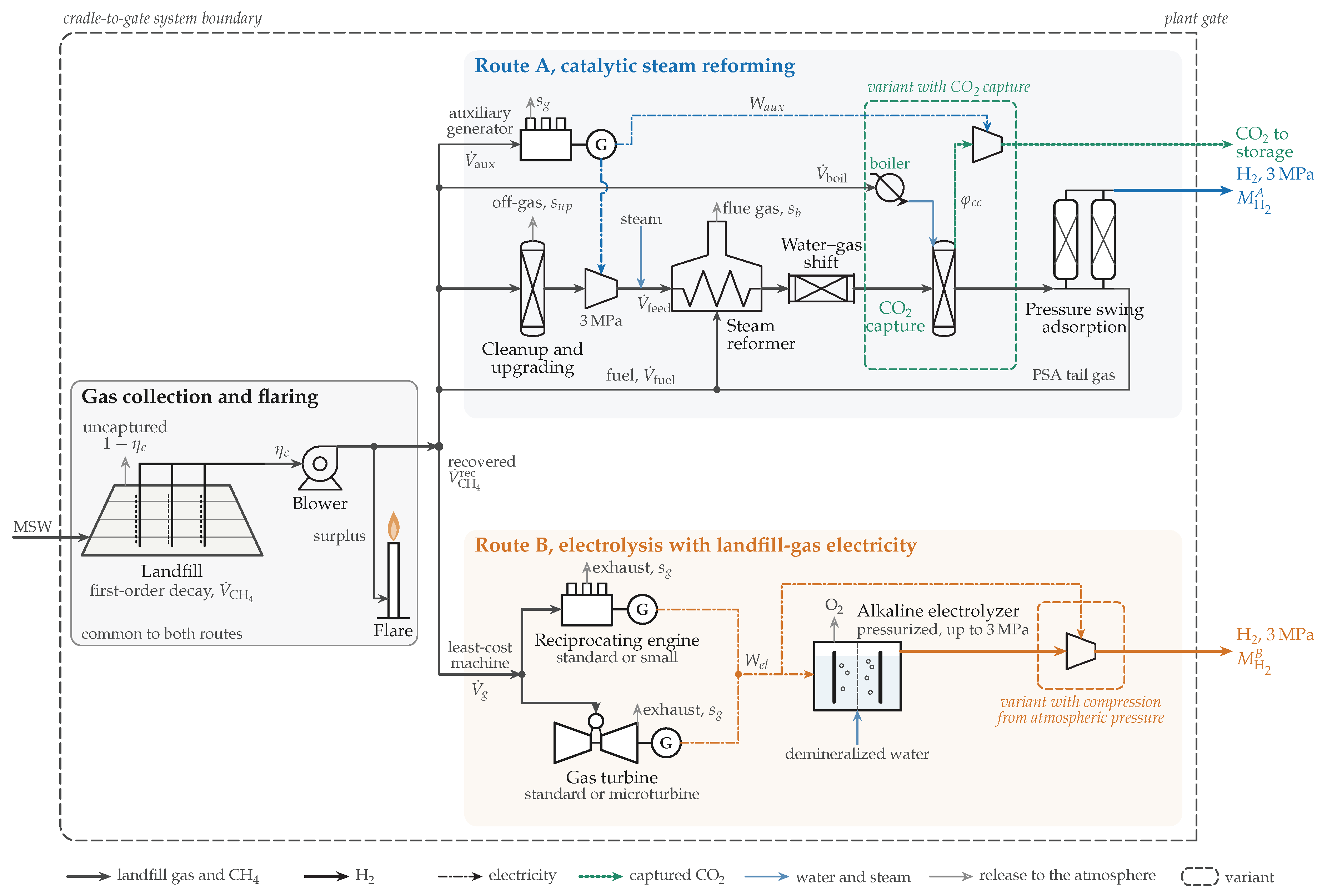
Figure 2.
Cost-capacity relation for reformer islands. Source: own elaboration with data from: [60,61,62,63,64,66,67,68,71,72,73,74,75,76,77,81].
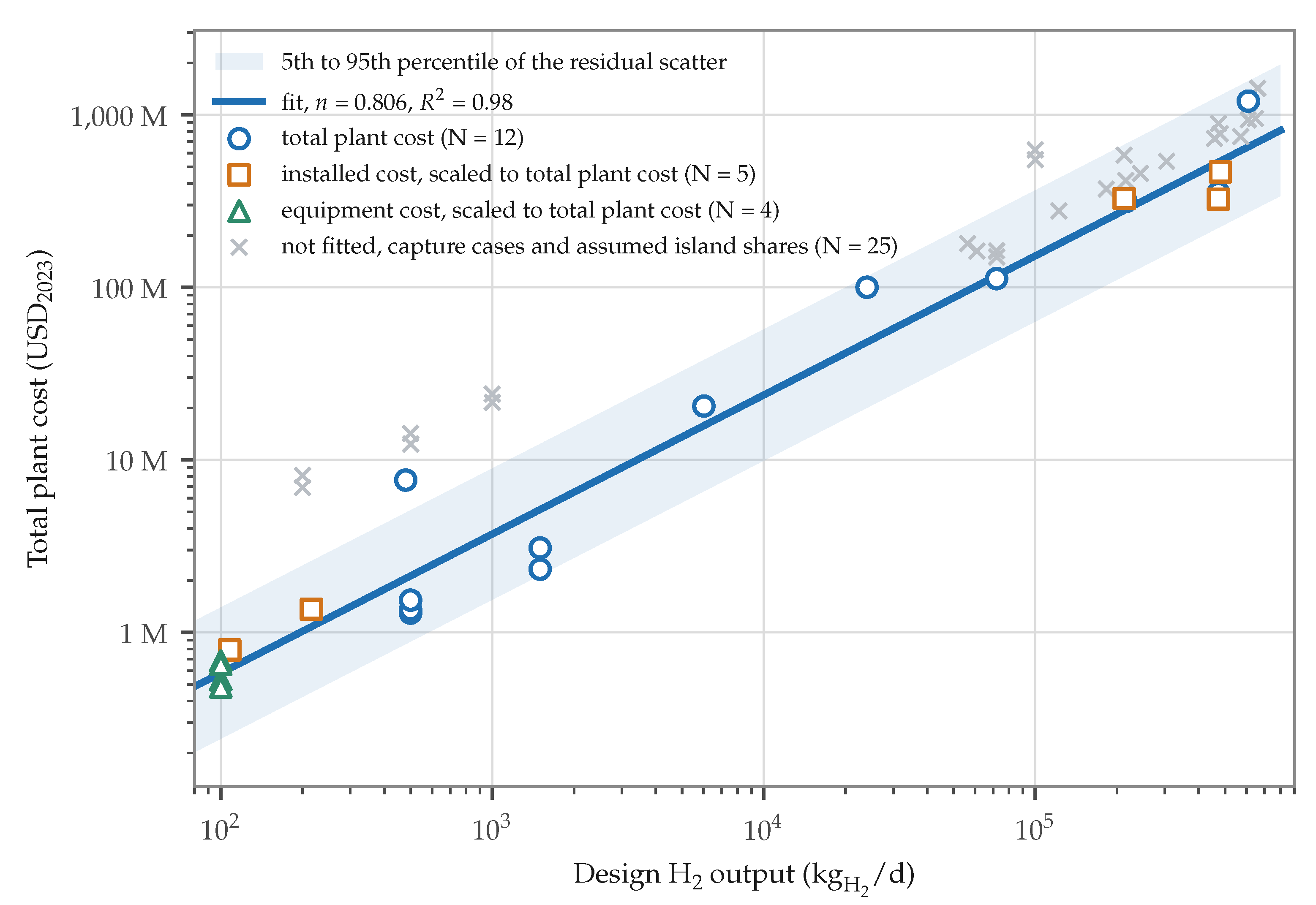
Figure 3.
Technical potential of Route A by site (a) and its concentration (b).
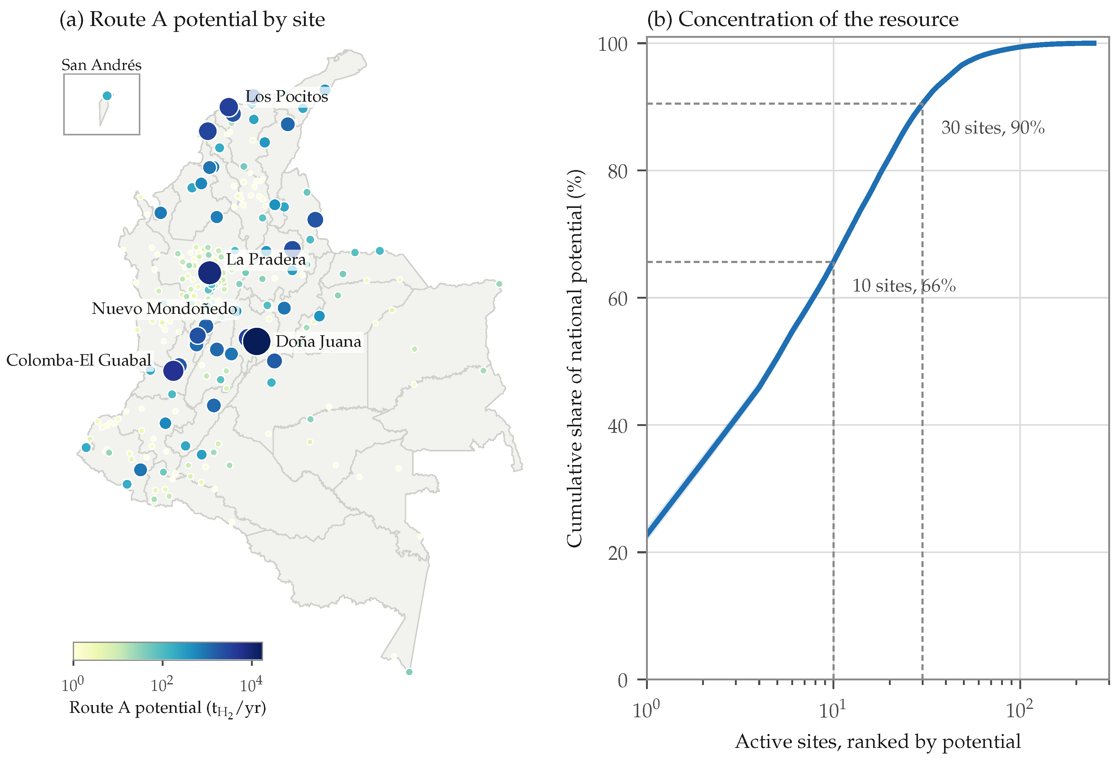
Figure 4.
Licensed life of the active sites (a) and Route A potential by licensed-life group (b).
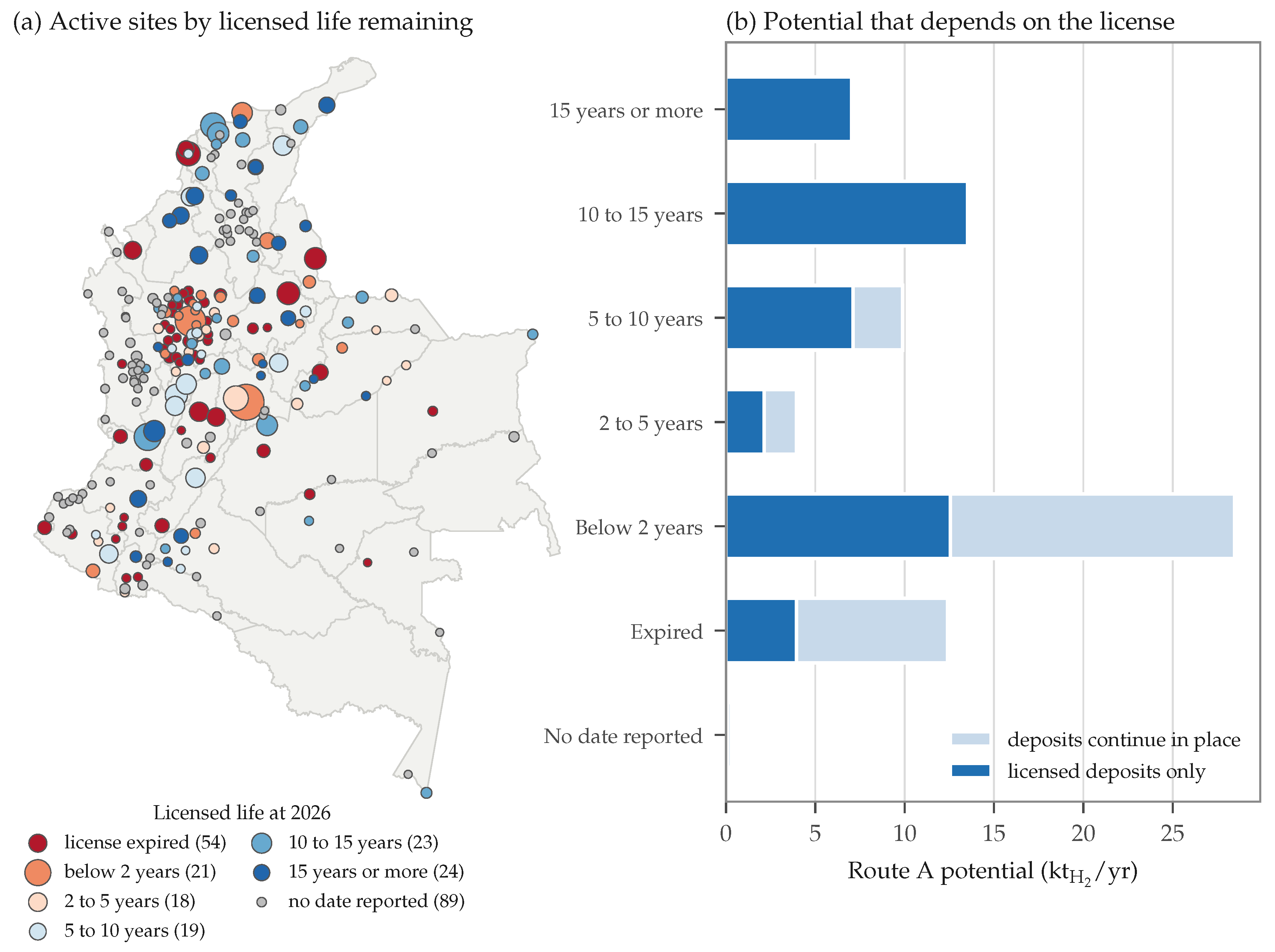
Figure 5.
Supply-cost curves of the three configurations.
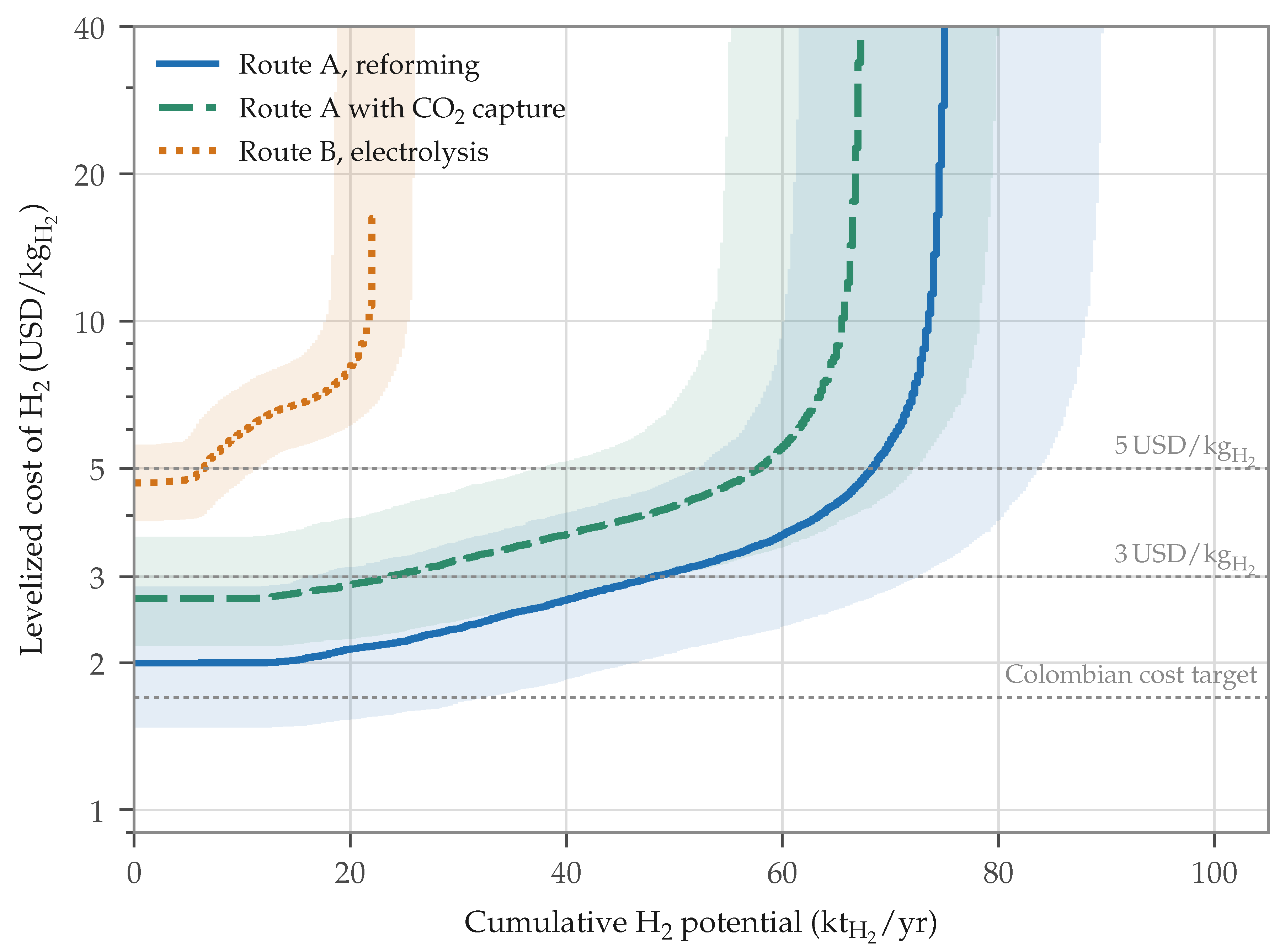
Figure 6.
LCOH and CI by site and configuration.
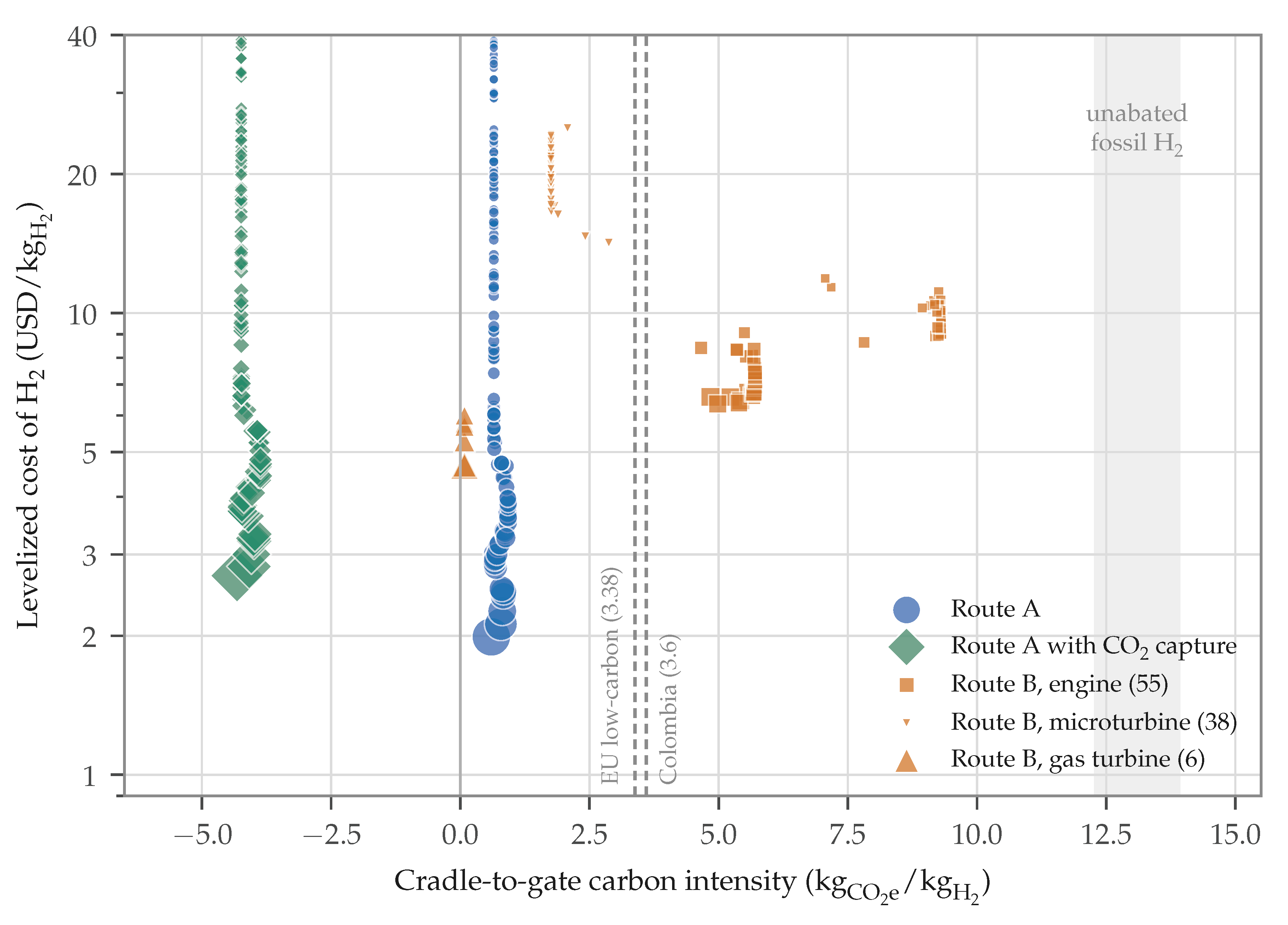
Figure 7.
H2 potential relative to the national agenda (a) and fraction of the potential below LCOH thresholds (b).
Figure 7.
H2 potential relative to the national agenda (a) and fraction of the potential below LCOH thresholds (b).
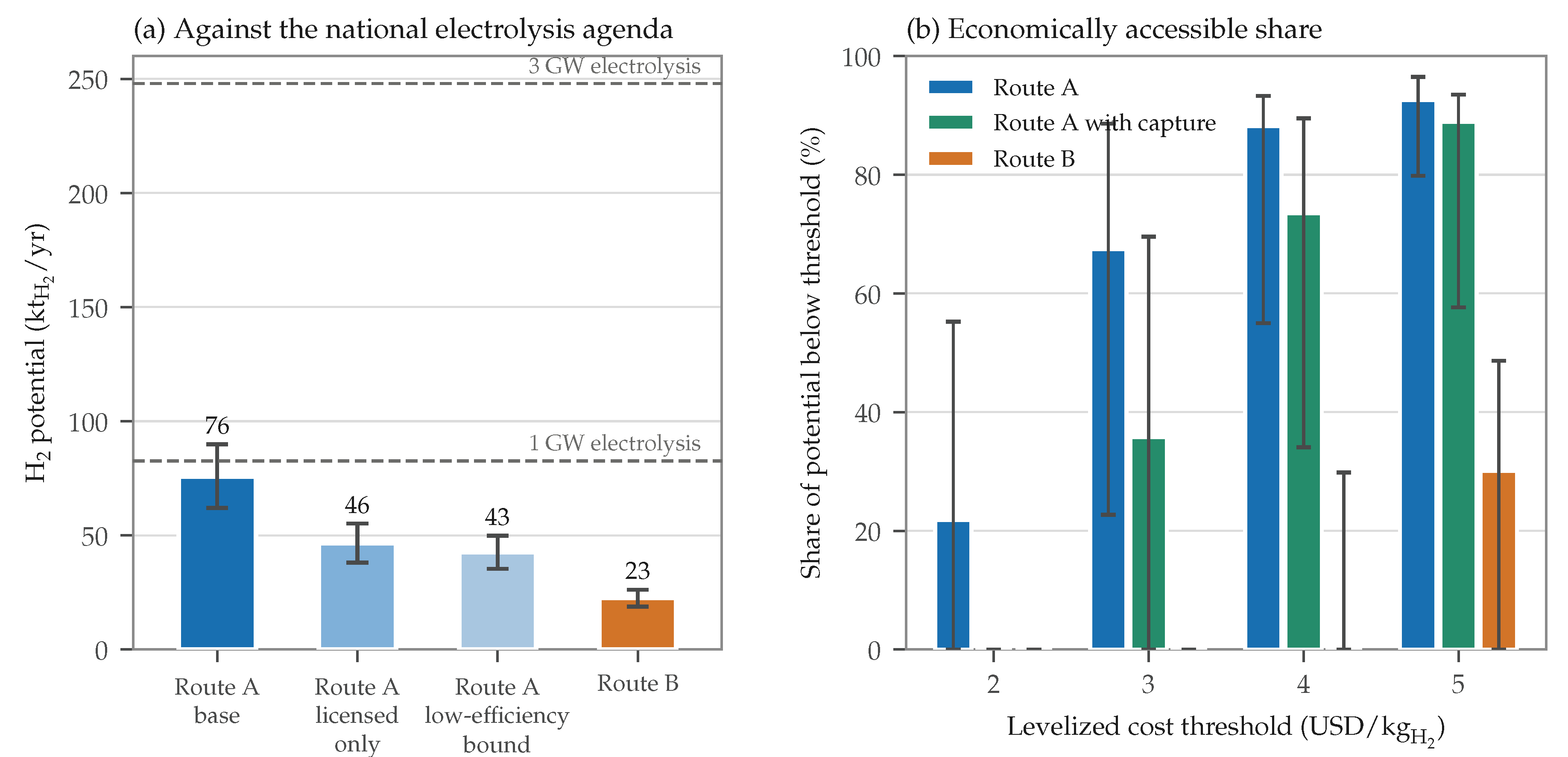
Table 1.
Input datasets and their role in the model. Source: own elaboration with data from: [23,156,159,216,217,218,219,220,221,234,235,236,237].
| Dataset | Role in the Model | Resolution | Period |
|---|---|---|---|
| Disposal registry [23,156] | Mass delivered by each municipality to each site, site class and licensed end of life | Municipality, site | 2010–2024 |
| MSW composition, measured (Table S3) | Biodegradable fractions of the municipalities with a characterization in their PGIRS | Municipality | Latest PGIRS |
| MSW composition, departmental [159] | Fallback profile where no PGIRS reports a characterization | Department | 2018 |
| Population projections of DANE [234] | Per-capita disposal and extension of the deposit series | Municipality | 2005–2042 |
| Climate normals of IDEAM [235] | Precipitation zone of each site | Station | 1991–2020 |
| Inspection reports and project documents [216,217,218,219,221] | Opening years and already existing LFG collection | Site | 2009–2023 |
| Metered LFG record [220] | Validation of the generation model at the largest site | Site | 2021–2025 |
| Published cost estimates for reformer plants | Cost-capacity relation of the reformer (Table S1) | Plant | 2003–2025 |
| Electricity contracts in the wholesale market [237] | Opportunity value of the electricity generated with LFG | National | 2010–2026 |
| Municipal boundaries [236] | Representative point of each site and maps | Municipality | Static |
Table 2.
MSW decay categories and their decay parameters. Source: own elaboration with data from: [125].
Table 2.
MSW decay categories and their decay parameters. Source: own elaboration with data from: [125].
| Decay Category | Composition Fractions Assigned | ( by Precipitation Zone | |||||
|---|---|---|---|---|---|---|---|
| Z1 | Z2 | Z3 | Z4 | Z5 | |||
| 1. Very fast | Food and organics, plus 20 of the sanitary waste | 70 | 0.400 | 0.340 | 0.260 | 0.180 | 0.100 |
| 2. Moderately fast | Garden and pruning | 113 | 0.170 | 0.150 | 0.120 | 0.090 | 0.050 |
| 3. Moderately slow | Paper and cardboard, textiles and 80 of the sanitary waste | 186 | 0.070 | 0.060 | 0.048 | 0.036 | 0.020 |
| 4. Slow | Wood, leather, rubber and bones | 200 | 0.035 | 0.030 | 0.024 | 0.018 | 0.010 |
in Zones Z1 to Z5 receive more than 2000, 1500–1999, 1000–1499, 500–999 and less than 500/.
Table 3.
MSW Composition by Site
| Parameter | Symbol | Value (Range) | Unit |
|---|---|---|---|
| Volume fraction of CH4 in the LFG | 0.50 (0.45–0.60) | ||
| 37.7 | |||
| 33.93 | |||
| 119.96 | |||
| 0.678 | |||
| 2.744 | |||
| 27.0 (100-year) |
Table 4.
Assignment of the national MSW categories to the decay categories. Source: own elaboration with data from: [157,159].
| No. | Reported Category | National Share (%) | Decay Category | Note |
|---|---|---|---|---|
| 1 | Food, pruning and other organics | 61.1 | 1 and 2 | 86 to category 1 and 14 to category 2 |
| 2 | Paper and cardboard | 8.4 | 3 | — |
| 3 | Wood | 2.4 | 4 | — |
| 4 | Rubber, leather, bone and straw | 0.8 | 4 | — |
| 5 | Textiles | 3.1 | 3 | — |
| 6 | Metals | 1.1 | Inert | — |
| 7 | Construction and demolition | 1.5 | Inert | — |
| 8 | Glass and ceramics | 2.2 | Inert | — |
| 9 | Plastics | 11.6 | Inert | — |
| 10 | Sanitary waste and other inerts | 7.8 | 1, 3 and inert | 70.5 sanitary waste, split as in Table 2, and the rest inert |
Table 5.
Coverage of the composition hierarchy. Source: own elaboration with data from: [23,159,160,161,162,163,164,165,166,167,168,169,170,171,172,173,174,175,176,177,178,179,180,181,182,183,184,185,186,187,188,189,190,191,192,193,194,195,196,197,198,199,200,201,202,203,204,205,206,207,208,209,210,211,212,213,214,215].
| Level | Municipalities | Share of Disposed Mass (%) | Range of |
|---|---|---|---|
| Measured characterization | 56 | 64.0 | 56.6–113.0 |
| Departmental average | 1048 | 36.0 | 72.6–96.5 |
| Active sites, weighted by the mass of each year | 248 sites | 100.0 | 71.8–101.6 |
in The shares refer to the mass received by the active sites from 2010 to 2024.
Table 6.
Values of and the by site type. Source: own elaboration with data from: [23,125,133,137,139,156].
| Site Class | Records (%) | Mass (%) | MCF | Range of | Basis | |
|---|---|---|---|---|---|---|
| Sanitary landfill | 85.3 | 95.4 | 1.0 | 0.60 | 0.41–0.71 | Engineered cell, field efficiency according to the cover stage |
| Open dump | 8.8 | 2.0 | 0.8 | 0.05 | 0.00–0.20 | No engineered collection, passive venting |
| Transitional cell | 1.8 | 0.8 | 0.8 | 0.35 | 0.20–0.50 | Partial containment, limited extraction |
| Integral plant | 1.6 | 0.3 | 0.8 | 0.35 | 0.20–0.50 | Cell for rejects after separation |
| Contingency cell | 1.3 | 1.4 | 0.8 | 0.30 | 0.15–0.45 | Temporary cell, no permanent system |
| Burial | 0.5 | 0.1 | 0.4 | 0.00 | 0.00–0.05 | Shallow uncontrolled burial |
| Water body | 0.3 | 0.0 | 0.0 | 0.00 | — | Excluded, no anaerobic cell forms |
| Treatment plant | 0.3 | 0.1 | 0.0 | 0.00 | — | Excluded, MSW diverted from disposal |
| Open burning | 0.1 | 0.0 | 0.0 | 0.00 | — | Excluded, aerobic combustion |
Records and mass are expressed as shares of the 2010–2024 registry.
Table 7.
Evaluated LFGtE technologies. Source: own elaboration with data from: [11].
Table 7.
Evaluated LFGtE technologies. Source: own elaboration with data from: [11].
| Technology | Abbr. | Recommended Size | HR | CF | |
|---|---|---|---|---|---|
| LFG collection and flaring | C&F | Matched to the collected flow | — | — | — |
| Standard reciprocating engine | ENG | ≥ 800 | 11.9 | 0.93 | 0.93 |
| Small reciprocating engine | SENG | 1001000 | 19.2 | 0.92 | 0.93 |
| Standard gas turbine | TUR | > 3 | 13.7 | 0.88 | 0.93 |
| Microturbine | MTUR | 30750 | 14.8 | 0.83 | 0.93 |
| LFG cleanup and upgrading | RNG | 170010200LFG/ | — | — | 0.93 |
HR in based on the HHV.
Table 8.
H2 conversion parameters of the two routes. Source: own elaboration with data from: [10,11,12,38,39,46,49,58,59,60,78,79,80,81,82].
| Parameter | Symbol | Value (Range) | Unit | Source |
|---|---|---|---|---|
| Overall reformer efficiency at 1.5H2/day | 0.60 (0.52–0.72) | — | [60,78,79] | |
| Overall reformer efficiency at 216H2/day | 0.76 (0.72–0.77) | — | [80,81,82] | |
| Conservative bound of the overall efficiency | E | 0.35 | — | [10] |
| Reforming conversion efficiency | 0.75 (0.65–0.88) | — | [10] | |
| Auxiliary electricity | 0.25 (0.15–0.35) | } | ||
| CH4 lost in upgrading | 0.005 (0.001–0.020) | — | [12,38,39] | |
| Electrolyzer SEC | 53 (50–57) | } | ||
| Electrolyzer CF, equal to that of the generator | 0.93 | — | [11] | |
| Water consumption | 12 | } | ||
| Route A yield per unit of island CH4 | 0.170–0.215 | } | ||
| Route A yield per unit of recovered CH4 | 0.144–0.174 | } | ||
| Route B yield per unit of recovered CH4 | 0.034–0.056 | } |
Table 9.
Cost-capacity regression for reformer islands. Source: own elaboration with data from: [60,61,63,64,66,68,71,72,74,75,81].
| Term | Coefficient | Standard Error | Clustered Error | 95% Interval | p |
|---|---|---|---|---|---|
| Constant | 9.560 | 0.406 | 0.560 | 8.702 to 10.417 | <0.001 |
| Scaling exponent n | 0.806 | 0.042 | 0.041 | 0.718 to 0.894 | <0.001 |
| Equipment scope | -1.749 | 0.358 | 0.410 | -2.504 to -0.994 | <0.001 |
| Installed scope | -0.281 | 0.285 | 0.327 | -0.881 to 0.320 | 0.338 |
Dependent variable , in 2023 USD, with 21 observations, of 0.976 and residual standard error of 0.532.
Table 10.
Cost base years and plant cost index values. Source: own elaboration with data from: [84].
Table 10.
Cost base years and plant cost index values. Source: own elaboration with data from: [84].
| Cost Term | Base Year | Index | Escalation to 2023 |
|---|---|---|---|
| MTUR | 2006 | 499.6 | 1.597 |
| SENG; TUR | 2008 | 575.4 | 1.387 |
| C&F; ENG | 2013 | 567.3 | 1.406 |
| CO2 capture and compression | 2018 | 603.1 | 1.323 |
| RNG train | 2019 | 607.5 | 1.313 |
| Reformer island; electrolysis system | 2023 | 797.9 | 1.000 |
Table 11.
Economic parameters of the LCOH calculation. Source: own elaboration with data from: [11,48,50,59,84,86,87,88,108,109,112,113,237].
| Parameter | Symbol | Value (Range) | Unit | Source |
|---|---|---|---|---|
| Discount rate | i | 0.09 (0.06–0.12) | — | [11] |
| Project lifetime | — | 15 | } | |
| MTUR lifetime | — | 10 | } | |
| Electrolyzer stack replacement interval | 9.2 | } | ||
| Availability of the conversion units | — | 0.93 | — | [11] |
| Cost reference year | 2023 | — | [84] | |
| Reformer reference CAPEX at 1500H2/day | 5.15, lognormal | } | ||
| Reformer scaling exponent | 0.806 (0.718–0.894) | — | Table 8 | |
| Electrolyzer reference CAPEX at 1 | — | 1800 (900–2600) | } | |
| Electrolyzer scaling exponent | 0.78 (0.70–0.90) | — | [48,88] | |
| Upgrading exponent below the correlation range | 0.65 (0.50–0.80) | — | This study | |
| LFG purchase price | — | 0 | } | |
| Demineralized water price | 1.50 | } | ||
| CO2 capture and compression | 60 (45–75) | } | ||
| CO2 transport and storage | 40 (20–80) | } | ||
| Electricity opportunity value | 0.088 (0.055–0.095) | } | ||
| Marginal tax rate | — | 0 | — | Public projects |
2023 USD, unless a base year is stated.
Table 12.
Reference values for the cradle-to-gate CI. Source: own elaboration with data from: [13,14,96,97,98,238].
| Reference | Value | Source |
|---|---|---|
| Colombian ceiling for low-emission H2 | 3.6 | [14] |
| EU, 70 saving against 94CO2e/ | 3.38 | [96,97] |
| EU, 65 saving for biomass fuels in transport | 3.95 | [13] |
| Fossil H2 without carbon capture | 12.3–13.9 | [98] |
| Electrolysis with grid electricity in Colombia, counterexample | 11.7 | [238] |
Values in
Table 13.
Input distributions of the Monte Carlo simulation.
| Parameter | Distribution | Support | Rationale |
|---|---|---|---|
| Decay constant | Triangular | Adjacent precipitation zones | Zone assignment is uncertain near the boundaries |
| Potential capacity | Triangular | ±25 | Spread of the published values by category |
| MSW composition | Log-ratio normal | Sums to 100 | The compositional constraint must hold |
| Collection efficiency | Triangular | Table 5 | The same quantile for all sites |
| Baseline efficiency | Triangular | Recorded or assumed range | Measured or inspected destruction |
| CH4 fraction | Triangular | 0.45–0.60 | Varies with cell age and cover |
| Overall reformer efficiency E | Triangular | Table 7 | Scale-dependent plant evidence |
| Reforming conversion | Triangular | 0.65–0.88 | Sets the fuel fraction and the process CO2 |
| Auxiliary electricity | Triangular | 0.15–0.35 | Cleanup and compression demand |
| Upgrading loss | Triangular | 0.001–0.020 | Technology and off-gas treatment |
| Generator slip | Triangular | Section 3.14 | Measured spread by machine type |
| Burner slip | Triangular | 0.00005–0.00025 | Inventory default values for LFG |
| Electrolyzer SEC | Triangular | 50–57 | Depends on technology and load |
| Reformer CAPEX | Lognormal | of 0.532 | Residual scatter of the fitted curve, common to all sites |
| Reformer exponent | Triangular | 0.718–0.894 | Confidence interval of the fit |
| Upgrading exponent | Triangular | 0.50–0.80 | Extension below the correlation range |
| Electrolyzer CAPEX | Triangular | 900–2600 at 1 | Equipment and project scopes differ |
| Electrolyzer exponent | Triangular | 0.70–0.90 | Component exponents differ |
| Capture cost, heat and power | Triangular | Section 3.12 | Stream purity and scale |
| Transport and storage | Triangular | 20–80 | Isolated source or shared hub |
| LFGcost-Web coefficients | Lognormal | ±25 | Regional adaptation of United States data |
| Discount rate i | Triangular | 0.06–0.12 | Public and private financing conditions |
| Electricity value | Triangular | 0.055–0.095 | Range of the contract price series |
Table 14.
Resource and H2 potential of the active sites by site class, 2026 to 2040.
| Site Class | Sites | MSW 2026 | CH4 Generated | CH4 Recovered | H2 Route A | H2 Route B |
|---|---|---|---|---|---|---|
| Sanitary landfill | 158 | 12.21 | 835.3 | 479.3 | 75.17 | 22.50 |
| Contingency cell | 10 | 0.14 | 8.2 | 2.4 | 0.35 | 0.08 |
| Open dump | 73 | 0.20 | 10.7 | 0.8 | 0.12 | 0.01 |
| Transitional cell | 7 | 0.02 | 1.1 | 0.4 | 0.05 | 0.00 |
| All active sites | 248 | 12.58 | 855.3 | 483.0 | 75.69 | 22.60 |
MSW in CH4 in nd H2 in The CH4 columns sum the site medians.
Table 15.
Active sites and Route A potential by licensed life.
| Group | Sites | MSW 2024 | MSW 2010–2024 | H2 Base Case | H2 Licensed Only |
|---|---|---|---|---|---|
| Active, license of 15 years or more | 24 | 1.33 | 10.8 | 7.03 | 7.03 |
| Active, license of 10 to 15 years | 23 | 2.20 | 27.7 | 13.64 | 13.53 |
| Active, license of 5 to 10 years | 19 | 1.62 | 19.8 | 9.88 | 7.11 |
| Active, license of 2 to 5 years | 18 | 0.68 | 8.0 | 3.95 | 2.13 |
| Active, license of less than 2 years | 21 | 3.90 | 53.0 | 28.47 | 12.55 |
| Active, expired license | 54 | 2.23 | 26.7 | 12.41 | 3.95 |
| Active, without a reported license date | 89 | 0.29 | 1.4 | 0.30 | 0.10 |
| All active sites | 248 | 12.25 | 147.4 | 75.69 | 46.49 |
MSW in nd H2 in The values per group are medians of the ensemble of realizations and do not necessarily add up to the total.
Disclaimer/Publisher’s Note: The statements, opinions and data contained in all publications are solely those of the individual author(s) and contributor(s) and not of MDPI and/or the editor(s). MDPI and/or the editor(s) disclaim responsibility for any injury to people or property resulting from any ideas, methods, instructions or products referred to in the content. |
© 2026 by the authors. Licensee MDPI, Basel, Switzerland. This article is an open access article distributed under the terms and conditions of the Creative Commons Attribution (CC BY) license (http://creativecommons.org/licenses/by/4.0/).
Copyright: This open access article is published under a Creative Commons CC BY 4.0 license, which permit the free download, distribution, and reuse, provided that the author and preprint are cited in any reuse.