

Submitted:
13 October 2026
Posted:
14 October 2026
You are already at the latest version
Abstract
The modified Anderson–Björck (modAB) method was first proposed in 2023 by Ganchovski and Traykov for solving nonlinear equations in structural mechanics. It was improved in 2026 with better switching criteria that account for function symmetry and a bisection fallback based on the bracket reduction rate. Although the algorithm performed well in benchmarks, it lacked formal mathematical analysis and proof of convergence. Later analysis by L. Tomov showed some inconsistencies like premature endpoint corrections on the first AB step, and the use of corrected ordinates in the symmetry factor calculation instead of the true residuals. This paper removes the above inconsistencies, provides a proof of global convergence in exact arithmetic, and adds floating-point safeguards for interpolation, method switching and convergence checks, with explicit treatment of infinite and NaN values, underflow, overflow and round-off errors. As a result, the reliability of the algorithm is improved. Performance is also enhanced by an adaptive bisection fallback when AB fails to reduce either the bracket width or the residual, keeping a finite bound on residual reducing steps. Numerical experiments were conducted for an extended set of 100 functions.
Keywords:
nonlinear equations
; root finding
; bracketing methods
; Anderson–Björck method
; regula falsi
; safeguarded interpolation
; adaptive fallback
; global convergence
; floating-point arithmetic
; reproducible numerical experiments
1. Introduction
Finding a zero of a scalar nonlinear function,
is a fundamental task of numerical analysis. Bisection is globally reliable for a continuous function on an interval whose endpoint values on the opposite signs, but it uses only sign information and has linear convergence. False-position methods exploit endpoint ordinates and can be much faster, but the classical version may retain one endpoint for many iterations. The Illinois, Pegasus, and Anderson–Björck modifications were introduced to reduce this endpoint-sticking phenomenon [1,2,3,4]. Other safeguarded approaches include the Brent–Dekker family [5,6], Ridders’ method [7], and the ITP method [8].
The modified Anderson–Björck method was introduced for nonlinear equations arising in structural mechanics [9]. A later implementation combined bisection, an adaptive switching test, corrected false-position steps, and a fallback controller [10]. Subsequent code inspection by L. Tomov revealed some issues that matter both mathematically and computationally. First, the Anderson–Björck correction had been prematurely applied to variables that were later treated as the true values of f at the bracket endpoints. Second, a finite-precision interpolation proposal could participate in a mixed absolute–relative stopping test before being projected back into the bracket. Both issues arise when a quantity used to construct the next iterate is also used, without the necessary checks, to decide that the equation has been solved.
The distinction between a function value and an interpolation ordinate is small in notation but substantial in practice. Rescaling an ordinate changes the line from which the next proposal is obtained without changing the function. Keeping these roles separate lets us first establish that the interval still contains a zero, and then ask whether its width must tend to zero. Bisection supplies one part of the answer. A shrinking reference width, against which each AB phase is tested, supplies the other. A strict width schedule can, however, interrupt an endpoint that is already approaching a zero rapidly and slow down the method. We therefore allow a finite number of exceptions when a new true residual improves on both endpoint residuals by a fixed factor. The resulting bound concerns the complete hybrid controller; it is not a new local order for the classical Anderson–Björck iteration, nor a claim of bisection’s minimax evaluation budget.
The finite exception allowance is a significant part of this guarantee. We exhibit a continuously differentiable function for which the true residual continues to decrease by more than one half per AB step while the bracket width tends to a positive limit. This complements the quadratic example which shows that residual progress explains why an exception can be useful, whereas the counterexample explains why exceptions must be limited. We also prove a cubic bound for the switching expression, separate its exact-arithmetic meaning from floating-point evaluation, and verify the minimal restoration of the exception cap in a later implementation snapshot.
2. The Corrected Hybrid Method
2.1. Terminology and the Idea of the Proof
We use several standard terms in a very specific sense.
A bracket is a closed interval for which the endpoint values have opposite signs:
For a continuous function, the intermediate value theorem then guarantees at least one zero between a and b. The word residual means simply the function value in the real-arithmetic analysis, or when a floating-point evaluation is meant. It is a vertical error in the equation , not automatically a bound on the horizontal error in x.
An ordinate is the vertical coordinate of a point on a graph. Thus and are the true endpoint ordinates. The Anderson–Björck correction temporarily rescales one ordinate before drawing the next secant. We call the resulting values modified ordinates. They are interpolation data, not new values of the function.
An AB phase is a consecutive run of Anderson–Björck steps. A fallback ends such a phase and returns the method to bisection when the bracket has fallen behind its width schedule and no permitted residual exception remains. A step is called nonexpansive in width when it cannot make the bracket wider.
The proof answers two questions in order. First, can the method ever discard all zeros? The bracket invariant shows that it cannot. Second, can the bracket keep a positive width forever? Bisection halves it outright, while an AB phase is compared with a geometrically decreasing reference width. These two facts force the width to zero. The later quantitative argument merely counts how many iterations may be spent for each guaranteed factor-of-two reduction.
2.2. Assumptions and State Variables
The convergence analysis is carried out in exact real arithmetic under the following assumptions.
Assumption 1.
The function is continuous, , and
Unless the method terminates at an exact zero, all endpoint residuals are nonzero.
At global iteration n, the method stores a bracket
and the true endpoint residuals
During an Anderson–Björck (AB) phase, it also stores modified ordinates
They obey
but their magnitudes may differ from the true residuals. A new AB phase starts with
The distinction between the actual values of the function in (3) and the modified values in (4) is essential. The actual values are used to maintain the interval containing the root, to evaluate the switching criterion, and to assess convergence at termination. The modified values enter only the secant formula for the next approximation.
2.3. Successive Approximations and the Enclosing Interval
The method starts with bisection. A bisection step gives the approximation
An AB step uses the false-position formula with the modified ordinates,
If , the method terminates at an exact zero. Otherwise, we replace by the endpoint whose function value has the same sign as . If two consecutive AB steps replace the same endpoint, the modified ordinate at the retained endpoint is multiplied by a finite positive factor . The usual Anderson–Björck rule takes
where is the endpoint to be replaced. After two consecutive replacements on the same side, the ordinate at equals the actual value of the function there, since that endpoint was introduced at the preceding step. The implementation may therefore use the stored interpolation ordinate in this ratio without changing the Anderson–Björck formula. At the new endpoint, the modified ordinate is set equal to .
2.4. Switching Between Bisection and Anderson–Björck Steps
When a bisection step is evaluated at the midpoint , define the midpoint value of the endpoint chord,
and the symmetry factor
The method may switch from bisection to AB steps when
The global convergence proof does not depend on this particular switching criterion. It depends on the condition for returning to bisection, which we specify below.
Lemma 1
(A cubic bound for the switching expression). Let and be nonzero real endpoint values of opposite signs, and put
For any real midpoint residual , let . Then and, in exact arithmetic,
Proof.
The triangle inequality gives
Since , division by D gives . Moreover,
To bound the remaining dimensionless factor, define
Its derivative satisfies
Thus Q is decreasing, and its endpoint values yield . Substitution proves (13). □
The lemma bounds the right-hand side of (11) in exact arithmetic. Section 5.5 gives the corresponding rounding-error analysis: first for the distributed expression when all intermediate results are in the normal range, and then for a scaled evaluation valid throughout the finite binary64 range. Here is dimensionless, whereas has the same scale as the values of the function.
Suppose an AB phase starts immediately after a bisection update and the resulting width is
Within this phase, use local indices: is the interval before AB step t, is the approximation computed at that step, and is the interval length after the endpoint replacement. Thus counts completed AB steps within the phase. Choose , an integer , and a residual factor . Initialize a counter and a width threshold . At step t the threshold used in the comparison is
Before replacing an endpoint, denote the smaller of the two endpoint residual magnitudes by
This minimum is taken over the actual values of the function. After replacing the endpoint, let be the length of the resulting interval and apply the following conditions in order:
- 1.
- If , continue with AB steps and set .
- 2.
- Else, ifcontinue with AB steps and increase c by one.
- 3.
- Else end the AB phase and take a bisection step next. Restore the modified ordinates to the actual endpoint values and discard the record of the endpoint replaced in the preceding AB step.
Whenever the phase continues, halve the threshold for the next step. Allowing an exception on the basis of residual decrease does not restart this sequence of thresholds. Thus the counter records consecutive exceptions to the width condition; it returns to zero when that condition is satisfied or a new AB phase begins.
In the numerical experiments we use
The first two thresholds, and S, are always satisfied because the interval lengths are nonincreasing. The first possible violation of the width condition occurs after the third AB step, when the threshold is . At most three consecutive violations are permitted, and each requires (17). If steps 3, 4 and 5 all require residual exceptions, then the allowance is exhausted before step 6. In that case, the sixth AB step must find an exact zero or satisfy the width condition; else the method returns to bisection. If an intervening step satisfies the width condition, the counter returns to zero and later exceptions remain possible. Thus six is not an upper bound on the number of steps in an AB phase.
The implementation parameter MaxResidualSteps represents the bound M on consecutive exceptions, rather than a bound on the number of steps in an AB phase. A phase can continue for longer if the width condition is subsequently satisfied. The separate parameter MaxIterations bounds the total number of iterations and reaching it may produce MaxIterationsExceeded. Such termination neither forces a bisection step nor implies a bound on the length of the interval. Proposition 3 shows why a bound on the total number of iterations cannot replace the bound on consecutive exceptions.
For the convergence estimates, define
Lemma 5 proves that an active phase satisfies , even when individual width conditions are violated. Thus (18) gives
The same upper bound is obtained for the fixed-delay version by setting and . In that case the first five width conditions hold automatically, and the first comparison with occurs after the sixth AB step. The earlier convention of multiplying the width before the switching bisection by 16 gives the same bound in exact arithmetic, since that bisection halves the interval length. This equivalence in exact arithmetic, however, does not imply bitwise agreement between floating-point implementations.
3. Preservation of the Enclosing Interval
Lemma 2
(Interiority of the AB approximation). Let and . Then
belongs to .
Proof.
Assume without loss of generality that . Then
Thus x is a strict convex combination of a and b and belongs to . The case follows in the same way. □
Lemma 3
Proof.
Multiplication by a positive factor preserves the sign of the retained ordinate. At the new endpoint, the modified ordinate equals the actual value of the function. Since the new interval has endpoint values of opposite signs, the modified ordinates also have opposite signs. □
Proposition 1
(Nested intervals containing a zero). At every nonterminating iteration,
Consequently, every contains at least one zero of f, and the widths
are nonincreasing. A bisection step gives
Proof.
The sign condition holds initially by Assumption 1. The midpoint belongs to the current interval, as does the AB approximation by Lemma 2. Unless this new point is an exact zero, precisely one of the two resulting subintervals has endpoint values of opposite signs. The method selects this subinterval, which contains a zero by continuity and the intermediate value theorem. This proves the nesting property and the monotonicity of the interval lengths. A bisection step gives a subinterval of half the preceding length. □
3.1. Residual Decrease During an Exceptional AB Step
Lemma 4
(Decrease of the smaller endpoint residual). Let before a nonterminating step within the interval, and let be the corresponding minimum after the sign-preserving update. If the new residual satisfies with , then
For k consecutive such steps, the final minimum is less than times its initial value.
Proof.
The retained endpoint has residual magnitude at least . The newly inserted endpoint has residual magnitude below . It therefore becomes the endpoint with the smaller residual magnitude, which proves (24). Repeated substitution proves the last claim. □
The minimum must be taken before replacing the endpoint. After the replacement it would be no greater than , making the strict contraction inequality impossible. In exact arithmetic, replacing f by , , leaves the condition unchanged, since both sides are multiplied by . Residual decrease alone, however, does not give a bound on the error in the root approximation. Near a zero of multiplicity m, the model shows that reducing the residual by a factor reduces the distance to the zero by approximately . The bound on the interval length and the finite number of permitted exceptions are therefore still needed for the geometric convergence estimate. In general, neither AB steps nor bisection steps make the smaller endpoint residual decrease monotonically; the lemma applies only when its contraction hypothesis is satisfied.
3.2. One-Sided Convergence Without Contraction of the Interval
Proposition 2
(A one-sided quadratic AB phase). For the continuously differentiable function
an AB phase starting from with the actual endpoint values as its initial ordinates has a fixed right endpoint. If interpolation is continued without a width fallback, the left-endpoint error converges quadratically to zero, whereas the bracket width tends to one.
Proof.
Write the left endpoint as and the right modified ordinate as . The actual left ordinate is . The next secant approximation is , where
Starting with , the first two errors are and . The second consecutive update of the left endpoint activates the AB correction. Whenever it is applied,
Thus the next trial point remains to the left and, from the error onward,
This positive sequence decreases to zero and . Its first subsequent values are , and . The right endpoint stays at one, so . □
This phase also occurs within the hybrid method. Starting from , the first midpoint is , and the switching inequality is . The method therefore enters the AB phase just as described. Here the left endpoint converges quadratically even though the interval length tends to a positive limit. This is a property of this particular phase only. With only finitely many consecutive exceptions permitted, the method eventually returns to bisection unless it has already satisfied a stopping condition.
3.3. Necessity of a Bound on Consecutive Residual Exceptions
In the preceding example, continued interpolation rapidly improves one endpoint approximation. The next example shows why residual decrease cannot be the only condition for continuing an AB phase: even a uniform reduction by more than one half at every subsequent step need not force the interval length to zero.
Proposition 3
(Residual contraction without width convergence). Consider the usual AB correction, the switching test (11), and the rule with , , but with no bound on the number of residual exceptions. For
the exact-arithmetic process enters an AB phase after its first bisection and never leaves it. The left endpoints converge to the unique zero, while the right endpoint remains 1 and the width tends to 1. From the third AB step onward, the ratio of the new residual magnitude to the smaller preceding endpoint residual magnitude is at most . The function belongs to .
Proof.
The only zero is 0. On the two open half-lines the derivatives are and , respectively. At zero, , and both one-sided derivatives tend to zero. This proves the stated regularity.
Initially and . The first midpoint is , with , and the chord midpoint value is also . Consequently, the left-hand side of (11) is zero and its right-hand side is positive. The method enters AB on .
Let j count AB steps after this entry. Write the left endpoint as and the retained right modified ordinate as , with and . The actual function value at the left endpoint is . If the next trial point remains to the left of the zero, the secant formula gives
There is no retained-ordinate rescaling on the first AB step. Hence
Both approximations lie strictly to the left of zero and are closer to it than the preceding left endpoint.
For two successive updates of that endpoint, the AB multiplier is , which is positive whenever . Rearranging (28) gives
Thus, for while these inequalities hold,
Applying this identity at and then taking the next secant yields
In particular, and .
To prove that all subsequent approximations have the same properties, put . Using (29) in the next secant, we obtain
The last equality divides numerator and denominator by . Define
For and its denominator is positive, and direct differentiation gives
On , , monotonicity therefore gives
Both bounds belong to . Since the required inequalities hold for , induction gives
These inequalities simultaneously prove that the next trial point remains strictly left of zero, that the AB multiplier stays positive, and that the hypotheses are preserved. Thus and the right endpoint is never replaced.
The actual value of the function at the right endpoint is 7 and the left residual magnitude is . Before AB step j the minimum residual magnitude is therefore . For every ,
At the beginning of the phase the width is , so the threshold at AB step j is . The first two interval lengths satisfy the respective bounds 4 and 2. For , however, while . The width condition is therefore violated at every subsequent step, whereas (31) permits a residual exception at each of these steps. Without a bound on their number, the AB phase continues indefinitely and the interval length tends to 1. □
The same example shows that the earlier global estimate cannot be retained after removing the bound on consecutive exceptions. If N counts all bracket updates, including the initial bisection, then and
The approximations themselves still converge to the zero. What fails is convergence of the whole bracket and, consequently, width-based termination at a tolerance below the limiting width. For the mixed tolerance used here, any fixed and finite leave the width test unsatisfied for all sufficiently late steps, since the candidate tends to zero. In particular, the tolerances of the numerical experiment in Section 7.4 cannot terminate this exact-arithmetic process by width. It never encounters an exact zero.
3.4. A Geometric Bound on the Interval Length During an AB Phase
Lemma 5
(Geometric upper bound for an AB phase). Let a phase start with width S, use (15), and permit at most M consecutive width-test exceptions while active. If it is still active after t steps, then
Proof.
If the width condition is satisfied at step t, then , which is stronger than (33). Otherwise, let be the last index at which it was satisfied. Since the phase continues, . If the condition has not yet been satisfied, take and set ; then because . The bracket widths are nonincreasing, so in either case
Whenever the width condition is satisfied, the counter returns to zero and the estimate holds at that index. The same argument therefore applies after any number of such resets. □
The proof depends on the bound on consecutive exceptions, but not on the value of . The residual condition determines when an exception is permitted and the bound on their number gives the estimate for the length of the interval. If an AB step leads to a return to bisection, (33) need not hold after that last AB step. Both this step and the following bisection are included explicitly in the iteration bound derived below.
The result holds for every finite integer , not only for . For fixed B, increasing the number of permitted consecutive exceptions by one doubles the constant . With , the iteration bound below uses . In particular, gives ; every other finite choice also gives an upper bound on the length of the interval. Proposition 3 shows that this estimate cannot be retained if arbitrarily many consecutive exceptions are permitted. It does not single out three as the necessary or optimal finite bound.
4. Global Convergence
The preceding results show that every interval contains a zero. It remains to prove that the interval lengths tend to zero. We first prove convergence and then estimate the number of iterations needed for a given reduction in length. For the latter estimate, we must also account for a final AB phase that has not yet ended.
Throughout this section, denotes the interval length after n completed endpoint replacements, with . We study the iteration without a bound on its length and without a positive stopping tolerance. The process may still terminate at an exact zero. In the implementation, termination at an exact zero or upon satisfying the prescribed width tolerance already gives the required result.
4.1. Convergence of the Enclosing Intervals
Theorem 1
(Global convergence). Under Assumption 1, with the actual function values and modified ordinates kept separate and the adaptive rule of Section 2, the exact-arithmetic iteration, continued without an iteration limit, either terminates at an exact zero or satisfies
In the latter case, the nested brackets shrink to a single point , and that point satisfies .
Proof.
We distinguish two cases.
Case 1: infinitely many bisection steps. Each bisection halves the current interval length, and no intervening AB step increases it. After j bisections the length is therefore at most , which tends to zero.
Case 2: finitely many bisection steps. After the last bisection, all subsequent steps belong to a single AB phase. Indeed, ending that phase would require another bisection, contrary to the choice of the last one.
Let be the width at the start of that phase and let be the width after t AB steps. Because the phase is still active, Lemma 5 gives
The right-hand side tends to zero, and hence so does .
Thus in either case. By Proposition 1, the closed intervals are nonempty, nested, and contain a zero. A standard nested-interval argument now shows that their intersection consists of one point:
To verify that this point is a zero, choose any zero . Both and lie in the same interval, so
Thus . Since and f is continuous, . □
Remark 1
(Scope of the convergence argument). The argument does not assume differentiability, a unique zero, a particular local convergence order, or the specific switching test (11). It uses only intervals whose endpoint values have opposite signs, interpolation points within these intervals, nonincreasing interval lengths, the geometric upper bound during each continuing AB phase, and the bisection step that follows the end of a phase.
4.2. An Upper Bound on the Number of Iterations
To obtain a quantitative convergence estimate, define
The integer d is chosen so that . The additional two iterations in q account for the last AB step of a phase and the bisection step that follows it.
We say that a sequence of iterations gives h halvings if its final interval length, relative to the initial length S, is at most
This terminology describes the reduction in interval length; it does not require the sequence to contain h actual bisection steps.
A completed phase block consists of an AB phase with AB steps, followed by the first bisection after fallback. Its total length is .
Lemma 6
(Guaranteed shrinkage of a completed AB phase). Let a completed phase block start with width S. At its end the width is at most , where
In both cases,
Proof.
We consider the two ranges of t separately.
If , the AB steps do not increase the interval length, and the following bisection halves it. Thus , and
Now suppose that . The phase was still active after step . Lemma 5 therefore gives
where the last inequality uses . The tth AB step cannot increase the width, and the following bisection divides it by two. Hence
The block therefore guarantees halvings. Since and ,
□
Table 1 summarizes the two estimates. For a short AB phase, the following bisection alone gives the required reduction. For a long phase, the geometric bound already implies a stronger reduction before that bisection.
The first n iterations may end within an AB phase or just after its last AB step, before the following bisection. We therefore also need an estimate for this possibly incomplete final part.
Lemma 7
(An incomplete final AB phase). Suppose the first n iterations end either within an AB phase or immediately after its last AB step, before the following bisection. Let S be the interval length at the start of this final AB phase. If the unfinished part has length , then there is an integer such that its final width is at most and
Proof.
Let t be the number of AB steps in the unfinished part.
If the phase is still active and , take . Then . If the phase is still active and , Lemma 5 gives
Thus we may take , and .
It remains to consider a final AB step that has just triggered fallback. If , again take ; then . If , the phase was active after step , so
Now take . Since ,
These cases cover every possible unfinished final part. □
Theorem 2
(A global bound on the interval length). Under the assumptions of Theorem 1, after any n completed bracket updates, unless an exact zero was found earlier,
Proof.
Partition the first n iterations into:
- bisection steps not already included in a completed phase block;
- completed phase blocks from Lemma 6;
- at most one unfinished final part from Lemma 7.
Let H be the sum of the numbers of halvings given by these parts. A single bisection has length 1 and gives one halving. Each completed phase block of length ℓ satisfies , while the incomplete final part satisfies the bound in Lemma 7. Adding these inequalities gives
Because H is an integer, this implies
Indeed, if , then
which is impossible. The accumulated halvings give , and the stated bound follows. □
Corollary 1
(The adaptive method with and ). For the adaptive method in exact arithmetic with , and ,
and therefore
Figure 1 shows the common geometric upper bound used in the proof, which is also the fixed-delay threshold. In the fixed-delay version, the first five width conditions hold automatically. In the adaptive version, only the first two hold automatically; up to three consecutive exceptions are then permitted when the residual decrease is sufficient.
Corollary 2
(Finite termination for an absolute width tolerance). Let , and suppose the method stops as soon as . Define
Unless an exact zero is found earlier, . Thus the method terminates after at most
bracket updates. For , one may take .
Proof.
If an exact zero is found earlier, the conclusion is immediate. Otherwise, by the definition of K, . Applying Theorem 2 at gives
□
4.3. An Error Bound at Termination
Let
be the set of all zeros in the initial bracket. If the algorithm returns a point after a width test , then
Here means the distance from to the nearest zero in Z. The estimate is immediate: the current bracket contains at least one zero z, and both and z lie in an interval of width at most .
Using the whole zero set rather than a preselected zero is standard in variational analysis [11,12]. It is also natural for periodic functions or for a bracket containing several zeros.
A small residual alone is not a scale-independent error bound. If, however, the bracket contains a unique zero , f is differentiable, and
throughout the bracket, the mean value theorem gives
5. Implementation and Reliable Stopping
In the C# implementation, the endpoint coordinates are stored in p1.X and p2.X. The fields y1 and y2 retain the actual function values and , whereas p1.Y and p2.Y hold the modified ordinates u and v. This separation is the main correction. A change to u or v changes the next interpolation point; it must not change which signs define the bracket.
5.1. Correspondence Between the Method and Its Implementation
The two implementation variants number their corrections separately. Table 2 brings together the six changes in ModAB3C and the two additional structural changes in ModAB3. The third numbered comment in the simplified method concerns the common secant safeguard and is included in row 2. These eight changes describe the relation to the earlier implementation; they are not eight separate modifications of the convergence theorem. Row 6 concerns the fixed-delay version. The adaptive residual rule replaces that delay, while retaining the separation of actual and modified ordinates and the same sign-preserving interval update.
In row 8 only the comment was wrong: the endpoint-update branches were already consistent with the stated convention. The value zero means that no AB step precedes the current step in that phase. Correcting this description doesn’t change the iteration sequence or the proof. Similarly, centralizing the secant safeguards removes a local Clamp call and duplicate non-finite checks without introducing a new interpolation formula.
Further corrections address overflow when computing the interval length, rounding of the midpoint outside an interval with subnormal endpoints, and a final width check after the iteration limit. These corrections, described below, were proposed in the subsequent review and are separate from the eight changes in the table.
5.2. The Iteration in Finite Precision
The following procedure specifies the adaptive method together with the additional finite-precision safeguards proposed in the earlier review. The switching test always uses the endpoints before the current bisection update. Its decision takes effect after that update.
- 1.
- Order the finite endpoints , evaluate their actual function values, and reject NaN or equal nonzero endpoint signs. Return an endpoint if its actual function value is a machine zero. Set , select bisection, and clear the record of the last endpoint moved in an AB phase. The tolerances must be finite and nonnegative.
- 2.
- Construct the midpoint in bisection mode or the weighted secant point in AB mode, using the safeguards below. Test the current width at this safeguarded point x. If the width test passes, return x. Otherwise evaluate the actual function value there, reusing or if rounding has made x coincide with an endpoint. A machine zero terminates the iteration; NaN gives an invalid-result status.
- 3.
- In bisection mode, evaluate (11) from the actual endpoint values before replacement and the new midpoint residual. Non-finite residuals disable switching. This decision does not yet change the mode used for the current update.
- 4.
- Before replacing an endpoint in an AB step, save from the actual pre-update endpoint values. For either kind of step, identify the endpoint whose actual function value has the same nonzero sign as the new residual. In an AB step, if that endpoint was also replaced on the preceding AB step, multiply the retained modified ordinate by the factor in Section 2; replace a nonpositive or non-finite computed factor by . In both bisection and AB steps, replace the identified endpoint and assign the new value of the function both as its actual value and as its modified ordinate. In an AB phase, record which endpoint was replaced. The actual function value at the retained endpoint remains unchanged.
- 5.
- After an AB update, first test . If it passes, reset the exception counter. Otherwise allow continuation only if and the counter is below M, incrementing the counter in this case. If neither condition permits continuation, select bisection, restore and clear the side record. Halve the threshold only for a continuing phase. After a switching bisection, start a phase with threshold , counter zero and an empty side record.
- 6.
- Repeat up to the chosen update limit. After the last allowed update, test the width once more at the safeguarded midpoint. If this test also fails, return a maximum-iterations status rather than a successful root.
Sign comparisons and termination at a computed zero use only the actual function evaluations. Comparing signs directly avoids forming a residual product that might overflow or underflow. The function is evaluated through a wrapper local to each invocation, but the C# property EvaluationCount remains a shared counter. The local callback prevents nested or parallel calls from replacing the function being evaluated; it does not make that shared count a reliable per-call result under concurrency. The revised benchmark therefore counts evaluations in its own local wrapper. An endpoint residual reused from storage is not a new function evaluation.
5.3. Floating-Point Safeguards
Let be the largest finite binary64 number. For nonzero finite modified ordinates set and and evaluate the secant as
If , first divide both magnitudes by their maximum. If the magnitudes or denominator are unusable, or the final weighted sum is non-finite, use the midpoint instead. Compute that midpoint as , then project the result onto . The secant result is projected in the same way. Even the midpoint needs this last check: separately halving two equal smallest positive subnormal endpoints rounds both halves to zero.
The switching factor can be evaluated from the magnitudes of the actual endpoint values as
Normalize these magnitudes by their maximum when it is at least . Form the chord midpoint as . When either magnitude in (11) is at least , divide the midpoint residual and chord value by their common maximum before comparing the two sides. The comparison remains strict.
After an AB multiplication, a modified ordinate that underflows to zero is replaced by the smallest positive subnormal number with its previous sign; an infinite product is replaced by the corresponding signed value . These replacements affect only the interpolation ordinates. They do not correct errors in function evaluation or establish the sign of the underlying real-valued function.
The pinned ModABCorr snapshot used for the controlled numerical comparison retains the direct midpoint , the direct width comparison, and the update-limit return without the additional final-width check. The projection of a subnormal midpoint and the overflow-aware width comparison described here are further safeguards from the earlier review, not changes silently inserted into that experiment. The reported ordinary-scale cases do not validate these extreme-value paths.
The two earlier stored variants differ when an AB step returns an infinite true residual. The commented ModAB3C skips the AB rescaling for that step, updates the bracket using signs of the actual function values, restores the modified ordinates, and forces the next step to be bisection. The simplified ModAB3 may retain that value while its AB rule remains active; an unusable secant then produces a midpoint through the shared helper. The two variants therefore need not give bitwise identical results in these exceptional cases. Infinite actual function values lie outside Assumption 1, so this difference does not change the exact-arithmetic convergence result.
5.4. Evaluation of the Switching Expression
A later implementation snapshot, commit 51a6d1b [13], evaluates the right-hand side of (11) in distributed form,
and retains a finite-value check on before attempting the switch. Opposite signs prevent overflow in for finite inputs, but not in . If the latter is non-finite, the implementation remains in bisection mode. Lemma 1 bounds the exact distributed expression by . The rounding-error estimates in Section 5.5 distinguish the accuracy of this distributed evaluation from a uniform guarantee for a scaled variant.
In floating-point arithmetic, the equivalent expression can behave differently: the sum in parentheses may overflow before multiplication by k reduces its magnitude. With and
the C# check gives approximately for the distributed expression and Infinity for the grouped one. These results are recorded with the separate snapshot experiment in Section 7.4.
The same distinction between exact algebra and evaluation order applies to a weighted secant. A convex-combination formula is bounded in exact arithmetic, but its independently rounded weights need not sum to exactly one. In the later snapshot, projection onto the finite bracket also handles an infinite weighted sum. For example, magnitudes , and endpoints , give an infinite raw weighted sum in the C# check, and projection returns b. This calculation illustrates the role of projection in that particular case but it does not establish correctness for all exceptional inputs.
The arithmetic simplifications concern the evaluation of each step, whereas the bound on consecutive exceptions concerns convergence of the intervals. The minimal correction examined below keeps the simplified arithmetic and restores only that bound and the strict residual inequality. The additional midpoint and interval-width safeguards are separate.
5.5. Rounding Errors in the Switching Criterion
The cubic estimate concerns the exact value of the switching expression. To study its evaluation, we regard the supplied binary64 numbers as exact input data, with and all three values finite. Here denotes the computed midpoint residual. Errors already present in these function evaluations are not included in the following bounds. Thus the comparison to be reproduced is
where are defined by (12).
We assume binary64 arithmetic with rounding to nearest, ties to even, and gradual underflow. Write fl for a single correctly rounded operation, and put
The indicated order of operations is part of the analysis and intermediate results are rounded to binary64, without reassociation or replacement of separate operations by fused operations. These are the usual rounding assumptions [14,15,16].
5.5.0.1. The unscaled distributed expression.
Consider the evaluation
As in the implementation described above, a non-finite precludes switching.
Proposition 4
(Error bound when the relative rounding model applies). Suppose no operation in (45) overflows, and every nonzero exact intermediate result lies in the normal range. With ,
The subtraction in this bound is an exact subtraction of the two computed numbers. In particular, the comparison agrees with whenever .
Proof.
Under the stated assumptions, division of the rounded sum by two is exact, and
The quotient estimate accounts for the rounded endpoint sum, endpoint difference and division. It follows by bounding the relative factor , where . If , the corresponding quantities are zero and the estimate remains valid.
The subtraction defining and the subsequent square give
Indeed, their relative factor contains the rounding error of the subtraction twice and that of the multiplication once. Since and , both and belong to . Therefore
Also . For the left-hand side,
For the right-hand side, the two rounded products and their rounded sum differ from by at most . Hence
Adding the last two estimates gives
This proves the bound and the assertion about the strict comparison. □
The normal-range assumption matters. For example, let , and . In exact arithmetic,
In (45), however, because the tie rounds to zero. Consequently and : the computed comparison declines a switch that the exact comparison permits. The exact cubic bound therefore does not imply agreement of the two decisions. Nor does Proposition 4, which assumes that overflow has not occurred, prove its absence at the largest input magnitudes.
5.5.0.2. A scaled evaluation valid throughout the finite range.
Both restrictions can be avoided by evaluating the symmetry factor and the two sides with separate scales. Let
These definitions use exact real arithmetic. Since the endpoint values have opposite signs,
The exact normalized difference is
Thus is precisely the original switching condition.
Compute the factor in the following order:
Next compute
The maximum defining s selects an input magnitude and requires no rounding. The endpoint scale in (49) prevents the denominator of the symmetry ratio from vanishing when is much larger than both endpoint magnitudes.
Theorem 3
(A uniform rounding bound for the scaled comparison). For all finite binary64 inputs with , the operations in (49)–(50) produce finite values and have no zero divisor. Under the rounding assumptions stated above, including gradual underflow,
No lower bound on the nonzero input magnitudes is necessary.
Proof.
First observe that rounding any real number in to binary64 introduces absolute error at most . The largest spacing below 2 is ; subnormal spacing is smaller. This absolute bound therefore remains valid when relative error estimates fail near zero.
The computed ratio satisfies . Consequently,
Division of by two is exact: either , or and . Thus all operations defining the factor are finite and their divisors are positive.
To bound its error, note that
Since , replacing by changes by at most . For this fixed , put , and . The rounding bounds give and , while . Hence
Rounding the division adds at most , so . Rounding the next subtraction gives . Both quantities being squared lie in , and therefore
Combining this with the perturbation of proves the first bound.
Each normalized input satisfies and . Rounding preserves the opposite endpoint signs, except that a sufficiently small normalized endpoint may become zero. In either case, and . The endpoint divisions, the addition and the halving therefore give
The last also covers a subnormal halving.
Write and . The subtraction for the left-hand side gives
For the two products on the right-hand side, use , and :
The rounded sum contributes at most another , giving . All these exact intermediate results have magnitude at most 2: the products are bounded by 1 and , respectively, and both sides of the comparison are at most . Thus the absolute rounding bound applies throughout, and no overflow is possible. Finally, rounding their difference contributes at most :
□
Corollary 3
(A sufficient condition for a reliable switching decision). With the scaled evaluation above,
Likewise, implies . If neither inequality holds, retaining bisection avoids an uncertified switch. Every input with is accepted by (52), and every input with is certified as not satisfying the exact switching inequality.
Proof.
Theorem 3 gives in the first case, and the analogous negative bound in the second. Conversely, implies , and similarly for the negative case. □
The number is a dimensionless rounding margin, not a residual tolerance or a stopping tolerance for the root. The constants are conservative bounds, not estimates of typical error. In the subnormal example above, the exact scaled difference is , so the scaled rule accepts the switch. Near equality, however, a strict comparison can change under rounding even when every intermediate result is normal.
A separate Python reference evaluation checked 23,816 input triples against exact rational arithmetic, including extreme exponents, subnormal values, points inside the switching region, and neighboring binary64 numbers at its exact boundary. All five bounds used in the proof, with constants 8, 3, 5, 19 and 25, held in these checks, and every decision certified by the guard agreed with the exact comparison. The same calculation verified (46) on the 22,615 triples satisfying its normal-range assumptions. These are finite checks of the formulas and their reference implementation; the universal claims follow from the proofs above. The concentration of cases near the boundary is deliberate and gives no estimate of how often rounding changes a decision in a practical root-finding problem.
The scaled rule is an additional arithmetic variant and it has not been inserted retrospectively into the C# benchmark results reported in this paper. It preserves the mathematical convergence argument because this argument does not require a particular switching criterion. It does not certify the signs or accuracy of the supplied function values, and it does not extend the exact-arithmetic convergence theorem to arbitrary floating-point function evaluations.
5.6. Machine Zeros and Interval-Width Termination
In binary64 arithmetic, evaluation of the supplied expression defines a computed function . Its exact zero need not be a zero of the real expression f, and a real zero need not evaluate to machine zero. This distinction is standard in floating-point error analysis [14,15,16]. The two stopping conditions are
The candidate must already be finite and inside before its magnitude enters the relative tolerance.
If the directly computed width or tolerance overflows, compare instead
requiring a finite left-hand side. This prevents an erroneous acceptance based on . It is still an ordinary rounded comparison, not an interval-arithmetic certificate.
The geometric conclusion (42) requires the computed endpoint signs to agree with those of a continuous real function, and requires the width comparison not to round an insufficient width into an accepted one. A formally verified implementation would need validated function enclosures and conservative rounding. We do not claim these properties here.
5.7. Changes to the Comparison Methods and Compilation Corrections
We also corrected the implementation of Ridders’ method that we use for comparison. It uses the local callback, recognizes endpoint machine zeros, and rejects NaN both at the midpoint and at the subsequent trial point before either value enters a sign update. To protect the interpolation, let m be the midpoint, divide the three residuals by , and denote the normalized values by . The trial point is
If the scale, radicand or final arithmetic is unusable, or the trial point reaches or leaves an endpoint, the already evaluated midpoint is used instead. The stopping test uses the whole bracket width rather than the distance between successive Ridders points. Known midpoint and endpoint residuals are reused, and the sign update retains an ordered bracket. These comparator changes do not enter the ModAB convergence proof.
In the earlier patch the other solver files were adapted to the new Initialize signature by receiving the local wrapper through out F; those call-site edits did not alter their numerical formulas. The later build repair in ModAB3C removed a stale reference to the local Clamp and made the evaluation explicit as F(x3) before passing the value to Node(double,double). This resolves the obsolete-helper and constructor-interface issues without changing the mathematical update.
6. Formal Verification of Switching and Convergence
Theorem 3 separates the error in evaluating the switching expression from any error already present in the supplied function values. The same distinction is retained in the formal proof. The inputs are three finite binary64 numbers, interpreted as exact real numbers, and the assertion concerns the result of the specified sequence of arithmetic operations. Version 0.4.0 of the formalization covers the scaled switching criterion and its error estimates, the cubic bound, the bracket invariants, the phase and global width bounds, exact-arithmetic convergence, the residual-to-distance estimate, and the two exact AB examples. The formal global convergence proof follows the two cases in Section 4: infinitely many bisections and a final continuing AB phase. The unscaled rounding-error analysis is also formalized under its stated normal-range and no-overflow assumptions.
The proof has been checked in Lean 4 using the real-number theory of mathlib and the floating-point definitions and theorems of FloatLib [17,18]. Its first task is to establish the local error bounds from a concrete definition of rounding. Its second task is to show that the operations on binary64 representations have exactly the real values described by this rounding map. Both steps are needed: an estimate obtained by propagating assumed local errors would leave open whether those assumptions hold for the implemented operations.
6.1. The Rounding Map and the Two Divisions by Two
For , let be the unique integer satisfying
and put
Here is the nearest integer to t, with the even integer chosen when the two distances are equal. The lower bound on makes the smallest spacing equal to . It therefore includes subnormal numbers and rounding to zero without imposing a relative error estimate near zero.
The map in (54) has no upper exponent bound. For a value to be a finite binary64 number, it must also satisfy
This additional condition is checked when the real-valued map is related to the finite format. It is not inferred merely from the precision of the significand.
Lemma 8
(Absolute rounding error on the required range). The map rn is nondecreasing and fixes every number representable in its binary grid. Moreover,
Consequently, every rounded value in this statement is finite in binary64.
Proof.
Monotonicity and preservation of representable values are established for the rounding map in the underlying formal theory. To obtain the error bound needed here, suppose first that . Then and hence . Since N changes its argument by at most ,
The remaining values 0, 2 and are representable and are unchanged by rounding. Monotonicity, applied between the fixed points and 2, gives the second inequality in (56). Finally, , so the finite-range condition is satisfied. Each of these steps is checked in the Lean proof; the subnormal range is covered by the same absolute estimate. □
There are two divisions by two in (49)–(50), and their treatment is different. The division of by two is exact. The division used to form may round, since its numerator can be as small as a subnormal number. For example, . The formal evaluation retains a rounding operation at both places and proves that the first one can be removed.
Lemma 9
(Exact halving in the symmetry factor). If , and , then
Proof.
Monotonicity gives . If , then and the assertion follows. Otherwise, the spacing immediately below 1 is , so
More explicitly, every representable is an integer multiple of . The strict inequality therefore gives . For the same upper bound is immediate. This proves that there is no representable number strictly between and 1.
Since is itself representable, monotonicity now gives . Also . Dividing such a representable number by two lowers its exponent by one and preserves its significand; the result is at least and remains within the normal range. It is therefore representable and fixed by rounding. The formal proof establishes both the spacing assertion and preservation of representability under this exponent change. □
6.2. The Finite-Format Statement
Let denote the set of finite binary64 representations and let assign to each representation its exact real value. The two representations of zero have the same value under . Arithmetic on representations is defined with IEEE rounding to nearest, ties to even, including gradual underflow.
For finite operands and an arithmetic operation ∘, the formal library supplies the relation between the executable operation and its exact real result. In the range used here, this gives
where division additionally requires . The result is proved finite as part of the assertion, so is defined on its left-hand side. This is used separately for addition, subtraction, multiplication and division. Absolute value and the selection of a minimum or maximum preserve the corresponding real values exactly.
Write for the binary64 representation obtained by evaluating the scaled difference in the stated order, including the final subtraction. Write for the real-valued expression obtained by placing rn at the same arithmetic operations. In particular, it initially contains ; its simplification uses Lemma 9.
Theorem 4
(Verified correspondence and switching decision). Let , put , and suppose . Define as in (44)–(48). Every intermediate arithmetic result in the evaluation of is finite, and every divisor is positive. Furthermore,
The executable comparisons with the binary64 representations of and consequently satisfy
They select the respective branches whenever or .
Proof.
The hypothesis implies that the endpoint magnitudes and their maximum are positive. It follows that , and . The normalized endpoint values have opposite signs. Their rounded values retain the weak sign inequalities even if one of them becomes zero, and hence .
Monotonicity of rn gives the intervals for the computed factor stated in the proof of Theorem 3, as well as . The exact results to which rounding is applied all belong to . The endpoint maximum and s are positive, , and the remaining divisor is 2. These facts are established before using (58).
Apply that relation successively to the arithmetic subexpressions. For the initial input expressions, equality of real values is the definition of . If equality has already been established for the operands of an operation, its range bound and, where needed, its positive divisor allow (58) to be applied. The new representation is finite and its value agrees with the corresponding rounded real expression. Induction over the expression therefore proves the equality in (59) and finiteness of all intermediate results.
Lemma 8 now supplies each local absolute error bound, and Lemma 9 supplies the exact first halving. The formal real-arithmetic argument then derives the bounds with constants 8, 3, 5, 19 and 25 used in Theorem 3. These bounds are conclusions of the proof, not additional assumptions on the calculation. For example, the change in is bounded algebraically by
The fraction lies in , which proves and supplies the estimate used in the propagation of errors.
Finally, is exactly representable. The comparisons on finite binary64 representations are proved to agree with the strict order of their real values. Applying the error bound gives the implications and the separation conditions, as in Corollary 3. The identity , with , returns the assertion to the original unscaled inequality. □
6.3. Correspondence with the C # Expression and Reproducibility
The accompanying C# implementation of the scaled comparison uses separate addition, subtraction, multiplication and division calls. A small source translator records their arithmetic expressions in Lean, preserving the order and nesting of all 17 operations. Equality with the rounded expression used in the proof is then checked in Lean. In particular, the two products in the right-hand side are rounded separately before their sum is formed. The decimal constant used for the comparison is also checked to equal exactly. The real-value correspondence is sufficient for the switching criterion since the distinction between positive and negative zero cannot change the comparison, and none of the divisors can be zero.
Version 0.4.0 of the development uses Lean 4.34.0 and fixed revisions of mathlib and FloatLib, recorded in the project. Its audit covers 287 lemmas and theorems and checks their transitive axiom dependencies. They use only propositional extensionality, the quotient principle and classical choice from the standard logical foundation [17]. There are no unfinished proofs or additional axioms asserting the correctness of rounding. The source files, fixed dependency revisions, source checksums and verification records are retained with the reproducibility project ModAB.Switching.Lean, which is publicly available in the development repository.
The relation to native execution has a definite scope. The source translator is an inspected component, not a formally verified C# compiler. Lean checks the arithmetic expression that it produces and the executable IEEE model of that expression. Application of the result to a native C# execution additionally requires the compiler, .NET runtime and processor to perform the stated separate binary64 operations, with the rounding and gradual-underflow assumptions of Section 5.5. Their complete implementations are outside the formal proof.
A separate C# verification checks these arithmetic assumptions on the recorded execution environment, .NET 10.0.12 on Linux x64. For the 23,816 input triples described above, all 404,872 arithmetic operations were compared with independent rounding based on exact integer quotients, remainders and parity. A further 14,268 operations exercise boundary cases, including signed zeros, subnormal numbers, normal-range boundaries, ties and overflow. All 419,140 comparisons agree in all 64 bits. These checks support the correspondence for the tested environment; the universal error bound follows from the formal proof.
The verified assertion concerns admissible inputs to the scaled comparison. The C# rejection of invalid inputs is covered by separate tests. Accuracy of the supplied values of the function, the entire floating-point root-finding implementation and the native compiler are not thereby verified. The module Unscaled.lean proves Proposition 4 by propagating errors through the specified sequence of concrete rounding operations under its stated normal-range and no-overflow assumptions. This rounded-real proof does not establish the native C# execution or a separate finite-format correspondence for every operation in the unscaled expression. The scaled comparison remains the separate arithmetic variant specified above, and its verification does not alter the benchmark results for the other implementations.
7. Numerical Experiments and Reproducibility
7.1. Independent Assessment of the Root Approximations
Consider on , with p odd. For , the positive roots are approximately , , and . Yet a false-position trial point can move so little near an endpoint that a step-based test stops far from all three roots. In this case, the small difference between successive approximations is caused by stagnation. The length of the interval remains large because the other endpoint is fixed, so a stopping condition based on that length does not give the same premature termination.
A residual test has a different limitation. Multiplying the equation by a small positive constant leaves its roots unchanged but makes every residual smaller. In floating-point arithmetic the rescaled expression may even underflow to zero away from a mathematical root. For example, a callback evaluating can return zero at , although the horizontal error is . A separate accuracy check based on the same computed zero would inherit this error and would provide no independent information about the distance to the root.
For a supplied reference set within the initial interval, the revised benchmark checks
It rejects non-finite and out-of-interval answers and does not accept as a substitute for this test. The benchmark call passes both requested tolerances explicitly. The proposed IsRoot(x,aTol,rTol) retains an absolute-only default for the optional third argument, so legacy two-argument calls are not silently reinterpreted. It checks finite nonnegative tolerances, finite ordered bounds and candidates, and usable reference roots inside the initial interval. A null or empty reference list cannot validate a result. Non-finite tolerance arithmetic is conservatively rejected; the validator does not evaluate the callback. The reference roots are numerical approximations, not interval enclosures; their accuracy and completeness must therefore be audited before interpreting the resulting classifications as more than reference-based validation. In particular, a benchmark must not reject a different valid root just because its reference list is incomplete.
7.2. Function Evaluation Counts and Classification of Test Problems
The validation and counting rules in this subsection are a further benchmark revision. In the earlier implementation snapshot, Problem.IsRoot could still accept a callback zero after failing its reference-distance test. That fallback is excluded here; the benchmark corrections should not be confused with the eight ModAB changes in Table 2.
Actual callback evaluations are counted by a wrapper local to each benchmark invocation. Solver return status is preserved separately from the reference-based validation status. A failed validation does not overwrite the measured count. The output includes both the raw count and an explicitly labelled penalized cost; the common failure penalty is one larger than the largest observed raw count among the reference-eligible cases in that run. Thus a method that terminates after only two or three evaluations with an inaccurate approximation is not ranked ahead of a successful method. Successful-run summaries and penalized-cost summaries are reported separately.
The broader development benchmark contains 100 cases. Some are deliberately discontinuous or have singular endpoints. Such stress cases can expose implementation behavior, but they are not tests of the convergence theorem under Assumption 1. In particular, the sawtooth cases have jumps through zero that are not roots; a narrow interval straddling such a jump is not a root-containing bracket. These cases are classified separately from continuous sign-changing problems. The controlled comparison below uses the pinned benchmark definitions. Separate explicit examples document the proof mechanism and the machine-zero failures, so these particular checks do not require the whole collection.
7.3. C # Comparison of the Rules for Returning to Bisection
The comparison uses the fixed repository version at commit 9111cdcc6912401eb684a7b771df3a469795d5b8 [19]. We compiled Release with .NET SDK 10.0.401, runtime 10.0.12, on Ubuntu 24.04 x64, using binary64 values, and an update limit of 200. Three variants share the same ModABCorr arithmetic and differ only in the phase-entry threshold and exception cap: fixed delay , early fallback , and adaptive fallback with . Two further runs use the unmodified repository ModAB and ModABCorr, giving 500 solves over the 100 named cases. The instrumented adaptive variant agrees with the unmodified ModABCorr in returned result and callback count on all 100 cases. Function evaluations are counted by a local wrapper; validation does not call that wrapper or the function.
The eight cases without an eligible reference root are excluded from these aggregates. The validator rejects f27, f29 and f75 for all three variants; their 53 measured evaluations in total are retained in the raw 92-case sum, not counted as successful work. The same 89 cases pass for all variants. Removing the discontinuous sawtooth cases f82 and f83 and the singular-endpoint case f100 leaves the 86-case non-stress subtotal. This classification does not replace a full audit of all remaining function and reference definitions. The largest observed raw count on the 92 cases is 55, so the separate failure penalty is 56. It is a scoring convention, not an evaluation count.
Relative to the fixed-delay version, the adaptive rule reduces the total by 17 function evaluations, all on f92–f97, without increasing the count on any case in this comparison. It also avoids the increased counts produced by early return to bisection on f64 and f84. The original repository ModAB is a different baseline: its raw sum is 1626 in this run, equal to the adaptive total, and it takes eight evaluations on f84 rather than nine. Neither the controlled result nor the aggregate supports a universal ranking of the methods. No wall-clock speedup is claimed.
In the pinned test definitions,
Both observed AB phases approach simple roots. At AB steps 3–5, f64 keeps width approximately while its residual falls through , and . The next evaluation is a machine zero. For f84 the corresponding width stays near , while the residual falls through , and . The sixth AB update then replaces the far endpoint, leaving width .
Figure 2.
First AB phases for f64 and f84. Width and residual are normalized by their values at phase entry. The shaded region marks three residual exceptions. The zero at step 6 of f64 is annotated rather than assigned an artificial positive logarithmic value.
Figure 2.
First AB phases for f64 and f84. Width and residual are normalized by their values at phase entry. The shaded region marks three residual exceptions. The zero at step 6 of f64 is annotated rather than assigned an artificial positive logarithmic value.
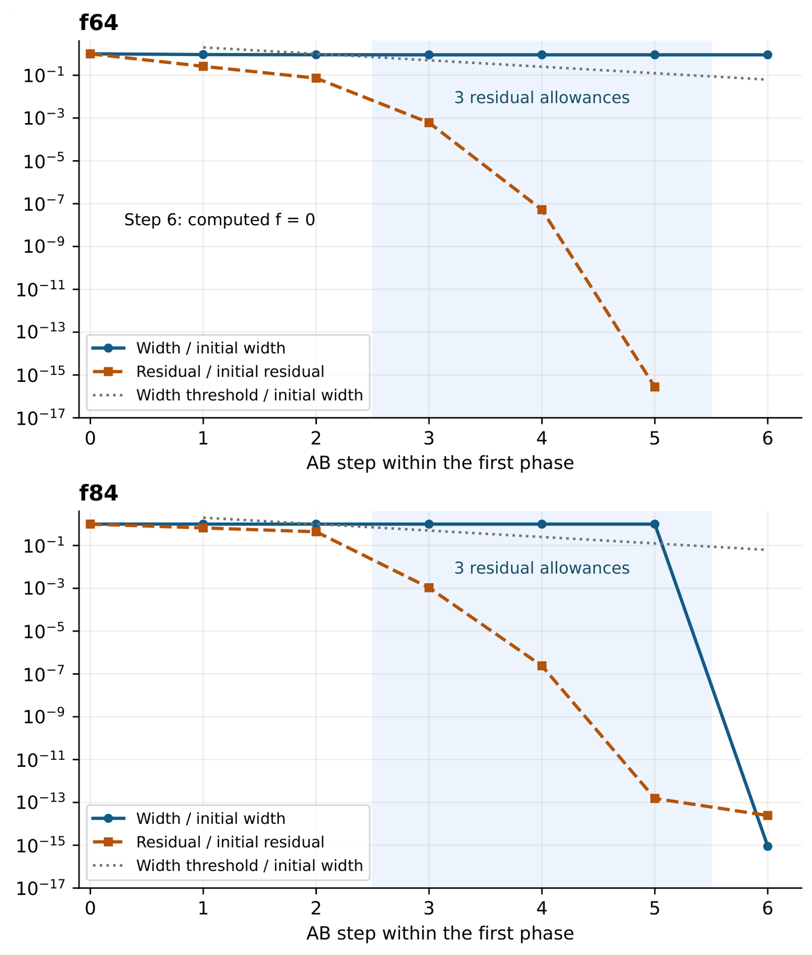
The early fallback on f84 also changes the zero being approached. After its third AB step the bracket is approximately . The following midpoint, , has negative residual, so replacing the left endpoint excludes the nearby zero . The remaining search converges to . The retained interval still contains a zero, as required, but it no longer contains the zero approached by the preceding AB steps. The odd-power cases are different: in their initial flat region the smaller endpoint residual magnitude scarcely decreases, so the adaptive rule returns to bisection without granting exceptions.
7.4. A Numerical Example Requiring the Bound on Residual Exceptions
To examine the effect of the bound on consecutive exceptions in the implementation, we performed a separate experiment on commit 51a6d1b421fa6b5422b974b61c88acb3ae1945bb [13]. This is a later snapshot than the one used in Section 7.3; the two experiments must not be interpreted as using a single source revision. The later SgModAB implementation permits unlimited residual exceptions. The comparison uses that implementation and a minimal patch restoring , resetting the counter at phase entry and after a passing width comparison, and accepting a residual exception only under the strict inequality in (17). Equivalently, a failed width test returns to bisection when the residual is greater than or equal to half the pre-update minimum, or when the allowance has been exhausted. The unpatched comparison uses a strict greater-than rejection and therefore also admits equality; this difference does not affect the counterexample, whose residual ratios are strictly below one half.
The recorded run used .NET SDK 10.0.401, Linux x64, Release configuration, and a limit of 200 iterations. Table 4 gives the results for (27); counts include the two initial endpoint evaluations.
The uncapped implementation exhausts 200 iterations and returns NaN. With the cap, the returned point is approximately and the final width is . The trace contains 75 completed bracket updates followed by a width-based exit on the next loop visit; loop visits and function evaluations are therefore not interchangeable counts. The first forced fallback occurs after the sixth AB step: steps 3, 4 and 5 have consumed the three permitted residual exceptions. This agrees with the rule’s stated order of tests.
We also ran all 100 existing benchmark functions with the unpatched and patched implementations and with tracing copies of each, for 400 solves. For every case the returned value, solver status and actual callback count agree across the four runs. The cap does not trigger fallback on those 100 functions. Both implementations give 1626 evaluations on the 92 reference-eligible cases, of which the same 89 cases pass independent reference validation, totaling 1573 evaluations. The three rounded-zero failures identified in Section 7.5 remain unchanged. The tracing copies also agree with the C# implementations on the added counterexample. The existing benchmark therefore does not establish that the bound on consecutive exceptions can be omitted. These comparisons concern function evaluation counts; they do not measure the additional execution time associated with maintaining the counter.
7.5. Independent Validation of Rounded Zeros
The pinned repository validator ended with return F(x)==0 after its reference-distance test had failed. Removing that fallback changes three classifications in the C# comparison:

Table 5.
Computed zeros rejected by the corrected reference validator. All three rules return these same inaccurate values.
Table 5.
Computed zeros rejected by the corrected reference validator. All three rules return these same inaccurate values.
| Case | Returned point | Mathematical zero | Absolute error |
|---|---|---|---|
| f27 | 1.88916015625 | 1.88889 | |
| f29 | 3.000390625 | 3 | |
| f75 | 0.3333333134651184 |
For f27, the evaluated expression is the expanded form of and loses its small value by cancellation. For f29, rounds to zero before x is close enough to 3. For f75, cancellation occurs in
The known root locations reveal the errors independently of the callback. The revised accuracy check identifies these inaccurate approximations. It leaves the computed values and the solvers’ termination at computed zeros unchanged.
The proposed validator passed 26 C# checks covering these three cases, underflowed callback zeros, exact reference matches, reversed bounds, non-finite candidates, unavailable or unusable references, relative tolerance, invalid tolerances, and overflow. A callback that throws if invoked verifies that validation itself does not evaluate the function. Solver status, external validation status, and raw function counts remain separate fields in the record. The minimal repository patch changes Problem.IsRoot and passes both tolerances at its benchmark call; a separate audit driver supplies the separate evaluation counts and validation results in Table 3.
7.6. Reproduction of the Analytical and Numerical Checks
Exact-rational calculations check the iteration bounds used in the proof. Floating-point examples examine the stopping conditions, the separation of actual and modified ordinates, and the arithmetic safeguards. These checks can be reproduced independently of the complete benchmark collection.
For the first check, normalize and use
The upper bounds on the interval length can be computed recursively. For each number of completed iterations, distinguish intervals obtained by bisection, intervals whose last AB step requires a return to bisection, and intervals within a continuing AB phase. In the last case, record separately for each phase length t the largest possible initial length s. Initially there is only the bisection case, with interval length 1. Halving the larger of the bounds in the first two cases gives the next bisection bound and the initial bound for a possible new AB phase.
After t steps, a continuing AB phase has interval length at most . If it continues for one more step, the corresponding bound is . The last AB step before a return to bisection may retain the preceding bound, but only if that bound is strictly larger than . When several sequences of iterations lead to the same case, retain the largest interval bound, or the largest s for the same phase length. Using exact rational arithmetic, compare the resulting largest bound after each iteration with . All 2700 inequalities held in the earlier check of the reference rule. That calculation concerns the geometric bound on interval length; Lemma 5 establishes its applicability to the adaptive method. These finitely many comparisons supplement the proof of the iteration bound.
For the floating-point tests, use
The unique real root is , and . These are high odd-degree problems with simple roots. For the earlier fixed-delay reference calculation, use binary64 round-to-nearest arithmetic, and hence , , and a limit of 200 updates. Begin with bisection and use the fixed-delay version defined in Section 2. Check the returned point against using (60), rather than accepting a computed zero as an independent accuracy test. Internal reference calculations in Python 3.12.14 on Linux passed this test for all eight cases. The reference root was evaluated as with the platform power function; this is a numerical reference comparison, not a rigorous enclosure of the real root. The C# evaluation counts in Section 7.3 are separate executions; they are not inferred from these Python calculations. No cross-method timing advantage is claimed.
Three arithmetic cases make the safeguards directly testable. With , , , and , the real width is and the tolerance is : the width test must fail even though both unscaled computations overflow. With , the safeguarded midpoint must remain equal to that endpoint. Finally, for at , a machine zero must not pass external root-location validation at tolerance . The internal checks reproduced the unguarded defects and passed with the stated safeguards.
The remaining small checks use with endpoint pairs and , which must return the endpoint root; on with its midpoint evaluation replaced by NaN, which must report invalid input; and on for and . In the last pair, the two returned values differed by at most . These checks passed in the same internal reference calculation.
7.7. Implementation and Supporting Data
The C# implementation is maintained by the second author in the development repository https://github.com/Proektsoft-EOOD/ModAB-Root-Finding. Section 2 and Section 5 specify the method, and Section 7.6 specifies the reported checks. The internal checking scripts are not journal supplementary material. The authors can provide the implementation snapshot and supporting verification records privately to the editor or reviewers on request.
Reproducing the algorithm and matching a particular sequence of binary64 evaluations are different tasks. For the latter, the supplied snapshot must identify the repository commit, runtime and math-library versions, evaluation order, tolerances, update limit, and callback-counting rule. The C# comparison is tied to the immutable commit cited above and to the separately retained validator patch and audit driver. The reference data, raw and validated outputs, build information and source checksums are retained with those records. They can be supplied without adding implementation files to the compact manuscript project.
The separate residual-cap verification package identifies commit 51a6d1b and contains the minimal patch, C# test driver, instrumented copies and raw results, including the counterexample and arithmetic checks. Its reproduction script verifies the commit and an unmodified source tree, builds in a temporary copy and checks agreement of the four benchmark variants. These records are retained separately under Verification/ResidualCap_20260923 and are available from the authors on request; they are not included in the compact manuscript archive or needed to compile the manuscript. They remain separate from the earlier controlled comparison and from the additional extreme-value safeguards.
8. Discussion
An interval can retain endpoint values of opposite signs without its length tending to zero. Interiority of the interpolation point and positivity of the ordinate correction factors preserve the sign condition, but these properties are not sufficient for convergence of the intervals. Ordinary false position already illustrates this difficulty: one endpoint can remain fixed. The geometric bound during each AB phase, together with the bisection that follows its end, ensures the required contraction.
The switching criterion affects the observed convergence rate, but the global proof does not depend on its particular form. Similarly, the Anderson–Björck multiplier influences local convergence, whereas the global argument requires only its positivity and the separation of the actual values of the function from the modified ordinates.
The estimate (40) gives a conservative bound for the hybrid method. It does not describe its local order of convergence. The controlled C# experiment shows an improvement on the specified finite set of problems and identifies errors in the earlier validation procedure, but it does not establish that one method is faster on all admissible functions.
For the adaptive rule, the first two width conditions are satisfied automatically, and at most three consecutive exceptions are then allowed when the residual decreases sufficiently. Lemma 5 therefore gives the same constant as for the fixed-delay version. The last AB step of a phase may violate this bound, but it cannot increase the length of the interval and the following bisection halves that length. Accounting for both steps gives the factor 7 in the global estimate. The residual factor is a dimensionless parameter choice. Its optimality has not been proved, and every fixed gives the same width estimate when B and M are unchanged.
The two exact examples explain the role of the residual condition and the need to limit its use. In the first, one endpoint converges quadratically while the length of the interval tends to a positive limit, so a condition based only on length can interrupt rapid local convergence. In the second, the residual decreases by a fixed factor at every subsequent AB step, yet the interval again fails to shrink to a point. This function satisfies the stated regularity assumptions and involves no extreme magnitudes. The failure therefore occurs in exact arithmetic and is not caused by rounding. In the C# experiment it leads to termination at the iteration limit despite continued residual decrease. A finite M restores the condition needed for convergence of the interval lengths; MaxIterations only bounds the duration of the calculation. The choice retains the existing estimate and the observed evaluation counts on the 100 test problems. Other finite values are allowed by the theory, and this benchmark does not establish which is optimal.
The distinction between actual values of the function and modified ordinates also makes the mathematical method independent of a particular implementation. The proof concerns the interpolation points and the successive enclosing intervals; it does not depend on the names of C# fields or the software framework.
The convergence theorem assumes a continuous real-valued function and exact arithmetic. A supplied computer routine may instead evaluate a discontinuous expression, return NaN, overflow, underflow to zero on an interval, or depend on an internal state. The arithmetic safeguards keep the trial points within the numerical interval and reject NaN, but they cannot ensure that a computed sign agrees with the sign of the underlying real function. Infinite function values also fall outside Assumption 1.
Finite precision also limits the possible contraction of the interval. When its endpoints are adjacent representable binary64 numbers, the computed midpoint may coincide with an endpoint. The exact-arithmetic halving identity then no longer describes the computed step. The implementation therefore uses a positive mixed absolute-relative tolerance and an iteration limit. The theorem establishes convergence of the mathematical iteration; the arithmetic safeguards specify the treatment of exceptional values in its implementation.
9. Conclusions
Our corrections to the modified Anderson–Björck method ensure that the AB rescaling changes only the interpolation ordinates, while the stored actual function values remain unchanged. Keeping these quantities separate allows the actual values of the function to determine the enclosing interval and the modified ordinates to determine the next approximation.
Global convergence follows by considering the number of bisection steps. Infinitely many bisections force the interval length to zero. If there are only finitely many, the final AB phase continues indefinitely, and Lemma 5 bounds its interval length by a geometric sequence tending to zero. Counting the steps in completed phases and in a possibly incomplete final phase gives, for ,
This estimate holds for the iteration in exact arithmetic. Its use as an error bound for computed approximations requires the additional conditions on function evaluation and rounding discussed above.
The residual condition allows interpolation to continue when an endpoint approximation improves rapidly while the interval contracts slowly. The first exact example demonstrates the benefit of this choice. Bounding the number of consecutive exceptions preserves the global estimate for the interval length. The second example proves that removing this bound can prevent the interval length from tending to zero even when the residual decreases by more than one half at every subsequent AB step. Restoring the bound of three consecutive exceptions removes the observed iteration-limit failure without changing the results on the existing 100-case benchmark. The cubic bound for the switching expression justifies a separate simplification of its evaluation; it does not replace the condition needed for contraction of the interval.
Finally, the size of an iteration step, the residual, and the error in the root approximation are distinct quantities. A small step may be caused by stagnation, a small residual by scaling, and a computed zero by rounding. A short interval bounds the distance to a zero only if that interval actually contains one. The independent validation procedure checks the approximation against reference roots, while retaining the original function evaluation counts. This distinction is also necessary in comparisons between methods, where an inaccurate result obtained after few evaluations must not be counted as an efficient solution.
Supplementary Materials
The following supporting information can be downloaded at the website of this paper posted on Preprints.org.
Author Contributions
Conceptualization, L.T. and N.G.; methodology, L.T. and N.G.; software, N.G. and L.T.; validation, N.G. and L.T.; formal analysis, L.T.; investigation, L.T. and N.G.; writing—original draft preparation, L.T.; writing—review and editing, N.G. and L.T. All authors have read and agreed to the published version of the manuscript.
Funding
This research received no external funding.
Institutional Review Board Statement
Not applicable.
Informed Consent Statement
Not applicable.
Data Availability Statement
The test functions, parameters, validation criteria and rule-check procedure are specified in the manuscript. The C# implementation is maintained in the second author’s repository at https://github.com/Proektsoft-EOOD/ModAB-Root-Finding. The Lean formalization is publicly available in the ModAB.Switching.Lean project. Additional supporting verification records and the corresponding implementation snapshot are available from the authors on reasonable request; they can be provided privately to the editor or reviewers during peer review.
Acknowledgments
The authors thank the contributors to the public implementation and benchmark repository. During the preparation of this manuscript, the authors used ChatGPT/Codex for the purposes of manuscript editing and language revision, proof checking, Lean formalization, source-code review and edits, and preparation of test scripts and submission materials. Exact version information for all earlier sessions is not available in the authors’ records. The authors have reviewed and edited the output and take full responsibility for the content of this publication.
Conflicts of Interest
N.G. is affiliated with Proektsoft EOOD, which maintains the software repository discussed in this work. The authors declare no other conflict of interest.
References
- Dowell, M.; Jarratt, P. A modified regula falsi method for computing the root of an equation. BIT Numer. Math. 1971, 11, 168–174. [Google Scholar] [CrossRef]
- Dowell, M.; Jarratt, P. The “Pegasus” method for computing the root of an equation. BIT Numer. Math. 1972, 12, 503–508. [Google Scholar] [CrossRef]
- Anderson, N.; Björck, Å. A new high order method of regula falsi type for computing a root of an equation. BIT Numer. Math. 1973, 13, 253–264. [Google Scholar] [CrossRef]
- King, R.F. An improved Pegasus method for root finding. BIT Numer. Math. 1973, 13, 423–427. [Google Scholar] [CrossRef]
- Brent, R.P. An algorithm with guaranteed convergence for finding a zero of a function. Comput. J. 1971, 14, 422–425. [Google Scholar] [CrossRef]
- Bus, J.C.P.; Dekker, T.J. Two efficient algorithms with guaranteed convergence for finding a zero of a function. ACM Trans. Math. Softw. 1975, 1, 330–345. [Google Scholar] [CrossRef]
- Ridders, C.J.F. A new algorithm for computing a single root of a real continuous function. IEEE Trans. Circuits Syst. 1979, 26, 979–980. [Google Scholar] [CrossRef]
- Oliveira, I.F.D.; Takahashi, R.H.C. An enhancement of the bisection method average performance preserving minmax optimality. ACM Trans. Math. Softw. 2021, 47(Article 5), 1–24. [Google Scholar] [CrossRef]
- Ganchovski, N.; Traykov, A. Modified Anderson–Björck’s method for solving non-linear equations in structural mechanics. IOP Conf. Ser. Mater. Sci. Eng. 2023, 1276, 012010. [Google Scholar] [CrossRef]
- Ganchovski, N.; Smith, O.; Rackauckas, C.; Tomov, L.; Traykov, A. Improvements to the modified Anderson–Björck (modAB) root-finding algorithm. Algorithms 2026, 19, 332. [Google Scholar] [CrossRef]
- Rockafellar, R.T.; Wets, R.J.-B. Variational Analysis; Springer: Berlin, Germany, 1998. [Google Scholar] [CrossRef]
- Dontchev, A.L.; Rockafellar, R.T. Implicit Functions and Solution Mappings: A View from Variational Analysis, 2nd ed.; Springer: New York, NY, USA, 2014. [Google Scholar] [CrossRef]
- Proektsoft EOOD. ModAB-Root-Finding: Simplified SgModAB Implementation Snapshot. Commit 51a6d1b. Available online: immutable repository snapshot (reviewed on 23 September 2026). [CrossRef]
- Goldberg, D. What every computer scientist should know about floating-point arithmetic. ACM Comput. Surv. 1991, 23, 5–48. [Google Scholar] [CrossRef]
- Higham, N.J. Accuracy and Stability of Numerical Algorithms, 2nd ed.; SIAM: Philadelphia, PA, USA, 2002. [Google Scholar] [CrossRef]
- IEEE. IEEE Std 754-2019; IEEE Standard for Floating-Point Arithmetic. IEEE: New York, NY, USA, 2019. [CrossRef]
- Avigad, J.; de Moura, L.; Kong, S.; Ullrich, S. Theorem Proving in Lean 4 . Online edition, with contributions from the Lean Community. Available online: https://lean-lang.org/theorem_proving_in_lean4/ (accessed on 5 October 2026).
- FloatLib contributors. FloatLib: Verified Floating-Point Arithmetic in Lean. Revision 1e83f09ed8c41a953cf8f9 3d26c210778177b94a, 2026. Available online: fixed source revision (accessed on 5 October 2026). (accessed on 5 October 2026).
- Ganchovski, N. (Ed.) ModAB Root-Finding: C# implementation and benchmark definitions . In Repository commit 9111cdcc6912401eb684a7b771df3a469795d5b8, inspected 20–21 September 2026; Available online: https://github.com/Proektsoft-EOOD/ModAB-Root-Finding/tree/9111cdcc6912401eb684a7b771df3a469795d5b8.
Figure 1.
Normalized geometric upper bound , which is also the threshold for the fixed-delay version. The adaptive threshold is not plotted. An active adaptive phase remains below the geometric upper bound.
Figure 1.
Normalized geometric upper bound , which is also the threshold for the fixed-delay version. The adaptive threshold is not plotted. An active adaptive phase remains below the geometric upper bound.
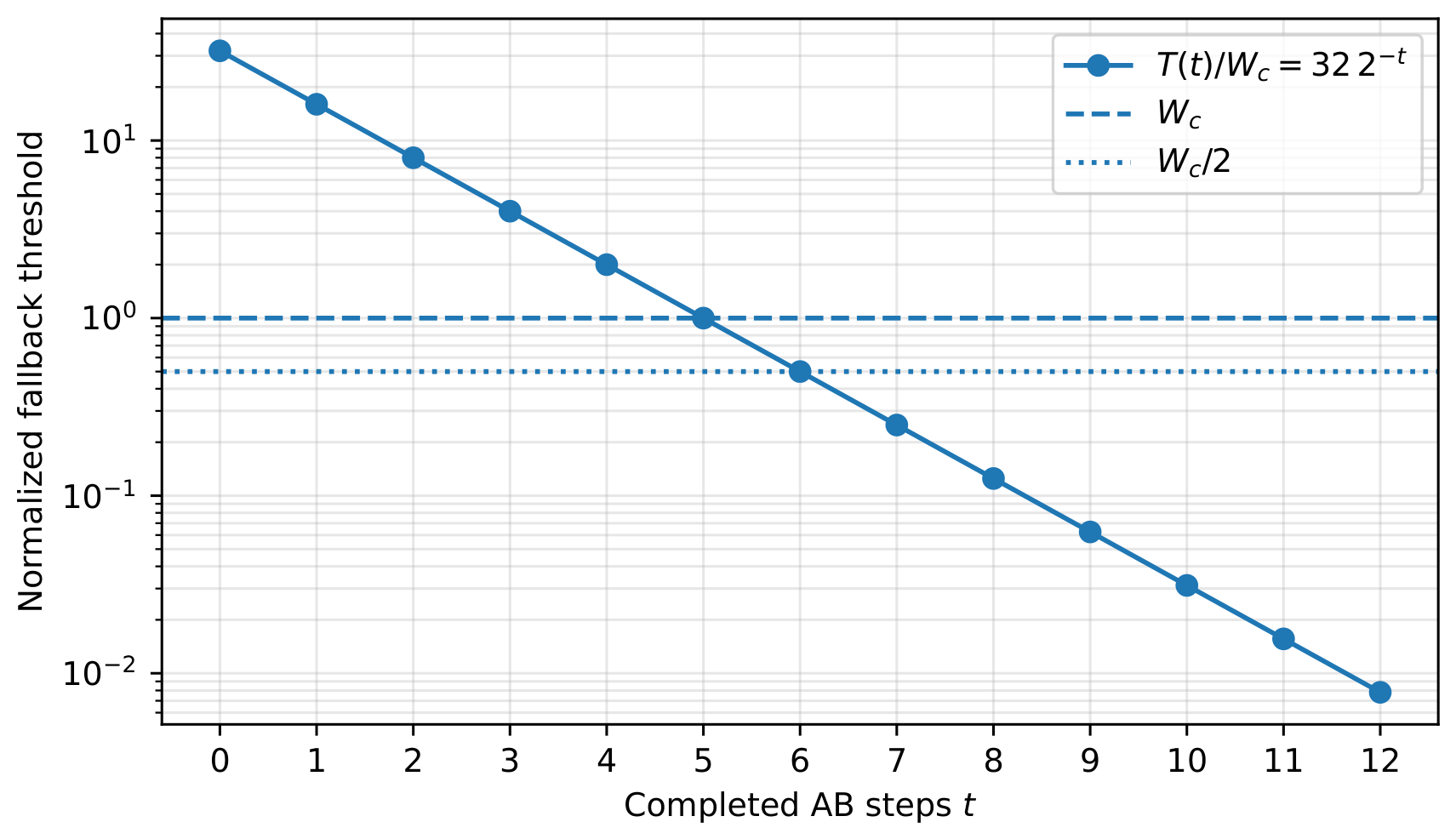
Table 1.
Shrinkage guaranteed by a completed phase block.
| AB steps t | Guaranteed halvings h | Iteration cost |
|---|---|---|
| 1 | ||
Table 2.
Eight ModAB changes and their purpose. C1–C6 identify the numbered comments in ModAB3C; S1–S2 identify those in ModAB3.
Table 2.
Eight ModAB changes and their purpose. C1–C6 identify the numbered comments in ModAB3C; S1–S2 identify those in ModAB3.
| No. | Comment | Change | Purpose |
|---|---|---|---|
| 1 | C1 | Store actual values of the function separately from AB modified ordinates. | Keep interpolation scaling separate from the actual function values. |
| 2 | C2 | Compute a finite trial point within the interval before forming the mixed tolerance. | Use a valid approximation in the relative tolerance term. |
| 3 | C3 | Reject a new NaN residual before sign decisions. | Exclude undefined values from sign comparisons. |
| 4 | C4 | Replace endpoints using the signs of the actual function value only. | Preserve the mathematical sign-changing bracket. |
| 5 | C5 | Restore modified ordinates from actual function values at fallback. | Initialize the next phase with the actual endpoint values. |
| 6 | C6 | Initialize the dyadic rule from the post-bisection width. | Retain , the five initially automatic comparisons, and the bound with . |
| 7 | S1 | Return a local function wrapper from Initialize. | Keep the function being evaluated local to each invocation. |
| 8 | S2 | Correct the description of side. | Document as a left-endpoint move and as a right-endpoint move. |
Table 3.
Function evaluations in the controlled C# comparison. Initial endpoint evaluations are included. Fixed and early variants change only the adaptive rule’s parameters.
Table 3.
Function evaluations in the controlled C# comparison. Initial endpoint evaluations are included. Fixed and early variants change only the adaptive rule’s parameters.
| Case or aggregate | Fixed delay | Early fallback | Adaptive |
|---|---|---|---|
| f64 | 9 | 14 | 9 |
| f84 | 9 | 16 | 9 |
| f92 | 24 | 21 | 21 |
| f93 | 23 | 21 | 21 |
| f94 | 24 | 21 | 21 |
| f95 | 22 | 19 | 19 |
| f96 | 23 | 20 | 20 |
| f97 | 24 | 21 | 21 |
| Raw sum, 92 reference-eligible cases | 1643 | 1658 | 1626 |
| Raw sum, common 89 validated cases | 1590 | 1605 | 1573 |
| Raw sum, 86 validated non-stress cases | 1492 | 1507 | 1475 |
| Penalized cost, 92 cases | 1758 | 1773 | 1741 |
Table 4.
C# results for the counterexample on . Restoring the exception cap changes termination, although the existing 100-case benchmark does not activate it.
Table 4.
C# results for the counterexample on . Restoring the exception cap changes termination, although the existing 100-case benchmark does not activate it.
| Rule | Solver status | Evaluations | Final width |
|---|---|---|---|
| Unlimited exceptions | MaxIterationsExceeded | 202 | 1 |
| Cap | Success | 77 |
Disclaimer/Publisher’s Note: The statements, opinions and data contained in all publications are solely those of the individual author(s) and contributor(s) and not of MDPI and/or the editor(s). MDPI and/or the editor(s) disclaim responsibility for any injury to people or property resulting from any ideas, methods, instructions or products referred to in the content. |
© 2026 by the authors. Licensee MDPI, Basel, Switzerland. This article is an open access article distributed under the terms and conditions of the Creative Commons Attribution (CC BY) license.
Copyright: This open access article is published under a Creative Commons CC BY 4.0 license, which permit the free download, distribution, and reuse, provided that the author and preprint are cited in any reuse.