

Submitted:
13 October 2026
Posted:
14 October 2026
You are already at the latest version
Abstract
Prostate cancer is the second most commonly diagnosed malignancy in men, yet interpretation of multiparametric MRI (mpMRI) suffers from substantial inter-observer variability and depends on scarce expert radiologists. Expert readers follow a hierarchical, coarse-to-fine visual strategy: they first localize the prostate gland and then direct focused attention to tissue within it. Inspired by this biological selective-attention mechanism, we propose a segmentation-guided framework in which a modality-aware 3D Vision Transformer (ViT) first delineates the prostate gland from T2-weighted, ADC, and DWI volumes, and the resulting anatomical mask then constrains downstream cancer detection. Global self-attention models long-range anatomical context, analogous to the integration of peripheral and foveal information in human vision. Detection was evaluated through two pathways: gray-level co-occurrence matrix (GLCM) texture features with classical classifiers, and a ViT classifier. On 200 patients from the public PROSTATEx cohort, the proposed segmentation model achieved a Dice similarity coefficient of [0.905] versus [0.831] for an optimized U-Net. The segmentation-guided ViT achieved an AUC of [0.987] and an accuracy of [0.998] for clinically significant cancer detection. Ablation experiments confirmed that anatomical guidance improved both pathways. These results show that emulating expert visual search strategies yields accurate and interpretable computer-aided prostate cancer diagnosis.
Keywords:
bioinspired attention
; vision transformer
; prostate cancer
; MRI segmentation
1. Introduction
Prostate cancer (PCa) is one of the most common cancers in men and remains a major global health concern. Early and accurate detection is important for clinical monitoring, treatment planning, and improved patient outcomes [1]. Over the past decade, many studies have explored PCa identification using statistical and machine learning (ML) methods. Although these methods have shown promise, their performance is often limited by simple model structures, small training datasets, and strong dependence on hand crafted features. As a result, their generalization ability remains limited [2]. More recent research has investigated advanced learning paradigms, including transfer learning and Vision Transformers (ViTs). ViTs analyze images through a self attention mechanism, which allows the model to focus on the most informative regions of the input and learn richer feature representations [2]. This is particularly useful in medical imaging, where annotated datasets are often limited. Transfer learning further improves this setting by allowing models pre trained on large datasets to transfer useful visual knowledge to the target task. This can improve diagnostic performance when task specific medical data are scarce [3].
Traditional ML methods, such as support vector machines (SVMs) and linear discriminant analysis (LDA), have also been applied to multiparametric magnetic resonance imaging (mpMRI) for prostate cancer detection. However, these approaches face two main limitations. First, they rely on manually designed features that may not capture the complex and heterogeneous patterns present in prostate MRI. Second, their classification performance is often insufficient for reliable clinical use [3]. Convolutional neural networks (CNNs) have improved many medical image analysis tasks, including segmentation and classification. Even so, they still have important limitations. CNNs mainly learn local spatial patterns and may not model long range anatomical dependencies effectively. This is a major issue in prostate MRI, where the shape of the gland, zonal structure, and broader anatomical context are important for diagnosis. Several extensions, such as larger kernels, deeper architectures, global pooling, dilated convolutions, and non local attention modules, have been proposed to address this problem. However, these solutions often increase model complexity.
ViTs provide a strong alternative. By replacing local convolution with global self attention, ViTs can capture relationships between distant image regions and model broader contextual information more effectively [4]. This property makes them attractive for prostate MRI analysis, where global anatomical context is important. Recent studies have reported encouraging results with ViT based models in several medical imaging tasks, including lung cancer detection from CT scans [5], multi label lung cancer classification from histopathological images [6] and prostate localization [7]. Despite these advances, important gaps remain. Most current studies treat prostate gland segmentation and cancer detection as separate tasks. As a result, the anatomical information learned during segmentation is not fully used to support the diagnosis. In addition, ViT based methods for prostate MRI are still limited, and their use in segmentation guided detection frameworks remains underexplored.
To address these limitations, this paper proposes a segmentation guided Vision Transformer framework for automated prostate cancer detection from mpMRI. The framework first uses a modality aware 3D ViT based model to segment the prostate gland and produce anatomically consistent prostate regions. These segmented regions are then used to guide downstream cancer detection.
The main contributions of this work are as follows:
- 1.
- We propose a segmentation-guided framework for automated prostate cancer detection from mpMRI.
- 2.
- We develop a modality aware 3D Vision Transformer model for prostate gland segmentation from volumetric mpMRI that captures long range anatomical context.
- 3.
- We use the segmented prostate region as an anatomical prior for downstream cancer detection.
- 4.
- We integrate segmentation-guided analysis with both conventional machine learning classifiers and a ViT-based detection model.
- 5.
- We demonstrate strong segmentation and detection performance on the publicly available dataset.
2. Related Work
Prostate cancer is one of the most frequently diagnosed cancers in men and remains a major cause of cancer related mortality worldwide [8]. For this reason, improving prostate cancer diagnosis has become an important research direction. In recent years, artificial intelligence and deep learning have attracted growing interest for prostate MRI analysis [9]. Several AI based strategies have been reported for prostate cancer detection. Yan et al. proposed a classifier based on pixel energy relationships [10]. Midiri et al. developed a computer aided detection system for MRI that identifies local maxima, extracts voxel level features, and segments the prostate using a multi atlas strategy [11]. They also used apparent diffusion coefficient (ADC) maps together with contrast and GLCM homogeneity features derived from T2-weighted images to estimate Gleason scores [12]. In another line of work, radiomic features have been studied using probabilistic support vector machines [13], while T2-weighted MRI has also been used in automatic pipelines for monitoring disease progression [14].
Other studies have explored texture analysis and conventional machine learning methods for prostate cancer assessment. Liu et al. extracted texture features such as energy, entropy, correlation, homogeneity, and inertia from MR images and analyzed them using generalized estimating equations [15]. Kong et al. compared traditional approaches with deep learning methods for prostate cancer detection and reported that GLCM with KNN Cosine was the strongest conventional method in their study [16]. These findings show that hand crafted texture descriptors remain useful, especially when combined with well established classifiers. However, their effectiveness still depends heavily on feature design and may be limited in more complex imaging settings. Deep learning has further improved automated prostate MRI analysis. Abbasi et al. proposed a three stage framework that included lesion localization, ADC normalization, and a stacked auto encoder with a non negativity constraint for prostate cancer detection [17]. Santhirasekaram et al. developed a computer aided diagnosis system using a deep CNN and biopsy defined points to identify prostate cancer from mpMRI [18]. Lopez et al. introduced a deep learning detection system that used filtered block samples for prostate localization [19]. Zavala Romero et al. combined instance and semantic segmentation to integrate local and global image features [20]. In addition, XmasNet used 3D rotation and slicing to better exploit volumetric mpMRI data for lesion analysis [21].
Several related studies have also focused on classification and multimodal analysis. Vos et al. proposed a two stage approach for benign and malignant classification [22]. Chung et al. used voxel level radiological features in a radiation driven framework for cancer detection [23]. Khalvati et al. performed feature selection across multiple MRI modalities and included texture based descriptors in their analysis [24]. Wang et al. later introduced a deformation network combined with multimodal registration for prostate cancer detection [25]. Although these studies have contributed valuable ideas, many of them still treat localization, segmentation, and diagnosis as separate components rather than as a unified framework. Beyond imaging methodology, epidemiological studies have shown that prostate cancer incidence increases markedly with age and rises sharply after the age of 40 [26]. Risk also varies across population groups. African American men face a substantially higher risk than Caucasian men [27], while Asian populations generally show lower incidence rates, although this pattern changes after migration to Western countries [28]. These findings highlight the broader clinical importance of accurate and robust diagnostic tools. Despite substantial progress, important limitations remain. Most existing methods treat prostate gland segmentation and cancer detection as separate tasks, which limits the use of anatomical information during diagnosis. In addition, CNN based models mainly learn local patterns and may not capture long range anatomical dependencies effectively. This is a major limitation in prostate MRI, where gland shape, zonal structure, and broader anatomical context are important. Vision Transformers have recently shown strong performance in medical imaging because of their global self attention mechanism. However, their application to prostate MRI remains limited, especially in segmentation-guided detection frameworks. Moreover, most transformer based studies focus on segmentation accuracy alone and do not examine how segmentation quality affects downstream cancer detection. These limitations motivate the present study, which develops a unified and anatomically informed framework for segmentation-guided prostate cancer detection from mpMRI.
Figure 1 illustrates the proposed framework. Raw mpMRI volumes are first pre-processed and then passed to the segmentation module. The resulting prostate masks are subsequently used to guide the final cancer detection stage.
3. Materials and Methods
3.1. Dataset Description
The PROSTATEx dataset, released by The Cancer Imaging Archive (TCIA), is a publicly available collection of prostate mpMRI studies developed for the SPIE-AAPM-NCI PROSTATEx grand challenge. It includes 346 patients and 349 prostate MRI scans, with imaging sequences such as T2-weighted (T2w), diffusion-weighted imaging (DWI) with apparent diffusion coefficient (ADC) maps, dynamic contrast-enhanced (DCE) imaging, and proton density-weighted images. The challenge framework defined 204 subjects for training and 140 for testing. Clinically significant prostate cancer was defined as biopsy-proven Gleason Grade Group . Owing to its rich multimodal imaging content, PROSTATEx has been widely used for both prostate cancer detection and segmentation research.
All images were acquired on Siemens 3T MRI scanners, including MAGNETOM Trio and Skyra systems. T2-weighted images were acquired using a turbo spin-echo sequence, with a slice thickness of 3.6 mm and an in-plane resolution of approximately 0.5 mm. DCE time series were acquired using a 3D turbo flash gradient-echo sequence, with a temporal resolution of 3.5 s, a slice thickness of 4 mm, and an in-plane resolution of approximately 1.5 mm. In this study, 200 patients were randomly selected from the PROSTATEx cohort for prostate gland segmentation [29]. Their mpMRI scans were acquired on Siemens 3T MRI scanners. The T2-weighted images had a slice thickness of 3.0 to 4.0 mm and an in-plane resolution of 0.3 to 0.7 mm. The most common resolution, seen in 74% of cases, was mm. The selected subset comprised 134 patients with clinically significant prostate cancer and 66 without clinically significant disease.
3.2. Preprocessing
All preprocessing steps were applied only after patient wise splitting into training, validation, and test subsets. This design prevented information leakage between subsets. During model development, prostate gland masks were used to localize the prostate region, thereby reducing computational cost and focusing the analysis on anatomically relevant tissue. Lesion level annotations were not used during preprocessing. Data augmentation was applied only to the training set in order to improve robustness and reduce overfitting. The validation and test sets were left unchanged to ensure an unbiased assessment of model performance.
3.2.1. Data Augmentation
Data augmentation was used to reduce overfitting and improve model robustness and generalization. In this study, a range of geometric and intensity-based transformations was applied to increase the diversity of training samples while preserving anatomical information. Flipping was used to reflect images along the horizontal or vertical axis [30]. Rotation introduced directional variation by transforming images through selected angles [31]. Shearing modified object shape by preserving one coordinate and shifting the other, while maintaining essential structural information [30]. Cropping was applied to simulate variation in the field of view while retaining relevant image content [31]. Translation repositioned objects without deformation, and the empty regions created during this process were filled with padding to avoid information loss [30].
Several contrast based augmentations were also employed. Gamma contrast adjusted brightness and contrast by varying the gamma value while preserving structural content. The gamma range was set from 0.5 to 2, with a probability of 0.2. Sigmoid contrast enhanced the dark and bright regions separately using a sigmoid intensity transformation, with the threshold coefficient set in the range 5 to 10 and a probability of 0.2. Linear contrast improved image uniformity by scaling intensities in a linear manner. Elastic transformation was used to simulate smooth deformations while preserving the identity and overall structure of the object.
Figure 2 shows representative examples of the augmentation methods applied during training.
3.2.2. Image Enhancement
Image enhancement was applied before feature extraction to improve image quality and increase the visibility of diagnostically relevant structures [32]. The following enhancement methods were used.
Brightness adjustment. Pixel intensities were adjusted using
where l is the lower pixel boundary, h is the upper boundary, n is the input value, o is the output value, c is the minimum output intensity, and d is the maximum output intensity. When the gamma value is greater than one, the image becomes darker, which can enhance contrast and highlight fine anatomical details [33]. However, excessive adjustment may introduce artifacts.
Gamma correction. A nonlinear intensity transformation was used to better match image brightness to the human visual response [34]:
Figure 3.
Effect of image enhancement methods on prostate MRI, including corresponding activation heatmaps. Brightness adjustment, gamma correction, and contrast stretching improve the visibility of anatomical structures compared with the original image.
Figure 3.
Effect of image enhancement methods on prostate MRI, including corresponding activation heatmaps. Brightness adjustment, gamma correction, and contrast stretching improve the visibility of anatomical structures compared with the original image.
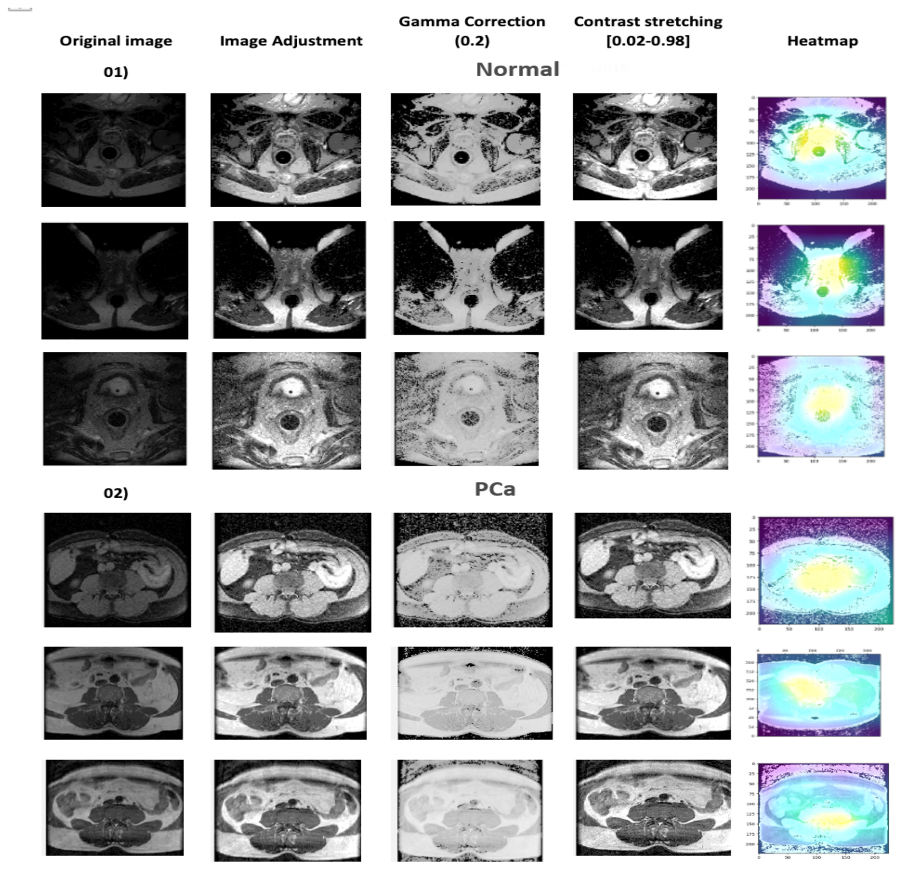
Contrast stretching. Intensity values were normalized to the range using
where denotes the desired output range and corresponds to the 5th and 95th percentile input intensities. Using percentile based limits reduces the influence of extreme outliers and improves contrast normalization [35].
3.3. Prostate Gland Segmentation
Prostate gland segmentation is a key component of the proposed framework. In this study, it serves as an anatomically informed intermediate step for downstream prostate cancer detection. Rather than analysing the full MRI volume directly, the framework first identifies the prostate gland and then uses this localized region to guide diagnosis. This design reduces the influence of irrelevant background structures and improves the anatomical focus of the detection stage. In medical imaging, segmentation tasks are commonly divided into semantic segmentation and instance segmentation. Semantic segmentation assigns a class label to each pixel or voxel, whereas instance segmentation additionally separates individual objects of the same class [36]. In the present study, prostate gland delineation is treated as a semantic segmentation problem. MRI provides the anatomical detail needed for this task and supports accurate gland level annotation [37]. Early deep learning-based segmentation methods relied on convolutional encoders to extract latent image representations [38]. More recent methods have extended this idea by incorporating stronger contextual modeling.
Figure 4 summarizes the feature categories relevant to anatomical segmentation. These include motion related information, appearance features, shape based constraints, and contextual relationships. In the present work, appearance is strengthened through image enhancement, while shape and context are modeled through the proposed segmentation framework. The aim is to produce anatomically consistent prostate gland masks that can serve as reliable inputs to the downstream cancer detection stage.
Figure 4.
Feature categories used for anatomical segmentation.
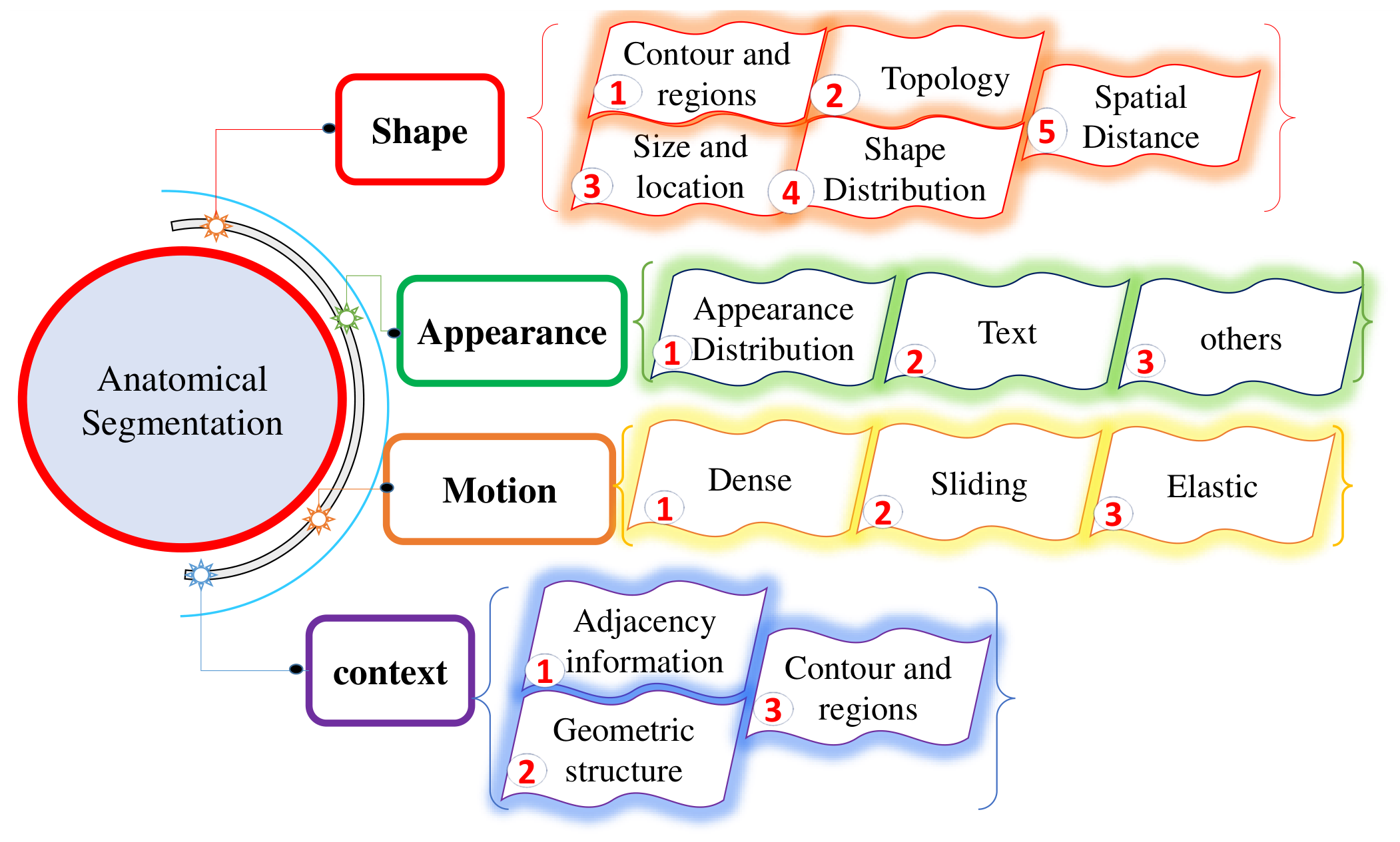
Figure 5.
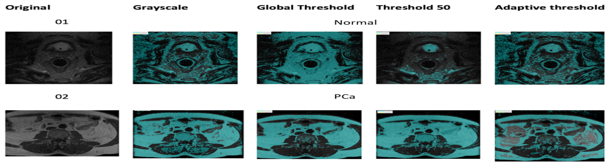
Prostate MRI segmentation using adaptive thresholding. Original and thresholded images are shown for both classes.
Figure 5.
Prostate MRI segmentation using adaptive thresholding. Original and thresholded images are shown for both classes.
3.4. Adaptive Thresholding
Global thresholding performs poorly when image contrast is non-uniform or the background lacks uniformity. Adaptive thresholding addresses this by computing local thresholds. A binary segmentation mask is defined as:
where is the locally computed threshold.
Figure 6.
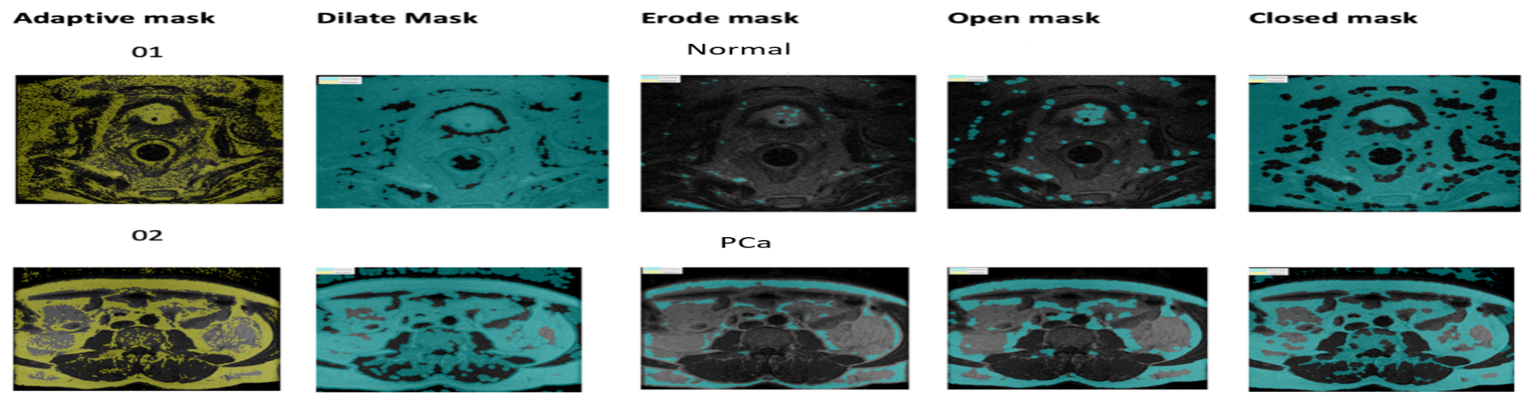
Prostate MRI segmentation using morphological operations. Original and post-morphology images are shown for both classes.
Figure 6.
Prostate MRI segmentation using morphological operations. Original and post-morphology images are shown for both classes.
3.5. Optimized U-Net Architecture
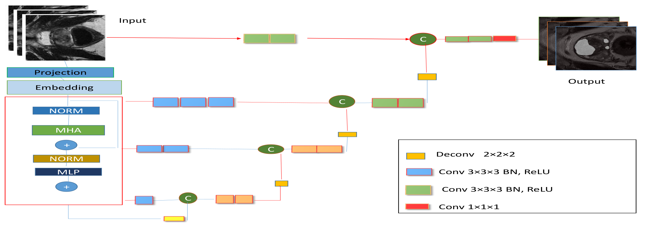
U-Net remains one of the most widely used architectures for medical image segmentation because it combines multi scale feature extraction with effective dense prediction. Its encoder captures local image patterns, while its decoder reconstructs spatial detail at the output resolution. However, convolutional operations mainly model local neighborhoods and may not capture long range anatomical dependencies effectively. This limitation is important in prostate MRI, where gland shape and broader anatomical context influence segmentation quality. For this reason, the optimized U-Net is used in this work as a strong baseline for comparison with the proposed transformer based segmentation model.
Figure 7.
Optimized U-Net architecture used for prostate gland segmentation.
3.6. Proposed Segmentation Model
The proposed segmentation model is designed to generate anatomically consistent prostate gland masks that can guide downstream cancer detection. Unlike conventional convolution based architectures, the proposed model uses modality aware inputs together with global self attention to capture long range anatomical dependencies in prostate MRI. This enables the network to model both local gland boundaries and broader contextual structure within the volume.
3.6.1. Problem Formulation
Given a multi-modal 3D prostate MRI volume:
where corresponds to the T2w, ADC, and DWI modalities, the objective is to predict a voxel wise binary segmentation mask: The segmentation model learns the mapping: where denotes trainable parameters. The mapping is optimized not only for voxel-level overlap but also to preserve the global anatomical coherence needed for reliable downstream cancer detection.
3.6.2. Input Normalization
Each modality is independently normalized using min max normalization:
3.6.3. Patch Embedding
The input volume is partitioned into non-overlapping 3D patches of size . The total number of patches is:
Each patch is projected into a latent embedding space of dimension E via a 3D convolution:
Learnable positional embeddings are added to preserve spatial ordering:
3.6.4. Transformer Encoder
Each transformer layer consists of a multi-head self attention (MHSA) block and a feed forward network (FFN).
Multi-Head Self-Attention.
Query, key, and value matrices are computed as:
Scaled dot-product attention is:
The MHSA output concatenates H attention heads:
A residual connection followed by layer normalization is applied:
Feed-Forward Network.
The FFN uses GELU activation: With a residual connection:
3.6.5. Decoder and Reconstruction
Transformer output tokens are reshaped into a 3D feature map: The decoder progressively upsamples to the original resolution: where denotes convolutional and transposed convolutional layers, and is the sigmoid activation function.
3.6.6. Loss Function
The total training loss is a sum of binary cross-entropy (BCE) loss and Dice loss:
Binary Cross-Entropy Loss.
Dice Loss.
3.6.7. Optimization
Model parameters are optimized using AdamW:
A warm up cosine learning rate schedule is used:
where is the peak learning rate, is the minimum learning rate, and is the normalized training progress after the warm-up phase. A linear warm-up over the first 5 epochs increases the learning rate from 0 to . Cosine annealing is applied for all remaining epochs.
Figure 8.
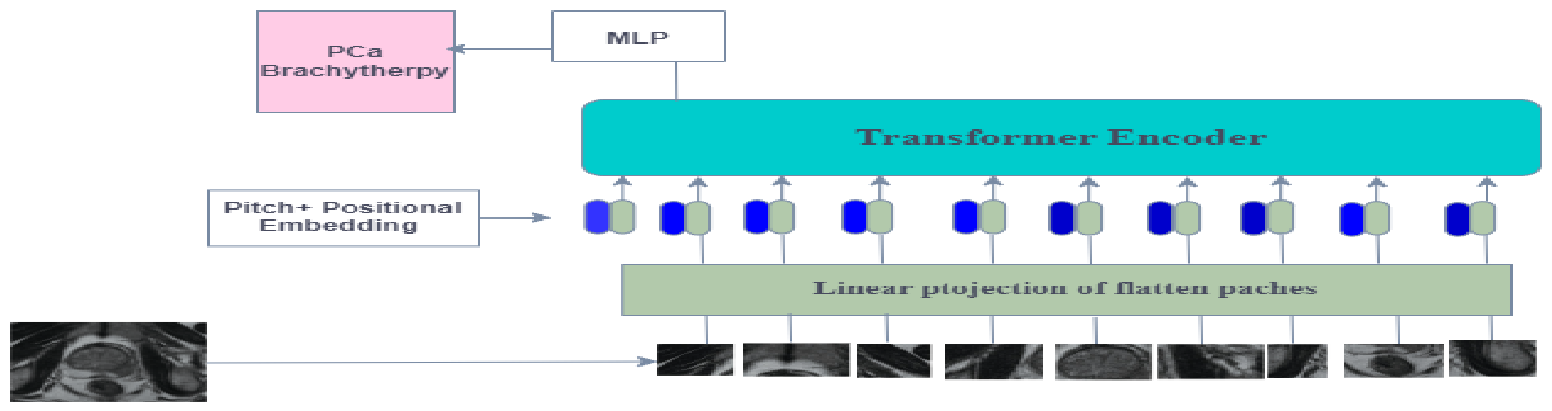
Vision Transformer (ViT) architecture used for prostate cancer detection.
4. Prostate Cancer Detection Methods
After segmentation, the localized prostate region is used for downstream cancer detection. Two complementary detection strategies are considered in this study. The first is a conventional machine learning pipeline based on hand crafted texture features. The second is a ViT based classifier. This dual evaluation makes it possible to assess the value of segmentation guided analysis across both classical and deep learning settings.
4.1. Feature-Based Machine Learning Pipeline
Classical machine learning approaches rely on hand crafted features extracted before classification. In this work, texture descriptors are computed from the segmented prostate region and then used to train established classifiers for cancer detection [39].
4.1.1. Feature Extraction
The textural properties of cancerous prostate tissue differ from those of normal tissue. Measures such as mean, standard deviation, and entropy are commonly used to capture these textural fluctuations. GLCM-based features are extracted following the method of Iqbal et al. [40].
Gray-Level Co-occurrence Matrix (GLCM) Features. Table 1 represents GLCM features. The GLCM encodes spatial co-occurrence statistics between pixel pairs and captures both spatial dependencies and textural correlations.
where is the mean intensity and , are standard deviations of the row and column marginal distributions.
4.1.2. Classifiers
Naive Bayes. The Naive Bayes classifier applies Bayes’ theorem under the assumption of feature independence. It estimates the posterior probability of each class given the observed features and selects the most probable class [41]. Despite its simplifying assumptions, Naive Bayes is computationally efficient and performs well across diverse medical datasets [42].
Decision Tree. Decision trees guide each sample through a series of attribute-based decisions toward a predicted class label [43]. They provide intuitive feature importance rankings, supporting dimensionality reduction as a preprocessing step.
4.2. Vision Transformer with Transfer Learning
The second detection branch uses a Vision Transformer based classifier. Transformers model long range dependencies through self attention and can therefore capture broader contextual relationships than purely local architectures. In this work, the ViT based classifier operates on the segmented prostate region and is used as the main deep learning detection model. Let be the input, where T denotes the number of tokens and C the embedding dimension. Query, key, and value projections are computed as:
where and . The attention output is:
The scaling factor prevents excessively small gradients in the softmax operation.
Positional information is encoded via sinusoidal embeddings:
where p is the token position and i the dimension index.
Multi-head attention extends single-head attention by projecting queries, keys, and values into multiple subspaces and concatenating their outputs. This allows the model to jointly attend to information from different representations sub-spaces at different positions.
5. Performance Measures
The following metrics were used to evaluate segmentation and classification performance.
5.1. Dice Similarity Coefficient (DSC)
The Dice Similarity Coefficient measures the spatial overlap between predicted and ground truth segmentation masks:
where TP, FP, and FN denote true positives, false positives, and false negatives, respectively.
5.2. Intersection over Union (IoU)
The IoU (Jaccard Index) measures the ratio of the intersection to the union of the predicted and ground truth regions []:
5.3. Precision
Precision (positive predictive value) measures the fraction of predicted positives that are truly positive:
5.4. F1-Score
The F1-score is the harmonic mean of precision and recall:
5.5. Receiver Operating Characteristic (ROC) Curve
The area under the ROC curve (AUC) summarizes classifier performance across all decision thresholds. An AUC of 1.0 indicates a perfect classifier; 0.5 indicates chance performance. AUC values in the range are generally considered excellent. The ROC metric is particularly informative for imbalanced datasets, as it evaluates both sensitivity (true positive rate) and specificity (1 − false positive rate) [].
5.6. Implementation Details
All experiments were conducted on a workstation equipped with an 11th generation Intel Corei9-11900KF processor (3.50GHz), 64GB of system RAM, and an NVIDIA GeForce RTX 3060 GPU with 12 GB of dedicated memory. The framework was implemented in PyTorch. Standard scientific computing libraries (NumPy, Pandas, Nibabel) were used for handling volumetric MRI data. The model uses a 3D ViT-based encoder–decoder architecture. Input volumes were resized to voxels. The patch embedding module divides the volume into non-overlapping patches, which are projected into a 192-dimensional embedding space. The transformer encoder comprises 12 layers with 6 self attention heads and a feed forward expansion ratio of 4.0. Positional embeddings are learned. The decoder reconstructs the segmentation map using convolutional and transposed convolutional layers. The model is trained with a combined Dice + BCE loss. A batch size of 2 and gradient accumulation of 2 steps yield an effective batch size of 4. Optimization uses AdamW with and weight decay . The learning rate follows a warm-up cosine schedule over 100 epochs (5 warm-up epochs, minimum learning rate ).
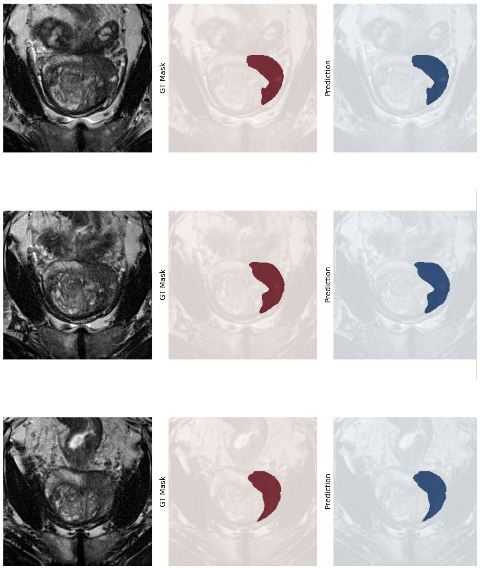
Figure 9.
Visual comparison of original image, ground truth mask, and the predicted mask produced by the proposed 3D ViT segmentation model. Row 1: The predicted mask captures the overall shape of the prostate gland but slightly overestimates its extent on the left. Row 2: The predicted mask aligns closely with the ground truth, with only minor discrepancies at fine boundary details.
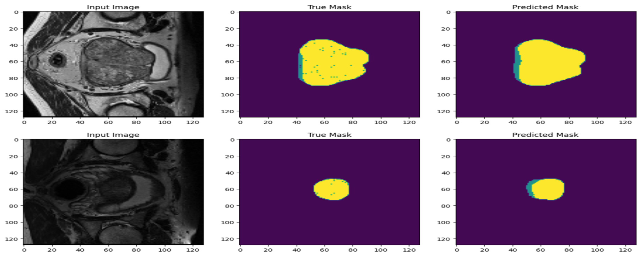
Figure 10.
Training curves of the optimized U-Net model: accuracy and Dice coefficient versus epoch. Both metrics increase steadily and stabilize after approximately epoch 100, indicating convergence.
Figure 10.
Training curves of the optimized U-Net model: accuracy and Dice coefficient versus epoch. Both metrics increase steadily and stabilize after approximately epoch 100, indicating convergence.
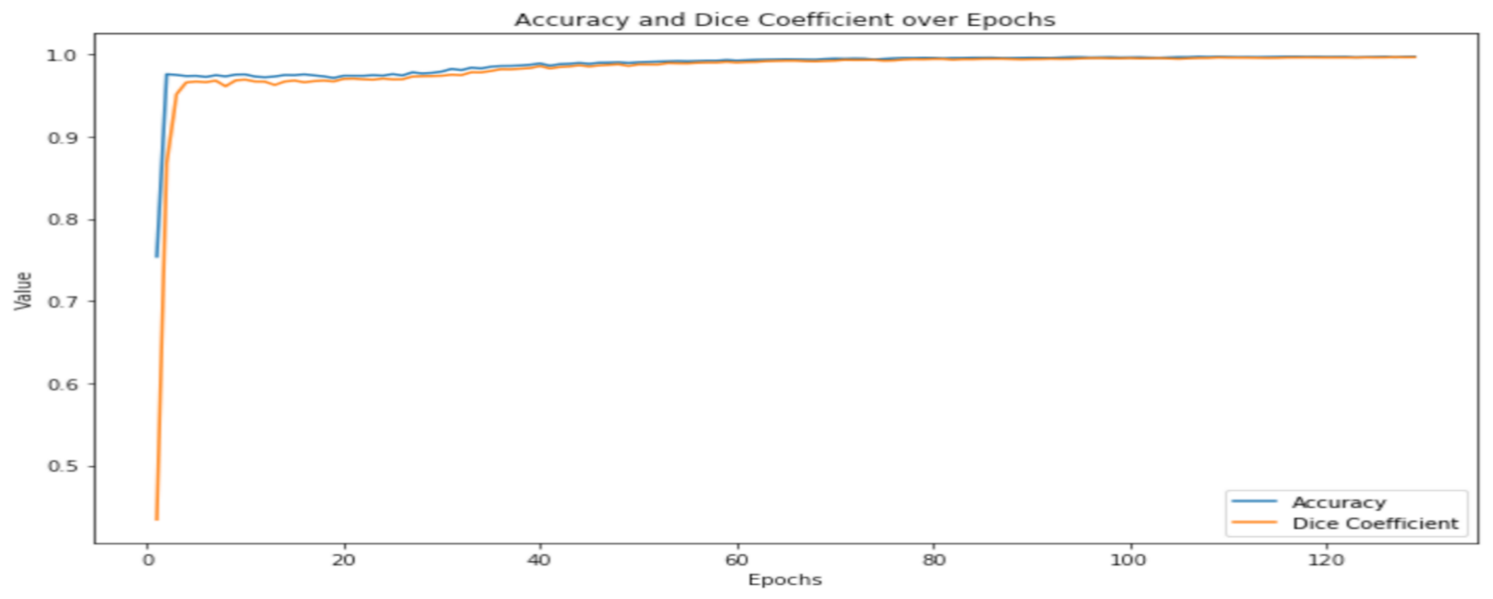
Figure 11.
Overlay visualization of the ground truth mask and predicted mask from the proposed 3D ViT segmentation model on a representative case.
Figure 11.
Overlay visualization of the ground truth mask and predicted mask from the proposed 3D ViT segmentation model on a representative case.
6. Results and Discussion
Table 2 and Table 3 summarize the segmentation results. The proposed model achieves a Dice score of 0.9048 and an IoU of 0.728, indicating substantial overlap with the ground truth masks. Precision (0.889) and recall (0.803) are well balanced, indicating good control over both false positives and false negatives. Boundary fidelity is confirmed by a Hausdorff Distance of 2.11mm and an Average Surface Distance of 3.31mm. High ROC-AUC (0.987) and PR-AUC (0.928) further confirm robust pixel-level discriminative capacity. All metrics exceed those of the optimized U-Net baseline, demonstrating the benefit of incorporating global self-attention into the segmentation architecture.
6.1. Cancer Detection Performance
Both deep and classical classifiers were evaluated: SVM with radial basis function (RBF) kernel, Naive Bayes, RUSBoosted Tree, Decision Tree, and the proposed ViT with transfer learning. A patient-wise split was enforced throughout to prevent data leakage and ensure unbiased evaluation on entirely unseen patients.
Figure 12 summarizes the detection performance of the evaluated classifiers. The proposed ViT based classifier achieves the strongest overall balance across sensitivity, specificity, PPV, NPV, precision, and accuracy, indicating reliable discrimination between cancer and non cancer cases within the segmented prostate region. Some conventional classifiers achieve slightly higher AUC values, showing that they remain competitive in ranking performance. Overall, however, the proposed segmentation guided ViT pipeline provides the most consistent detection performance across the broader set of reported evaluation measures.
Table 4 reports per class classification results for the ViT model with adaptive thresholding and morphological preprocessing. The model achieves 99.8% overall accuracy and balanced performance across both classes. Precision of 0.998 indicates that nearly all predicted positive cases are true positives. A recall of 0.987 indicates that the model misses very few genuine PCa cases. The F1 score of 0.987 for the PCa class reflects a good balance between precision and recall. These characteristics are important for clinical deployment, where both false positives and false negatives carry significant consequences.
Figure 13.
ROC curve for prostate cancer detection using the proposed 3D ViT segmentation-guided model. The AUC of 0.987 indicates excellent discriminative performance.
Figure 13.
ROC curve for prostate cancer detection using the proposed 3D ViT segmentation-guided model. The AUC of 0.987 indicates excellent discriminative performance.
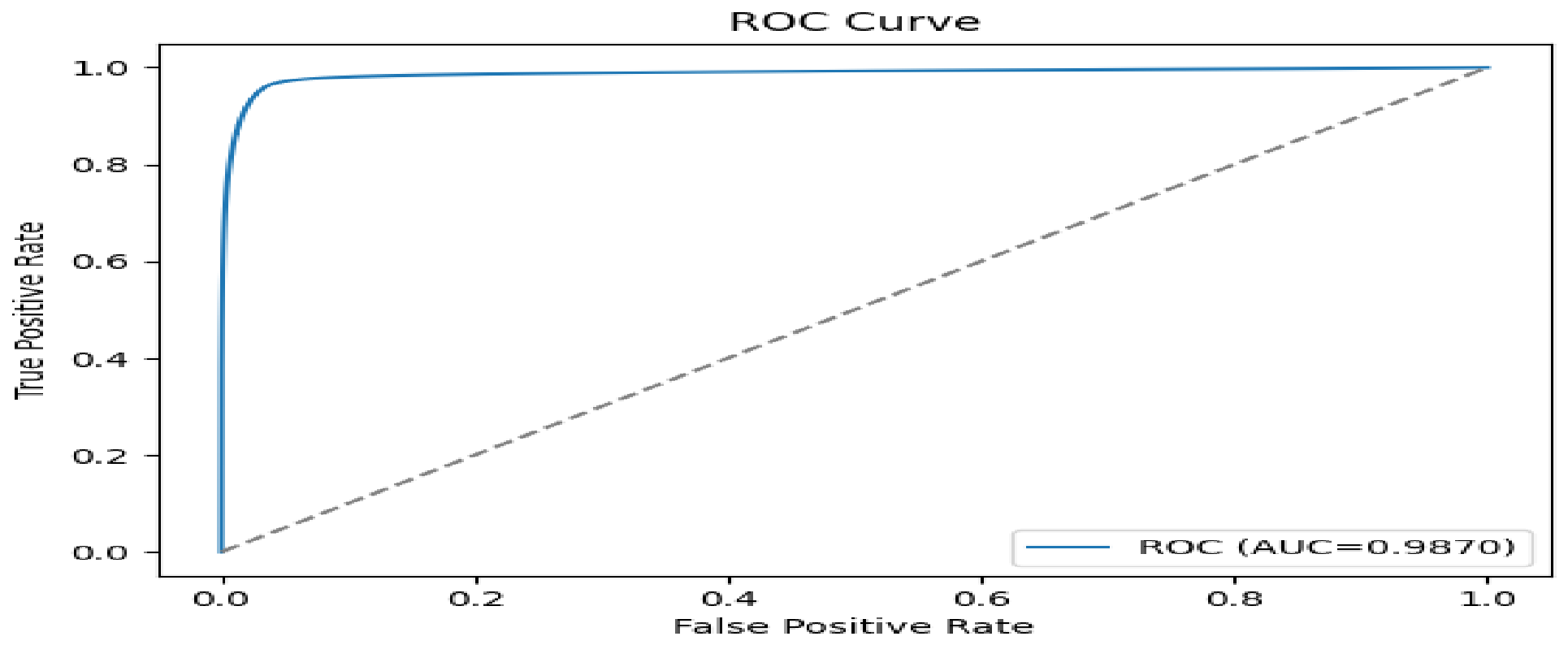
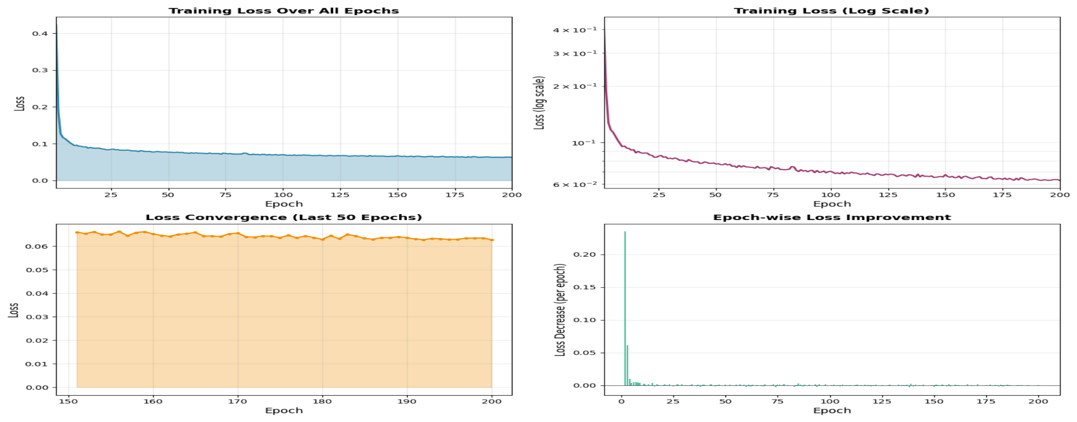
Figure 14.
Training loss curve of the proposed segmentation model over 200 epochs. Loss decreases rapidly in the early epochs as the model learns coarse anatomical and prostate structures, followed by a gradual, stable decline. The logarithmic scale reveals continued optimization at later epochs. Convergence is confirmed by minor fluctuations in the final 50 epochs.
6.2. Ablation Study
Table 5 presents the ablation results. Each added component improves overall performance. Preprocessing and augmentation increase the AUC from 0.850 to 0.880. Adding segmentation guidance further improves the AUC to 0.900 and yields a Dice score of 0.900. The full model achieves the best overall performance, indicating that segmentation guidance, preprocessing, and augmentation each contribute to the final result.
6.3. Comparison with State of the Art
Table 6 compares the proposed method with recent published work. Hussain et al. achieved AUC = 0.99 using morphological and SIFT features [48]. Jung et al. reported AUC = 0.90 with a radiomics-only approach [49]. Ali et al. obtained DSC = 0.80 for volumetric segmentation on two datasets [50]. Giganti et al.reported AUC = 0.85 with a combined CAD and deep learning system [51]. The proposed framework achieves a Dice score of 0.905 and a detection AUC of 0.987, which are competitive with those reported in the literature while also providing explicit segmentation guidance. The proposed method offers the additional advantage of integrating prostate gland segmentation directly into the detection pipeline, thereby improving anatomical focus and strengthening its relevance to clinically meaningful mpMRI analysis. Regarding computational characteristics: ViT uses a self attention mechanism that scales linearly with the number of patches for large images, whereas ResNet101 scales quadratically with image size due to its convolutional operations [39,52]. ViT primarily stores the attention matrix, and optimizations such as relative attention and windowed attention significantly reduce its memory footprint [53]. This makes ViT is more scalable for high-resolution volumetric inputs such as prostate mpMRI.
7. Conclusion and Limitations
This study proposed a segmentation guided Vision Transformer framework for automated prostate cancer detection from multiparametric MRI. The framework first segments the prostate gland and then uses the segmented prostate region to guide downstream cancer detection. By combining anatomical localization with diagnostic prediction, the proposed method improves the anatomical focus of the detection stage and captures long range contextual information that is difficult to model with conventional convolution based approaches. Experimental results on the publicly available PROSTATEx dataset showed strong segmentation performance and high downstream detection performance. The findings suggest that anatomically guided analysis can improve the reliability of automated interpretation of prostate MRI by reducing the influence of irrelevant background structures. These results support the value of combining prostate segmentation with transformer based global contextual modeling for computer aided prostate cancer diagnosis. This study also has important limitations. The framework was evaluated on a single publicly available dataset, and broader validation is needed to assess generalizability across institutions, scanner settings, and imaging protocols. In addition, the current method focuses on prostate gland segmentation and does not include lesion level segmentation. Future work will therefore examine multi center validation, integration of clinical variables, lesion level analysis, and improvements in computational efficiency for clinical deployment.
Data Availability Statement
The data supporting the findings of this study are available from the corresponding author upon reasonable request.
Conflicts of Interest
The authors declare that they have no conflict of interest.
References
- Bray, F.; Ferlay, J.; Soerjomataram, I.; Siegel, R.L.; Torre, L.A.; Jemal, A. Global cancer statistics 2018: GLOBOCAN estimates of incidence and mortality worldwide for 36 cancers in 185 countries. CA: a cancer journal for clinicians 2018, 68, 394–424.
- Litjens, G.; Debats, O.; Barentsz, J.; Karssemeijer, N.; Huisman, H. Computer-aided detection of prostate cancer in MRI. IEEE transactions on medical imaging 2014, 33, 1083–1092.
- Fehr, D.; Veeraraghavan, H.; Wibmer, A.; Gondo, T.; Matsumoto, K.; Vargas, H.A.; Sala, E.; Hricak, H.; Deasy, J.O. Automatic classification of prostate cancer Gleason scores from multiparametric magnetic resonance images. Proceedings of the National Academy of Sciences 2015, 112, E6265–E6273.
- Dosovitskiy, A.; Beyer, L.; Kolesnikov, A.; Weissenborn, D.; Zhai, X.; Unterthiner, T.; Dehghani, M.; Minderer, M.; Heigold, G.; Gelly, S.; et al. An image is worth 16x16 words: Transformers for image recognition at scale. arXiv preprint arXiv:2010.11929 2020.
- Ali, H.; Mohsen, F.; Shah, Z. Improving diagnosis and prognosis of lung cancer using vision transformers: a scoping review. BMC Medical Imaging 2023, 23, 129.
- Zhang, S.; Xu, Y.; Usuyama, N.; Bagga, J.; Tinn, R.; Preston, S.; Rao, R.; Wei, M.; Valluri, N.; Wong, C.; et al. Large-scale domain-specific pretraining for biomedical vision-language processing. arXiv preprint arXiv:2303.00915 2023, 2, 6.
- Paudyal, R.; Shah, A.D.; Akin, O.; Do, R.K.; Konar, A.S.; Hatzoglou, V.; Mahmood, U.; Lee, N.; Wong, R.J.; Banerjee, S.; et al. Artificial intelligence in CT and MR imaging for oncological applications. Cancers 2023, 15, 2573.
- Wang, C.; Zhang, Y.; Gao, W.Q. The evolving role of immune cells in prostate cancer. Cancer letters 2022, 525, 9–21.
- Guo, Y.; Zhong, L.; Min, L.; Wang, J.; Wu, Y.; Chen, K.; Wei, K.; Rao, C. Adaptive optics based on machine learning: a review. Opto-Electronic Advances 2022, 5, 200082–1.
- Yan, F.; Huang, H.; Pedrycz, W.; Hirota, K. Automated breast cancer detection in mammography using ensemble classifier and feature weighting algorithms. Expert Systems with Applications 2023, 227, 120282.
- Midiri, F.; Vernuccio, F.; Purpura, P.; Alongi, P.; Bartolotta, T.V. Multiparametric MRI and radiomics in prostate cancer: a review of the current literature. Diagnostics 2021, 11, 1829.
- Thanapandiyaraj, R.; Rajendran, T.; Mohammedgani, P.B. Performance analysis of various nanocontrast agents and CAD systems for cancer diagnosis. Current Medical Imaging Reviews 2019, 15, 831–852.
- Giannini, V.; Vignati, A.; Mirasole, S.; Mazzetti, S.; Russo, F.; Stasi, M.; Regge, D. MR-T2-weighted signal intensity: a new imaging biomarker of prostate cancer aggressiveness. Computer Methods in Biomechanics and Biomedical Engineering: Imaging & Visualization 2016, 4, 130–134.
- Nagarajan, M.B.; Raman, S.S.; Lo, P.; Lin, W.C.; Khoshnoodi, P.; Sayre, J.W.; Ramakrishna, B.; Ahuja, P.; Huang, J.; Margolis, D.J.; et al. Building a high-resolution T2-weighted MR-based probabilistic model of tumor occurrence in the prostate. Abdominal Radiology 2018, 43, 2487–2496.
- Liu, S.; Zheng, H.; Feng, Y.; Li, W. Prostate cancer diagnosis using deep learning with 3D multiparametric MRI. In Proceedings of the Medical imaging 2017: computer-aided diagnosis. SPIE, 2017, Vol. 10134, pp. 581–584.
- Kong, Q.; Xu, Y.; Wang, W.; Plumbley, M.D. Sound event detection of weakly labelled data with cnn-transformer and automatic threshold optimization. IEEE/ACM Transactions on Audio, Speech, and Language Processing 2020, 28, 2450–2460.
- Abbasi, A.A.; Hussain, L.; Awan, I.A.; Abbasi, I.; Majid, A.; Nadeem, M.S.A.; Chaudhary, Q.A. Detecting prostate cancer using deep learning convolution neural network with transfer learning approach. Cognitive Neurodynamics 2020, 14, 523–533.
- Santhirasekaram, A.; Pinto, K.; Winkler, M.; Aboagye, E.; Glocker, B.; Rockall, A. Multi-scale Hybrid transformer networks: application to prostate disease classification. In Proceedings of the International workshop on multimodal learning for clinical decision support. Springer, 2021, pp. 12–21.
- Duran-Lopez, L.; Dominguez-Morales, J.P.; Conde-Martin, A.F.; Vicente-Diaz, S.; Linares-Barranco, A. PROMETEO: A CNN-Based Computer-Aided Diagnosis System for WSI Prostate Cancer Detection. IEEE Access 2020, 8, 128613–128628. [CrossRef]
- Zavala-Romero, O.; Breto, A.L.; Xu, I.R.; Chang, Y.C.C.; Gautney, N.; Dal Pra, A.; Abramowitz, M.C.; Pollack, A.; Stoyanova, R. Segmentation of prostate and prostate zones using deep learning: A multi-MRI vendor analysis. Strahlentherapie und Onkologie 2020, 196, 932–942 . [CrossRef]
- Perez, I.M.; Toivonen, J.; Movahedi, P.; Merisaari, H.; Pesola, M.; Taimen, P.; Boström, P.J.; Kiviniemi, A.; Aronen, H.J.; Pahikkala, T.; et al. Diffusion weighted imaging of prostate cancer: prediction of cancer using texture features from parametric maps of the monoexponential and kurtosis functions. In Proceedings of the 2016 Sixth International Conference on Image Processing Theory, Tools and Applications (IPTA). IEEE, 2016, pp. 1–6.
- Vos, P.C.; Barentsz, J.O.; Karssemeijer, N.; Huisman, H.J. Automatic computer-aided detection of prostate cancer based on multiparametric magnetic resonance image analysis. Physics in Medicine and Biology 2012, 57, 1527–1542. [CrossRef]
- Chung, A.G.; Khalvati, F.; Shafiee, M.J.; Haider, M.A.; Wong, A. Prostate Cancer Detection via a Quantitative Radiomics-Driven Conditional Random Field Framework. IEEE Access 2015, 3, 2531–2541. [CrossRef]
- Khalvati, F.; Wong, A.; Haider, M.A. Automated prostate cancer detection via comprehensive multi-parametric magnetic resonance imaging texture feature models. BMC Medical Imaging 2015, 15. [CrossRef]
- Wang, Z.; Zhang, X.; Wang, X.; Zhang, L. Enhanced multi-modal abdominal image registration via structural awareness and region-specific optimization. Pattern Recognition Letters 2025, 188, 29–36.
- Morozov, A.; Taratkin, M.; Bazarkin, A.; Rivas, J.G.; Puliatti, S.; Checcucci, E.; Belenchon, I.R.; Kowalewski, K.F.; Shpikina, A.; Singla, N.; et al. A systematic review and meta-analysis of artificial intelligence diagnostic accuracy in prostate cancer histology identification and grading. Prostate cancer and prostatic diseases 2023, 26, 681–692.
- Jang, A.; Lanka, S.M.; Huang, M.; Casado, C.V.; Caputo, S.A.; Sweeney, P.L.; Gupta, K.; Pocha, O.; Habibian, N.; Hawkins, M.E.; et al. Comparison of circulating tumor DNA between African American and Caucasian patients with metastatic castrate-resistant prostate cancer post-abiraterone and/or enzalutamide. The Prostate 2023, 83, 1028–1034.
- Ito, K.; Kimura, T. Complex epidemiology of prostate cancer in Asian countries. Journal of Urologic Oncology 2023, 21, 5–13.
- Holmlund, W.; Simkó, A.; Söderkvist, K.; Palásti, P.; Tótin, S.; Kalmár, K.; Domoki, Z.; Fejes, Z.; Kincses, Z.T.; Brynolfsson, P.; et al. ProstateZones–Segmentations of the prostatic zones and urethra for the PROSTATEx dataset. Scientific Data 2024, 11, 1097.
- Vyas, A.; Yu, S.; Paik, J., Fundamentals of Digital Image Processing. In Multiscale Transforms with Application to Image Processing; Springer Singapore, 2017; p. 3–11. [CrossRef]
- Sifre, L.; Mallat, S. Rotation, Scaling and Deformation Invariant Scattering for Texture Discrimination. In Proceedings of the 2013 IEEE Conference on Computer Vision and Pattern Recognition. IEEE, 2013. [CrossRef]
- Soliman, S.R.; Zayed, H.H.; Selim, M.M.; Kasban, H.; Mongy, T. Image quality enhancement in Neutron Computerized Tomography based on projection exposure time adjustment. Applied Radiation and Isotopes 2019, 154, 108862. [CrossRef]
- Paul, E.M.; Perumal, B.; Rajasekaran, M.P. Filters Used in X-Ray Chest Images for Initial Stage Tuberculosis Detection. In Proceedings of the 2018 International Conference on Inventive Research in Computing Applications (ICIRCA). IEEE, 2018, p. 235–239. [CrossRef]
- Tiwari, M.; Gupta, B. Brightness preserving contrast enhancement of medical images using adaptive gamma correction and homomorphic filtering. In Proceedings of the 2016 IEEE Students’ Conference on Electrical, Electronics and Computer Science (SCEECS). IEEE, 2016, p. 1–4. [CrossRef]
- Hongjuan, Y.; Decai, M.; Yunchu, Z.; jianrong, C. Preprocessing of automobile engine connecting rod based on shadow removal and image enhancement. In Proceedings of the 2021 International Conference on Communications, Information System and Computer Engineering (CISCE). IEEE, 2021, p. 428–432. [CrossRef]
- Minaee, S.; Boykov, Y.Y.; Porikli, F.; Plaza, A.J.; Kehtarnavaz, N.; Terzopoulos, D. Image Segmentation Using Deep Learning: A Survey. IEEE Transactions on Pattern Analysis and Machine Intelligence 2021, p. 1–1. [CrossRef]
- Wu, E.; Wu, K.; Daneshjou, R.; Ouyang, D.; Ho, D.E.; Zou, J. How medical AI devices are evaluated: limitations and recommendations from an analysis of FDA approvals. Nature Medicine 2021, 27, 582–584. [CrossRef]
- Giusti, A.; Ciresan, D.C.; Masci, J.; Gambardella, L.M.; Schmidhuber, J. Fast image scanning with deep max-pooling convolutional neural networks. In Proceedings of the 2013 IEEE International Conference on Image Processing. IEEE, 2013. [CrossRef]
- Hatamizadeh, A.; Tang, Y.; Nath, V.; Yang, D.; Myronenko, A.; Landman, B.; Roth, H.R.; Xu, D. UNETR: Transformers for 3D Medical Image Segmentation. In Proceedings of the 2022 IEEE/CVF Winter Conference on Applications of Computer Vision (WACV). IEEE, 2022, p. 1748–1758. [CrossRef]
- Iqbal, S.; Siddiqui, G.F.; Rehman, A.; Hussain, L.; Saba, T.; Tariq, U.; Abbasi, A.A. Prostate cancer detection using deep learning and traditional techniques. Ieee Access 2021, 9, 27085–27100.
- Jiang, L.; Cai, Z.; Zhang, H.; Wang, D. Naive Bayes text classifiers: a locally weighted learning approach. Journal of Experimental & Theoretical Artificial Intelligence 2013, 25, 273–286. [CrossRef]
- Li, M.; Chen, T.; Zhao, W.; Wei, C.; Li, X.; Duan, S.; Ji, L.; Lu, Z.; Shen, J. Radiomics prediction model for the improved diagnosis of clinically significant prostate cancer on biparametric MRI. Quantitative Imaging in Medicine and Surgery 2020, 10, 368–379. [CrossRef]
- Charbuty, B.; Abdulazeez, A. Classification Based on Decision Tree Algorithm for Machine Learning. Journal of Applied Science and Technology Trends 2021, 2, 20–28. [CrossRef]
- Abu Al-Haija, Q.; Krichen, M.; Abu Elhaija, W. Machine-Learning-Based Darknet Traffic Detection System for IoT Applications. Electronics 2022, 11, 556. [CrossRef]
- Sahlaoui, H.; Alaoui, E.A.A.; Agoujil, S.; Nayyar, A. An empirical assessment of smote variants techniques and interpretation methods in improving the accuracy and the interpretability of student performance models. Education and Information Technologies 2023, 29, 5447–5483. [CrossRef]
- Wernick, M.; Yang, Y.; Brankov, J.; Yourganov, G.; Strother, S. Machine Learning in Medical Imaging. IEEE Signal Processing Magazine 2010, 27, 25–38. [CrossRef]
- Manhas, J.; Gupta, R.K.; Roy, P.P. A Review on Automated Cancer Detection in Medical Images using Machine Learning and Deep Learning based Computational Techniques: Challenges and Opportunities. Archives of Computational Methods in Engineering 2021, 29, 2893–2933. [CrossRef]
- Hussain, L.; Ahmed, A.; Saeed, S.; Rathore, S.; Awan, I.A.; Shah, S.A.; Majid, A.; Idris, A.; Awan, A.A. Prostate cancer detection using machine learning techniques by employing combination of features extracting strategies. Cancer Biomarkers 2018, 21, 393–413.
- Jung, S.; Kim, J.S. Radiomics Reproducibility in Prostate Cancer Diagnosis Based on PROSTATEx. International Neurourology Journal 2025, 29, S95.
- Ali, M.; Nassrullah, H.A.A.; Mohammed, Z.I.; Mohammad, S.J.; Salman, Z.N.; Abdullah, A.S.; Hussein, R.M. Prostate Cancer Volume Segmentation in Multiparametric MRI Scans Using Optimized 3D Dense CNN Architectures. In Proceedings of the 2025 3rd International Conference on Cyber Resilience (ICCR). IEEE, 2025, pp. 1–8.
- Giganti, F.; Moreira da Silva, N.; Yeung, M.; Davies, L.; Frary, A.; Ferrer Rodriguez, M.; Sushentsev, N.; Ashley, N.; Andreou, A.; Bradley, A.; et al. AI-powered prostate cancer detection: a multi-centre, multi-scanner validation study. European Radiology 2025, 35, 4915–4924.
- Jusman, Y. Comparison of prostate cell image classification using cnn: Resnet-101 and vgg-19. In Proceedings of the 2023 IEEE 13th International Conference on Control System, Computing and Engineering (ICCSCE). IEEE, 2023, pp. 74–78.
- Pan, Z.; Zhuang, B.; Liu, J.; He, H.; Cai, J. Scalable Vision Transformers with Hierarchical Pooling. In Proceedings of the 2021 IEEE/CVF International Conference on Computer Vision (ICCV). IEEE, 2021. [CrossRef]
- Al-Zidi, N.M.; Vasumathi, D. Synergistic Integration of Radiomics and Deep Features from Multiparametric MRI for Enhanced Prostate Cancer Classification. International Journal of Intelligent Engineering & Systems 2026, 19.
Figure 1.
Schematic diagram of the proposed prostate cancer detection framework. The pipeline takes PROSTATEx mpMRI images as input, applies preprocessing, performs prostate gland segmentation with the proposed 3D ViT model, and then performs cancer detection.
Figure 1.
Schematic diagram of the proposed prostate cancer detection framework. The pipeline takes PROSTATEx mpMRI images as input, applies preprocessing, performs prostate gland segmentation with the proposed 3D ViT model, and then performs cancer detection.
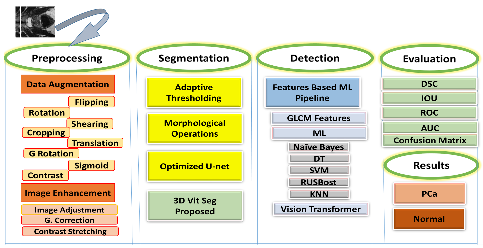
Figure 2.
Augmentation techniques applied to representative prostate MRI images.
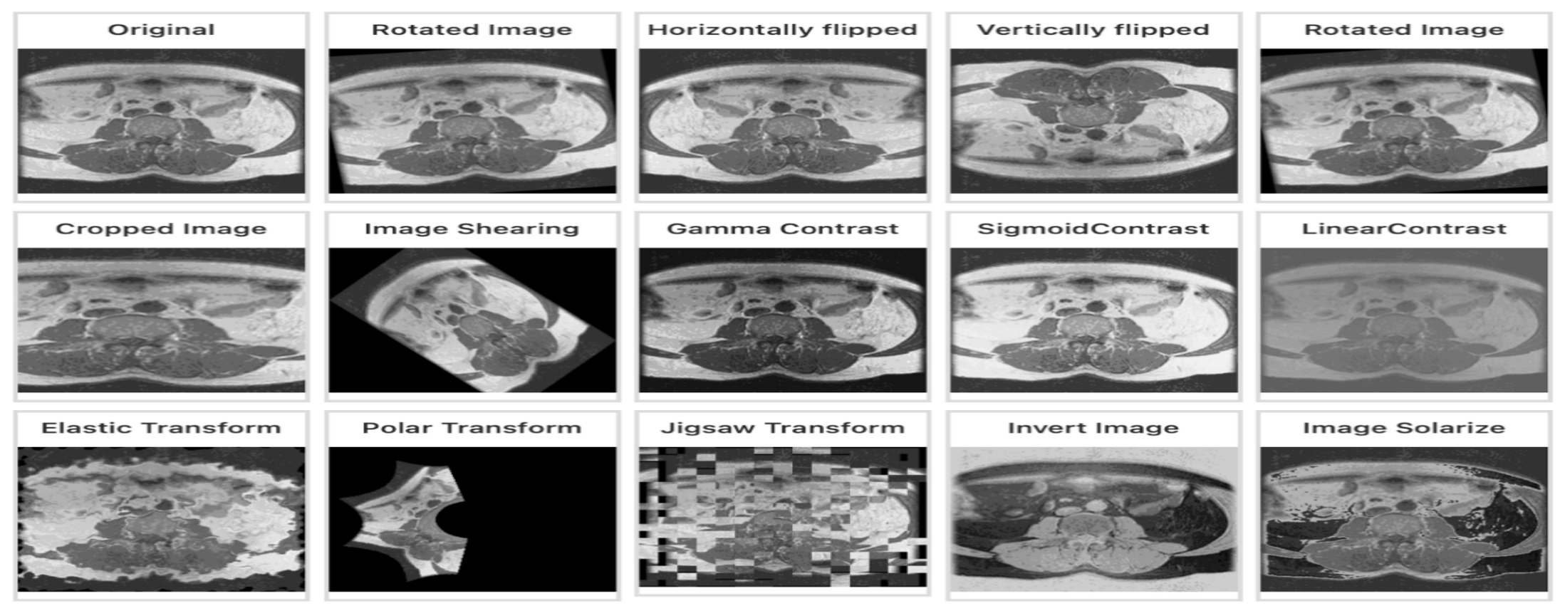
Figure 12.
Comparative detection performance of six classifiers using GLCM based features and ViT based transfer learning in the initial classifier comparison setting. Metrics shown are sensitivity, specificity, PPV, NPV, precision, and AUC.
Figure 12.
Comparative detection performance of six classifiers using GLCM based features and ViT based transfer learning in the initial classifier comparison setting. Metrics shown are sensitivity, specificity, PPV, NPV, precision, and AUC.
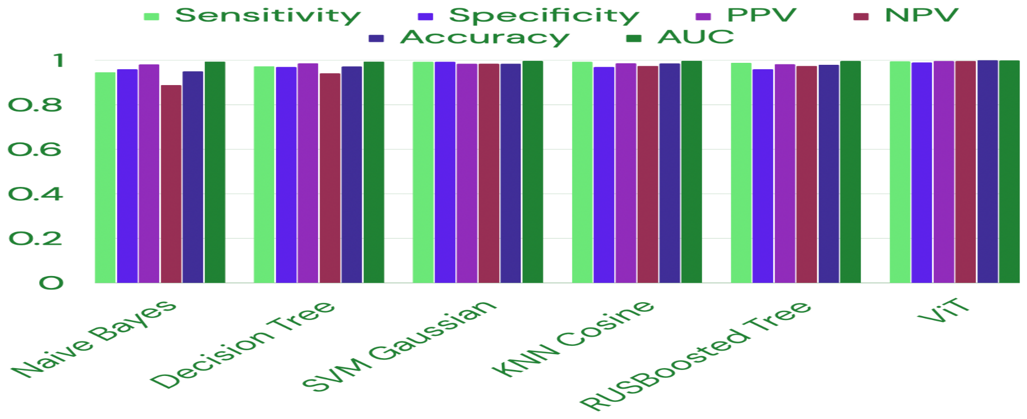

Table 1.
GLCM Features
| Feature | Formula |
|---|---|
| Energy (ASM) | |
| Contrast | |
| Homogeneity | |
| Correlation |
Table 2.
Prostate gland segmentation performance of the proposed method versus the optimized U-Net baseline.
Table 2.
Prostate gland segmentation performance of the proposed method versus the optimized U-Net baseline.
| Method | Dice | IoU | Precision | Recall | ROC_AUC | PR_AUC |
|---|---|---|---|---|---|---|
| Optimized U-Net | 0.831 | 0.705 | 0.872 | 0.784 | 0.9743 | 0.912 |
| Proposed Method | 0.9048 | 0.728 | 0.889 | 0.803 | 0.9870 | 0.928 |
Table 3.
Summary statistics of the proposed segmentation model (mean ± std over the test set). Accuracy, F1 score, and F2 score are reported as pixel level segmentation metrics.
Table 3.
Summary statistics of the proposed segmentation model (mean ± std over the test set). Accuracy, F1 score, and F2 score are reported as pixel level segmentation metrics.
| Metric | Mean | Std |
|---|---|---|
| Dice Similarity Coefficient | 0.904 | 0.0224 |
| Hausdorff Distance (mm) | 2.11 | 0.11 |
| Average Surface Distance (mm) | 3.31 | 0.31 |
| Accuracy | 0.998 | 0.003 |
| F1-Score | 0.844 | 0.018 |
| F2-Score | 0.862 | 0.017 |
Table 4.
Prostate cancer detection performance of the proposed ViT model with adaptive thresholding and morphological opening.
Table 4.
Prostate cancer detection performance of the proposed ViT model with adaptive thresholding and morphological opening.
| Class | Precision | Recall | F1-Score | Support |
|---|---|---|---|---|
| Normal | 0.998 | 0.997 | 0.989 | 66 |
| PCa | 0.998 | 0.987 | 0.987 | 134 |
| Accuracy | 0.998 | 200 | ||
| Macro Avg | 0.989 | 0.988 | 0.990 | 200 |
| Weighted Avg | 0.987 | 0.989 | 0.990 | 200 |
Table 5.
Ablation study showing the incremental effect of each framework component on detection performance.
Table 5.
Ablation study showing the incremental effect of each framework component on detection performance.
| Model Variant | DSC | AUC | Accuracy |
|---|---|---|---|
| Baseline (ViT only) | N/A | 0.850 | 0.820 |
| + Augmentation and preprocessing | N/A | 0.880 | 0.860 |
| + Segmentation guidance | 0.900 | 0.900 | 0.880 |
| Full model (proposed) | 0.905 | 0.987 | 0.998 |
Table 6.
Comparison with representative published methods for prostate cancer detection and segmentation on the PROSTATEx dataset.
Table 6.
Comparison with representative published methods for prostate cancer detection and segmentation on the PROSTATEx dataset.
| Author | Year | Methods | Task | Dataset | Key Result |
|---|---|---|---|---|---|
| Sumin & Kim [54] | 2026 | Radiomic features | Classification, Segmentation | ProstateX | AUC = 0.85 |
| Hussain et al. [48] | 2018 | Morphological, SIFT, EFDs | Classification | ProstateX | AUC = 0.99 |
| Jung et al. [49] | 2025 | Radiomics | Detection | ProstateX | AUC = 0.90 |
| Ali et al. [50] | 2025 | Volume segmentation | Segmentation | ProstateX, PROMISE12 | DSC = 0.80 |
| Giganti et al. [51] | 2025 | CAD and DL | Detection | ProstateX | AUC = 0.85 |
| This study | — | (i) GLCM features + ML (ii) 3D ViT + segmentation guidance | Segmentation-guided detection | ProstateX | (i) Acc = 98.1%, AUC = 0.98 (ii) Acc = 99.8%, AUC = 0.987 DSC = 0.905 |
Disclaimer/Publisher’s Note: The statements, opinions and data contained in all publications are solely those of the individual author(s) and contributor(s) and not of MDPI and/or the editor(s). MDPI and/or the editor(s) disclaim responsibility for any injury to people or property resulting from any ideas, methods, instructions or products referred to in the content. |
© 2026 by the authors. Licensee MDPI, Basel, Switzerland. This article is an open access article distributed under the terms and conditions of the Creative Commons Attribution (CC BY) license (http://creativecommons.org/licenses/by/4.0/).
Copyright: This open access article is published under a Creative Commons CC BY 4.0 license, which permit the free download, distribution, and reuse, provided that the author and preprint are cited in any reuse.