

Submitted:
12 October 2026
Posted:
14 October 2026
You are already at the latest version
Abstract
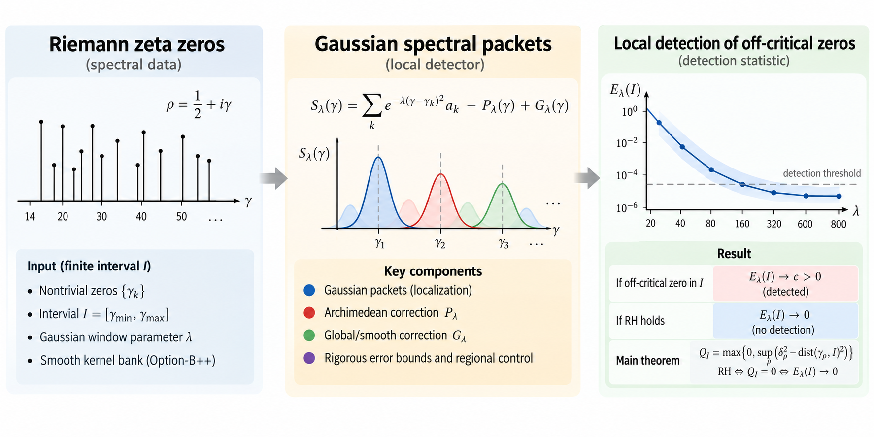
We introduce a Gaussian spectral-packet detector for horizontal displacement of the non-trivial zeros of the Riemann zeta function and connect it quantitatively to the prime side of the explicit formula. For distinct zeros \(\rho=\beta_\rho+i\gamma_\rho\) with multiplicity \(m_\rho\), let \(S_\lambda(t)=\sum_\rho m_\rho e^{-\lambda(z_\rho-t)^2},\qquad z_\rho=\gamma_\rho-i(\beta_\rho-\tfrac12),\) and for a compact interval \(I\), \(Q_I=\max\left\{0,\sup_\rho\left[(\beta_\rho-\tfrac12)^2-\mathrm{dist}(\gamma_\rho,I)^2\right]\right\}\). We prove that the logarithmic exponential rate of \(\sup_{t\in I}|S_\lambda(t)|\) is exactly \(Q_I\): a limsup for arbitrary compact \(I\), and a genuine limit when \(I\) has positive length. The interval lower bound uses an \(O(1/\lambda)\) micro-shift and a finite-dimensional norm-separation argument, preventing dominant-cluster phase cancellation from destroying the exponential rate. This yields an exact RH-equivalent subexponential-growth criterion. Using an even shifted Gaussian and the Guinand–Weil formula in a fixed \(2\pi\) Fourier convention, we derive \(S_\lambda=B_\lambda+G_\lambda-P_\lambda\) and prove an explicit uniform prime-tail estimate. In particular, a finite arithmetic reconstruction preserves the same exponential rate when \(\log N(\lambda)\ge(2+\varepsilon)\lambda\). We then examine the pre-asymptotic regime computationally: finite-prime peak reconstruction, blind synthetic off-critical-pair recovery, multi-pair interference, and nuisance-projected waveform identifiability. These computations test finite-scale identifiability only; they do not prove RH or identify an actual off-critical zero.
Keywords:
Riemann zeta function
; Riemann Hypothesis
; explicit formula
; Gaussian localization
; spectral packets
; prime sums
; computational validation
; identifiability
1. Introduction
The Riemann Hypothesis (RH) asserts that every non-trivial zero of satisfies . The explicit formula connects zeros and primes, but two different questions must be distinguished. The first is mathematical: can one construct a local functional whose exponential rate records horizontal displacement from the critical line even in the presence of interference among zeros? The second is computational: when the corresponding prime-side object is truncated, noisy, projected against nuisance structure, or contaminated by several components, does the predicted signal remain identifiable?
This paper treats both questions in one framework. We use throughout the packet
and, for a compact interval I, the localized exponent
The first half is theorem-driven. A Gaussian packet attached to has the exact factorization
so the natural local exponential exponent is . Theorem 3.10 proves that after summing all zeros and allowing their phases to interfere, the compact-interval logarithmic growth rate is still exactly the geometric envelope . The proof makes precise why a singleton interval gives only a limsup, while a positive-length interval gives a full limit.
The second half asks what survives at finite parameter values. We use two complementary computational models. The arithmetic model reconstructs , detects peaks without feeding the zero ordinates to the detector, and then uses known ordinates only for post-hoc scoring. Controlled synthetic symmetric pairs test blind localization and transverse-rate recovery. The waveform model asks whether a weak second-order defect component survives projection against a local cosine–sine nuisance dictionary. Its main empirical observation is a multi-band collapse in the normalized span , with detectability changing sharply near one local-spacing unit.
The combined architecture is important. The theorem determines what the asymptotic signal means; the explicit formula determines how the signal reaches the prime side; the finite-prime tail theorem specifies which truncations are asymptotically faithful; and the computations show the pre-asymptotic biases and identifiability failures that remain before that regime is reached.
Main Contributions
The paper makes six contributions.
- (C1)
- It proves the exact local exponential detector on positive-length intervals and the corresponding pointwise limsup law.
- (C2)
- It proves non-cancellation by two distinct mechanisms: mean-square recurrence at a point and finite-dimensional norm equivalence after an spatial micro-shift on an interval.
- (C3)
- It gives a normalization-safe Guinand–Weil bridge using an even shifted Gaussian and proves a uniform finite-prime tail estimate.
- (C4)
- It derives an RH-equivalent midrange prime cancellation criterion while explicitly showing that a fixed prime cutoff cannot establish the asymptotic criterion.
- (C5)
- It validates the detector numerically through prime-side peak reconstruction and blind synthetic-pair experiments, including deliberately retained interference failures.
- (C6)
- It identifies an empirical local-spacing resolution law for nuisance-projected waveform detection across five spectral bands and formulates a finite- unknown-component envelope around supplied critical packets.
Remark 1.1
(Claim boundary). No computation in this paper proves or disproves RH. Synthetic defects are sensitivity tests, not observations of unknown zeta zeros. The midrange cancellation statement of Theorem 6.2 is an equivalent reformulation of RH, not an independent proof. Likewise, the finite- packet-residual certificate is conditional on the supplied arithmetic checkpoint, tail bound, and packet model.
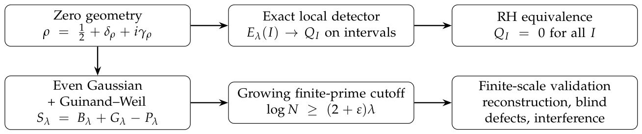
Figure 1.
Logical architecture of the paper. The upper row is the exact zero-side theorem and its RH equivalence. The lower row transports the detector to primes, quantifies the finite-prime approximation, and then studies finite-scale identifiability and failure modes. The computational layer is not used to prove the theorem or RH.
2. Position Relative to Existing Work
The use of explicit formulas to transfer information between primes and zeros is classical, as are RH-equivalent positivity criteria associated with Weil’s quadratic functional [3,7]. Modern variants include Li-type criteria, spectral/operator-theoretic realizations, and screw-function formulations of Weil positivity [8,10,11,14]. These approaches principally encode RH through positivity, quadratic forms, or spectral operators.
Our construction has a different target. It extracts the maximum local horizontal displacement from the exponential rate of a localized Gaussian zero sum. The central issue is therefore not positivity but whether phase interference among several zeros can suppress the leading exponential rate. The pointwise theorem resolves this only in a limsup sense, while the positive-length interval theorem uses an spatial micro-shift to obtain a uniform lower bound for the complete dominant finite cluster. We are not aware of this exact local rate statement, with the outside-interval Gaussian-shadow term and the limsup/limit distinction, in the existing Weil-positivity or operator literature.
There is also recent work on recovering information about zeta zeros from finite or weighted prime data. Balanzario and Cárdenas Romero derive a Hermite-weighted explicit formula and use it to study local zero statistics [12]. Connes obtains high-accuracy critical-line approximants to low zeros by extremizing a finite-prime restriction of Weil’s quadratic form [13], complementing the semilocal prolate-operator program of Connes, Consani and Moscovici [11]. Our finite-prime result is different in form: it gives an explicit growth condition on under which the truncated Gaussian prime packet preserves the same exponential detector rate as the full zero-side packet. The numerical experiments are then used only to study finite- identifiability and failure modes.
For the Guinand–Weil normalization below we use the explicit even-test-function formulation of Chirre and Gonçalves [9], together with the declared -Fourier convention.
3. Gaussian Packets and the Main Theorem
We use the standard zero-counting estimate
and its consequence ; see [4][Ch. 9].
Proposition 3.1
(Local absolute convergence). For every fixed , the series (1) converges absolutely and locally uniformly in t.
Proof.
Let . Since ,
Grouping ordinates into unit shells and using gives a convergent Gaussian majorant. The Weierstrass test proves the claim. □
For fixed t, write
so that
Lemma 3.2
(Attainment of the localized envelope). For every compact interval I,
Hence the supremum in (2) is attained among finitely many zero locations, and .
Proof.
If , then
which tends to . Local finiteness of zeros completes the proof. □
Theorem 3.3
(Spectral upper bound). For every compact interval I,
Proof.
For ,
Fix , with . The finitely many zeros with contribute . For the tail, write . Uniformly for ,
while the number of zeros in the shell is . Hence
Choosing M so that , the tail is for all sufficiently large . Therefore
which proves the assertion. □
3.1. Finite Dominant Clusters
For fixed t, let
Lemma 3.4
(Finite dominant cluster). The set is finite and nonempty. Moreover, there exists such that
Proof.
Since
all near-maximizers lie in a bounded ordinate window, which contains only finitely many zeros. The strict gap follows after removing the finite maximizing set. □
Lemma 3.5
(Exponential-polynomial mean square). Let
where the are distinct and the coefficients are not all zero. Then
and therefore
Proof.
Expand the square. The diagonal terms remain, while every off-diagonal average is bounded by and tends to zero. □
Lemma 3.6
(Pointwise exact exponential rate). For every fixed ,
Proof.
The upper bound follows from Theorem 3.3 applied to the singleton . If , factor
where
After combining equal frequencies, every grouped coefficient is a positive sum of multiplicities, hence is a nonzero finite exponential polynomial. Lemma 3.5 gives an unbounded sequence on which . By the gap in Lemma 3.4, the non-dominant remainder satisfies . Therefore
for all large n. If , nonnegativity of and the upper bound give zero. □
Remark 3.7
(Why only a limsup at one point). A leading exponential polynomial may vanish at arbitrarily large values of ; for example does. Hence a pointwise full limit is not available from dominant-cluster non-cancellation alone.
Lemma 3.8
(Finite-dimensional exponential separation). Let be distinct and let . Then there is a constant , depending only on S and the , such that
for every coefficient vector .
Proof.
The linear map , , is injective because exponentials with distinct exponents are linearly independent on every interval. Restricting T to the unit sphere of the finite-dimensional domain, compactness and continuity imply , which is the stated constant. □
Lemma 3.9
(Uniform micro-shift non-cancellation). Fix , put , and let . Fix and a sign . For
there are constants and such that for ,
where
The lower constant is independent of λ.
Proof.
For , put . Since , direct expansion gives
and
This gives the dominant term exactly. The non-dominant gap at remains positive on an neighborhood, while the Gaussian tail is uniform there; hence the remainder is .
After grouping multiplicities at identical zero locations, the exponents
are distinct. Lemma 3.8, applied with , gives a lower bound whose coefficient -norm is independent of . This proves the uniform lower bound. □
Theorem 3.10
(Exact local Gaussian detection). For every compact interval , possibly a singleton,
If with , then
Consequently,
Proof.
The upper bound is Theorem 3.3. Since
if we may choose a zero attaining the maximum and a nearest point to . Then . Lemma 3.6 gives the limsup lower bound. If , nonnegativity and the upper bound give equality.
Now suppose with . If , the upper bound gives . If , choose as above and a sign pointing into I. There exists a fixed such that for once is large. Lemma 3.9 then yields some with
Hence , and the full limit follows.
If RH holds, every , hence for all I. If RH fails, choose a nondegenerate compact interval containing the ordinate of an off-critical zero; then . This proves (6). □
4. The Gaussian Explicit Formula
We now connect the zero-side detector to primes. Fix the Fourier convention
For and , use the even shifted Gaussian
Its Fourier transform is
The multiset of non-trivial zeros is invariant under , which corresponds to . Absolute convergence therefore gives
Define
Because the gamma-factor integrand is even in u, the archimedean term () is the same as one obtains from a single shifted Gaussian.
Theorem 4.1
(Gaussian explicit formula). With the normalization above,
Moreover, for every compact interval I,
Proof.
Apply the even-test-function Guinand–Weil formula in the -Fourier convention stated above; for a formulation with matching convention and admissibility hypotheses see Proposition 5 of Chirre and Gonçalves [9]. Equation (8) identifies the zero side. Moreover,
and
Thus the pole, prime and gamma-factor terms are exactly , , and . Finally, Stirling’s formula on vertical strips gives
and Gaussian localization yields (13) uniformly on compact t-intervals. □
Remark 4.2
(Normalization discipline). The even test function is used throughout this section. This avoids silently applying an even-test-function explicit formula to a non-even shifted Gaussian. The zero symmetry then recovers the desired one-sided packet sum exactly.
Lemma 4.3
(Exponential-rate stability under subexponential perturbations). Let be bounded functions on a fixed compact interval I, and suppose
Then and have the same limsup logarithmic exponential rate. If the rate of is a genuine limit, the perturbed rate has the same limit.
Proof.
The inequality gives the upper comparison. Interchanging and gives the reverse comparison. After taking logarithms and dividing by , the contribution of vanishes. □
5. Finite-Prime Reconstruction
For , define
and
Proposition 5.1
(Uniform finite-prime tail). Let . If and , then uniformly in ,
Consequently, for every fixed , if
then
Proof.
Using and ,
Set
For ,
Hence the integral test gives
With ,
Completing the square and setting yields
Define the finite arithmetic packet
Corollary 5.2
(Growing-cutoff arithmetic detection). Let satisfy
for some fixed and all sufficiently large λ. Then for every compact interval I,
If I has positive length, the limsup is a genuine limit. Consequently,
for every nondegenerate compact interval I.
Proof.
By (12),
Proposition 5.1 gives a uniformly exponentially small remainder. Lemma 4.3 therefore transfers the exact rate of Theorem 3.10 to . □
Remark 5.3
(Why the cutoff must grow). A fixed prime cutoff is not an RH detector in the limit . The arithmetic reconstruction theorem requires a cutoff growing at least like . Therefore a vanishing rate at fixed N cannot be promoted to a statement about RH.
6. An RH-Equivalent Midrange Prime Criterion
Fix and a function with
Decompose into low, midrange, and high parts according to
Write these pieces as , , and .
Proposition 6.1
(Low and high ranges). Uniformly in t,
and
Proof.
For the low range, discard the Gaussian weight and use :
whose logarithm is . For the high range we apply Proposition 5.1 directly at the real threshold (equivalently one may use ). This avoids any floor-function endpoint ambiguity while preserving the constant . □
Define
Theorem 6.2
(Prime-side reformulation). For every fixed admissible decomposition above,
Proof.
From (12),
On a fixed compact interval the bracketed term has subexponential growth by Theorem 4.1 and Proposition 6.1. Lemma 4.3 transfers the logarithmic exponential rate of to the midrange defect. The conclusion follows from Theorem 3.10. □
Remark 6.3
(No reduction in difficulty). Theorem 6.2 isolates a concrete Gaussian-weighted prime cancellation problem, but it is an equivalence theorem. Proving the stated subexponential cancellation without assuming RH is therefore an RH-level task.
7. Finite-Scale Calibration Model
The exact theorem concerns the true zero packet as . For computational validation we use a controlled symmetric pair as a model perturbation. This section records the elementary calibration law so that the numerical experiments do not depend on an unstated interpretation.
Proposition 7.1
(Symmetric-pair packet). For a model pair , , the combined contribution of the two reflected zeros to the real packet is
At the center,
and therefore on every interval containing ,
Proof.
Insert into the Gaussian packet and add the two conjugate contributions. The displayed formula follows by elementary algebra. The center gives the lower bound. Since the Gaussian envelope is bounded by , the matching upper bound is immediate. □
Proposition 7.2
(Background-separated finite-scale rate). Suppose a background satisfies, at the model center,
for some . Then
Thus the asymptotic rate is unchanged, although finite-λ slope estimates can be biased when the background is not exponentially separated.
Proof.
Factor from the sum at . The residual factor is , and taking the logarithm gives the result. □
Remark 7.3.
The hypothesis of Proposition 7.2 is a model separation condition, not a theorem about the Stage-5 background at the small values . The blind experiments below are precisely intended to measure the pre-asymptotic departure from the idealized separated regime.
8. Computational Models and Experimental Design
8.1. Finite Prime-Side Reconstruction
The arithmetic track uses
where and are the pole and archimedean terms and
The reported Stage-5 run used
with 18,001 grid points and spacing . Peak detection used the arithmetic signal first; known zero ordinates entered only afterward for localization error scoring.
8.2. Synthetic Symmetric Pair
A symmetric model pair with center and horizontal displacement contributes the real packet
The blind Stage-6B estimator sees only over the search interval; the injected labels are withheld until post-fit scoring.
For each , the largest absolute response is quadratically refined to give . The primary finite-scale growth estimate is the least-squares slope
The clipping is used only when reporting ; the raw signed is retained for diagnostics. A separate fit of
against is recorded as an asymptotic-facing diagnostic.
8.3. Waveform Identifiability Model
The second experimental track uses the first 1600 positive zero ordinates and a local carrier block. The clean local waveform is
where the phases are reproducibly perturbed with standard deviation . A synthetic defect residual at center c is proportional to
with . Its amplitude is rescaled to have RMS equal to of the clean waveform RMS, and independent Gaussian observation noise of RMS is then added.
The nuisance matrix contains both cosine and sine carriers for the K local frequencies. If is its singular-value decomposition, the hard projector retains singular vectors satisfying
The raw second-order defect template is
and the residualized template is
Its survival fraction
measures how much defect geometry remains outside the local nuisance space. The detection score is the normalized correlation of the observed waveform with the unit-normalized residualized template. ROC AUC is used to compare defect and clean scores; AUC represents chance-level ranking [16].
8.4. Local-Spacing Scaling Variable
For an observation span L and a local spacing estimate g, define
Five disjoint 320-zero bands were studied. The band-median gaps and corresponding values are shown in Table 1.
The tested nominal values were
with the physical span L adjusted separately in each band. Each condition used 256 admissible centers and five noise seeds, producing 6400 clean/defect score pairs per pooled band-median bin.
9. Experimental Protocol
9.1. Arithmetic Reconstruction and Blind Recovery
Stage 5 computed the prime-side background up to , including 1,270,607 primes and 732 prime-power terms with exponent at least two. At each of the five values, ten peaks were detected in . Stage 6 added visible synthetic defects for calibration. Stage 6B then withheld the pair parameters from the estimator and performed blind recovery at two centers:
for . The first center lies on a strong reconstructed critical packet; the second lies between nearby known zeros. A two-pair experiment with separation was used as an interference stress test.
9.2. Waveform Train/Validation/Test Organization
The 1600 ordinates were partitioned by index into train , validation , and test regions. The later local-spacing study pooled five spectral bands only after the detector design and threshold had been fixed. The use of disjoint spectral ranges was intended to prevent direct reuse of identical carrier neighborhoods across train, validation, and test stages.
Earlier V3.9 and V4.0 experiments established that short observation windows can allow the nuisance space to absorb most of the defect template. The later V4.3–V4.5 program therefore tested whether span should be normalized by a local zero-spacing scale rather than treated as an absolute length.
9.3. Finite-Lambda Unknown-Component Certificate
The V4.31–V4.32 certification stage separates the finite arithmetic signal from a packet field built from supplied critical-line ordinates. If
and is a certified pointwise prime-tail bound, then
An optional common ordinate uncertainty adds the conservative budget
where M is the number of supplied positive ordinates. Equation (21) is a finite- certificate around the supplied packet model, not an asymptotic proof of RH.
10. Computational Results
10.1. Prime-Side Reconstruction Localizes the First Ten Peaks
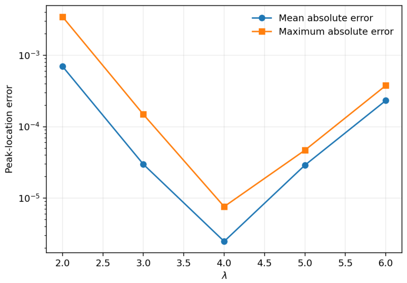
All five Stage-5 rows returned ten detected peaks before zero ordinates were used for scoring. The finite-cutoff localization error is smallest near the middle of the tested range; Table 2 summarizes the reported values.
Figure 2 shows the same finite-cutoff behavior on a logarithmic error scale. The non-monotonicity with is a useful warning: increasing localization strength without increasing the prime cutoff does not guarantee uniformly improved reconstruction.
Figure 2.
Finite-cutoff peak localization error versus . The best localization in this run occurs at , not at the largest .
Figure 2.
Finite-cutoff peak localization error versus . The best localization in this run occurs at , not at the largest .
10.2. Blind Single-Pair Recovery Exposes Background-Dependent Bias
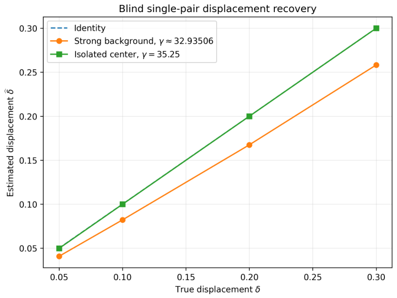
Table 3 compares blind displacement estimates at the two injected centers. At , the log-slope estimator is nearly unbiased over the tested range. At the strong reconstructed critical packet near , the same estimator underestimates every injected displacement.
The corresponding localization estimates are also accurate: the median recovered center differs from by only a few in the single-pair tests, and recovery at is at the sub-micro level in the reported runs. Thus the main finite-scale difficulty is not finding the center but estimating the transverse growth rate in the presence of structured background.
Figure 3.
Blind displacement recovery. The between-zero injection at tracks the identity line closely; injection on top of the reconstructed critical packet near shows systematic downward bias.
Figure 3.
Blind displacement recovery. The between-zero injection at tracks the identity line closely; injection on top of the reconstructed critical packet near shows systematic downward bias.
10.3. Two-Pair Interference Breaks the Naive Global Estimator
The two-pair stress test is deliberately adversarial. The raw log-slope estimates are
for true , respectively. Because three fitted rates are negative, clipping q before taking a square root would report in those cases. Even at true , the clipped estimate is only .
Figure 4.
Failure of the naive global growth-rate estimator under two-pair interference. Negative fitted rates must be retained as diagnostics rather than silently clipped into a “no defect” conclusion.
Figure 4.
Failure of the naive global growth-rate estimator under two-pair interference. Negative fitted rates must be retained as diagnostics rather than silently clipped into a “no defect” conclusion.
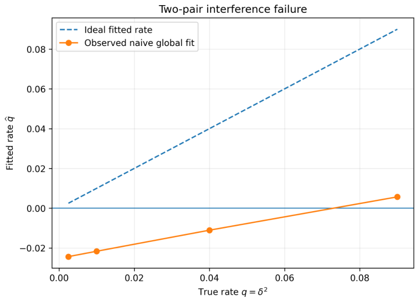
This experiment demonstrates that a blind global supremum statistic is not a reliable multi-defect estimator at finite . Interference is therefore not a small numerical nuisance; it changes the qualitative behavior of the fitted growth rate.
10.4. A Local-Spacing Transition Controls Waveform Identifiability
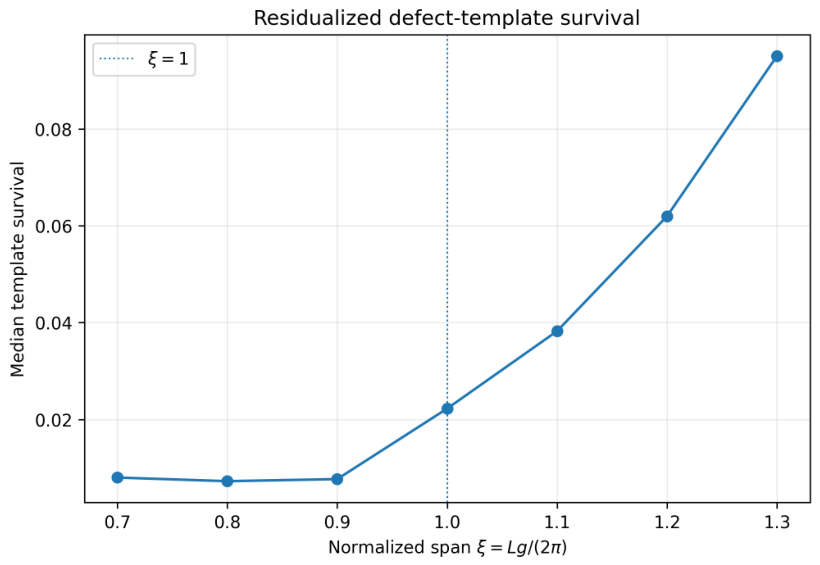
The V4.4 multi-band experiment produces the clearest scale law in the computational program. Using band-median spacing, the residualized-template survival remains of order below , then grows rapidly. The pooled ROC AUC exhibits the same transition (Table 4).
Figure 5.
Pooled ROC AUC versus normalized span for the band-median spacing definition. The empirical transition is concentrated near .
Figure 5.
Pooled ROC AUC versus normalized span for the band-median spacing definition. The empirical transition is concentrated near .
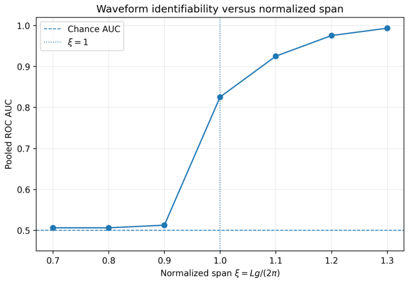
Figure 6.
Median residualized-template survival versus normalized span. Increased survival of the defect template outside the nuisance subspace accompanies the AUC transition.
Figure 6.
Median residualized-template survival versus normalized span. Increased survival of the defect template outside the nuisance subspace accompanies the AUC transition.
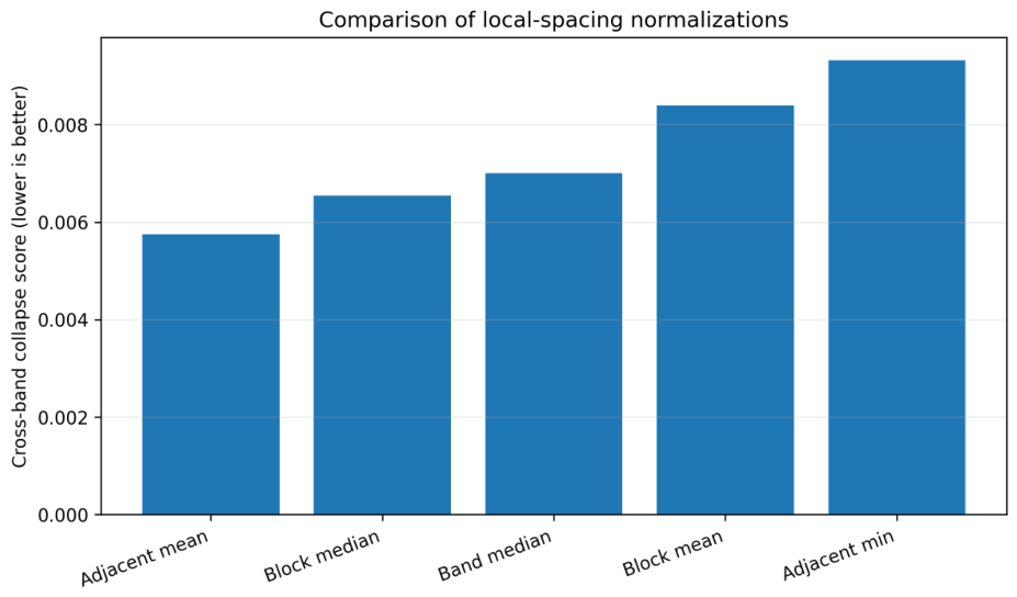
The collapse is not tied to one particular spacing definition. Five definitions were compared by cross-band dispersion. Lower is better:
Thus adjacent-mean spacing provides the best collapse among the tested normalizations, while the band median gives a simple transparent summary of the transition.
Figure 7.
Cross-band collapse scores for five spacing normalizations. Adjacent-mean spacing is best among the tested definitions.
Figure 7.
Cross-band collapse scores for five spacing normalizations. Adjacent-mean spacing is best among the tested definitions.
11. Interpretation of the Finite-Scale Experiments
11.1. The Critical Scale Is a Resolution Scale, Not an RH Threshold
Equation (20) suggests that the effective observation span should be measured relative to a local spectral spacing. Empirically, leaves the second-order defect template almost contained in the local carrier space, while exposes a detectable orthogonal component. The sharpness of the AUC transition across five height bands supports a local-resolution interpretation.
This does not mean that is a universal theorem or an RH threshold. It is an empirical critical scale for this particular nuisance model, template, phase distribution, noise level, and local dictionary. The best-performing spacing definition is also center-local rather than global.
11.2. Background Overlap Explains Finite- Bias
The contrast between injections at and shows that finite- rate recovery depends strongly on local background geometry. Near a strong critical packet, the total amplitude is not a pure law and the fitted slope underestimates q. Away from such a packet, the same estimator is nearly exact over the tested values.
This behavior is consistent with the finite- separation picture in Section 7 and with the exact detector of Section 3, Section 4 and Section 5: the asymptotic rate can be correct while the finite-window estimator carries an exponentially decaying background correction. The numerical results therefore argue for debiasing or explicit background projection rather than for changing the asymptotic detector itself.
11.3. Interference Is a Structural Identifiability Failure
The two-pair experiment is more serious than the single-background bias. Here the blind global statistic can decrease with , producing negative fitted q despite positive injected defects. Any operational detector must therefore preserve signed diagnostic rates, localize candidate components, and avoid interpreting clipping to zero as evidence of absence.
The waveform experiments reach the same conclusion from a different direction: if the nuisance space is too flexible relative to the observation span, the defect template is absorbed before classification. Successful detection requires not only signal amplitude but also geometric separation from the nuisance model.
11.4. Finite-Lambda Unknown-Component Envelopes
The V4.31–V4.32 residual program formalizes a useful finite-height question: after subtracting supplied critical-line packets, how large can the remaining infinite detector be once the finite-prime tail is added? The pointwise envelope (21) is valuable because it separates three contributions: finite arithmetic residual, certified prime tail, and optional zero-ordinate uncertainty.
Its interpretation is deliberately limited. If the zero cache is not itself supplied with rigorous ordinate and critical-line certificates, attribution of the residual to “known critical packets” remains diagnostic. Even with certified ordinates, a small finite- envelope is not an asymptotic proof of RH.
12. Theory–Experiment Crosswalk
The combined paper is intentionally organized so that each numerical experiment answers a finite-scale question generated by a specific theorem or obstruction. Table 5 records that relation and prevents empirical output from being used outside its justified scope.
13. Limitations and Claim Discipline
The theorem layer and computational layer have different logical strengths, and the following boundaries are part of the result rather than disclaimers added after the fact.
- (1)
- Synthetic defects. Off-critical pairs are engineered perturbations. No experiment identifies an actual off-critical zeta zero.
- (2)
- Fixed prime cutoff. Stage 5 uses , whereas Corollary 5.2 requires asymptotically. Fixed-N behavior cannot prove RH.
- (3)
- Finite . Blind fits use ; background overlap and interference can dominate the asymptotic rate at such scales.
- (4)
- Multiple components. The global maximum-based estimator is demonstrably unstable under two nearby synthetic pairs.
- (5)
- Waveform model dependence. The -transition is measured for a fixed nuisance dictionary, phase distribution, residual RMS, noise level, and . It is not a theorem about zeta zeros.
- (6)
- Zero cache. The 1600 ordinates used in the waveform study are external numerical inputs. Proof-grade attribution would require independent certification of ordinates and critical-line status.
- (7)
- Finite-lambda certificate. The V4.32 envelope is rigorous only relative to the supplied finite arithmetic checkpoint, tail certificate, packet model, and ordinate-error assumption.
- (8)
- Open analytic step. The midrange prime cancellation criterion is exactly RH-equivalent. The present work isolates but does not solve it.
14. Reproducibility and Supporting Ledger
The accompanying archive contains the manuscript, all six figures and compact CSV tables used in the computational sections, the Stage-5/6/6B source pipeline and transcript, waveform scripts V3.9–V4.5, the V4.31/V4.32 residual/certificate scripts, a zero-cache regeneration helper, and a separate detailed proof-and-evidence ledger. The ledger records the dependency chain for every theorem and the data lineage for every headline numerical value.
The historical heavy computations are not silently regenerated with altered code. Where a result is preserved in a transcript or frozen CSV, the manuscript reports that archived value. Randomized waveform experiments use deterministic seeds in the scripts. The principal V4.4 parameters are
The archived V4.5 script requires the historical raw V4.4 center-condition table, which is not frozen in the present archive, so we do not claim a center-level V4.5 rerun. No pooled V4.4 observation is treated as iid for uncertainty quantification; a future clustered bootstrap should resample at the center/band level after the raw center-condition table is frozen.
15. Open Problems
Open Problem 15.1 (Unconditional midrange cancellation) For one fixed decomposition of Section 6, prove
for every nondegenerate compact interval I, without assuming RH. By Theorem 6.2, this is equivalent to RH.
Open Problem 15.2 (Finite-scale multi-component inference) Construct a localized estimator whose finite- output remains stable under several nearby symmetric pairs and prove a quantitative separation/interference theorem.
Open Problem 15.3 (Resolution law) Determine whether the empirical scale can be derived from a precise singular-value or uncertainty principle for the local carrier dictionary, and identify the dependence on K, phase perturbation, and noise.
Open Problem 15.4 (Certified large-parameter reconstruction) Develop interval- or ball-arithmetic implementations of with simultaneously certified prime-tail, quadrature, grid, and rounding errors at larger and growing N.
16. Acknowledgements
AI Disclosure:In the preparation of this manuscript, the author utilized a custom-built, open-source generative AI language model to assist with structural brainstorming, LaTeX formatting, and proofreading. The author directed all prompts, independently verified all mathematical derivations and logical arguments, and takes full responsibility for the accuracy and originality of the final text.
17. Conclusion
Gaussian spectral packets provide an exact local exponential detector for horizontal displacement of zeta zeros. The zero-side theorem is robust to phase interference at the exponential scale, and an even-Gaussian Guinand–Weil formula transports the detector to the prime side. A growing finite-prime cutoff retains the same rate, while the remaining midrange cancellation criterion is precisely RH-equivalent.
The computational results clarify how this exact asymptotic picture degrades at finite scale. Prime-side peak localization can be highly accurate at an intermediate smoothing parameter, isolated synthetic defects can be recovered almost exactly, and strong critical backgrounds create systematic rate bias without destroying center localization. Nearby components can defeat a naive global slope through destructive interference. Independently, nuisance-projected waveform experiments show that defect identifiability changes sharply when the observation span reaches roughly one local-spacing unit.
The combined theory and computation therefore identify both the signal and the obstruction. The signal is the exponential rate ; the obstructions are central-prime cancellation, finite cutoff, overlap, nuisance geometry, and interference. None of the finite experiments proves RH, but together they provide a mathematically anchored and reproducibly stress-tested framework for studying what a local off-critical signature would have to look like.
Data and code availability
All scripts, compact data tables, archived transcripts, figures, and the supporting proof/evidence ledger used to generate the reported results are included in the accompanying reproducibility package. Numerical zero ordinates are external inputs; for independent comparison we cite Odlyzko’s tabulation [15].
Conflicts of Interest
The author declares no conflict of interest.
References
- Edwards, H. M. Riemann’s Zeta Function; Academic Press, 1974. [Google Scholar]
- Guinand, A. P. A summation formula in the theory of prime numbers. Proc. Lond. Math. Soc. (2) 1948, 50, 107–119. [Google Scholar] [CrossRef]
- Weil, A. Sur les “formules explicites” de la théorie des nombres premiers. Comm. Sém. Math. Univ. Lund. 1952, 252–265. [Google Scholar]
- Titchmarsh, E. C.; Heath-Brown, D. R. (Eds.) The Theory of the Riemann Zeta-Function, 2nd ed.; Oxford University Press, 1986. [Google Scholar]
- Iwaniec, H.; Kowalski, E. Analytic Number Theory. In AMS Colloquium Publications; 2004; p. 53. [Google Scholar]
- Montgomery, H. L. The pair correlation of zeros of the zeta function, in Analytic Number Theory. Proc. Symp. Pure Math. 1973, 24, 181–193. [Google Scholar]
- Bombieri, E. Remarks on Weil’s quadratic functional in the theory of prime numbers, I. In Atti Accad. Naz. Lincei Rend. Lincei Mat. Appl.; 2000; Volume 11, pp. 183–233. [Google Scholar]
- Bombieri, E.; Lagarias, J. C. Complements to Li’s criterion for the Riemann hypothesis. J. Number Theory 1999, 77, 274–287. [Google Scholar] [CrossRef]
- Chirre, A.; Gonçalves, F. Bounding the log-derivative of the zeta-function. Math. Z. 2022, 300, 1041–1053. [Google Scholar] [CrossRef]
- Suzuki, M. Aspects of the screw function corresponding to the Riemann zeta-function. J. Lond. Math. Soc. 2023, 108, 1448–1487. [Google Scholar] [CrossRef]
- Connes, A.; Consani, C.; Moscovici, H. Zeta zeros and prolate wave operators: semilocal adelic operators. Ann. Funct. Anal. 2024, 15, 87. [Google Scholar] [CrossRef]
- Balanzario, E. P.; Cárdenas Romero, D. E. An explicit formula for the zeros of the Riemann zeta function and the statistics of their local distribution. Ramanujan J. 2026, 69, 21. [Google Scholar] [CrossRef]
- A. Connes, The Riemann Hypothesis: past, present and a letter through time. J. Open Math. Probl. 2026, arXiv:2602.040222(1), 1–52.
- Suzuki, M. Weil’s quadratic form via the screw function. arXiv 2026, arXiv:2606.09096. [Google Scholar]
- Odlyzko, A. M. Tables of zeros of the Riemann zeta function. [CrossRef]
- Fawcett, T. An introduction to ROC analysis. Pattern Recognit. Lett. 2006, 27, 861–874. [Google Scholar] [CrossRef]

Table 1.
Spectral bands used in the span-collapse experiment.
| Band | Zero indices | Median gap g | |
|---|---|---|---|
| 0 | 0–319 | 1.609522 | 3.904 |
| 1 | 320–639 | 1.259728 | 4.988 |
| 2 | 640–959 | 1.148644 | 5.470 |
| 3 | 960–1279 | 1.097626 | 5.724 |
| 4 | 1280–1599 | 1.048560 | 5.992 |
Table 2.
Stage-5 peak localization error after post-hoc matching to the first ten positive zeta-zero ordinates in .
Table 2.
Stage-5 peak localization error after post-hoc matching to the first ten positive zeta-zero ordinates in .
| Mean absolute error | Maximum absolute error | |
|---|---|---|
| 2 | ||
| 3 | ||
| 4 | ||
| 5 | ||
| 6 |
Table 3.
Blind Stage-6B single-pair recovery. Injected parameters are used only for post-fit scoring.
Table 3.
Blind Stage-6B single-pair recovery. Injected parameters are used only for post-fit scoring.
| True | at | at |
|---|---|---|
| 0.05 | 0.040752 | 0.049744 |
| 0.10 | 0.082121 | 0.099877 |
| 0.20 | 0.167440 | 0.199948 |
| 0.30 | 0.258221 | 0.299973 |
Table 4.
Pooled band-median V4.4 results. Each row contains 6400 paired score observations across five spectral bands.
Table 4.
Pooled band-median V4.4 results. Each row contains 6400 paired score observations across five spectral bands.
| Template survival | Pooled AUC | Paired win rate | |
|---|---|---|---|
| 0.70 | 0.5061 | 0.7477 | |
| 0.80 | 0.5061 | 0.7569 | |
| 0.90 | 0.5125 | 0.7858 | |
| 1.00 | 0.8254 | 0.9428 | |
| 1.10 | 0.9251 | 0.9775 | |
| 1.20 | 0.9755 | 0.9981 | |
| 1.30 | 0.9934 | 1.0000 |
Table 5.
Crosswalk between exact statements and finite-scale experiments.
| Theory object | Computational test | Valid interpretation |
|---|---|---|
| Theorem 3.10: rate | Hidden single symmetric pair | Checks whether finite- localization/rate fitting approaches the model exponent; does not test an unknown zero. |
| Theorem 4.1: | Stage-5 prime-side peak reconstruction | Checks implementation/localization of the arithmetic packet at one fixed cutoff. |
| Corollary 5.2: growing cutoff | Fixed scan | Illustrates finite behavior only; the theorem explicitly forbids promoting fixed-N convergence to RH. |
| Proposition 7.2 | Strong-background versus isolated-center injections | Quantifies pre-asymptotic bias caused by overlap; near-unbiased isolated recovery is consistent with separation. |
| Dominant-cluster interference | Two-pair stress test | Demonstrates that a naive global slope can fail under finite-scale cancellation. |
| Local spectral geometry | Nuisance-projection waveform experiment | Measures whether the defect template survives the local carrier space; is empirical/model-dependent. |
| Exact packet plus certified tail | V4.31–V4.32 residual envelope | Produces a finite-, model-relative upper envelope; not an asymptotic theorem about all zeros. |
| Theorem 6.2: RH-equivalent cancellation | No finite experiment closes it | The central analytic cancellation remains open; no AUC or finite scan substitutes for it. |
Disclaimer/Publisher’s Note: The statements, opinions and data contained in all publications are solely those of the individual author(s) and contributor(s) and not of MDPI and/or the editor(s). MDPI and/or the editor(s) disclaim responsibility for any injury to people or property resulting from any ideas, methods, instructions or products referred to in the content. |
© 2026 by the authors. Licensee MDPI, Basel, Switzerland. This article is an open access article distributed under the terms and conditions of the Creative Commons Attribution (CC BY) license (http://creativecommons.org/licenses/by/4.0/).
Copyright: This open access article is published under a Creative Commons CC BY 4.0 license, which permit the free download, distribution, and reuse, provided that the author and preprint are cited in any reuse.