

Submitted:
13 October 2026
Posted:
14 October 2026
You are already at the latest version
Abstract
A researcher who backtests many trading strategies and keeps the best one faces two questions: how much to believe the winner's backtest, and whether searching more candidates leads to a better strategy. We show that, when strategies are sampled at random from a fixed pool, the second question has an exact answer: the expected out-of-sample payoff at any search width is a known weighted average of the leaderboard, the out-of-sample payoff of each in-sample rank. We measure that leaderboard for 652 mechanical trading signals on U.S. mega-cap stocks (2010-2025) and on industry and size/value portfolios (1970-2025), trading one day after the signal and paying realistic spreads. Three results stand out. The backtest always overstates, and the overstatement grows with search width. Net of costs, searching more candidates picks a less costly strategy, mainly slow momentum, so the chosen strategy improves relative to a narrow search on the diversified panels. But at no width does any rule, including shrinkage and combination, find a strategy with a reliably positive return after costs.
Keywords:
backtest overfitting
; strategy selection
; search width
; transaction costs
; empirical Bayes
; out-of-sample evaluation
1. Introduction
Machine learning is now applied to financial data at every scale, down to individual transactions [17], and automated research tools generate and backtest thousands of trading strategies in an afternoon. That makes one design choice newly important: how many candidates to search before picking one. Searching more has an obvious cost: the best of many backtests is more likely to be lucky, so its reported performance is more inflated. It may also have a benefit: a wider search is more likely to contain a genuinely good strategy. Which effect dominates for the strategy you actually hold?
The literature has mostly studied the first effect, how far to discount a winning backtest [1,8]. We study both effects and keep them separate. We call the winner’s backtested performance the report and the strategy actually held the choice. The report can be badly wrong while the choice is fine, and the reverse; a single statistic cannot settle both.
What we do.
We make one object the center of the analysis: the backtest leaderboard, the average out-of-sample return of the strategy ranked j-th in-sample, for every rank j. Section 3 shows that under random-subset search, the expected out-of-sample payoff of the most common selection rules, at every search width, is an exact weighted average of this leaderboard with known hypergeometric weights. Wider search simply puts more weight on the top ranks. So the practical question “should I search more?” becomes “does the top of the leaderboard beat the ranks just below it?” We then measure the leaderboard on three U.S. panels, with a one-day trading delay and measured bid–ask costs.
What we find.
- 1.
- The report is always inflated, and more so with wider search (Figure 2). On mega-caps the winner of a 256-strategy search reports a net return of bp a year in its backtest and earns out of sample.
- 2.
- Net of costs, wider search improves the choice on diversified panels, but only relative to a narrow search (Figure 3). Selecting on net backtest performance, going from 16 to 256 candidates raises the winner’s out-of-sample return by bp a year on industry portfolios and on size/value portfolios, mostly by finding strategies that trade less. On mega-caps the gain is indistinguishable from zero for the single winner and positive for a top-4 portfolio.
- 3.
- No width finds a strategy worth holding. Under our main cost model the best net return across widths, panels and eight selection, shrinkage and combination rules is bp a year, with a confidence interval that includes zero (Figure 5). Under the lower and upper cost models, the exact width curves never exceed bp a year.
Contributions.
(i) An exact reduction from search width to the shape of the leaderboard, with a simple corollary: if out-of-sample payoffs never improve as you move down the in-sample ranking, searching more can never hurt the single winner. (ii) Width varied as a controlled treatment, with selection rule and portfolio size held fixed, on real trading strategies graded out of sample net of measured costs. (iii) A benchmark of selection against shrinkage and combination under the same cost accounting, with trades netted across strategies.
2. How This Relates to Past Work
Discounting the winner.
Grading the choice.
A smaller literature asks whether the selected strategy is good. The probability of backtest overfitting [2] measures how often the in-sample winner falls below the out-of-sample median; it summarizes where the in-sample winner lands on our leaderboard. Chen [3] apply empirical Bayes to about 136,000 mined long–short strategies and find that naively mining for the largest Sharpe ratios performs similarly, while only empirical Bayes delivers unbiased predictions of performance. That is close to a report/choice split, and our shrinkage results agree with it. The decision-theory version of the split is the optimizer’s curse [7,14]. What we add is search width as the treatment and costs as part of the outcome.
Costs and implementation.
Anomaly returns shrink sharply after trading costs [13] and after publication [12]. We build costs bottom-up from quoted spreads and from the effective-cost estimates of Hasbrouck [9], cross-checked against the century of large-stock spreads in Jones [10]. Daily portfolio returns are known to contain stale-price autocorrelation [11], which is why we trade one day late.
Best-of-n in machine learning.
Language-model alignment studies the same trade-off: as more candidates are scored by an imperfect reward model, the true reward of the selected output can rise and then fall [5]. Finance offers an unusually clean test bed: the “gold” reward is future returns, observed only after the selection is frozen.
3. Method
3.1. Setup: Report, Choice and Leaderboard
There are N candidate strategies. In each evaluation period (an epoch) we rank them by in-sample Sharpe ratio over the previous three years (rank 1 is best) and record each rank’s out-of-sample mean return over the next six months. Let be the out-of-sample return of the rank-j strategy in epoch e. The leaderboard is , shown beside its in-sample counterpart. A researcher with width n sees only a random subset of n candidates and applies a selection rule: pick-best holds the subset’s top strategy; top-k holds its top k in equal weights. The report is the selected strategy’s in-sample return; the choice is its out-of-sample return.
3.2. The Exact Reduction
Proposition
(Width is a weighting of the leaderboard). Under uniform random n-subsets of N ranked candidates, the probability that rank j is the pick-best winner is
and the expected weight on rank j in an equal-weight top-k portfolio () is
Hence the expected out-of-sample payoff at width n is for pick-best and for top-k. The expected report is the same weighting applied to the in-sample leaderboard.
Corollary 1.
rises with n. So if is non-increasing in j, the pick-best payoff never falls as width grows. Width can hurt the choice only if the top of the leaderboard underperforms ranks below it.
Proofs are in Appendix Section 7. Mean return is linear in portfolio weights, so these curves are exact and free of the subset-sampling noise of Monte Carlo designs. An independent script verifies them by brute-force simulation and by full enumeration, and checks numerically that the top-k curves are also monotone under a non-increasing leaderboard. At , a width-16 search finds the global best strategy 2.5% of the time and has a median winner rank of 28; a width-256 search finds it 39% of the time with a median winner rank of 2.
3.3. Data and Candidate Strategies
- Mega-caps: the 1,000 CRSP stocks with the largest average market capitalization among those with at least 3,500 trading days (funds excluded), 2010–2025 (out-of-sample 2013–2025; 25 epochs).
- Industries: the 49 value-weighted Fama–French industry portfolios, 1970–2025 (out-of-sample 1973–2025; 106 epochs).
- Size/value: the 25 value-weighted size and book-to-market portfolios, same dates.
The candidate set is 652 mechanical cross-sectional signals with no hand-picking: moving-average crossovers (trend), past-return momentum with several lookbacks and skips, and short-term reversal, each in both directions and some volatility-scaled. Each signal becomes a daily dollar-neutral long–short portfolio with $1 of gross exposure.
3.4. Trading Delay and Costs
A signal formed at Monday’s close is traded at Tuesday’s close and earns Wednesday’s return (a one-day delay). Turnover is measured with positions drifting with returns between trades. Each dollar traded pays a half-spread:
- Mega-caps: each stock’s closing quoted half-spread (median 1.5 bp).
- Portfolios: the value-weighted half-spread of the stocks in the same size quintile. Sources are Hasbrouck’s effective-cost estimates (1970–1992), his trade-level sample (1993–2005) and CRSP quotes (2010–2025), interpolated for 2006–2009 (Appendix Section 8). The value-weighted average falls from about 33 bp in the 1970s to about 2 bp after 2010.
Strategies are selected on in-sample net Sharpe ratio, so the researcher knows about costs. We also report a lower and an upper cost model (Appendix Section 8).
3.5. Inference and Evidence Discipline
Confidence intervals resample blocks of six consecutive epochs, because adjacent in-sample windows overlap. That leaves 18 independent blocks on the portfolio panels and only 5 on mega-caps. The test of whether the top of the leaderboard beats the next tier permutes rank labels within the top 50 inside each epoch, which uses every epoch. All samples in this paper are discovery data that earlier versions of this study had already examined. A one-time test on never-examined pre-2010 single-stock data is preregistered (Section 6), and every analysis is logged with the number of times its sample had been examined (Appendix Section 9).
4. Findings
4.1. The Leaderboard
Figure 1 is the paper in one picture. In every panel the in-sample curve (gray) sits well above the out-of-sample curve (blue): the backtest overstates at every rank. Before costs, out-of-sample returns are positive and roughly flat across the top 100 ranks of the industry and size/value panels, which means the ranking carries information but the top ranks are not much better than rank 50. After costs (orange), returns are at or below zero even at the very top and fall steeply below it: because the ranking is on net performance, the lower ranks collect the strategies whose trading costs exceed their gross return.
4.2. Report Versus Choice as Search Widens
Figure 2 applies Proposition 1 to both curves of Figure 1. The report (purple) rises steadily with width on every panel: searching more always makes the winner’s backtest look better. The choice (orange) rises much less, and on mega-caps not at all beyond a few dozen candidates. The gap between them, the overstatement, grows with width on mega-caps and industries and levels off beyond a few hundred candidates on size/value. On mega-caps the winner of a 256-strategy search reports bp a year net of costs and earns (Table 1). This is the familiar winner’s curse, now measured net of costs and as a function of width.
4.3. What Wider Search Buys
Searching more improves the net choice on both portfolio panels (Table 1): bp a year on industries and on size/value, going from 16 to 256 candidates, with confidence intervals well above zero. Figure 3 shows why. On the portfolio panels, a wider search finds strategies that trade less (the gray cost line falls by half) while earning more before costs. Slow momentum signals fill about 90% of the top ten. On mega-caps, the two effects cancel: the strategies a wide search finds trade less but also earn less, so the single winner’s net return is flat. Top-4 portfolios gain from width on all three panels.
The improvement is relative. Even at the best width, the winner’s out-of-sample net return is bp a year on industries, on size/value and on mega-caps. Wider search picks a less bad strategy.
Corollary 1 says width can only hurt if the top of the leaderboard underperforms the next tier. Before costs, that happens on industries: ranks 1–5 earn 96 bp a year less than ranks 6–50 (), and the pick-best curve peaks near 32 candidates. After costs the sign flips, because the top net ranks are the strategies that trade least, and that advantage persists out of sample.
4.4. The One-Day Delay
Like many daily backtests, earlier versions of this study traded each signal at the same close that produced it. Figure 4(a) shows what a one-day delay does. On industry portfolios, the best 10% of the old backtest earned 805 bp a year out of sample with next-day trading, with a one-day delay and with two. Panel (b) explains the pattern. The next-day profit is largest from the 1960s to the 1990s, when portfolios’ own day-to-day autocorrelation exceeds their cross-autocorrelation. That own autocorrelation is strongest in small-stock portfolios (0.44 for the smallest size quintile of the size/value panel versus 0.24 for the largest, in the 1970s), turns negative after 2000, and the profit disappears with a one-day delay. That is the signature of stale prices in portfolio returns, not a tradable effect. Mega-cap signals, by contrast, survive the delay. Short-term reversal earns about the same with quote midpoints as with closing prices, so it is not bid–ask bounce; with 41% daily turnover it roughly breaks even at the quoted spreads of these stocks.
4.5. Selection Versus Shrinkage and Combination
Figure 5 compares eight rules at full width on all three panels, with trades netted across strategies. Holding the top four instead of the top one helps on both portfolio panels (by 180 and 165 bp a year) and makes no difference on mega-caps (). Ranking by empirical-Bayes posterior mean rather than raw Sharpe changes little: on size/value it picks the same four strategies, and elsewhere it adds 38–74 bp a year with intervals that include zero [consistent with [3]. Weighting by the posterior mean mostly holds cash. On mega-caps it holds cash in every epoch, because no strategy’s shrunk Sharpe ratio is positive. That is the right answer when nothing has a positive expected net return. Naive combinations do worst. A ridge mean-variance blend and equal weights across all 652 strategies lose hundreds of basis points a year on mega-caps and thousands on the portfolio panels, because blending hundreds of fast signals produces a portfolio that trades 35–42% of its book every day. The best rule anywhere earns bp a year (EB top-4 on industries, Sharpe ratio 0.19). The best on mega-caps is an equal-weight top 16 at . Both intervals include zero.
5. Conclusion
The backtest leaderboard turns “how many strategies should I search?” into a question that data can answer: does the top of the in-sample ranking beat the ranks just below it, after costs? On three U.S. panels, three practical rules follow.
- 1.
- Always discount the report. Once more than a few candidates are searched, the winner’s backtest overstates its out-of-sample return on every panel, before and after costs, and by more as the search widens.
- 2.
- Select on net-of-cost performance, and hold a few strategies rather than one. Selecting on net performance is what makes wider search help. With trades netted, the top four beat the single winner by 165–180 bp a year on both portfolio panels and match it on mega-caps.
- 3.
- Do not expect width to manufacture alpha. Wider search finds the least costly of a set of signals; it does not turn a set with no net edge into one with an edge.
6. Limitations and Next Steps
Limitations.
All samples here are discovery data that earlier versions of this study had already examined, so every number above is provisional. Mega-caps give only five independent blocks, and their universe is chosen on full-sample size and history, which tilts it toward survivors. The exact width curves charge each strategy its own costs, which overstates costs for top-k portfolios relative to the netted portfolios of Section 4.5. Commissions are not modeled. Jones [10] estimates that spreads and commissions together cost at least 1% of dollar volume from 1953 to 1975, so our early net returns are optimistic. Random-subset search is a model of width, not of how researchers actually search; sequential, adaptive search is a natural extension.
Next steps.
- 1.
- One sealed test. A preregistered amendment fixes the primary test (top 5 versus ranks 6–50, net of quoted spreads, one-day delay) for a single run on never-examined 1993–2009 single-stock data, and for a forward run on 2026–2028 data after mid-2028.
- 2.
- The risk report. Earlier work found that selecting the lowest-estimated-risk portfolio understates realized risk by more as width grows. That result must be retested against a null that keeps real volatility clustering, and after standard eigenvalue corrections, before it returns to the main text.
- 3.
- Mechanism. Test whether the flat top of the gross leaderboard is explained by light-tailed true skill plus estimation noise, using the empirical-Bayes prior estimated here.
A Proofs
Proposition 1.
A uniform random n-subset contains rank j as its best member exactly when it contains j and its other members come from the worse ranks: of the equally likely subsets. For top-k, rank j is in the subset with probability ; given that, the number of better ranks among the other members is hypergeometric with population , successes and draws, and j is held (with weight ) when that number is at most . The expected payoff is linear in these weights. The same argument applied to in-sample returns gives the expected report.
Corollary 1.
The winner has rank greater than k exactly when all n members come from the ranks below k, which has probability , decreasing in n. So the winner’s rank at width is first-order stochastically smaller than at width n. If is non-increasing, is non-decreasing in n. The independent verification script also confirms the analogous monotonicity for top-k () on 2,000 random non-increasing leaderboards each, with no violations.
B. Cost Model
Mega-caps.
Each stock-day’s half-spread is at the close, kept when ; missing days take the median of the stock’s previous 21 quotes. Coverage is 99.8%; the median is 1.5 bp. The upper model doubles it. A low-frequency high–low estimator proved unusable for these stocks: its yearly median swings between 0 and 22 bp with market volatility.
Portfolios.
For each year and NYSE size quintile we take the value-weighted half-spread of member stocks. The 49 industries use the all-stock average, because the sources carry no industry codes.
- 1970–1992: Hasbrouck’s Gibbs estimates of effective cost [9].
- 1993–2005: his trade-level comparison sample.
- 2010–2025: CRSP closing quotes.
- 2006–2009: log-linear interpolation.
Against the trade-level data, the Gibbs estimates are accurate for the smallest quintile but overstate the largest by 2–7 times after the mid-1990s, when spreads became too small for daily data to resolve. Before 1993 we keep them unscaled, because Dow stocks’ quoted spreads were near 0.6% (about 30 bp half-spread) in the 1950s and 1980s [10], at or above the Gibbs values for the largest quintile. The lower model scales pre-1993 values by each quintile’s 1993–1995 ratio of trade-level to Gibbs cost (0.48 for the largest). The upper model keeps Gibbs through 2005 and doubles quoted spreads after 2010. Conclusions are the same under all three models.
C. Evidence Accounting
Every analysis is logged with its date, its sample, the sample’s status (discovery, previously used holdout, or never examined) and how often that sample had been examined before. The industry panel had been examined in about twenty earlier analyses, so every result on it is exploratory rather than confirmatory. Two holdouts from earlier work, French 1927–1969 and 1,000 never-examined CRSP names, were each opened once before the cost and delay layers existed. In both, the winner’s reported optimism stayed within a pure-selection benchmark. Those runs used next-day trading before costs; we now read them as evidence about the report, not the choice. Pre-2010 single stocks and the 2026–2028 future remain sealed.
References
- Bailey, D.H.; López de Prado, M. The deflated Sharpe ratio: correcting for selection bias, backtest overfitting and non-normality. J. Portf. Manag. 2014, 40(5), 94–107. [Google Scholar] [CrossRef]
- Bailey, D.H.; Borwein, J.M.; López de Prado, M.; Zhu, Q.J. The probability of backtest overfitting. J. Comput. Financ. 2017, 20(4), 39–69. [Google Scholar] [CrossRef]
- Chen, A.Y.; Dim, C. 2025, High-throughput asset pricing, working paper. arXiv, (version 3); arXiv:2311.10685.
- Chordia, T.; Goyal, A.; Saretto, A. Anomalies and false rejections. Rev. Financ. Stud. 2020, 33(5), 2134–2179. [Google Scholar] [CrossRef]
- Gao, L.; Schulman, J.; Hilton, J. Scaling laws for reward model overoptimization. In Proceedings of the 40th International Conference on Machine Learning, 2023; pp. 10835–10866. [Google Scholar]
- Hansen, P.R. A test for superior predictive ability. J. Bus. Econ. Stat. 2005, 23(4), 365–380. [Google Scholar] [CrossRef]
- Harrison, J.R.; March, J.G. Decision making and postdecision surprises. Adm. Sci. Q. 1984, 29(1), 26–42. [Google Scholar] [CrossRef]
- Harvey, C.R.; Liu, Y.; Zhu, H. and the cross-section of expected returns. Rev. Financ. Stud. 2016, 29(1), 5–68. [Google Scholar] [CrossRef]
- Hasbrouck, J. Trading costs and returns for U.S. equities: estimating effective costs from daily data. J. Financ. 2009, 64(3), 1445–1477. [Google Scholar] [CrossRef]
- Jones, C.M. A century of stock market liquidity and trading costs, working paper; Columbia University, 2002. [Google Scholar]
- Lo, A.W.; MacKinlay, A.C. When are contrarian profits due to stock market overreaction? Rev. Financ. Stud. 1990, 3(2), 175–205. [Google Scholar] [CrossRef]
- McLean, R.D.; Pontiff, J. Does academic research destroy stock return predictability? J. Financ. 2016, 71(1), 5–32. [Google Scholar] [CrossRef]
- Novy-Marx, R.; Velikov, M. A taxonomy of anomalies and their trading costs. Rev. Financ. Stud. 2016, 29(1), 104–147. [Google Scholar] [CrossRef]
- Smith, J.E.; Winkler, R.L. The optimizer’s curse: skepticism and postdecision surprise in decision analysis. Manag. Sci. 2006, 52(3), 311–322. [Google Scholar] [CrossRef]
- Sullivan, R.; Timmermann, A.; White, H. Data-snooping, technical trading rule performance, and the bootstrap. J. Financ. 1999, 54(5), 1647–1691. [Google Scholar] [CrossRef]
- White, H. A reality check for data snooping. Econometrica 2000, 68(5), 1097–1126. [Google Scholar] [CrossRef]
- Xu, Z.; Xia, J.; Yi, Y.; Chang, M.; Liu, Z. Discrimination of financial fraud in transaction data via improved Mamba-based sequence modeling. In Proceedings of the 2025 International Symposium on Machine Learning and Social Computing (MLSC ’25), New York, 2025; Association for Computing Machinery; pp. 519–524. [Google Scholar] [CrossRef]
Figure 1.
The backtest leaderboard. Mean annual return of the strategy at each in-sample rank (log scale), averaged over epochs and smoothed across neighboring ranks; bands are 90% block-bootstrap intervals. Gray: the in-sample backtest. Blue: out of sample before costs. Orange: out of sample after costs, with selection on net Sharpe. All with a one-day trading delay.
Figure 1.
The backtest leaderboard. Mean annual return of the strategy at each in-sample rank (log scale), averaged over epochs and smoothed across neighboring ranks; bands are 90% block-bootstrap intervals. Gray: the in-sample backtest. Blue: out of sample before costs. Orange: out of sample after costs, with selection on net Sharpe. All with a one-day trading delay.
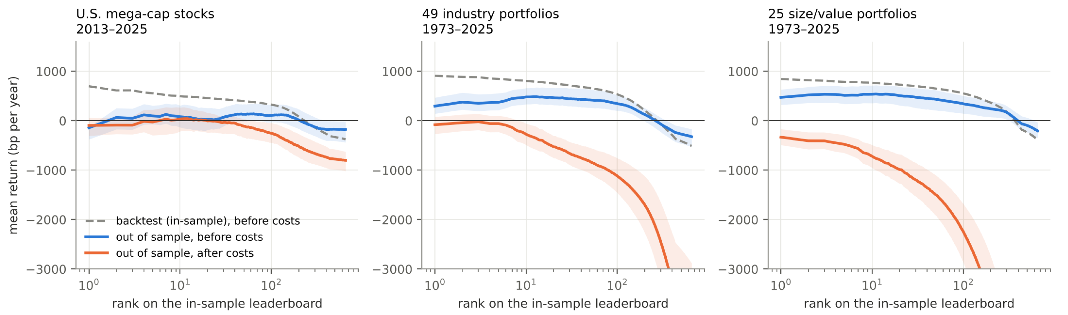
Figure 2.
What the backtest reports versus what you get. For the pick-best winner of a random n-strategy search, selected on net Sharpe: its in-sample net return (purple) and its out-of-sample net return (orange), from the exact weights of Proposition 1. The shaded gap is the overstatement.
Figure 2.
What the backtest reports versus what you get. For the pick-best winner of a random n-strategy search, selected on net Sharpe: its in-sample net return (purple) and its out-of-sample net return (orange), from the exact weights of Proposition 1. The shaded gap is the overstatement.
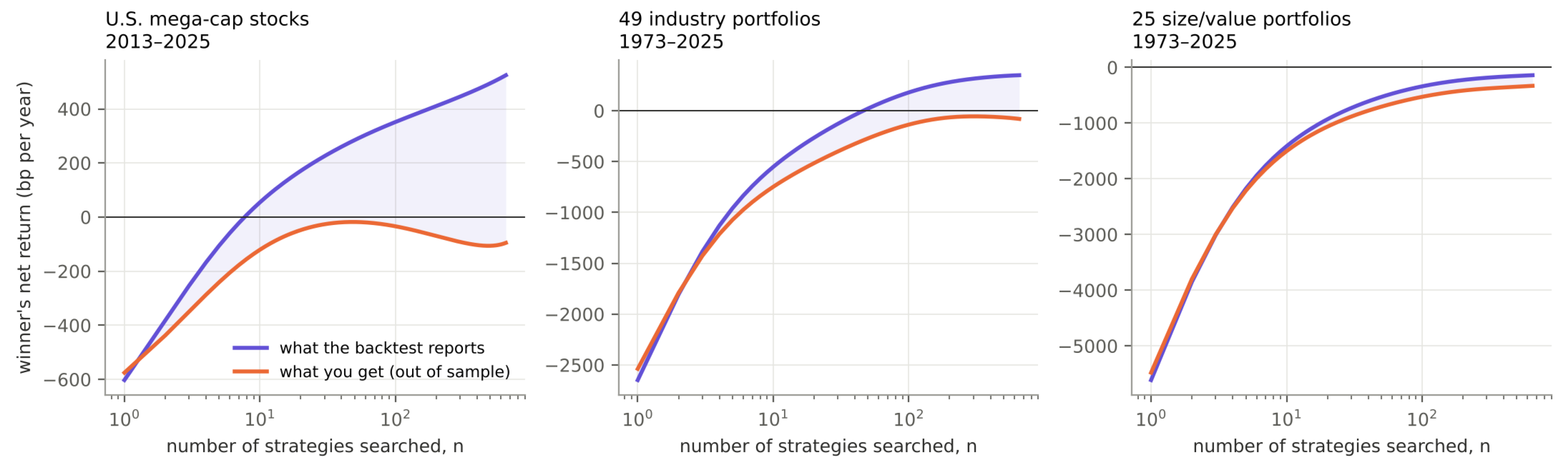
Figure 3.
Where the improvement comes from. For the pick-best winner selected on net Sharpe: out-of-sample return before costs (blue), trading cost (gray) and net return (orange), by search width. Exact weights; one-day delay; main cost model.
Figure 3.
Where the improvement comes from. For the pick-best winner selected on net Sharpe: out-of-sample return before costs (blue), trading cost (gray) and net return (orange), by search width. Exact weights; one-day delay; main cost model.
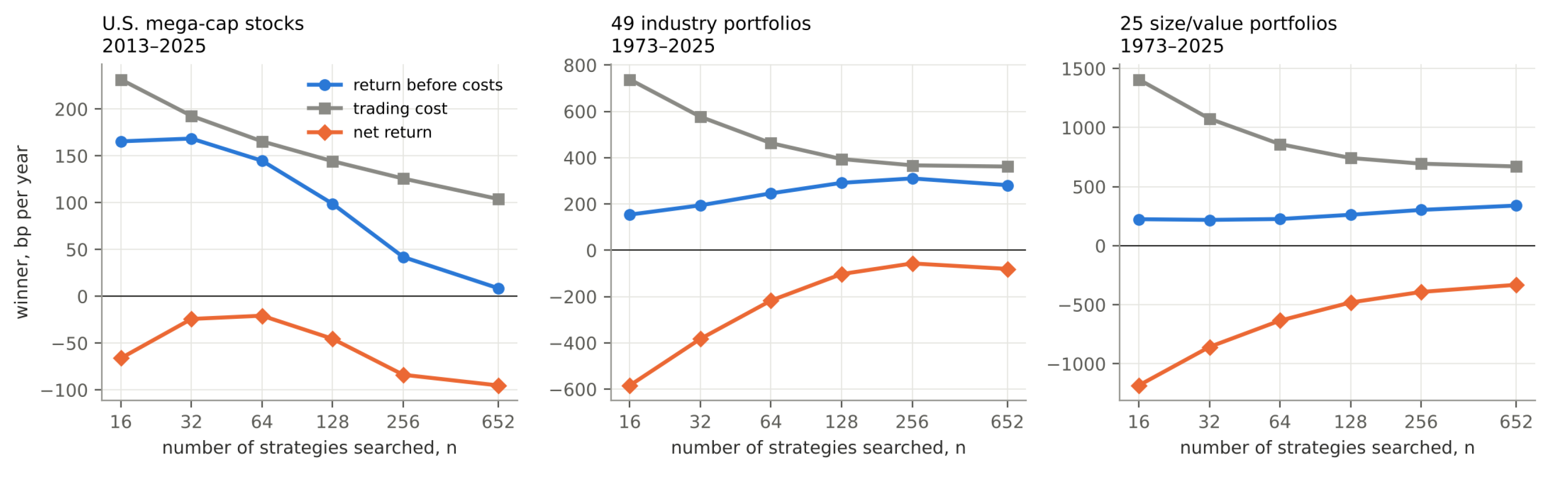
Figure 4.
Trading one day late. (a) Out-of-sample return, before costs, of the top 10% of strategies on the original next-day backtest, when the same signals are traded one, two or three days after formation. (b) Expected profit of a relative-strength strategy on industry portfolios [11] with next-day trading and with a one-day delay, by decade. The shaded decades served as a holdout sample in earlier work.
Figure 4.
Trading one day late. (a) Out-of-sample return, before costs, of the top 10% of strategies on the original next-day backtest, when the same signals are traded one, two or three days after formation. (b) Expected profit of a relative-strength strategy on industry portfolios [11] with next-day trading and with a one-day delay, by decade. The shaded decades served as a holdout sample in earlier work.
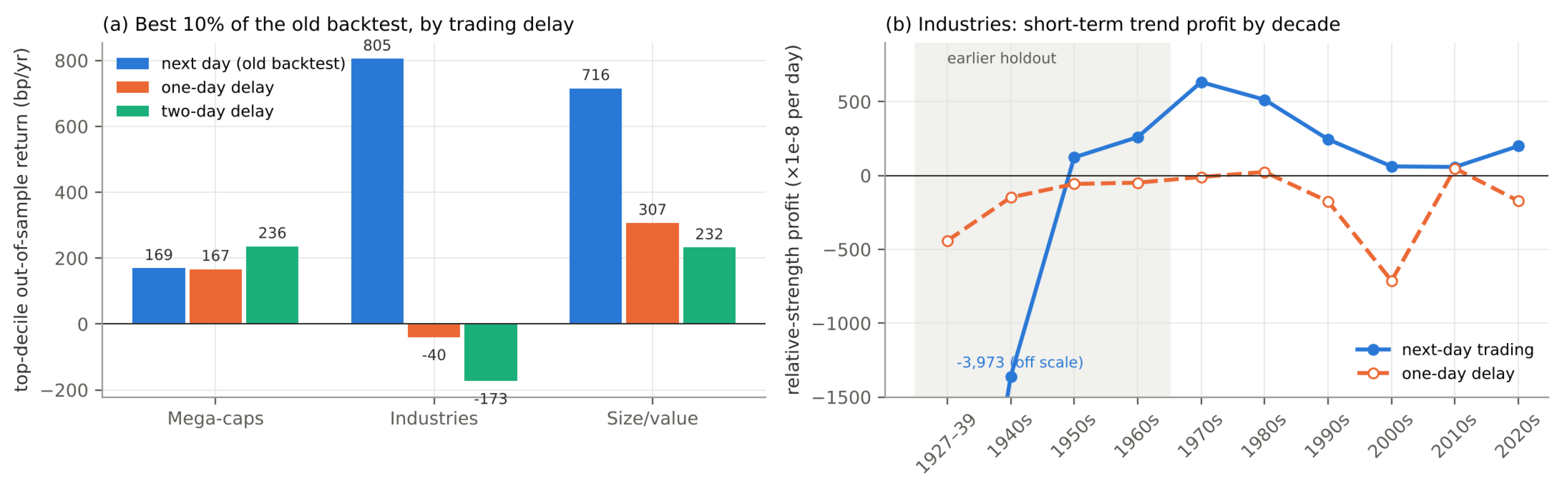
Figure 5.
Is anything worth holding? Out-of-sample net return with 95% block-bootstrap intervals for eight rules applied to all 652 strategies. Costs are charged on the combined portfolio, so trades that cancel across strategies are free. EB: empirical-Bayes posterior mean of the Sharpe ratio. Off-scale points are printed.
Figure 5.
Is anything worth holding? Out-of-sample net return with 95% block-bootstrap intervals for eight rules applied to all 652 strategies. Costs are charged on the combined portfolio, so trades that cancel across strategies are free. EB: empirical-Bayes posterior mean of the Sharpe ratio. Off-scale points are printed.
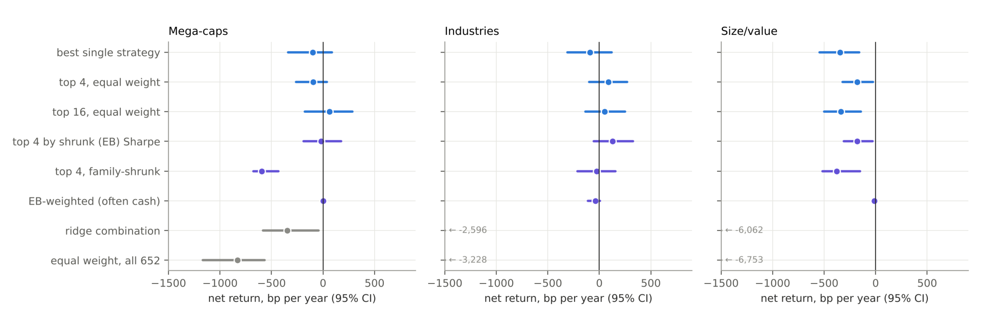

Table 1.
Headline numbers. One-day delay; main cost model; selection on net in-sample Sharpe (the before-costs row ranks on gross). p-values from within-epoch permutation of rank labels in the top 50.
Table 1.
Headline numbers. One-day delay; main cost model; selection on net in-sample Sharpe (the before-costs row ranks on gross). p-values from within-epoch permutation of rank labels in the top 50.
| Mega-caps | Industries | Size/value | |
|---|---|---|---|
| Pick-best winner at , net of costs (bp/yr) | |||
| Backtest (report) | |||
| Out of sample (choice) | |||
| Gain from searching 256 rather than 16 strategies (bp/yr, 95% CI) | |||
| Pick-best | |||
| Top-4 | |||
| Does the top beat the next tier? Ranks 1–5 minus 6–50 (bp/yr) | |||
| Before costs | () | () | () |
| After costs | () | () | () |
| Independent blocks | 5 | 18 | 18 |
Disclaimer/Publisher’s Note: The statements, opinions and data contained in all publications are solely those of the individual author(s) and contributor(s) and not of MDPI and/or the editor(s). MDPI and/or the editor(s) disclaim responsibility for any injury to people or property resulting from any ideas, methods, instructions or products referred to in the content. |
© 2026 by the authors. Licensee MDPI, Basel, Switzerland. This article is an open access article distributed under the terms and conditions of the Creative Commons Attribution (CC BY) license (http://creativecommons.org/licenses/by/4.0/).
Copyright: This open access article is published under a Creative Commons CC BY 4.0 license, which permit the free download, distribution, and reuse, provided that the author and preprint are cited in any reuse.