

Submitted:
12 October 2026
Posted:
13 October 2026
You are already at the latest version
Abstract
Population health research in Canada frequently assigns environmental and area-based exposures to individuals using residential postal codes. Of the several tools available for this process, the most common is the Postal Code Conversion File Plus (PCCF+), which uses population-weighted random allocation for postal codes with multiple potential geographic locations. However, the positional error of this method, and its consequences for assignment of environmental exposures or area-based deprivation, have not been comprehensively measured against a national address register. This study geocoded 12.4 million residential addresses from the National Address Register (NAR) with PCCF+ Version 8D and compared each assigned PCCF+ representative point with a reference location given by the NAR building point or, where that was absent, a matched Open Database of Addresses point or the NAR blockface point. Positional error, dissemination area (DA) agreement, growing-season greenness from the MODIS Enhanced Vegetation Index (EVI), and quintiles of the Material and Social Deprivation Index were compared across postal delivery modes and categories of rurality. The median error was 65 m for urban addresses served by letter carriers and 3.1 km for rural postal codes, and DA agreement was 92% and 30%, respectively. Greenness assigned from PCCF+ was nearly unbiased for urban houses (mean absolute difference 0.013) but was systematically higher than at the true location for rural postal codes (bias +0.036; r = 0.51). The material deprivation quintile was misclassified for 5.0% of urban addresses and 46.2% of rural postal-code addresses, with errors distributed symmetrically. Misclassification depended far more on delivery mode than on rurality: rural postal codes were misclassified at similar rates (about 44% to 49%) in metropolitan areas, census agglomerations and most metropolitan influenced zones, and less often in areas with no metropolitan influence. Error measures and two correction methods were developed from the register: a stratum correction based on the probability of each assigned deprivation quintile given the true quintile, by province, Statistical Area Classification (SAC) and delivery mode, and, for record-level data, a postal-code correction based on the distribution of true quintiles within each postal code. Delivery mode explained about twice as much of the error as province and SAC combined, and error measures stratified only by province and SAC misstated misclassification by 20 to 40 percentage points for populations with atypical delivery-mode mixes. In simulated cohorts with a true rate ratio of 2.0, naive estimates were attenuated by 5% nationally and by up to 31% in rural Saskatchewan, whereas the postal-code correction reduced bias to under 3% with 92–100% interval coverage across all cohort types. Exposure misclassification from postal code geocoding is concentrated among rural addresses and attenuated deprivation gradients in simulated cohorts, and it can be corrected using national address data.
Keywords:
geocoding
; postal codes
; positional error
; exposure misclassification
; misclassification correction
; greenness
; area-based deprivation
; rural health
; National Address Register
; Canada
1. Introduction
In epidemiologic research, residential location links individuals to the environmental and social conditions that shape health, and for most studies in Canada that link is made through the postal code. Administrative health records, cohort studies and linked census files commonly retain the six-character residential postal code but not the full civic address. Researchers must therefore first convert postal codes to geographic coordinates or census geographic areas and then attach exposures measured at those locations, such as surrounding greenness or Census-derived social deprivation [1,2,3,4]. This conversion is indirect, because postal codes, environmental exposures and census areas differ in scale and form, and each difference can introduce error. The accuracy of the conversion method therefore affects the accuracy of every exposure assigned through it.
A postal code is a mail delivery construct rather than a location. Urban postal codes served by letter carriers typically correspond to one side of a street block or a single apartment building, whereas rural postal codes may serve a post office and the surrounding territory over many kilometres, and post office boxes and general delivery are tied to postal installations rather than to dwellings [5,6]. Statistics Canada distributes the Postal Code Conversion File Plus (PCCF+) to manage this ambiguity: where a postal code links to several areas, PCCF+ allocates each record among the candidate dissemination areas (DAs) in proportion to their population, and it reports the delivery mode type (DMT) and the precision of the representative point assigned [6].
Previous Canadian evaluations have shown that the accuracy of postal code geocoding depends on delivery mode and settlement size. Bow and colleagues reported that urban postal code coordinates were a reasonable proxy for residential location in Calgary [7]. Khan and colleagues compared PCCF+ coordinates with street-address locations for a sample of 1,004 census respondents and found median errors of 0.16 to 0.33 km in communities of at least 10,000 people but 5.6 km in rural areas, with delivery mode as the principal determinant of accuracy [8]. Terashima and Kephart, using the Nova Scotia Civic Address File, found that DA and census subdivision (CSD) misclassification was more frequent in rural than in urban areas [9], and Pinault and colleagues found that residents with rural postal codes were matched to a single DA only 13.9% of the time, compared with 87.1% for residents of the urban core of a census metropolitan area or agglomeration [10]. These studies document the postal code geocoding problem but are limited to small samples, single provinces, or the census geography of the postal code itself, and none quantified how positional error is transferred into assigned exposure values.
Exposure misclassification is rarely neutral in its consequences [11]. Nondifferential error in a continuous exposure generally attenuates exposure-response associations, while error that differs between population groups can distort comparisons between them [2,12]. If postal code geocoding misclassifies greenness or deprivation mainly for rural residents, studies of urban-rural health inequities may underestimate gradients among rural populations or misattribute differences between and within settings.
The release of the National Address Register (NAR) by Statistics Canada allows postal code geocoding to be validated nationally and methods to be developed that quantify and correct its error. The NAR provides georeferenced civic addresses for the whole country, with a building location for most addresses and a mailing postal code for each [13]. This study used the NAR as a reference standard to address four objectives: (1) to quantify the positional error of PCCF+ geocoding and its variation by delivery mode and rurality; (2) to measure the resulting misclassification of greenness and area-based deprivation; (3) to model these differences as a function of delivery mode and rurality, in order to determine whether misclassification is differential across the rural-urban gradient; and (4) to develop and validate methods that correct deprivation-based estimates for postal code geocoding error, stratified by province, rurality and delivery mode, with an explicit error term and interval estimates.
2. Materials and Methods
2.1. Study Design and Data Sources
This cross-sectional validation study compared, for each residential address in Canada, a reference location derived from address registers with the representative point assigned by PCCF+ using the address's postal code. Several sources were combined (Table 1 lists sample counts). The NAR (June 2026 release) provided civic addresses, building use, mailing postal codes, building points and blockface representative points [13]. The Open Database of Addresses (ODA, version 1), a compilation of municipal and provincial open address points, supplied an alternative reference location [14]. PCCF+ Version 8D (December 2025 postal codes, 2021 census geography) was the geocoding system under evaluation [6]. Greenness was measured with the MODIS Terra vegetation index product MOD13Q1 Version 6.1 [15,16], and area-based deprivation with the 2021 Material and Social Deprivation Index (MSDI) of the Institut national de santé publique du Québec [4,17]. Rurality was classified with the 2021 Statistical Area Classification (SAC) assigned through the 2021 Geographic Attribute File (GAF), and the Index of Remoteness was attached at the CSD level for descriptive analyses [18,19,20]. All spatial operations used the Statistics Canada Lambert projection (EPSG:3347) and the 2021 DA cartographic boundary file.
2.2. Residential Addresses and Reference Locations
All NAR address records were read for the ten provinces and three territories (17,362,476 records). Addresses whose building use was coded as residential were retained (12,740,837), and those without a valid six-character mailing postal code were excluded (42,103 removed). Addresses coded as partially residential were excluded from the main analysis because this category is dominated by mixed-use and multi-unit buildings in large urban centres.
The reference location for each address was assigned by a hierarchy. The NAR building point was used where available (11,678,351 addresses; 92.3%). Where it was absent, the address was matched to the ODA on civic number, standardized street name, street type and direction, accepting a candidate in the same CSD or within 1 km of the NAR blockface point; this supplied 250,264 reference locations (2.0%). The remaining addresses were assigned the NAR blockface representative point (718,890; 5.7%), and 51,229 addresses with none of the three locations were excluded. Addresses without a building point were concentrated in rural and cottage areas, notably in Ontario and Saskatchewan, so the hierarchy was adopted to avoid under-representing the settings in which geocoding error was expected to be largest. Where an address had both a building point and an alternative point, the alternatives were compared with the building point to describe their accuracy (Table S1).
2.3. Geocoding with PCCF+
Each address's postal code was processed through the residential routine of PCCF+ Version 8D in R, with a fixed random seed for each processing batch so that the population-weighted allocation of multi-link postal codes was reproducible. Two changes were made to one helper function of the R implementation without altering the distributed program files: the lookup of candidate links was restructured for speed, which produced output identical to the unmodified program in a test province, and groups in which every allocation weight was zero or missing, which caused the unmodified program to stop, were allocated with equal probability. This fallback applied to 1,826 addresses (0.01%). PCCF+ assigned a point and DA to 12,644,482 addresses (99.98%).
2.4. Delivery Mode and Rurality
Delivery mode was taken from the PCCF+ DMT and grouped as urban letter carrier to a house (DMT A) or apartment building (B), business building or large volume receiver (E, G), rural postal code (W), rural route or suburban service (H, T), post office box, general delivery or other (J, K, M, R, X), and unknown or retired (Z without a prior DMT). For the error measures and correction methods (Section 2.8), these were further grouped as urban letter carrier (DMT A, B, E, G), rural (W, H, T) and other. Rurality was defined by the SAC type of the DA containing the reference location and grouped as census metropolitan area (CMA), census agglomeration (CA), strong, moderate, weak and no metropolitan influenced zone (MIZ), and territories outside a CA [19].
2.5. Exposure Assignment
Greenness was measured with the Enhanced Vegetation Index (EVI), which is less prone to saturation over dense vegetation than the Normalized Difference Vegetation Index [16]. For each 231.7 m MODIS cell, the growing-season value was the mean of the 16-day composites beginning between 1 June and 31 August, retaining observations whose quality flags indicated a valid index without mixed clouds, possible snow or ice, or possible shadow. Values were computed for 2025 and 2026 and averaged. EVI was extracted at the reference location and at the PCCF+ point for the containing cell and for the mean of 3 × 3 (approximately 700 m) and 5 × 5 (approximately 1.2 km) windows; the 3 × 3 window was the primary measure. EVI was unavailable for 11,118 addresses in the main sample (0.09%): 1,627 whose reference location or PCCF+ point lay beyond the northern edge of the MODIS extract (64.4°N), and 9,491 for which the 3 × 3 window had no valid growing-season observation at one of the two points because of cloud, snow or shadow flags or open water. Deprivation was assigned by identifying the 2021 DA containing the reference point and attaching that DA's national MSDI material and social scores and quintiles, and by attaching the same values for the DA assigned by PCCF+ [17].
2.6. Outcomes
Positional error for address i was the geodesic (haversine) distance between the reference location, with latitude φiR and longitude θiR, and the PCCF+ point (φiP, θiP):
where R = 6,371,008.8 m is the mean radius of the Earth. Area agreement was the proportion of addresses for which the PCCF+ DA equalled the DA of the reference location,
and was computed in the same way for CSDs. For greenness, the difference between EVI at the PCCF+ point and at the reference location was summarized as the mean (bias), the mean absolute difference (MAE), the root mean square difference and the Pearson correlation. For deprivation, let n(t, a) be the number of addresses whose reference DA lies in quintile t and whose PCCF+ DA lies in quintile a. Misclassification was any disagreement (t ≠ a), summarized as the misclassification rate, its direction, the proportion of errors of two or more quintiles, and linearly weighted kappa,
with
where n(t, ·) and n(·, a) are the row and column totals.
2.7. Statistical Analysis
Outcomes were described by delivery mode, rurality, their combination, province (Table S7) and address-weighted decile of the CSD-level Index of Remoteness (Table S8). Four regression models were fitted with delivery mode, rurality and their interaction, adjusted for province: ordinary least squares models for the logarithm of positional error and for the absolute EVI difference, and logistic models for material and social quintile misclassification. As all predictors were categorical, each model was estimated from cell-level statistics. Combinations of delivery mode and rurality with fewer than 100 addresses were not modelled. The interaction was tested with an F test or likelihood ratio test, and adjusted predictions were standardized to the provincial distribution of the analytic sample. Given the size of the sample, interpretation focused on effect sizes rather than statistical significance.
The main analytic sample excluded urban letter-carrier addresses (DMT A, B, E and G) whose reference location was the NAR blockface point (232,182 addresses), as PCCF+ also places most urban postal codes on blockface representative points, which would make that comparison partly circular. Sensitivity analyses repeated the descriptive analyses by reference source (building, ODA and blockface), restricted the models to addresses with a building reference point, and compared greenness windows and years.
2.8. Correcting Deprivation Estimates for Geocoding Error
2.8.1. Strata and Error Measures
A study that uses only postal codes will assign each person the DA identifier chosen by PCCF+, so its estimates by deprivation quintile inherit the misclassification described above. Two correction methods were developed from PCCF+ outputs, one for aggregate counts and one for record-level data.
Strata s were defined by the province, the SAC type and the delivery mode of the PCCF+ assignment, with delivery mode grouped as urban letter carrier, rural or other (167 strata). The assigned SAC type agreed with the SAC type of the reference location for 98.6% of addresses. Two coarser stratifications, province × SAC type (64 strata) and province × delivery mode (36 strata), were also evaluated, and the choice among them is described in Section 2.8.5.
For each stratum, the validation data give the counts ns(t, a) defined in Section 2.6, from which the stratum-specific misclassification rate and weighted kappa (Equations (3) and (4)) were calculated as error measures. As the inputs are counts of addresses by reference DA and PCCF+ DA, the same quantities can be derived for any DA-level index, such as the Canadian Marginalization Index [21] or Census summary data, by attaching its DA values.
2.8.2. Stratum Correction for Aggregate Data
The classification probabilities Ps(a | t) are the probabilities that an address in true quintile t is assigned quintile a. These were given a Dirichlet posterior that shrinks small strata toward the national matrix Pg(a | t) for the same SAC type and delivery mode, with prior weight k = 20 addresses per row. Because addresses that share a postal code share its geocoding error, address counts carry less information than independent observations. The design effect ds(t) of this clustering was therefore estimated with a Bayesian bootstrap over postal codes [22], as the ratio of the bootstrap variance of Ps(a | t) to its variance under independent addresses, and the posterior was
with mean
so that the design effect widens the posterior without changing its mean.
Conditioning on the true quintile, rather than on the assigned quintile, means that these probabilities do not depend on the distribution of deprivation in the population being studied [23,24]. However, Ps(a | t) is an average over the postal codes of a stratum, so it transfers to a study population only if selection into the study is independent of the assigned quintile given the true quintile and the stratum; populations concentrated in particular postal codes or delivery modes within a stratum, such as those examined in Section 2.8.4, may not meet this assumption. For a study's counts os(a) of people (or cases) by stratum and assigned quintile, the unknown counts cs(t) by true quintile satisfy the matrix-method relation [23,24,25]
Direct inversion of this relation can return negative counts when misclassification is heavy, so cs(t) was estimated by maximum likelihood with the expectation-maximization (EM) algorithm [26], iterating
which keeps counts non-negative and preserves the stratum total. The iterations were accelerated with the squared extrapolation method (SQUAREM) [27] and continued until the largest change in the estimated proportions over one EM step fell below 10−8, or 5,000 EM steps were reached. Cases and population were corrected separately and summed over strata, giving corrected rates and rate ratios by true quintile,
where the superscripts E and N denote cases and population. Uncertainty was modelled by Monte Carlo simulation: in each of B draws (1,000 in applications and 200 in the validation), Ps(a | t) was sampled from its Dirichlet posterior, observed case counts were resampled from Poisson distributions, and the EM correction was repeated. Population counts were also resampled when the study population was itself a sample, as in the validation, and were held fixed when they were census-based denominators. The error term of a corrected estimate is its standard deviation across draws,
and the 2.5th and 97.5th percentiles of the draws form a 95% simulation interval [28]. Because Ps(a | t) is informed only by the register and is not updated by the study data, this procedure is a probabilistic bias analysis rather than a full Bayesian analysis, which it approximates when nearly all draws of the classification probabilities are compatible with the observed counts [29]. This was checked by recording the share of the study population in strata where the EM estimate lay on the boundary of the parameter space, with an estimated true-quintile count of zero. Where the index score is analysed as a continuous variable, a stratum-specific regression calibration [30,31] replaces the assigned score Z∗ with its expected true value,
with per-record error variance
The calibration slope βs is itself a measure of the attenuation of regression coefficients caused by geocoding error in stratum s. Unlike Ps(a | t), the calibration models the true score given the assigned score, a Berkson-type relation that depends on the distribution of true scores in the stratum, so its slope transfers to a study population only when that distribution resembles the register's [32].
2.8.3. Postal-Code Correction for Record-Level Data
Because the NAR is a census of residential addresses, the distribution of true quintiles among the addresses of each postal code p is known directly,
where np(t) is the number of residential addresses with postal code p whose reference location lies in a DA of quintile t and np is the total. For a person known only by postal code, p(i), πp(i)(t) is the probability that their true quintile is t, assuming that residents are spread evenly across the addresses of a postal code. This uses the actual geography of each postal code and so accommodates the clustering of error within rural postal codes. It is a Berkson-type model of the true quintile given the observed location [32], and it assumes that selection into the study is independent of the true quintile within each postal code. The expected number of study members in quintile t is
For an outcome Yi, the true quintile Ti was treated as missing data [33] in the model P(Yi = 1 | Ti = t) = μt, fitted by Gibbs sampling. Each iteration imputes the true quintile from its full conditional distribution,
and then draws each rate from its conjugate posterior,
with a0 = b0 = 0.5. Because imputation conditions on the outcome, cases are allocated preferentially to quintiles with higher risk, which removes the attenuation that allocation by π alone would leave [34]. The sampler was run for 800 iterations, of which the first 300 were discarded, and rate ratios μt/μ1 were computed at each retained iteration. The posterior means, posterior standard deviations (the error term) and 2.5th and 97.5th percentiles (the 95% credible interval) are reported. Convergence was assessed in 40 validation cohorts (Section 2.8.4), each run as four chains from dispersed starting rates, using the rank-normalized split R-hat and the bulk effective sample size of the log rate ratio [35]. Records whose postal code was missing from the address register were given the assigned quintile. Both methods assume that, within a stratum or postal code, misclassification is unrelated to the outcome except through the true quintile.
2.8.4. Validation of the Correction Methods
The methods were validated by simulation using the material dimension of the MSDI. For the stratum method, postal codes were split at random into two halves, classification probabilities were estimated from one half, and cohorts were drawn from the other; for the postal-code method, addresses were split at random within postal codes, so that no cohort member's address contributed to the probabilities used to correct it. Each cohort received a synthetic outcome with a known gradient, P(Y = 1 | t) = 0.05 × 2(t−1)/4, so that the true rate ratio between the fifth and first quintiles was 2.0. One hundred cohorts were drawn in each of five scenarios: a national random sample (S1; n ≈ 100,000); a rural random sample from MIZ strata (S2; n = 30,000); whole postal codes sampled as clusters (S3); a cohort over-representing deprived areas, with inclusion probability proportional to the true quintile (S4; n ≈ 60,000); and rural Saskatchewan (S5; n ≈ 10,000). Two further scenarios, with 40 cohorts each, tested populations whose delivery-mode mix differed from that of their strata: urban letter-carrier addresses in MIZ strata (K1; n ≈ 30,000), representing residents of towns in rural regions, and rural-delivery addresses in CMA and CA strata (K2; n ≈ 30,000), representing rural-coded households at the edge of urban areas. Methods were compared on the bias of the geometric mean rate ratio, the coverage of its 95% interval (a confidence interval for the naive and oracle analyses, a simulation interval for the stratum correction and a credible interval for the postal-code correction) and the ratio of the upper to the lower limit, against a naive analysis by assigned quintile and an oracle analysis by true quintile.
2.8.5. Choice of Strata for Error Measures
Because delivery mode was the principal determinant of positional error (Section 3.2), candidate stratifications of the error measures (province, SAC type, DMT and their combinations) were compared by how well stratum-specific error estimated in one half of postal codes predicted error in the other half, V. For misclassification, the out-of-sample pseudo-R2 was
where Yi indicates that address i was misclassified, p̂s(i) is the misclassification rate of its stratum in the estimation half and p̄ is the national rate. For log positional error and DA agreement, the analogous out-of-sample coefficient of determination was
Because finer stratifications are scored on data not used to estimate them, these measures do not reward the number of strata. Applicability was assessed by predicting the misclassification rate of cohorts with typical and atypical delivery-mode mixes (Section 2.8.4) from the stratum rates of each stratification, and the stratum correction was validated with province × SAC, province × delivery mode and province × SAC × delivery mode strata.
2.9. Software, Reproducibility and Use of Artificial Intelligence Tools
Analyses were conducted in R version 4.6.1 [36] with the data.table and sf packages [37], and the analysis code is available at https://github.com/unitepangaea/pccf_nar_validation. Claude AI (Anthropic) was used to develop reproducible R code for dissemination in code repositories, to express the methods as equations, to format the preprint manuscript, and to suggest edits for grammar and clarity.
3. Results
3.1. Analytic Sample
The main analytic sample contained 12,412,300 residential addresses (Table 1). The reference location was coded to a building point for 94.1%, an ODA point for 2.0%, and a blockface point for 3.9%. Urban letter-carrier delivery accounted for 81.1% of addresses, rural postal codes for 17.3%, rural route or suburban service for 1.3%, and post office box or general delivery for 0.3%. In provinces with ODA coverage, ODA points lay a median of 0 m to 17 m from the NAR building point where both were present, and at least 98.6% lay within 250 m. Blockface points were a median of 40 m to 74 m from the building point, and between 79.5% and 98.2% lay within 250 m, depending on the province (Table S1).
3.2. Positional Error
Across all addresses, the median positional error was 81 m (interquartile range of 38 to 240 m); 56.8% of PCCF+ representative points were within 100 m of the reference location and 7.1% were more than 5 km away (Table 2). For urban letter-carrier delivery, error was small and tightly distributed, with medians of 65 m for houses and 53 m for apartment buildings (90th percentiles of 233 m and 141 m). For rural delivery, errors were nearly two orders of magnitude larger, with medians of 3.1 km for rural postal codes, 3.8 km for rural route or suburban service, and 2.4 km for PO box or general delivery, and 90th percentiles between 10.8 and 21.7 km (Figure 1). By SAC rurality, the median error was 63 m in CMAs and 84 m in CAs but between 1.0 and 2.4 km outside CMAs and CAs (Figure 2A).
3.3. Area Agreement
PCCF+ assigned the same DA as the reference location for 80.6% of addresses and the same CSD for 96.7% of addresses (Table 2). DA agreement was 91.8% for urban houses and 94.7% for apartment buildings. However, DA agreement was only 29.6% for rural postal codes, 36.9% for rural route or suburban service, and 21.6% for PO box or general delivery. CSD agreement remained at least 99.8% for urban delivery modes but fell to between 83.6% and 86.1% for rural modes. By province, DA agreement ranged from 53.7% in Prince Edward Island to 94.2% in New Brunswick. New Brunswick had no rural (DMT W) postal codes in either the NAR or the PCCF, so its rural residents were served by letter-carrier postal codes and were therefore geocoded precisely. Agreement declined with remoteness: DA agreement fell from 95.7% in the least remote decile of the Index of Remoteness to 60.4% in the most remote, and misclassification of the material quintile rose from 2.0% to 24.6% (Table S8).
3.4. Greenness
For the 3 × 3 window, greenness at the PCCF+ point closely tracked greenness at the reference location for urban delivery (MAE 0.010 to 0.013; r between 0.96 and 0.98; bias no greater than 0.001) (Table 3; Figure 3). For rural postal codes, agreement was much weaker (MAE 0.082; r = 0.51), and greenness at the PCCF+ point was systematically higher than at the true location, with a mean bias of +0.036 EVI units. Rural route or suburban service showed a similar bias (+0.035) and the weakest correlation (r = 0.37).
3.5. Area-Based Deprivation
Overall, the material deprivation quintile was misclassified for 12.3% of addresses (weighted kappa 0.875). Misclassification of the material quintile was 5.0% for urban houses and 2.9% for apartment buildings, compared with 46.2% for rural postal codes, 43.6% for rural route or suburban service, and 51.0% for post office box or general delivery (Table 3). Among rural postal codes, quintiles assigned to 17.7% of addresses were shifted by two or more quintiles (weighted kappa 0.516). Errors in quintile assignment were symmetric in direction: for rural postal codes, 23.2% of addresses were assigned a less deprived quintile and 23.0% a more deprived quintile than at the true location (Figure 4).
3.6. Delivery Mode and Rurality
Within each delivery mode, rurality had comparatively little influence on misclassification (Figure 2B). In the adjusted logistic model, the predicted probability of material quintile misclassification for rural postal codes was 49.2% in CMAs, 48.7% in CAs and between 44.1% and 49.4% in the strong, moderate and weak MIZ categories, falling to 28.7% in the no-MIZ category and 37.4% in the territories (Table S4). For urban houses, the predicted probability rose from 4.7% in CMAs to between 7.7% and 10.3% in the MIZ categories. The interaction between delivery mode and rurality was statistically significant in all four models, reflecting the larger relative increase in error for urban delivery outside metropolitan areas, but the difference between delivery modes was an order of magnitude larger than the difference between rurality categories.
3.7. Sensitivity Analyses
Restricting the analysis to addresses with a building reference point gave results nearly identical to those of the main sample, which included addresses assigned a blockface point (for rural postal codes, median error 3.0 km, DA agreement 30.8% and material misclassification 44.9%) (Table S2). Rural postal code addresses whose reference location came from the ODA had the highest misclassification (53.9%). The 232,182 urban addresses excluded because their reference was a blockface point had a median error of only 20 m, consistent with the circularity that motivated their exclusion. The upward bias in greenness for rural postal codes persisted across years and window sizes, ranging from +0.030 for the 5 × 5 window to +0.043 for the single cell, and agreement improved with larger windows in both urban and rural settings (Table S3).
3.8. Correction of Deprivation Estimates
Delivery mode was the principal determinant of geocoding error. In the out-of-sample comparison, DMT alone (seven categories) explained 25.0% of the deviation in quintile misclassification, 63.8% of the variance in log positional error and 38.3% of the variance in DA agreement, compared with 13.6%, 37.4% and 20.2% for province × SAC strata; adding province or SAC type to DMT improved each measure by less than one percentage point (Table S9). Within urban delivery modes, misclassification varied little between provinces (houses 2.5% to 6.9%; apartment buildings 2.4% to 9.9%), whereas within rural delivery modes it varied widely (rural postal codes 19.9% to 55.2%; post office box or general delivery 45.3% to 71.3%) (Table 4).
Error measures stratified by province and SAC type were accurate only for cohorts whose delivery-mode mix resembled that of all residential addresses in their strata. For urban letter-carrier addresses in MIZ strata, 7.5% of material quintiles were misclassified, against 28.1% predicted from province × SAC rates; for rural-delivery addresses in CMA and CA strata, 49.5% were misclassified, against 9.6% predicted. Rates stratified by province and delivery mode predicted these cohorts to within 3.0 percentage points, and rates stratified by province, SAC type and delivery mode to within 0.4 points (Table S9). Among province × SAC strata, calibration slopes ranged from 0.83 to 0.98 in CMA and CA strata but fell below 0.6 in most rural strata of Ontario, Saskatchewan and the Maritime provinces, reaching 0.16 in the strong MIZ of Nova Scotia (Table S5), so associations estimated with assigned scores in these areas would be understated by roughly 40% or more.
In the validation, naive analyses by assigned quintile underestimated the rate ratio by 5.5% nationally, by 21.1% in the rural cohort and by 30.9% in rural Saskatchewan, and the 95% confidence interval contained the true value in only 11% to 68% of cohorts outside the clustered scenario (Table 5). In cohorts with typical delivery-mode mixes, the province × SAC correction removed most of this bias (−0.5% to −6.7%; coverage 88–98%), but it over-corrected urban letter-carrier cohorts in MIZ strata (+16.4%; coverage 80%) and failed for rural-delivery cohorts in CMA and CA strata (−23.1%; coverage 22%). The province × delivery mode correction worked well for these two cohorts (+1.7% and −0.5%) but was less accurate in rural Saskatchewan (−14.3%, with very wide intervals), as misclassification within rural delivery modes varied with SAC type in this province, and its estimated share of the most deprived quintile was biased in both rural scenarios (coverage 0–6%). The correction stratified by province, SAC type and delivery mode avoided both failures (−9.8% to +2.1%; coverage 82–98%), although, like the other stratum versions, it left a residual attenuation of up to about 10% in the deprived (S4) and rural-fringe (K2) cohorts. The postal-code correction was nearly unbiased in every scenario (−2.3% to +1.3%), with coverage of 92–100% and intervals close to those of the oracle analysis.
The residual attenuation of the stratum correction did not arise from the classification probabilities. In 20 cohorts of the deprived scenario, the province × SAC × delivery mode correction remained biased when each cohort's own classification probabilities were used (−8.3%), but not when case counts were replaced by their expected values (−0.4%); the bias therefore arises from correcting sparse case counts separately in many small strata. With SQUAREM acceleration, the EM estimates converged in at least 99.9% of strata and Monte Carlo draws, and running EM to convergence rather than for a fixed 300 iterations did not change the rate ratio in the deprived scenario. Boundary solutions were common in rural strata: for the province × SAC × delivery mode correction, 11% of the national cohort and 39–44% of the rural cohorts (S2, S5 and K2) were in strata where an estimated true-quintile count was zero, so in these strata many draws of the classification probabilities were incompatible with the observed counts and the simulation intervals may depart from those of a full Bayesian analysis [29]. Because outcome counts dominated the uncertainty in larger cohorts, the design effect of clustering within postal codes widened intervals mainly in small rural cohorts, where intervals were already wide (ratio of the upper to the lower limit 5.4 in rural Saskatchewan). For the postal-code correction, the rank-normalized split R-hat of the log rate ratio was at most 1.010 and the bulk effective sample size at least 431 (median 562 to 1,720 by scenario) from 2,000 retained draws across four chains.
Shares of the population by quintile were close to true values even in naive analyses for national, rural, and clustered cohorts, as misclassification exchanged addresses between neighbouring quintiles in both directions. In rural Saskatchewan, however, the naive share in the least deprived quintile was 23.7% against a true 17.8%, and the postal-code correction gave 17.7%. The postal-code method misestimated shares only in the cohort selected toward deprived addresses within postal codes (share in the first quintile 7.7% against a true 6.9%), although its rate ratio remained accurate. Figure 5 illustrates the methods in a synthetic cohort of 50,000 rural Ontario addresses.
4. Discussion
4.1. Principal Findings
This national validation of PCCF+ against the National Address Register confirms that the accuracy of postal code geocoding in Canada is determined principally by how mail is delivered [8]. For the approximately 80% of residential addresses served by urban letter carriers, PCCF+ placed the address within a median of 65 m of its true location, assigned the correct DA in more than nine cases in ten, and reproduced greenness and deprivation almost exactly. For addresses with rural postal codes, the typical error was about 3 km, fewer than one in three were assigned the correct DA, and nearly half received the wrong deprivation quintile.
4.2. Comparison with Previous Studies
The magnitudes observed here are consistent with earlier Canadian work, and this study confirms them with a national census of addresses rather than small samples. The median rural error of 3.1 km is somewhat smaller than the 5.6 km reported by Khan and colleagues for rural areas [8], plausibly because the current study used a later PCCF+ version and building-level references for nearly all addresses. The low DA agreement for rural postal codes is consistent in direction with the low single-DA match rate reported by Pinault and colleagues [10], although the two measures are defined differently. The finding that delivery mode rather than settlement type governs accuracy confirms the conclusion of Khan and colleagues [8] and extends it to exposure assignment. New Brunswick provides a natural contrast: because its rural residents are served by letter-carrier postal codes, its DA agreement (94.2%) was the highest of any province despite a high proportion of rural residents.
4.3. Implications for Exposure Assessment
Two findings have direct consequences for health and social science research. First, greenness assigned from rural postal codes was biased upward. A plausible explanation is that PCCF+ allocates rural postal codes to DA representative points, calculated as the geographic centroid of the DA, which may lie in systematically greener settings than the dwellings they represent, although this mechanism was not tested directly. A fixed upward shift in assigned greenness for rural residents would distort comparisons between rural and urban populations in greenness studies that rely on postal codes [3].
Second, deprivation misclassification for rural addresses was large and approximately symmetric in direction, although misclassified addresses in the extreme quintiles could only be displaced toward the middle of the distribution (Figure 4). Symmetric misclassification of an ordinal exposure tends to compress the observed gradient toward the null [12], so studies that estimate inequalities by area-based deprivation using postal codes are likely to underestimate the steepness of deprivation gradients among rural residents. Because this error is concentrated in one segment of the population, it differs between rural and urban residents (that is, it is differential by rurality rather than necessarily by outcome) and cannot be assumed to cancel in pooled national analyses. This qualifies earlier research that compared area-based with individual-level deprivation measures [38].
These results suggest three practical steps. First, analysts should report the distribution of delivery mode type (DMT) in their data and stratify or adjust for it. Second, exposures assigned to rural, rural route and post office box postal codes should be treated as measured with substantial error. Third, where data custodians hold civic addresses, geocoding should use addresses rather than postal codes, as Terashima and Kephart recommended [9]. Larger exposure windows reduced but did not remove the greenness error, which suggests that buffer choice can partly mitigate positional error for smoothly varying exposures.
4.4. Correcting for Geocoding Error
The national address register makes it possible both to measure geocoding error and to correct for it. The error tables provide an error term for each delivery mode and province, and for each province and SAC type, that any study can report, and the stratum correction can be applied to published or aggregate counts. Error measures should be defined primarily by delivery mode (DMT) rather than by SAC type. As misclassification within rural delivery modes also varied with SAC type, a stratum correction should condition on province, SAC type, and delivery mode together, all of which are reported in PCCF+ output (coded as PR, SACtype, DMT). Where record-level postal codes are available, as in most administrative and cohort data geocoded with PCCF+, the postal-code correction performed nearly as well as knowing each person's true DA, as it draws on the observed distribution of deprivation within each postal code rather than on an average misclassification pattern.
Classical matrix corrections assume that misclassification probabilities are common to all members of a stratum [23,24,25]. The validation conducted here shows that this assumption holds poorly when error is clustered within large rural postal codes, which may explain why the postal-code method provides narrower and better-calibrated intervals. The stratum correction also retained an attenuation of up to about 10% in some cohorts, because cases and population are corrected separately in many small strata; a joint model for cases and population in which the true quintile is treated as missing data [33] would use the information more efficiently and would extend to covariates. Both methods assume that misclassification is nondifferential with respect to the outcome within a stratum or postal code, which is plausible for an error generated by mail delivery, but not for outcomes that may be concentrated in specific parts of a postal code's area.
4.5. Strengths and Limitations
The strengths of this study are its national coverage of 12.4 million residential addresses, the use of a building-level reference location for 94% of addresses, and the joint evaluation of positional error, area agreement, and two widely used exposures. Several limitations should be noted. The NAR building point is itself a representative point that may correspond to a driveway or road access rather than the dwelling, and alternative reference points were less precise; however, results were nearly unchanged when restricted to building points. The NAR mailing postal code was taken as correct, whereas health records may contain outdated or erroneous postal codes, so the errors reported here are likely a lower bound for routine data. The analysis excluded partially residential buildings, did not weight addresses by the number of residents, and assigned rurality from the reference location. Standard errors did not account for clustering of addresses within DAs, although inference rested on effect sizes given the sample size. Greenness was measured at 231.7 m resolution, which limits the detection of small positional differences in urban areas. Finally, the correction methods were validated with synthetic outcomes and a single index; they assume that a study population is distributed across the addresses of each postal code as residential addresses are, and they will not capture errors arising from outdated postal codes in health records.
5. Conclusions
Postal code geocoding with PCCF+ provides accurate representative point locations and exposure assignments for urban letter-carrier postal codes but introduces substantial, differential error for rural delivery modes. Studies that geocode residential postal codes should account for delivery mode when assigning greenness and area-based deprivation. Interpretation of results should anticipate attenuated deprivation gradients and biased greenness among rural residents. The error tables, stratified by delivery mode and province, and the postal-code correction developed here allow such studies to report an error term for their deprivation measures and to recover deprivation gradients with well-calibrated interval estimates.
Supplementary Materials
The following supporting information can be downloaded at the website of this paper posted on Preprints.org: Table S1: Accuracy of ODA and blockface reference points relative to NAR building points, by province; Table S2: Key results by reference-point source; Table S3: Greenness agreement by window size and year; Table S4: Adjusted predictions by delivery mode and rurality; Table S5: Geocoding error measures for material and social deprivation quintiles and scores by province and SAC type, by province and delivery mode, and by province, SAC type and delivery mode; Table S6: Classification probabilities Ps(a | t) for the same stratifications; Table S7: Positional error, area agreement and exposure agreement by province; Table S8: Positional error, area agreement and exposure agreement by decile of the Index of Remoteness; Table S9: Comparison of stratifications for error measures (out-of-sample explanatory power, predicted and observed misclassification for cohorts with typical and atypical delivery-mode mixes, and misclassification by delivery mode and SAC type). The postal-code distributions of true deprivation quintiles (πp(t)) and the correction code are available with the analysis code.
Author Contributions
Conceptualization, P.A.P.; methodology, P.A.P. and T.M.; formal analysis, P.A.P.; writing—original draft preparation, P.A.P.; writing—review and editing, P.A.P. and T.M. All authors have read and agreed to the posted version of the manuscript.
Funding
This research received no external funding.
Institutional Review Board Statement
Not applicable. The study used publicly available address, geographic, environmental and area-level data and involved no human participants or individual-level personal information.
Informed Consent Statement
Not applicable.
Data Availability Statement
The National Address Register, Open Database of Addresses, Geographic Attribute File, Index of Remoteness and DA boundary files are available from Statistics Canada under the Statistics Canada Open License or the Open Government License – Canada. The Material and Social Deprivation Index is available from the Institut national de santé publique du Québec, and MOD13Q1 data are available from the NASA Land Processes Distributed Active Archive Center. PCCF+ is distributed by Statistics Canada to licensed users, including through the Data Liberation Initiative. Analysis code is available at https://github.com/unitepangaea/pccf_nar_validation.
Conflicts of Interest
The authors declare no conflicts of interest.
Abbreviations
The following abbreviations are used in this manuscript:
| CA | Census agglomeration |
| CMA | Census metropolitan area |
| CSD | Census subdivision |
| DA | Dissemination area |
| DMT | Delivery mode type |
| EVI | Enhanced Vegetation Index |
| MAE | Mean absolute error (difference) |
| MIZ | Census metropolitan influenced zone |
| MODIS | Moderate Resolution Imaging Spectroradiometer |
| MSDI | Material and Social Deprivation Index |
| NAR | National Address Register |
| ODA | Open Database of Addresses |
| PCCF+ | Postal Code Conversion File Plus |
| SAC | Statistical Area Classification |
References
- Jacquez, G.M. A research agenda: does geocoding positional error matter in health GIS studies? Spat. Spatiotemporal Epidemiol. 2012, 3, 7–16. [Google Scholar] [CrossRef] [PubMed]
- Healy, M.A.; Gilliland, J.A. Quantifying the magnitude of environmental exposure misclassification when using imprecise address proxies in public health research. Spat. Spatiotemporal Epidemiol. 2012, 3, 55–67. [Google Scholar] [CrossRef] [PubMed]
- Crouse, D.L.; Pinault, L.; Balram, A.; Hystad, P.; Peters, P.A.; Chen, H.; van Donkelaar, A.; Martin, R.V.; Ménard, R.; Robichaud, A.; Villeneuve, P.J. Urban greenness and mortality in Canada's largest cities: a national cohort study. Lancet Planet. Health 2017, 1, e289–e297. [Google Scholar] [CrossRef] [PubMed]
- Pampalon, R.; Hamel, D.; Gamache, P.; Raymond, G. A deprivation index for health planning in Canada. Chronic Dis. Can. 2009, 29, 178–191. [Google Scholar] [CrossRef]
- Mechanda, K.; Puderer, H. How Postal Codes Map to Geographic Areas; Geography Working Paper Series, Catalogue No. 92F0138MIE2007001; Statistics Canada: Ottawa, ON, Canada, 2007. [Google Scholar]
- Statistics Canada. Postal Code Conversion File Plus (PCCF+) Version 8D, Reference Guide; Catalogue No. 82F0086X; Statistics Canada: Ottawa, ON, Canada, 2025. [Google Scholar]
- Bow, C.J.D.; Waters, N.M.; Faris, P.D.; Seidel, J.E.; Galbraith, P.D.; Knudtson, M.L.; Ghali, W.A. Accuracy of city postal code coordinates as a proxy for location of residence. Int. J. Health Geogr. 2004, 3, 5. [Google Scholar] [CrossRef] [PubMed]
- Khan, S.; Pinault, L.; Tjepkema, M.; Wilkins, R. Positional accuracy of geocoding from residential postal codes versus full street addresses. Health Rep. 2018, 29, 3–9. [Google Scholar] [PubMed]
- Terashima, M.; Kephart, G. Misclassification errors from postal code-based geocoding to assign census geography in Nova Scotia, Canada. Can. J. Public Health 2016, 107, e424–e430. [Google Scholar] [CrossRef] [PubMed]
- Pinault, L.; Khan, S.; Tjepkema, M. Accuracy of matching residential postal codes to census geography. Health Rep. 2020, 31(3). [Google Scholar] [CrossRef] [PubMed]
- Brown, J.P.; Hunnicutt, J.N.; Ali, M.S.; Bhaskaran, K.; Cole, A.; Langan, S.M.; Nitsch, D.; Rentsch, C.T.; Galwey, N.W.; Wing, K.; Douglas, I.J. Quantifying possible bias in clinical and epidemiological studies with quantitative bias analysis: common approaches and limitations. BMJ 2024, 385, e076365. [Google Scholar] [CrossRef] [PubMed]
- Armstrong, B.G. Effect of measurement error on epidemiological studies of environmental and occupational exposures. Occup. Environ. Med. 1998, 55, 651–656. [Google Scholar] [CrossRef] [PubMed]
- Statistics Canada. National Address Register; Catalogue No. 46-26-0002; Statistics Canada: Ottawa, ON, Canada, 2026. [Google Scholar]
- Statistics Canada. The Open Database of Addresses; Catalogue No. 46-26-0001; Statistics Canada: Ottawa, ON, Canada, 2021. [Google Scholar]
- Didan, K. MODIS/Terra Vegetation Indices 16-Day L3 Global 250m SIN Grid V061 [Data set]; NASA Land Processes Distributed Active Archive Center: Sioux Falls, SD, USA, 2021. [Google Scholar] [CrossRef]
- Huete, A.; Didan, K.; Miura, T.; Rodriguez, E.P.; Gao, X.; Ferreira, L.G. Overview of the radiometric and biophysical performance of the MODIS vegetation indices. Remote Sens. Environ. 2002, 83, 195–213. [Google Scholar] [CrossRef]
- Azevedo Da Silva, M.; Gravel, N.; Blaser, C. Material and Social Deprivation Index 2021; Institut national de santé publique du Québec: Québec, QC, Canada, 2024. [Google Scholar]
- Alasia, A.; Bédard, F.; Bélanger, J.; Guimond, E.; Penney, C. Measuring Remoteness and Accessibility: A Set of Indices for Canadian Communities; Reports on Special Business Projects, Catalogue No. 18-001-X; Statistics Canada: Ottawa, ON, Canada, 2017. [Google Scholar]
- Statistics Canada. Dictionary, Census of Population, 2021; Catalogue No. 98-301-X; Statistics Canada: Ottawa, ON, Canada, 2022. [Google Scholar]
- Statistics Canada. Geographic Attribute File, Census Year 2021; Catalogue No. 92-151-X; Statistics Canada: Ottawa, ON, Canada, 2022. [Google Scholar]
- Matheson, F.I.; Dunn, J.R.; Smith, K.L.W.; Moineddin, R.; Glazier, R.H. Development of the Canadian Marginalization Index: a new tool for the study of inequality. Can. J. Public Health 2012, 103, S12–S16. [Google Scholar] [CrossRef] [PubMed]
- Rubin, D.B. The Bayesian bootstrap. Ann. Stat. 1981, 9, 130–134. [Google Scholar] [CrossRef]
- Barron, B.A. The effects of misclassification on the estimation of relative risk. Biometrics 1977, 33, 414–418. [Google Scholar] [CrossRef]
- Marshall, R.J. Validation study methods for estimating exposure proportions and odds ratios with misclassified data. J. Clin. Epidemiol. 1990, 43, 941–947. [Google Scholar] [CrossRef] [PubMed]
- Greenland, S. Variance estimation for epidemiologic effect estimates under misclassification. Stat. Med. 1988, 7, 745–757. [Google Scholar] [CrossRef] [PubMed]
- Dempster, A.P.; Laird, N.M.; Rubin, D.B. Maximum likelihood from incomplete data via the EM algorithm. J. R. Stat. Soc. Ser. B 1977, 39, 1–22. [Google Scholar] [CrossRef]
- Varadhan, R.; Roland, C. Simple and globally convergent methods for accelerating the convergence of any EM algorithm. Scand. J. Stat. 2008, 35, 335–353. [Google Scholar] [CrossRef]
- Lash, T.L.; Fox, M.P.; MacLehose, R.F.; Maldonado, G.; McCandless, L.C.; Greenland, S. Good practices for quantitative bias analysis. Int. J. Epidemiol. 2014, 43, 1969–1985. [Google Scholar] [CrossRef] [PubMed]
- MacLehose, R.F.; Gustafson, P. Is probabilistic bias analysis approximately Bayesian? Epidemiology 2012, 23, 151–158. [Google Scholar] [CrossRef] [PubMed]
- Rosner, B.; Spiegelman, D.; Willett, W.C. Correction of logistic regression relative risk estimates and confidence intervals for measurement error: the case of multiple covariates measured with error. Am. J. Epidemiol. 1990, 132, 734–745. [Google Scholar] [CrossRef] [PubMed]
- Carroll, R.J.; Ruppert, D.; Stefanski, L.A.; Crainiceanu, C.M. Measurement Error in Nonlinear Models: A Modern Perspective, 2nd ed.; Chapman and Hall/CRC: Boca Raton, FL, USA, 2006. [Google Scholar] [CrossRef]
- Keogh, R.H.; Shaw, P.A.; Gustafson, P.; Carroll, R.J.; Deffner, V.; Dodd, K.W.; Küchenhoff, H.; Tooze, J.A.; Wallace, M.P.; Kipnis, V.; Freedman, L.S. STRATOS guidance document on measurement error and misclassification of variables in observational epidemiology: Part 1—Basic theory and simple methods of adjustment. Stat. Med. 2020, 39, 2197–2231. [Google Scholar] [CrossRef] [PubMed]
- Greenland, S. Bayesian perspectives for epidemiologic research: III. Bias analysis via missing-data methods. Int. J. Epidemiol. 2009, 38, 1662–1673. [Google Scholar] [CrossRef] [PubMed]
- Lyles, R.H.; Lin, J. Sensitivity analysis for misclassification in logistic regression via likelihood methods and predictive value weighting. Stat. Med. 2010, 29, 2297–2309. [Google Scholar] [CrossRef] [PubMed]
- Vehtari, A.; Gelman, A.; Simpson, D.; Carpenter, B.; Bürkner, P.-C. Rank-normalization, folding, and localization: an improved R-hat for assessing convergence of MCMC. Bayesian Anal. 2021, 16, 667–718. [Google Scholar] [CrossRef]
- R Core Team. R: A Language and Environment for Statistical Computing; R Foundation for Statistical Computing: Vienna, Austria, 2026. [Google Scholar]
- Pebesma, E. Simple features for R: standardized support for spatial vector data. R J. 2018, 10, 439–446. [Google Scholar] [CrossRef]
- Pampalon, R.; Hamel, D.; Gamache, P. A comparison of individual and area-based socio-economic data for monitoring social inequalities in health. Health Rep. 2009, 20, 85–94. [Google Scholar] [PubMed]
Figure 1.
Cumulative distribution of the distance between the reference location and the PCCF+ point, by delivery mode (main sample; logarithmic scale). Points mark medians.
Figure 1.
Cumulative distribution of the distance between the reference location and the PCCF+ point, by delivery mode (main sample; logarithmic scale). Points mark medians.
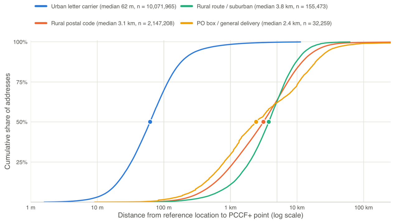
Figure 2.
Median positional error (A) and percentage of addresses with a misclassified material deprivation quintile (B), by delivery mode and rurality of the reference location. Cells marked n<100 contain fewer than 100 addresses and are not shown; cells marked none contain no addresses. LC, letter carrier.
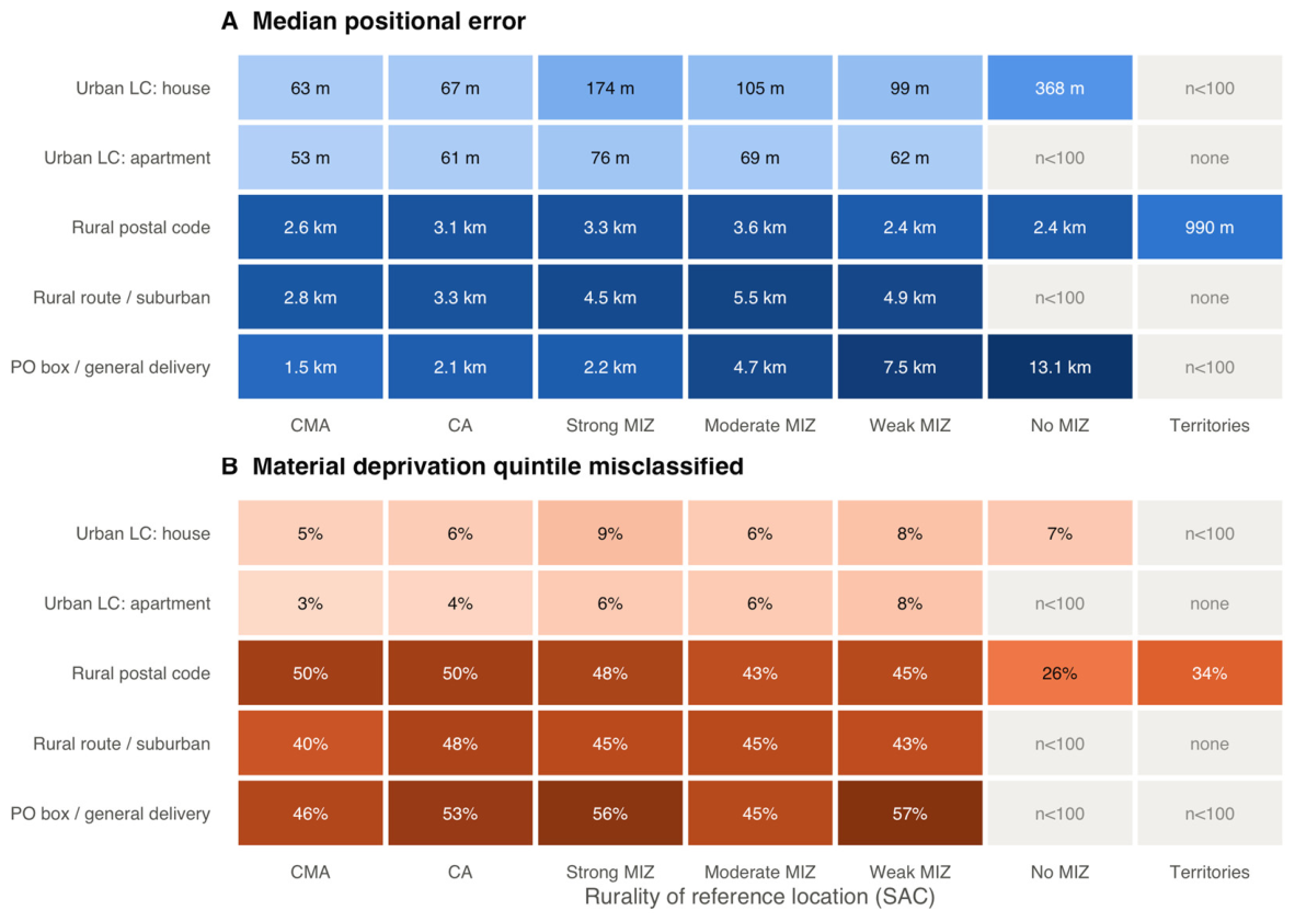
Figure 3.
Growing-season EVI (2025–2026 mean, 3 × 3 cell window) at the reference location and at the PCCF+ point for urban letter-carrier delivery and rural postal codes. The diagonal indicates agreement; horizontal bands reflect many addresses sharing one PCCF+ point.
Figure 3.
Growing-season EVI (2025–2026 mean, 3 × 3 cell window) at the reference location and at the PCCF+ point for urban letter-carrier delivery and rural postal codes. The diagonal indicates agreement; horizontal bands reflect many addresses sharing one PCCF+ point.
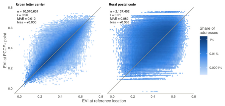
Figure 4.
Material deprivation quintile at the reference location (rows) and at the PCCF+ point (columns), as row percentages, for urban letter-carrier delivery and rural postal codes.
Figure 4.
Material deprivation quintile at the reference location (rows) and at the PCCF+ point (columns), as row percentages, for urban letter-carrier delivery and rural postal codes.
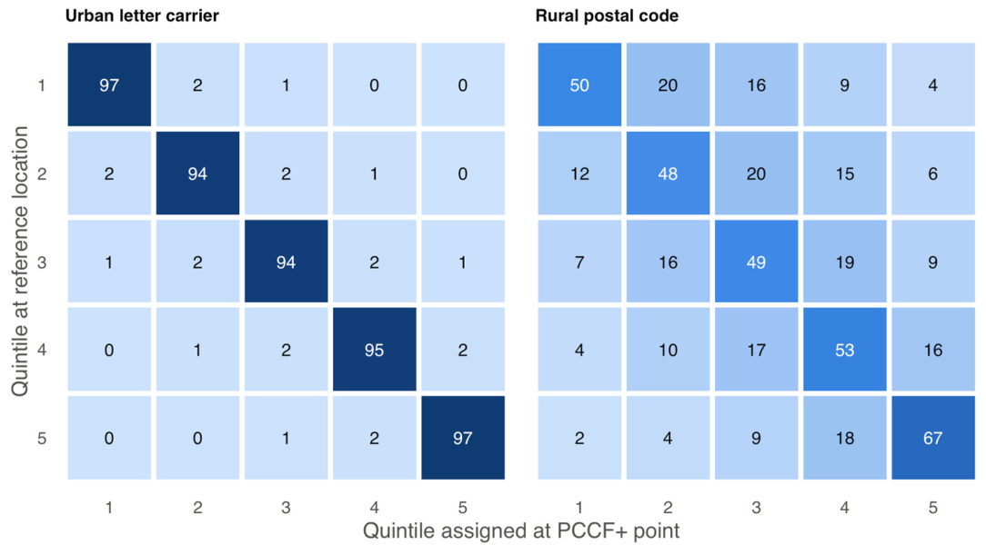
Figure 5.
Rate ratios by material deprivation quintile in a synthetic cohort of 50,000 rural Ontario addresses with a population rate ratio of 2.0 between the fifth and first quintiles (grey line), estimated naively from the assigned quintile and with the stratum and postal-code corrections. Because outcomes were simulated, the realized ratio in this cohort was 1.68, against which the estimates of 1.31 (naive), 1.33 (stratum correction by province, SAC type and delivery mode) and 1.67 (postal code) can be compared. Bars show 95% intervals: a confidence interval for the naive estimate, a simulation interval for the stratum correction and a credible interval for the postal-code correction.
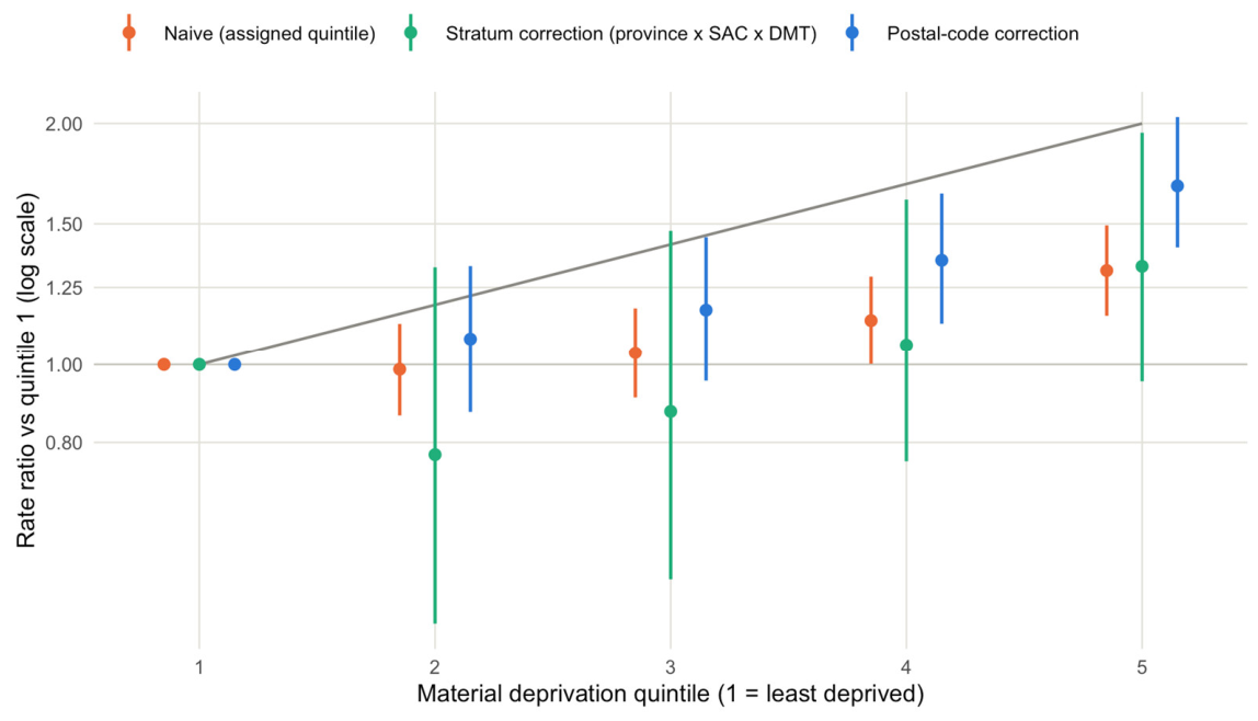

Table 1.
Characteristics of the primary residential address sample (n = 12,412,300).
| Characteristic | Addresses (n) | % |
|---|---|---|
| Reference source | ||
| NAR building point | 11,675,690 | 94.1 |
| Open Database of Addresses point | 250,084 | 2.0 |
| NAR blockface point | 486,526 | 3.9 |
| Delivery mode | ||
| Urban, house (A) | 7,989,501 | 64.4 |
| Urban, apartment (B) | 2,052,235 | 16.5 |
| Business or LVR (E, G) | 30,229 | 0.2 |
| Rural postal code (W) | 2,147,208 | 17.3 |
| Rural route or suburban (H, T) | 155,473 | 1.3 |
| PO box or GD (J, K, M, R, X) | 32,259 | 0.3 |
| Unknown or retired (Z) | 5,395 | 0.0 |
| Rurality (SAC) | ||
| CMA | 8,762,617 | 70.6 |
| CA | 1,413,385 | 11.4 |
| Strong MIZ | 739,818 | 6.0 |
| Moderate MIZ | 931,213 | 7.5 |
| Weak MIZ | 511,041 | 4.1 |
| No MIZ | 44,111 | 0.4 |
| Territories | 10,115 | 0.1 |
Percentages are calculated within each block. LVR, large volume receiver; PO, post office; GD, general delivery; SAC, Statistical Area Classification; CMA, census metropolitan area; CA, census agglomeration; MIZ, census metropolitan influenced zone. Delivery mode type codes in parentheses.
Table 2.
Positional error of PCCF+ and agreement of assigned census areas with the reference location, by delivery mode and rurality.
Table 2.
Positional error of PCCF+ and agreement of assigned census areas with the reference location, by delivery mode and rurality.
| Group | n | Median (m) | IQR (m) | P90 (m) | ≤100 m (%) | >5 km (%) | Same DA (%) | Same CSD (%) |
|---|---|---|---|---|---|---|---|---|
| All addresses | 12,412,300 | 81 | 38–240 | 3,073 | 56.8 | 7.1 | 80.6 | 96.7 |
| Delivery mode | ||||||||
| Urban, house | 7,989,501 | 65 | 33–124 | 233 | 67.3 | 0.3 | 91.8 | 99.8 |
| Urban, apartment | 2,052,235 | 53 | 30–89 | 141 | 79.8 | 0.1 | 94.7 | 99.8 |
| Business or LVR | 30,229 | 48 | 28–82 | 149 | 82.4 | 0.3 | 92.2 | 99.8 |
| Rural postal code | 2,147,208 | 3,125 | 1131–7242 | 13,625 | 0.6 | 36.3 | 29.6 | 83.6 |
| Rural route or suburban | 155,473 | 3,759 | 1922–6596 | 10,781 | 0.3 | 37.0 | 36.9 | 86.1 |
| PO box or GD | 32,259 | 2,429 | 804–10660 | 21,724 | 1.7 | 37.9 | 21.6 | 84.0 |
| Unknown or retired | 5,395 | 2,771 | 1592–7967 | 22,569 | 2.3 | 32.0 | 9.1 | 60.4 |
| Rurality (SAC) | ||||||||
| CMA | 8,762,617 | 63 | 33–120 | 256 | 68.6 | 1.6 | 89.6 | 99.3 |
| CA | 1,413,385 | 84 | 39–247 | 2,330 | 55.4 | 5.8 | 81.2 | 97.9 |
| Strong MIZ | 739,818 | 2,368 | 668–5787 | 10,388 | 7.5 | 29.4 | 39.6 | 88.0 |
| Moderate MIZ | 931,213 | 2,093 | 414–6743 | 14,387 | 12.4 | 31.7 | 46.9 | 84.2 |
| Weak MIZ | 511,041 | 1,045 | 208–4866 | 13,413 | 16.8 | 24.6 | 48.2 | 87.5 |
| No MIZ | 44,111 | 2,218 | 532–8793 | 17,542 | 2.9 | 35.1 | 54.8 | 61.6 |
| Territories | 10,115 | 1,014 | 516–2207 | 4,840 | 2.5 | 9.6 | 48.5 | 93.2 |
IQR, interquartile range; P90, 90th percentile; DA, dissemination area; CSD, census subdivision; LVR, large volume receiver; PO, post office; GD, general delivery. Delivery mode type codes are given in Table 1.
Table 3.
Agreement of greenness (EVI, 3 × 3 window, 2025–2026 mean) and deprivation quintiles (MSDI, 2021) assigned at the PCCF+ point with values at the reference location, by delivery mode.
Table 3.
Agreement of greenness (EVI, 3 × 3 window, 2025–2026 mean) and deprivation quintiles (MSDI, 2021) assigned at the PCCF+ point with values at the reference location, by delivery mode.
| Delivery mode | EVI bias | EVI MAE | EVI r | Mat. MC (%) | Soc. MC (%) | Mat. ≥2 Q (%) | κ mat. | κ soc. |
|---|---|---|---|---|---|---|---|---|
| Urban, house | 0.000 | 0.013 | 0.96 | 5.0 | 4.9 | 1.7 | 0.95 | 0.95 |
| Urban, apartment | 0.000 | 0.010 | 0.97 | 2.9 | 2.9 | 1.1 | 0.97 | 0.95 |
| Business or LVR | +0.001 | 0.009 | 0.98 | 3.1 | 2.8 | 2.0 | 0.96 | 0.95 |
| Rural postal code | +0.036 | 0.082 | 0.51 | 46.2 | 48.8 | 17.7 | 0.52 | 0.39 |
| Rural route or suburban | +0.035 | 0.082 | 0.37 | 43.6 | 40.8 | 18.7 | 0.51 | 0.47 |
| PO box or GD | +0.007 | 0.071 | 0.61 | 51.0 | 53.5 | 24.5 | 0.42 | 0.44 |
| Unknown or retired | +0.029 | 0.082 | 0.38 | 65.7 | 57.5 | 30.7 | 0.27 | 0.40 |
Bias and MAE (mean absolute difference) are PCCF+ minus reference, in EVI units; r, Pearson correlation; Mat., material; Soc., social; MC, misclassified (quintile at the PCCF+ dissemination area differs from the quintile at the reference dissemination area); ≥2 Q, misclassified by two or more quintiles; κ, linearly weighted kappa; LVR, large volume receiver; PO, post office; GD, general delivery. Delivery mode type codes are given in Table 1.
Table 4.
Percentage of residential addresses whose material deprivation quintile (MSDI 2021) assigned by PCCF+ differs from the quintile at the reference location, by province and delivery mode type (DMT) of the postal code.
Table 4.
Percentage of residential addresses whose material deprivation quintile (MSDI 2021) assigned by PCCF+ differs from the quintile at the reference location, by province and delivery mode type (DMT) of the postal code.
| Province | House (A) | Apartment (B) | Business (E, G) | Rural (W) | Rural route (H, T) | PO box, GD (J, K, M) | All |
|---|---|---|---|---|---|---|---|
| NL | 6.9 | 8.8 | 0.0† | 19.9 | 34.6 | 13.1† | 12.1 |
| PE | 2.5 | 9.9 | – | 55.2 | 68.2† | 56.8† | 32.1 |
| NS | 5.3 | 3.1 | 0.0† | 47.5 | 50.0 | 35.0† | 20.8 |
| NB | 3.3 | 4.2 | 0.0† | – | 23.1† | 20.2† | 3.4 |
| QC | 4.0 | 2.4 | 1.8 | 40.6 | 34.6 | 45.3 | 11.5 |
| ON | 5.4 | 2.8 | 3.1 | 53.4 | 46.3 | 54.5 | 13.3 |
| MB | 3.8 | 3.9 | 1.0† | 41.4 | 48.4 | 71.3 | 11.7 |
| SK | 3.2 | 3.2 | 21.0† | 48.1 | 31.7† | 39.2† | 15.9 |
| AB | 5.3 | 3.0 | 0.1 | 53.8 | 44.4 | 49.1 | 11.3 |
| BC | 6.4 | 3.1 | 4.7 | 42.1 | 47.1 | 50.4 | 10.3 |
| YT | 3.2 | 29.9† | – | 30.2 | 100.0† | – | 11.2 |
| NT | 5.0 | 0.0† | 0.0† | 36.8 | – | 100.0† | 14.6 |
| NU | – | – | – | 35.2 | – | – | 35.2 |
| Canada | 4.9 | 2.9 | 3.0 | 46.2 | 43.6 | 51.0 | 12.3 |
† Fewer than 1,000 addresses. – No addresses. GD, general delivery. Delivery mode types with retired or unknown codes (Z) are included in All. Error measures by province and delivery mode, and by province and SAC type, with weighted kappa, score error and calibration slopes, are given in Table S5.
Table 5.
Validation of the correction methods: percentage bias of the geometric mean rate ratio between the fifth and first material deprivation quintiles (true value 2.0) and coverage of its 95% interval.
Table 5.
Validation of the correction methods: percentage bias of the geometric mean rate ratio between the fifth and first material deprivation quintiles (true value 2.0) and coverage of its 95% interval.
| Scenario | Naive | Province × SAC | Province × DMT | Province × SAC × DMT | Postal code | Oracle |
|---|---|---|---|---|---|---|
| S1 National | −5.5 / 68 | −0.5 / 98 | 0.0 / 96 | −1.1 / 94 | −0.6 / 93 | −0.2 / 96 |
| S2 Rural | −21.1 / 24 | −6.3 / 95 | −8.6 / 95 | −7.7 / 93 | −1.6 / 97 | −1.9 / 98 |
| S3 Clustered | −5.0 / 92 | −1.8 / 95 | −1.6 / 96 | −3.1 / 94 | −0.2 / 95 | −0.1 / 96 |
| S4 Deprived cohort | −9.9 / 61 | −5.9 / 88 | −5.7 / 90 | −8.4 / 82 | −2.2 / 92 | −1.0 / 96 |
| S5 Rural Saskatchewan | −30.9 / 11 | −6.7 / 97 | −14.3 / 93 | −2.6 / 98 | −2.3 / 92 | −2.6 / 98 |
| Cohorts with an atypical delivery-mode mix | ||||||
| K1 Urban delivery in MIZ | −4.7 / 92 | +16.4 / 80 | +1.7 / 90 | +2.1 / 92 | −1.3 / 100 | −0.9 / 98 |
| K2 Rural delivery in CMA/CA | −23.8 / 5 | −23.1 / 22 | −0.5 / 95 | −9.8 / 88 | +1.3 / 92 | +1.6 / 92 |
Values are bias (%) / coverage (%). Naive, by assigned quintile; Province × SAC, Province × DMT and Province × SAC × DMT, stratum correction with the stated strata, DMT grouped as urban letter carrier, rural or other (postal-code split validation; 200 Monte Carlo draws; 95% simulation interval); Postal code, Gibbs data augmentation with postal-code quintile distributions (address split validation; 95% credible interval); Oracle, by true quintile. Naive and oracle intervals are 95% confidence intervals. S1–S5: 100 cohorts each; K1–K2: 40 cohorts each; the Monte Carlo standard error of coverage near 95% is about 2 points with 100 cohorts and 3.5 points with 40. Naive, postal-code and oracle results are from the same cohorts.
Disclaimer/Publisher’s Note: The statements, opinions and data contained in all publications are solely those of the individual author(s) and contributor(s) and not of MDPI and/or the editor(s). MDPI and/or the editor(s) disclaim responsibility for any injury to people or property resulting from any ideas, methods, instructions or products referred to in the content. |
© 2026 by the authors. Licensee MDPI, Basel, Switzerland. This article is an open access article distributed under the terms and conditions of the Creative Commons Attribution (CC BY) license (http://creativecommons.org/licenses/by/4.0/).
Copyright: This open access article is published under a Creative Commons CC BY 4.0 license, which permit the free download, distribution, and reuse, provided that the author and preprint are cited in any reuse.