

Submitted:
10 October 2026
Posted:
13 October 2026
You are already at the latest version
Abstract
Adaptive gradient clipping can improve training without establishing that its feedback signals are useful. We examine Dynamics-Aware Gradient Clipping (DAGC), a bounded threshold controller driven by clipping exposure and consecutive-gradient alignment. Its exposure term tightens clipping when clipping is already frequent. We show that an interior target-exposure equilibrium is unstable in a stationary mean-field model, even with exponential smoothing. We then compare the frozen controller with tuned clipping rules, an alignment ablation, and a predetermined threshold schedule on FashionMNIST and CIFAR-10, using validation-only calibration and twelve paired confirmation seeds in each of three conditions.These controls separate threshold scheduling from evidence for an online feedback mechanism; the analysis does not claim convergence of the coupled training dynamics.
Keywords:
gradient clipping
; adaptive optimization
; feedback control
; threshold scheduling
; gradient alignment
; training stability
1. Introduction
Gradient clipping limits the contribution of a large gradient to an optimizer update [1]. A fixed threshold is simple but introduces a scale-sensitive hyperparameter. Adaptive rules can instead derive a threshold from gradient history or parameter magnitude [2,3]. When an adaptive method succeeds, however, its accuracy alone does not establish why: a useful threshold profile, a smaller effective step size, and informative feedback can produce similar outcomes.
We examine that ambiguity in Dynamics-Aware Gradient Clipping (DAGC). The controller uses the recent frequency of clipping and the alignment of consecutive raw gradients. Its first version, V1, allowed exposure alone to increase the threshold but not decrease it. V2 replaces that one-sided term with a term that becomes negative above a reference exposure. This makes sustained clipping more restrictive. It also gives the feedback the opposite sign to a clipping-rate tracker: lowering a threshold makes further clipping more likely.
This distinction changes both the interpretation and the experiment needed to support the method. A comparison with an arbitrary fixed threshold cannot establish that exposure or alignment provides useful information beyond the gradient scale. Removing the alignment term tests its necessity. A lagged median rule tests whether magnitude information is sufficient. Replaying a threshold trace constructed on separate calibration runs tests the incremental value of adapting that threshold to the new training trajectory. Replay still uses the current norm to apply clipping; only its threshold is predetermined.
Our contribution is an analysis and controlled evaluation of this concrete controller. First, we derive its local positive-feedback behavior with the exposure EMA included. Second, we define a reproducible comparison with validation-only parameter selection, identical paired training streams, and explicit failure accounting. Third, we preserve the earlier negative mechanism controls and evaluate transfer to longer training and a residual network on RGB images. The scope is small image classifiers trained with momentum SGD; there is no claim of broad optimizer, architecture, or language-model transfer.
2. Related Work
Adaptive gradient and update clipping.
Fixed norm clipping was popularized for recurrent-network optimization [1]. AutoClip derives a global threshold from historical norm percentiles [2]; AGC instead uses unit-wise parameter magnitude [3]. ACClip uses coordinate-wise adaptation in attention models [4]. ZClip detects norm spikes through running statistics [5], whereas the revised AdaGC bounds tensor gradients relative to historical clipped-norm estimates [6]. Group-level historical control also appears in AGGC [7]. These rules differ in granularity, reference scale, and treatment of anomalous gradients. DAGC uses one global threshold with exposure and consecutive-gradient alignment; its distinction must be tested against these simpler information sources, not inferred from the general novelty of an adaptive threshold.
Clippy constrains optimizer updates in multitask ranking [8]. This distinction matters because raw-gradient clipping does not directly bound the parameter step after momentum or preconditioning. StableAdamW addresses underestimated second-moment states in vision-language training [9]. Such optimizer-specific protections motivate our explicit clipping order, but their large-scale results are not experimental evidence for DAGC.
Rate feedback, quantiles, and robust estimation.
Adaptive private federated clipping estimates a desired norm quantile online [10]. Quantile clipping has also been studied through robust stochastic optimization [11] and adaptive DP-SGD convergence analysis [12]. These analyses highlight clipping bias and the joint role of threshold and stepsize schedules. The geometric treatment of private SGD likewise shows that clipping can bias an update [13]. DAGC is neither a privacy mechanism nor a quantile estimator: its excess-exposure response has the opposite sign to rate tracking. Median-gradient estimators connect some clipping methods to robust location estimation [14], but estimating a median gradient vector is distinct from our scalar rolling-median norm control.
Optimization theory and heavy-tailed noise.
Relaxed-smoothness analyses explain why clipping can accelerate optimization [15,16]. Stability and convergence results also cover rapidly growing subgradients and clipped momentum [17]. Stochastic bias can limit convergence even when clipping prevents large updates [18]. Empirical tail-index studies [19] and attention-model analysis [4] motivate considering non-Gaussian gradient noise. Accelerated clipping and normalized clipped momentum provide heavy-tail guarantees under stated assumptions [20,21]; newer work separates the roles of normalization and clipping [22]. We neither estimate a tail index nor verify these assumptions for our networks. These results supply context, not a convergence theorem for the DAGC controller coupled to neural-network training.
Adaptation, architecture, and training scale.
AdaGrad [23] and AdaGrad-Norm [24] adapt step scales using past gradients; Adam [25] adds coordinate-wise moment estimates. AdamW separates weight decay from its adaptive update [26], while LAMB uses layer-wise update scaling [27]. These are alternative ways to change update magnitude rather than evidence that a specific clipping feedback signal is informative. Initialization and momentum also materially affect optimization [28,29]. Batch normalization [30,31] and residual connections [32] change the training setting, so gains on a small CNN cannot automatically transfer to a residual model. Small-scale Transformer proxies reproduce selected instabilities under explicit conditions [33]; our image experiments do not establish a corresponding language-model transfer claim.
Evidence for a mechanism.
Benchmark variance [34], selection bias [35], and finite hyperparameter-search budgets [36] motivate paired seeds and validation-only selection. Freshly collected benchmark tests can change absolute scores [37]; withholding a test set during the new campaign does not erase earlier exposure to it. Statistical comparisons must respect the replication unit and test assumptions [38]. We distinguish descriptive legacy evidence, multiplicity-corrected confirmation [39], and equivalence within a stated practical margin [40]. This prevents a null replay comparison from being presented either as proof of superiority or as proof of equivalence.
3. Controller and Competing Explanations
Let be the raw minibatch gradient, and let . A positive threshold gives
We log exposure , intensity , and alignment . The first alignment is one. The exposure and alignment states are
initialized at and . DAGC-V2 updates
Here and , where is the lower median of the last 200 raw gradient norms, including . Thus these bounds affect the next step. The frozen settings are . V1 replaces with ; since , its exposure term cannot itself tighten clipping. V2 can tighten, but this change alone does not imply useful regulation.
| Algorithm 1 One DAGC-V2 training step |
The ordering prevents the current norm from selecting its own DAGC threshold. Clipping precedes SGD’s coupled weight decay and momentum accumulation. Hence bounds the clipped data gradient, not the final parameter displacement. The method stores a previous full gradient, requiring additional memory, and a 200-element norm window. Its diagnostic alignment requires an dot product. We do not describe it as constant-memory control.
3.1. The Reference Exposure Is Not a Stable Target
For a stationary, exogenous gradient-norm distribution, with alignment disabled and inactive bounds, the exposure-EMA mean-field system has a linearly unstable interior reference-exposure fixed point whenever the density at that threshold is positive. Appendix F gives the assumptions, Jacobian and complete proof, together with conditional results on alignment masking and replay.
The result includes exposure smoothing; an EMA does not reverse the feedback sign. It does not prove instability of neural-network training: the gradient norm distribution changes with the parameters, the bounds move, and the alignment signal can activate. It does explain why the reference should not be interpreted as a regulated clipping frequency. Persistent clipping can instead drive the threshold to its lower bound, where historical norm scale may dominate the resulting behavior.
3.2. What Clipping Can Protect
For momentum SGD without weight decay, . If over k updates and , then
A smaller sustained threshold bounds new momentum contributions but does not remove an existing buffer. Coupled weight decay adds parameter-dependent terms. This elementary bound motivates a protection hypothesis without establishing convergence, explaining a test-accuracy improvement, or requiring exposure and alignment to be the best threshold signals.
4. Experimental Design
4.1. Questions, Conditions, and Data Separation
The new study asks whether the frozen controller outperforms tuned fixed clipping, a tuned median-scale rule, and calibration-trace replay. Its secondary question is whether removing alignment changes the outcome. The three conditions are FashionMNIST with the existing small CNN at initial learning rate , and CIFAR-10 with ResNet-20 at or . The latter two are designated lower and higher learning rates; we do not assume either one diverges without clipping.
FashionMNIST [41] uses 55,000 training images and a fixed 5,000-image validation split. CIFAR-10 [42] uses 45,000 training and 5,000 validation images. Both splits hold out 500 images per class using seed 1729. All methods train on the same remaining examples; validation images never enter training. Only calibration runs evaluate the validation set. Confirmation runs evaluate the complete official 10,000-image test set once, after the last training epoch. They retain the same training partition, preserving the number of steps used to construct replay schedules. No test score is used to choose a new-campaign hyperparameter or checkpoint.
FashionMNIST uses two convolutional layers (32 and 64 channels), max pooling, and a 128-unit hidden classifier, with 421,642 parameters. CIFAR-10 uses the 6n+2 residual architecture of He et al. [32], , widths 16/32/64, option-A shortcuts, and batch normalization, with 269,722 parameters. The RGB model is deeper, not larger in parameter count. This is an architectural transfer test, not a reproduction of the original ResNet training recipe.
4.2. Training and Calibration Budget
Training uses FP32 SGD with momentum , batch size 256, and no dropped last batch. FashionMNIST runs for 30 epochs with weight decay ; CIFAR-10 runs for 60 epochs with weight decay . A cosine schedule decreases the learning rate to 1% of its initial value. CIFAR-10 uses random padded crops and horizontal flips; FashionMNIST uses normalization only. All settings are fixed across clipping policies within a condition.
Fixed clipping, AGC, AutoClip, and the median rule each receive three candidates and three calibration seeds (2100–2102): nine runs per policy per condition. Their grids are, respectively, , , percentiles , and . The winner maximizes mean final validation accuracy, with grid order breaking exact ties. These equal finite budgets do not constitute exhaustive tuning. DAGC retains the setting selected during earlier development, so its total historical tuning budget is not matched to the new baselines.
AGC clips every parameter, grouping matrix and convolution weights by output unit and treating vectors as a single unit, with parameter-norm floor . AutoClip takes the stated percentile of all raw norms through the current step, following its authors’ convention. The median rule clips at , using available history and initial threshold 0.5. It is causal and uses the same lower-median convention as DAGC. The no-alignment variant sets without retuning. Replay averages the thresholds actually applied in three full DAGC calibration runs and applies this fixed, step-indexed schedule in confirmation. All eight policies, including no clipping, share a complete training budget.
4.3. Pairing, Failures, and Inference
Confirmation uses twelve seeds, 3100–3111. Within a seed, initial weights, minibatch order, and augmentations are identical across policies. Private random generators isolate the input stream from diagnostics and controller state. Deterministic CUDA operations are enabled and TF32 is disabled. Epoch checkpoints include model, optimizer, controller, previous raw gradient, and logs; a test verifies that resumed and uninterrupted runs agree exactly. Configuration and source checksums reject stale results.
A run stops on nonfinite loss or gradient norm, or loss above . A nonfinite final evaluation also fails. Failed runs receive accuracy zero and remain in all aggregates; finite chance-level runs retain their observed score. We do not choose the best epoch, discard failures, or rerun unfavorable seeds. The final audit checks all 117 calibration and 288 confirmation outcomes.
We report Student-t 95% intervals over seeds, including paired intervals for accuracy differences. The primary family comprises DAGC versus fixed, median, and replay in all three conditions: nine two-sided exact sign-flip tests with Holm correction. Sign flipping assumes exchangeability under the null; the t intervals assume the seed-level mean is adequately approximated by that model. Neither addresses uncertainty from sampling a new dataset. A broad superiority claim requires a positive effect and corrected significance in all nine comparisons. Secondary comparisons are descriptive.
A prespecified percentage-point margin supplies an additional within-comparison equivalence check: the paired 90% interval must lie entirely inside that range. This is not a familywise equivalence claim. Nonsignificance alone is not evidence of equivalence. The original eight-seed plan was amended to twelve during calibration, before any confirmation runs: with eight seeds, the minimum two-sided sign-flip cannot pass the first nine-test Holm threshold . The audit preserves this amendment and all identical calibration results carried forward from the first execution.
5. Results
5.1. Completeness, Failures, and Accuracy
All 405 planned outcomes pass the source/configuration, split, seed-coverage, epoch-continuity, calibration-selection, and replay-construction audits. There are 397 full-budget completions and eight predefined scientific failures, with no process errors. All eight failures occur without clipping on FashionMNIST. Its four remaining unclipped runs finish at 10% accuracy; retaining failures at zero gives a mean of 3.33%. Every clipped confirmation run and every CIFAR-10 run completes its budget.
Table 1 reports the full comparison. On FashionMNIST, DAGC reaches 92.41%, versus 92.60% for tuned fixed clipping and 92.56% for the tuned median rule. On CIFAR-10 at LR 0.1, DAGC reaches 89.50%, versus 90.67% for fixed clipping. At LR 0.4, the corresponding scores are 90.87% and 91.16%. AGC attains the highest observed mean at the higher CIFAR rate, 91.20%; differences among non-DAGC baselines are not a prespecified hypothesis family.
The paired DAGC-minus-fixed effects are , , and points, with Holm-adjusted p-values 0.0176, 0.0044, and 0.0103, respectively (Table 2). Thus the new study reverses the earlier exploratory fixed-baseline advantage. These are different data sizes, schedules, and calibration budgets, so this is a failure of transfer under the new protocol, not a claim that the earlier measurements were numerically false. The prespecified broad-superiority criterion is not met.
At CIFAR-10 LR 0.1, calibration selects fixed threshold 5.0, and this threshold never binds in confirmation. Its norm traces and coefficients exactly match no clipping. Accordingly, the 1.17-point deficit is also a deficit to the unmodified optimizer. At LR 0.4, DAGC exceeds no clipping by 0.52 points [0.25, 0.79], but stronger performance is achieved by the tuned fixed rule. Avoiding divergence or improving on no clipping is therefore insufficient evidence for the particular DAGC controller.
5.2. Replay and Alignment Controls
DAGC-minus-replay differences are , , and points. Their paired 90% intervals are [, 0.11], [, 0.25], and [, 0.04]. Each lies inside the prespecified point margin. This supports equivalence within each tested condition at that tolerance; it is not a multiplicity-adjusted familywise equivalence result, nor a claim that the methods coincide outside these settings. The corresponding 95% intervals appear in Table 2 and Figure 1.
Removing alignment changes FashionMNIST accuracy by points in DAGC’s favor, with a paired 95% interval [, 0.33]. On both CIFAR-10 conditions, all twelve paired raw-gradient norms, applied thresholds, coefficients, alignment traces, and lower-bound indicators are exactly equal between DAGC and the no-alignment variant. The complete-trace audit shows that negative smoothed alignments do occur; the direction term is therefore not intrinsically inactive. All 3,860 negative-alignment-EMA updates across the two CIFAR conditions are projected to the lower bound. Its effect on the applied threshold is masked by lower-bound projection in these runs. This identifies a limit of the implemented controller, rather than demonstrating that gradient direction never matters.
5.3. The Lower Bound Dominates the Controller
DAGC’s next-step threshold equals its moving lower bound on 97.18%, 99.07%, and 99.00% of updates, respectively. Its mean clipping intensities are 0.893, 0.900, and 0.899. Figure 2 shows the resulting profiles. These measurements are consistent with the positive-feedback calculation: clipping stays active and the projection frequently determines the threshold.
The validation-selected median coefficient is 0.1 on FashionMNIST, matching DAGC’s lower-bound scale, and 0.4 on both CIFAR conditions. The CIFAR median rule therefore retains larger gradients, with intensities near 0.60. DAGC falls below it by 1.08 points at LR 0.1 (Holm ) and 0.21 points at LR 0.4 (Holm ). The latter comparison does not pass the primary multiplicity criterion. Bound occupancy describes which part of the rule is active; by itself it does not prove that changing only the bound would produce a particular accuracy gain.
5.4. Earlier Exploratory Evidence and Corrected Interpretation
The corresponding audited historical plots are retained in Appendix C.1; they are distinct from the confirmation evidence in Figure 1 and Figure 2.
The earlier 15-epoch, 5,000-training/2,000-test experiments used different training seeds for development and evaluation, but sampled from the same official test set for both stages. We therefore classify them as exploratory, not independent data-held-out confirmation. Their positive comparisons to fixed clipping motivated the present study; they cannot substitute for it.
The most discriminating legacy experiment already limited the mechanism claim. Over eight paired seeds, DAGC exceeded an intensity-matched fixed rule by 1.18 points (recomputed 95% paired interval [0.62, 1.74]), but its advantage over replay was 0.21 points [, 0.86]. Removing alignment changed accuracy by 0.16 points [, 0.66], whereas removing exposure cost 5.47 points [4.04, 6.90]. These results identify the effect of specified ablations on the whole training trajectory. They do not show that reversal predicts future loss deterioration or that online feedback adds value beyond replay.
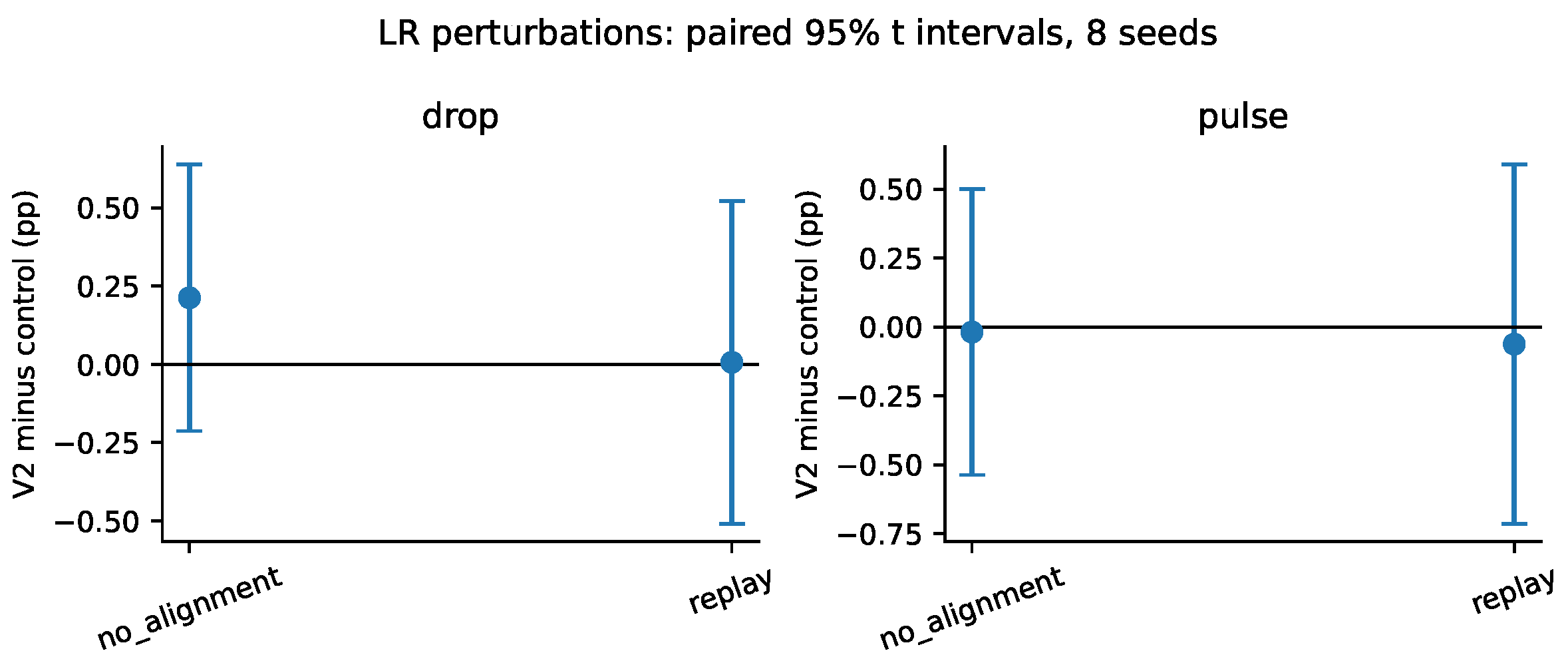
Independent-seed learning-rate perturbations did not resolve the ambiguity: the DAGC-minus-replay difference was [, 0.59] for a temporary learning-rate doubling and [, 0.52] for a sustained decrease. The uncertainty spans effects beyond the new equivalence margin, so these legacy null results are not equivalence claims. Appendix C reports all controls and corrected intervals.
A development sweep over the reference exposure had previously pooled two gains and three seeds into six apparent replicates. We instead report each gain separately with three seeds. Realized exposure remains at least 0.999 across the grid, while intensity changes. The sweep is consistent with the positive-feedback interpretation, but its small sample and development role preclude precise claims of performance insensitivity.
6. Discussion and Limitations
A controller can influence an optimization trajectory without the proposed feedback signal being necessary for its gains. The replay comparison removes threshold adaptation to the confirmation trajectory; the median comparison retains online magnitude information but removes exposure and alignment; and the no-alignment comparison removes only direction. Their scopes differ, so no single one is a complete mechanistic explanation.
The evidence supports a narrow negative conclusion about the frozen V2 rule: it does not outperform a validation-tuned fixed threshold in any of the three conditions, and its threshold adaptation adds no practically resolved advantage over calibration replay under the stated margin. The lower bound accounts for nearly all threshold updates, while its directional adjustments are masked by projection on CIFAR-10. Calling these runs successful target tracking or evidence that online directional feedback is necessary would contradict the controls. They instead show how an apparently dynamic controller can behave mostly as a historical-scale clipping rule.
The FashionMNIST and higher-rate CIFAR fixed-baseline gaps are statistically resolved but smaller than 0.5 points. Statistical inferiority can coexist with practical equivalence at a specified tolerance; the larger low-rate CIFAR gap falls outside that tolerance. The finding should guide subsequent research toward identifying conditions where feedback is informative, rather than retuning the present confirmation runs after observing their test scores.
The study remains limited to two image datasets, two small architectures, one optimizer, and fixed learning-rate schedules. Sixty CIFAR epochs are longer than the legacy diagnostics but do not establish asymptotic performance or large-scale training stability. Fixed grids can miss better baseline settings. Historical FashionMNIST test exposure and unequal earlier method development remain limitations despite validation-only selection in the new campaign. Seed intervals are conditional on a fixed data split. Our analytic model freezes the norm distribution; its unstable controller equilibrium is not a theorem about the nonlinear coupled training system. Likewise, lower-bound occupancy and accuracy correlation cannot identify a causal mechanism alone.
Appendix F proves conditional results on projection masking, exact same-run replay, and the value of causal information. These results do not establish that DAGC realizes an optimal feedback policy or outperforms independent-calibration replay; the confirmation results do not support either claim.
7. Conclusion
DAGC-V2 implements positive exposure feedback, not stable target-rate tracking in the stationary mean-field model. A useful empirical claim must therefore survive comparisons with magnitude-only adaptation and a predetermined threshold schedule, in addition to tuned fixed clipping. Our protocol makes those comparisons explicit, preserves failure outcomes, and separates legacy exploration from current validation-only selection.
Across all 405 audited runs, the frozen controller fails the broad-superiority criterion and loses to tuned fixed clipping in each confirmation condition. Replay meets the prespecified per-condition equivalence criterion, while the complete CIFAR traces show that lower-bound projection masks the alignment term. Together, these controls limit the evidence for the proposed feedback signals in these tests. These results delimit the method’s empirical claim and provide a reproducible example of separating threshold scheduling from evidence for an online feedback mechanism.
Impact Statement
This work examines optimization behavior in small image classifiers. It does not deploy a model or introduce a new dataset. Better-controlled evaluation can reduce wasted experiments and unsupported claims about training stability. A clipping rule is not a guarantee of reliable or safe behavior in downstream applications; broader deployment consequences depend on the model and use.
Appendix A. Reproducibility and Complete Calibration
The complete code, compact evidence, and manuscript are available at https://github.com/alexsongyzs-dotcom/Dynamics_Aware_Gradient_Clipping/tree/develop/yzs. The completed confirmation protocol is in docs/lyx1_protocol.md; seed-level records and audit hashes are in results/lyx1/evidence/. The original full-resolution server archive is required to rerun exact trace equality checks; binned exports alone cannot establish those equalities.
The machine-readable protocol fixes conditions, hyperparameter grids, calibration and confirmation seeds, and comparison families before confirmation. The source/configuration digest is checked when a run is resumed or reused. The evidence export verifies every run identity, exact confirmation seed sets, completed epoch continuity, and failure accounting. It retains per-epoch training metrics, final evaluation scores, 100-bin diagnostic traces, full replay schedules, and checksums for the full-resolution traces archived with the raw experiment. Tables and figures are generated from the exported seed-level records; summary values are not entered by hand.
Training inputs are cached on the GPU. CIFAR crop offsets and flips use a private generator keyed by training seed and epoch; a separate generator controls the permutation of training examples. No dropout or other random model operation is used. Model initialization uses the training seed. Exact resume tests cover optimizer state, controller state, prior gradient, metrics, and diagnostic traces. The numerical epsilon in scalar clipping is ; AGC’s parameter floor is . CUDA determinism is requested explicitly.

Table A1.
Shared implementation details.
| Item | FashionMNIST | CIFAR-10 |
|---|---|---|
| Training / validation / test | 55,000 / 5,000 / 10,000 | 45,000 / 5,000 / 10,000 |
| Epochs / updates | 30 / 6,450 | 60 / 10,560 |
| Model / parameters | SmallCNN / 421,642 | ResNet-20 / 269,722 |
| Batch / SGD momentum | 256 / 0.9 | 256 / 0.9 |
| Weight decay | ||
| Mean | 0.286 | (0.4914, 0.4822, 0.4465) |
| Standard deviation | 0.353 | (0.2470, 0.2435, 0.2616) |
| Augmentation | None | Padded crop and horizontal flip |
| Evaluation frequency | Final epoch only | Final epoch only |
Table A2.
Complete calibration grid. Each candidate uses the same three seeds. Entries list candidate: mean validation accuracy (percent). The final column is selected before confirmation.
Table A2.
Complete calibration grid. Each candidate uses the same three seeds. Entries list candidate: mean validation accuracy (percent). The final column is selected before confirmation.
| Condition / initial LR | Policy | Candidate scores | Selected |
|---|---|---|---|
| FashionMNIST / 0.8 | Tuned fixed | 0.05: 93.04, 0.5: 90.32, 5: 10.00 | 0.05 |
| FashionMNIST / 0.8 | Tuned AGC | 0.005: 93.10, 0.03: 63.57, 0.18: 10.00 | 0.005 |
| FashionMNIST / 0.8 | Tuned AutoClip | 1: 90.89, 10: 90.33, 50: 36.63 | 1 |
| FashionMNIST / 0.8 | Tuned median scale | 0.025: 91.94, 0.1: 93.06, 0.4: 91.17 | 0.1 |
| CIFAR-10 / 0.1 | Tuned fixed | 0.05: 77.25, 0.5: 91.16, 5: 91.64 | 5 |
| CIFAR-10 / 0.1 | Tuned AGC | 0.005: 84.25, 0.03: 90.31, 0.18: 91.51 | 0.18 |
| CIFAR-10 / 0.1 | Tuned AutoClip | 1: 91.34, 10: 91.51, 50: 91.48 | 10 |
| CIFAR-10 / 0.1 | Tuned median scale | 0.025: 87.73, 0.1: 90.61, 0.4: 91.17 | 0.4 |
| CIFAR-10 / 0.4 | Tuned fixed | 0.05: 88.76, 0.5: 92.01, 5: 91.26 | 0.5 |
| CIFAR-10 / 0.4 | Tuned AGC | 0.005: 83.66, 0.03: 91.57, 0.18: 91.45 | 0.03 |
| CIFAR-10 / 0.4 | Tuned AutoClip | 1: 91.44, 10: 91.63, 50: 91.44 | 10 |
| CIFAR-10 / 0.4 | Tuned median scale | 0.025: 89.85, 0.1: 91.91, 0.4: 92.03 | 0.4 |
Appendix B. Failures and Clipping Diagnostics
For global clipping, the logged coefficient is the scalar multiplier. AGC instead logs the ratio of the whole clipped-gradient norm to the raw norm; its value does not imply a global scalar intervention, since individual units receive different multipliers. Frequency counts ratios below . Intensity is one minus that ratio. Bound occupancy counts whether the newly computed DAGC threshold equals its lower bound to relative tolerance . For other policies this diagnostic is zero by construction and does not imply that their thresholds are unconstrained.
Table A3.
Failures and mean diagnostics across twelve seeds. f is clipping frequency, I is intensity, and b is lower-bound occupancy.
Table A3.
Failures and mean diagnostics across twelve seeds. f is clipping frequency, I is intensity, and b is lower-bound occupancy.
| Condition / initial LR | Policy | Failed | f | I | b |
|---|---|---|---|---|---|
| FashionMNIST / 0.8 | No clipping | 8/12 | 0.000 | 0.000 | 0.000 |
| FashionMNIST / 0.8 | Tuned fixed | 0/12 | 1.000 | 0.947 | 0.000 |
| FashionMNIST / 0.8 | Tuned AGC | 0/12 | 1.000 | 0.941 | 0.000 |
| FashionMNIST / 0.8 | Tuned AutoClip | 0/12 | 0.954 | 0.297 | 0.000 |
| FashionMNIST / 0.8 | Tuned median scale | 0/12 | 1.000 | 0.896 | 0.000 |
| FashionMNIST / 0.8 | DAGC-V2 | 0/12 | 1.000 | 0.893 | 0.972 |
| FashionMNIST / 0.8 | No alignment | 0/12 | 1.000 | 0.893 | 0.970 |
| FashionMNIST / 0.8 | Trace replay | 0/12 | 1.000 | 0.894 | 0.000 |
| CIFAR-10 / 0.1 | No clipping | 0/12 | 0.000 | 0.000 | 0.000 |
| CIFAR-10 / 0.1 | Tuned fixed | 0/12 | 0.000 | 0.000 | 0.000 |
| CIFAR-10 / 0.1 | Tuned AGC | 0/12 | 0.763 | 0.008 | 0.000 |
| CIFAR-10 / 0.1 | Tuned AutoClip | 0/12 | 0.960 | 0.262 | 0.000 |
| CIFAR-10 / 0.1 | Tuned median scale | 0/12 | 1.000 | 0.598 | 0.000 |
| CIFAR-10 / 0.1 | DAGC-V2 | 0/12 | 1.000 | 0.900 | 0.991 |
| CIFAR-10 / 0.1 | No alignment | 0/12 | 1.000 | 0.900 | 0.991 |
| CIFAR-10 / 0.1 | Trace replay | 0/12 | 1.000 | 0.900 | 0.000 |
| CIFAR-10 / 0.4 | No clipping | 0/12 | 0.000 | 0.000 | 0.000 |
| CIFAR-10 / 0.4 | Tuned fixed | 0/12 | 1.000 | 0.585 | 0.000 |
| CIFAR-10 / 0.4 | Tuned AGC | 0/12 | 1.000 | 0.232 | 0.000 |
| CIFAR-10 / 0.4 | Tuned AutoClip | 0/12 | 0.987 | 0.355 | 0.000 |
| CIFAR-10 / 0.4 | Tuned median scale | 0/12 | 0.999 | 0.599 | 0.000 |
| CIFAR-10 / 0.4 | DAGC-V2 | 0/12 | 1.000 | 0.899 | 0.990 |
| CIFAR-10 / 0.4 | No alignment | 0/12 | 1.000 | 0.899 | 0.990 |
| CIFAR-10 / 0.4 | Trace replay | 0/12 | 1.000 | 0.900 | 0.000 |
Appendix C. Legacy Exploratory Experiments
These experiments precede the new validation-isolated protocol. Each training seed selects 5,000 official training images and 2,000 official test images; test scores were available during earlier method selection. The CNN is the same SmallCNN. Training uses 15 epochs, 300 updates, constant LR 0.8, batch 256, SGD momentum 0.9, and weight decay . Calibration seeds 800–802 construct the mean replay trace and select a fixed threshold from by matching mean clipping intensity, not accuracy. That criterion chooses 0.2. Evaluation seeds are 900–907. The new campaign instead tunes fixed clipping for validation accuracy.
Table A4.
Legacy mechanism controls, eight paired seeds. All intervals are recomputed Student-t 95% intervals, replacing the original normal approximation. is DAGC minus the listed control, in percentage points.
Table A4.
Legacy mechanism controls, eight paired seeds. All intervals are recomputed Student-t 95% intervals, replacing the original normal approximation. is DAGC minus the listed control, in percentage points.
| Policy | Accuracy (%) | Paired 95% interval | |
|---|---|---|---|
| DAGC-V2 | +0.00 | [+0.00, +0.00] | |
| No alignment | +0.16 | [-0.33, +0.66] | |
| No exposure | +5.47 | [+4.04, +6.90] | |
| Zero controller gain | +6.05 | [+4.92, +7.18] | |
| Intensity-matched fixed | +1.18 | [+0.62, +1.74] | |
| Trace replay | +0.21 | [-0.43, +0.86] | |
| AutoClip (10th percentile) | +6.92 | [+5.39, +8.45] | |
| Rate tracking | +11.59 | [+9.62, +13.56] |
“Zero controller gain” sets but retains projection onto moving norm-dependent bounds. It therefore does not implement a truly fixed threshold. The older label “frozen threshold” obscured that distinction. “No exposure” sets ; no alignment sets . AutoClip uses its tenth percentile, without a tuning search. The rate-tracking control reverses the exposure sign and removes the direction term, giving without rolling-median bounds and with the same initial threshold. It is an isolated sign-control experiment, not a replication of a private federated algorithm. These untuned configurations do not establish method-wide superiority over those algorithm families.
Table A5.
Legacy learning-rate perturbations, eight paired seeds 1000–1007. DAGC-minus-control accuracy differences in percentage points.
Table A5.
Legacy learning-rate perturbations, eight paired seeds 1000–1007. DAGC-minus-control accuracy differences in percentage points.
| Perturbation | Comparator | Difference | Paired 95% interval |
|---|---|---|---|
| Drop | No alignment | +0.21 | [-0.21, +0.64] |
| Drop | Trace replay | +0.01 | [-0.51, +0.52] |
| Pulse | No alignment | -0.02 | [-0.54, +0.50] |
| Pulse | Trace replay | -0.06 | [-0.71, +0.59] |
The pulse changes LR from 0.8 to 1.6 at zero-based step 100 and back to 0.8 at step 160. The drop changes LR from 0.8 to 0.2 at step 100 and keeps it there. The replay remains the unperturbed calibration trace. Neither condition recalibrates or resets the optimizer.
Legacy comparisons labeled ZClip or AdaGC are not used as evidence here: the correspondence of their local implementations and modified warmup to the authors’ algorithms has not been established. Their raw artifacts remain in the project history, but calling those settings “published defaults” would not be justified. The present baseline claims are limited to the explicitly defined, calibrated clipping rules in the new protocol.
Table A6.
Legacy development sweep, three seeds (200–202) per gain/reference combination. Gains are not pooled as independent replicates. Intervals reflect only within-setting seed variation and are descriptive, not selection-adjusted.
Table A6.
Legacy development sweep, three seeds (200–202) per gain/reference combination. Gains are not pooled as independent replicates. Intervals reflect only within-setting seed variation and are descriptive, not selection-adjusted.
| Gain | Reference | Accuracy (%), 95% interval | Exposure | Intensity |
|---|---|---|---|---|
| 0.05 | 0.10 | 86.83 ± 3.50 | 1.000 | 0.799 |
| 0.05 | 0.20 | 86.20 ± 2.69 | 1.000 | 0.779 |
| 0.05 | 0.35 | 86.08 ± 2.59 | 1.000 | 0.749 |
| 0.05 | 0.50 | 85.87 ± 3.39 | 1.000 | 0.716 |
| 0.05 | 0.70 | 85.85 ± 4.00 | 0.999 | 0.633 |
| 0.10 | 0.10 | 86.52 ± 3.73 | 1.000 | 0.850 |
| 0.10 | 0.20 | 86.47 ± 5.54 | 1.000 | 0.840 |
| 0.10 | 0.35 | 86.53 ± 2.76 | 1.000 | 0.827 |
| 0.10 | 0.50 | 86.12 ± 2.87 | 1.000 | 0.801 |
| 0.10 | 0.70 | 86.62 ± 2.08 | 1.000 | 0.762 |
Appendix C.1. Audited Plots of the Earlier V2 Experiments
The following plots preserve the earlier evidence without mixing it with the completed confirmation study. The benchmark campaigns used 5,000 training and 2,000 test images, 15 epochs, and eight evaluation seeds per condition. Method development had already consulted the official test distribution; fresh seeds do not remove that historical selection limitation. Figures below use audited records and seed-level Student-t intervals. Their values must not be pooled with the full-data, validation-calibrated confirmation outcomes.
Figure A1.
Earlier exploratory V2 benchmarks on four dataset/model/LR conditions. The panels preserve recorded local gains and no-clipping failures; they are not independent confirmation of an advantage over tuned baselines. The new study uses different data sizes, schedules and calibration budgets and finds DAGC inferior to tuned fixed clipping in all three conditions.
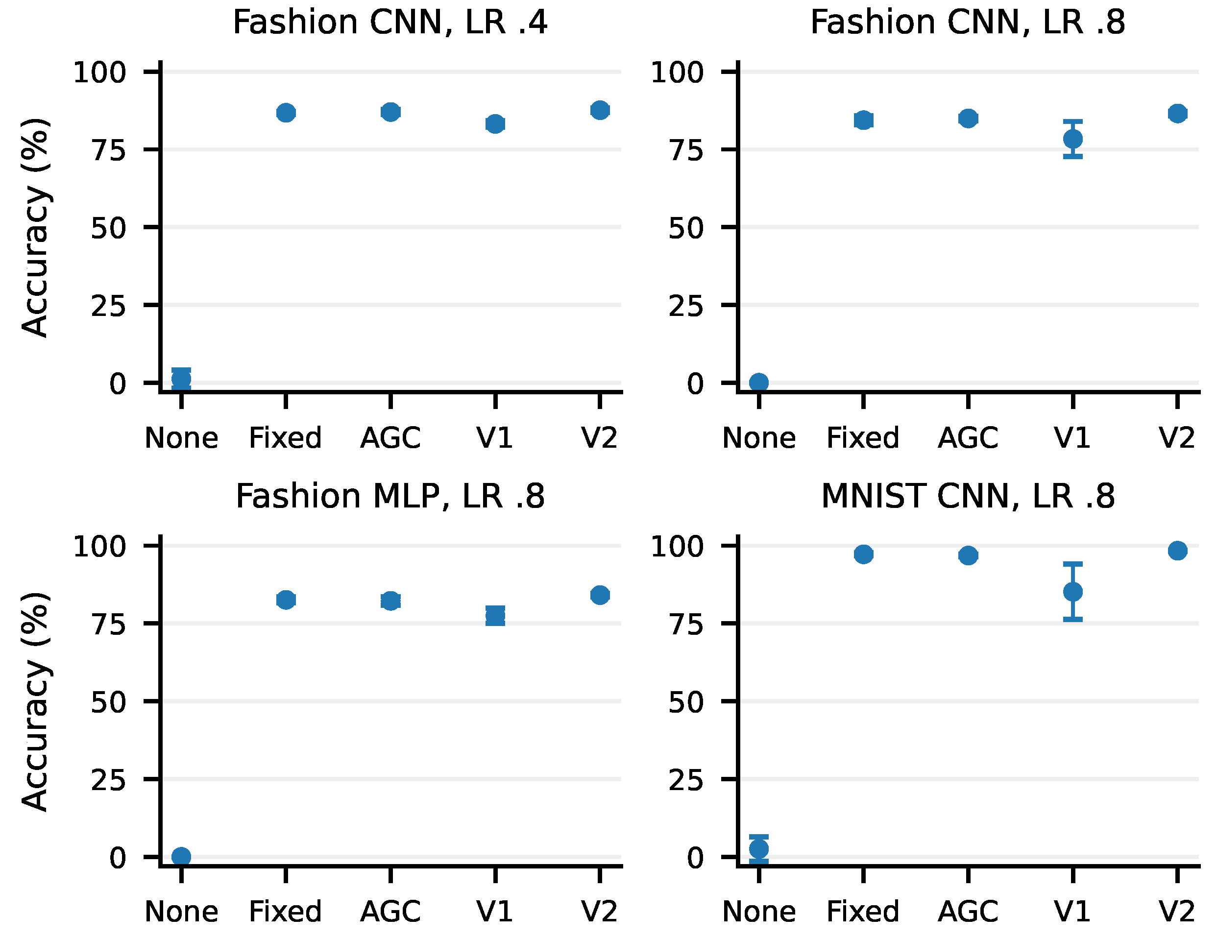
Figure A2.
Earlier mechanism controls, eight paired seeds. The intensity-matched fixed comparator was selected by calibration clipping intensity, whereas the new fixed baseline was selected by validation accuracy. The earlier paired intervals do not establish an incremental alignment or online-feedback benefit over replay. Zero gain retains moving bounds.
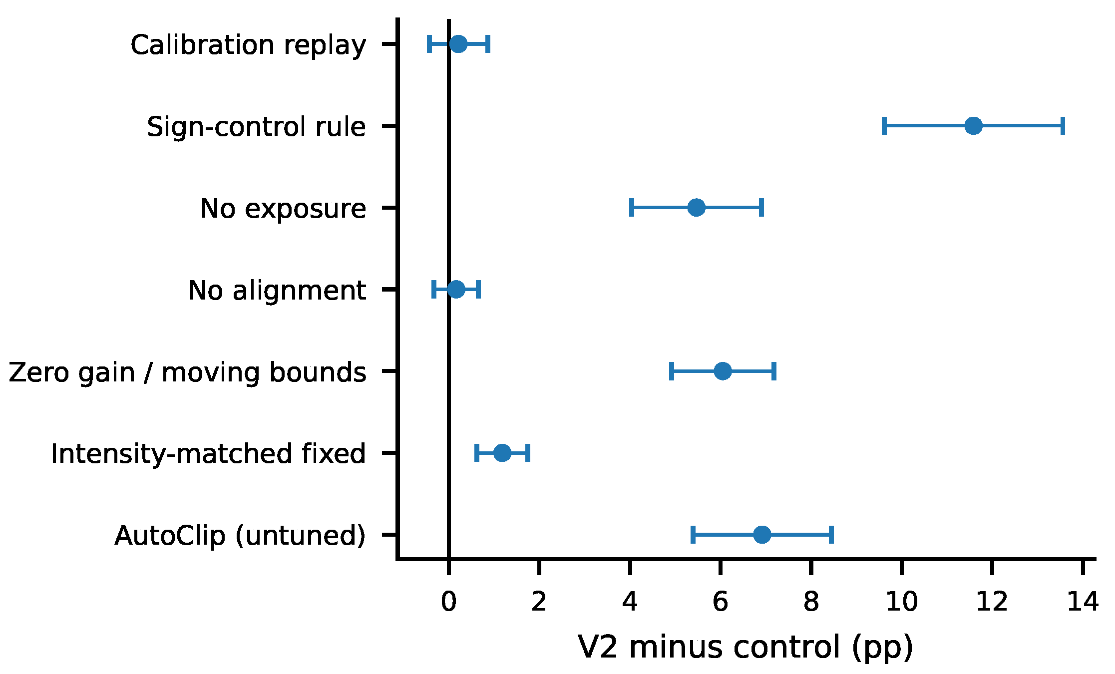
Figure A3.
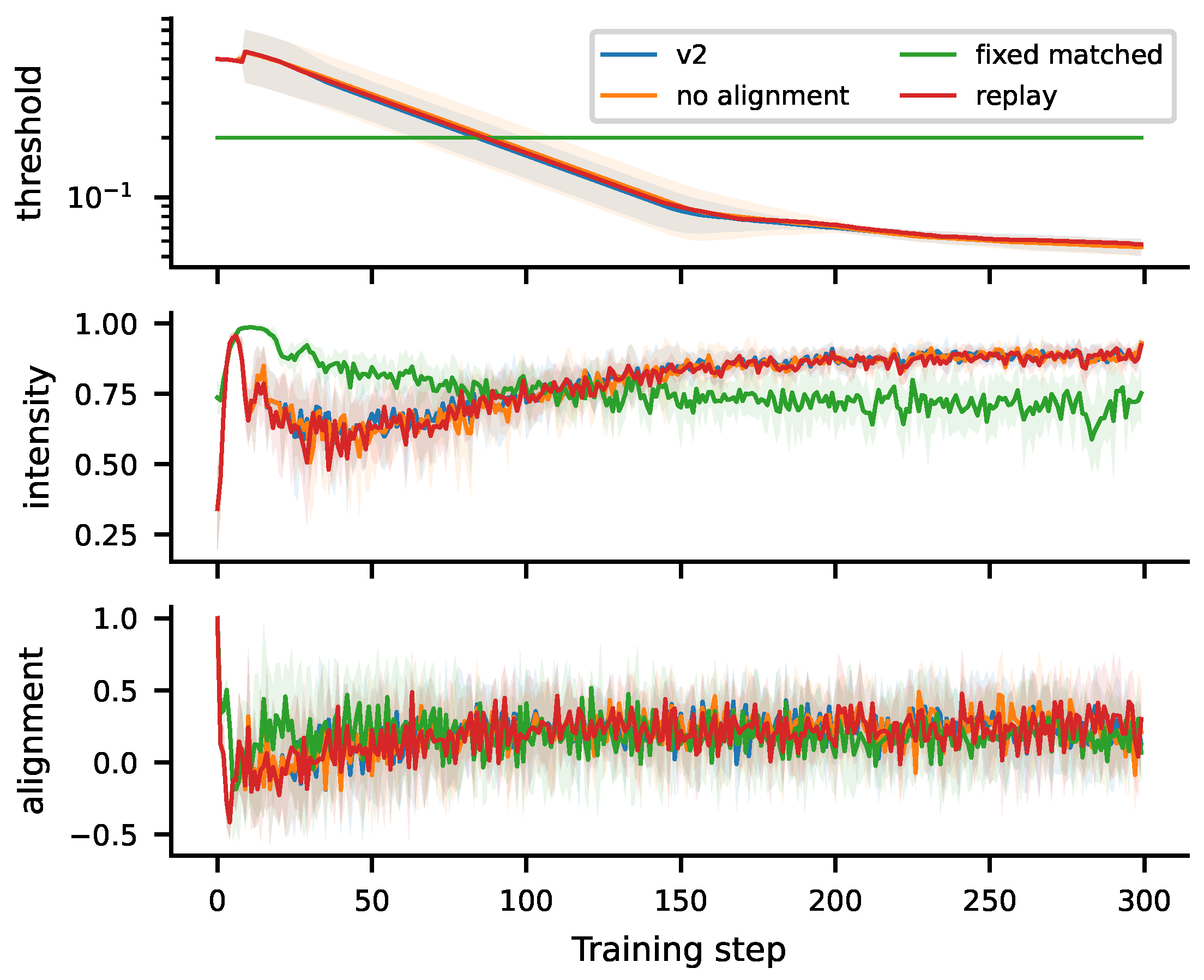
Earlier V2 mechanism trajectories: applied threshold, clipping intensity and gradient alignment, aggregated over eight paired seeds. Bands show across-seed standard deviation, not confidence intervals. The curves illustrate threshold profiles and controller activity; similarity or apparent reversal alone does not establish predictive information or causal accuracy benefit. Compare with the completed confirmation trajectories in Figure 2, where lower-bound occupancy and alignment masking are supported by a separate full-trace audit.
Together, these historical plots explain the progression from promising small-subset observations to a stronger comparison with tuned clipping and calibration replay. The confirmation results constrain the original mechanism interpretation rather than invalidate the recorded exploratory measurements. Neither campaign proves that modifying only the lower bound would improve accuracy; that intervention has not been tested here.
Appendix D. Completed Screening Protocol and Negative Gate
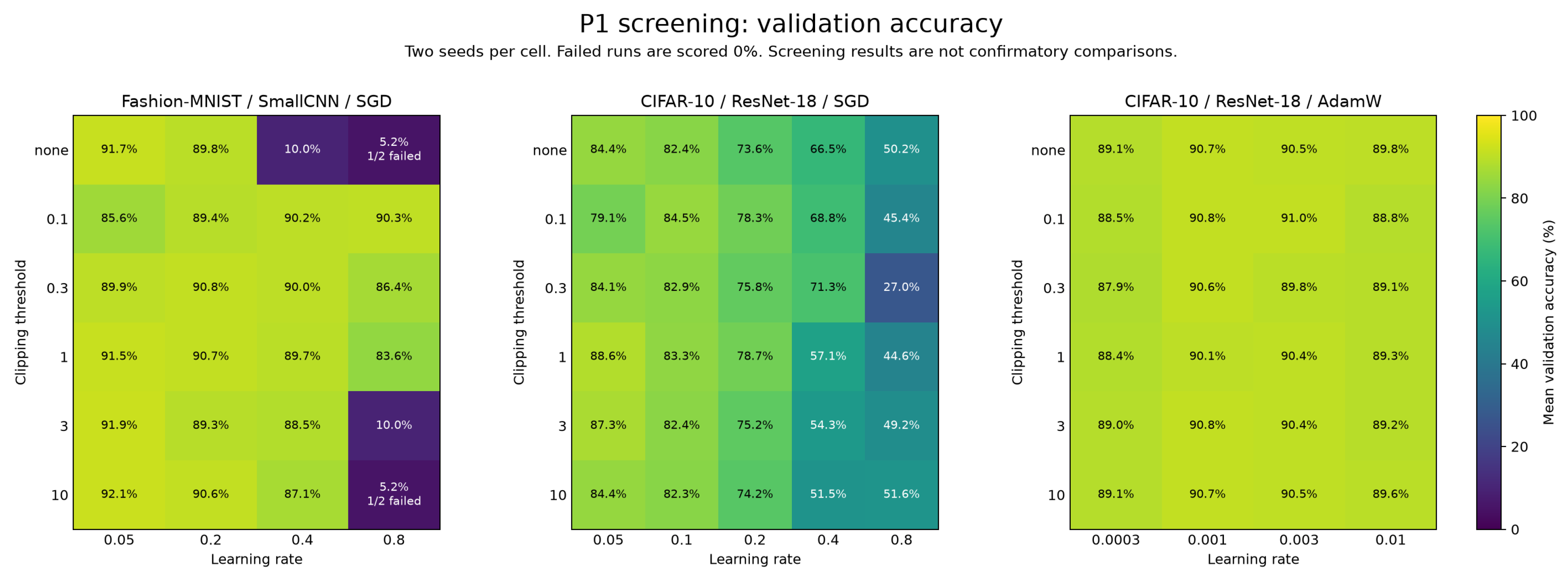
This separate screening campaign must not be pooled with the ResNet-20 confirmation study. It used ResNet-18 for CIFAR-10, two screening seeds, 20 epochs, and validation evaluation. Training/validation sizes were 55,000/5,000 for FashionMNIST and 45,000/5,000 for CIFAR-10, split seed 1729. The SGD learning-rate grids were for FashionMNIST and for CIFAR-10; the AdamW grid was . Each learning rate included no clipping and fixed thresholds .
Table A7.
Completed screening outcomes. These are validation screening runs, not independent confirmation of DAGC. Adverse events are counts across runs.
Table A7.
Completed screening outcomes. These are validation screening runs, not independent confirmation of DAGC. Adverse events are counts across runs.
| Family | Runs | Full budget | Early stops | Adverse events |
|---|---|---|---|---|
| FashionMNIST / SmallCNN / SGD | 48 | 46 | 2 | 14 |
| CIFAR-10 / ResNet-18 / SGD | 60 | 60 | 0 | 0 |
| CIFAR-10 / ResNet-18 / AdamW | 48 | 48 | 0 | 0 |
The frozen adverse-event label included a loss spike after step 50 above , nonfinite loss/gradient/update, or loss above 100. Future labels covered steps 1–20; unknown negative tails were censored and observed terminal positives were retained. Labels were constructed before every-fifth-step subsampling. Base predictors included progress, learning rate, loss and its slope, gradient/update norms, alignment, and optimizer-state proxies. Added history features were exposure EMA, duty cycle, switching rate, burst age, time since transition, and intensity. Grouped evaluation held out seeds, complete configurations, or families; individual steps were never randomly split across training and evaluation.
G1 required at least ten informative runs in every grouped analysis, a mean AUPRC increment of at least 0.01, a bootstrap lower bound above zero, and positive mean increments in all three families. Only two runs were evaluable: FashionMNIST, LR 0.8, fixed threshold 3, seeds 0 and 1. The exploratory seed-held-out interval was ; the configuration-held-out interval was . Neither can justify population-wide inference with two screening seeds. Withholding FashionMNIST left no positive training labels; withholding either CIFAR family left no positive evaluation labels, preventing the required family-held-out comparison.
Event-count robustness used on/off margins and dwell values . For runs with median count at least two, the relative range had to be at most 0.5. Only 27/63 met this criterion; the campaign required at least 75%. Thresholds and labels were not revised retrospectively to make the gate pass.
The two early stops were FashionMNIST at LR 0.8, seed 0: no clipping stopped after 10 steps (loss 2605.40), and threshold 10 after 12 steps (loss 160.40). Their outcomes remain in the screening map at zero accuracy. Runs with finite chance-level accuracy retain their observed values. There were no process errors; maintenance interruptions were not counted as scientific failures.
Figure A4.
Complete validation screening map, averaged over two seeds per configuration; instability stops contribute zero accuracy. The map describes screening behavior and does not replace paired confirmation.
Figure A4.
Complete validation screening map, averaged over two seeds per configuration; instability stops contribute zero accuracy. The map describes screening behavior and does not replace paired confirmation.
The accompanying evidence/ directory contains all 156 run summaries, the G1 report, the verification record, and the frozen screening protocol. The screening source is develop/lyx commit bbc9214. The separate confirmation study was completed in develop/lyx1 commit ede9c4d: all 117 calibration and 288 confirmation outcomes are included in the compact audited export at results/lyx1/evidence/. The completed confirmation results and historical screening are integrated on develop/yzs. The screening G1 failure remains a result of that separate campaign and does not imply that confirmation is still pending. Code and public records are available at https://github.com/alexsongyzs-dotcom/Dynamics_Aware_Gradient_Clipping/tree/develop/yzs.
Appendix E. Original V1 Benchmarks and Additional Exploratory Figures
The initial A3 and A4 studies used V1 with initial threshold 1.0; they must not be presented as V2 evaluations. A3 has five seeds per variant and A4 has five seeds per policy in each of eight dataset/model/optimizer settings. V1 does not uniformly outperform the no-clipping baseline. Their raw tables lack explicit failure flags, so the figures report the recorded scores rather than asserting that all runs were failure-free. Historical normal-approximation error bars are replaced here with Student-t intervals. Complete audit records and source hashes accompany this manuscript in audit_20261010/.
Figure A5.
Original V1 ablations, five seeds per variant. Zero gain retains moving bounds; it is distinct from fixed global clipping.
Figure A5.
Original V1 ablations, five seeds per variant. Zero gain retains moving bounds; it is distinct from fixed global clipping.
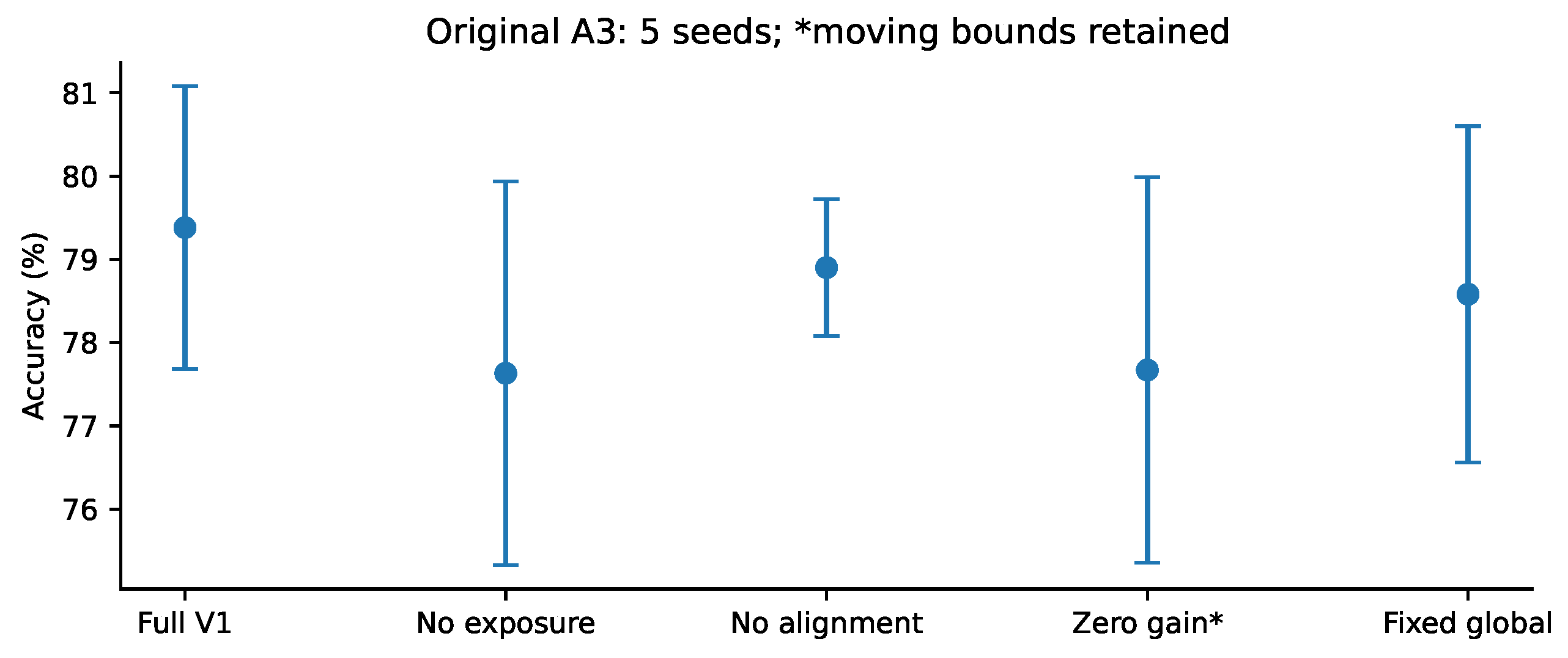
Figure A6.
All eight original A4 settings, five seeds per policy. Error bars are Student-t 95% intervals and scores are exploratory.
Figure A6.
All eight original A4 settings, five seeds per policy. Error bars are Student-t 95% intervals and scores are exploratory.
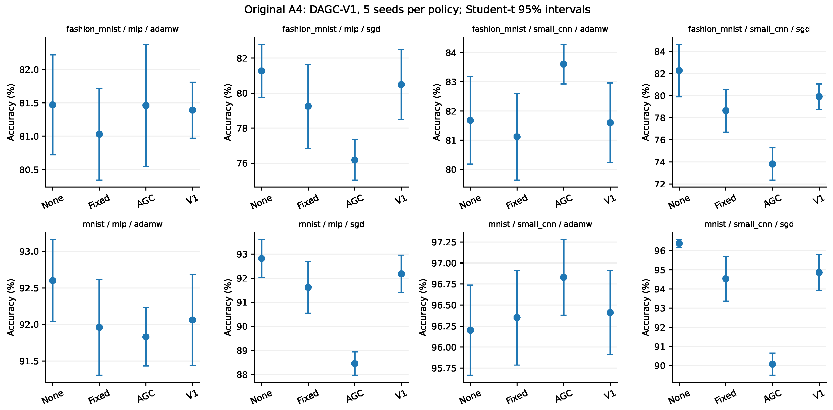
Figure A7.
Development reference sweep stratified by controller gain. Each point has three seeds; gains are not pooled. Realized exposure differs from the reference and cannot be interpreted as target-rate tracking.
Figure A7.
Development reference sweep stratified by controller gain. Each point has three seeds; gains are not pooled. Realized exposure differs from the reference and cannot be interpreted as target-rate tracking.
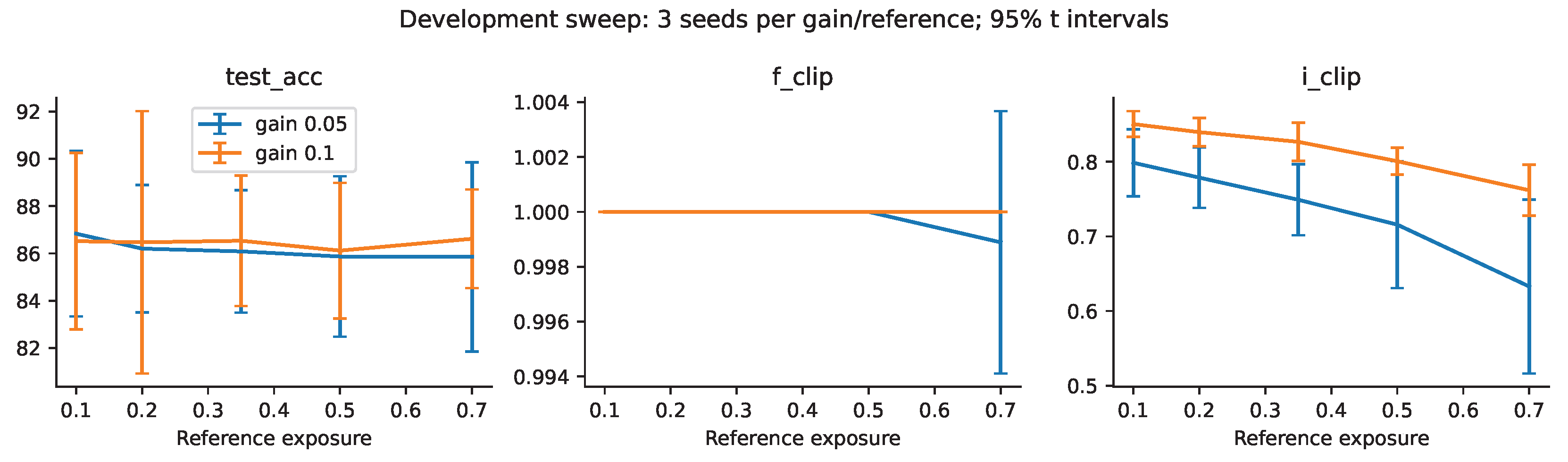
Figure A8.
Exploratory learning-rate perturbations, eight paired seeds. V2-minus-replay intervals span zero; nonsignificance is not equivalence.
Figure A8.
Exploratory learning-rate perturbations, eight paired seeds. V2-minus-replay intervals span zero; nonsignificance is not equivalence.
Single-seed smoke runs and high-learning-rate pilot selection are retained as development artifacts, not replication evidence. The unstable-band tables include legacy comparator implementations whose fidelity has not been verified; they are not used to establish superiority over published ZClip or AdaGC.
Appendix F. Mathematical Mechanism: Exact Results and Their Limits
This appendix separates implementation-level facts from conditional statements about the value of feedback. None establishes unconditional test-accuracy superiority of DAGC or its alignment term. In particular, a theorem about an optimal feedback policy is not a theorem that DAGC realizes that policy.
Appendix F.1. Exposure Feedback with Exponential Smoothing
Use the stationary, exogenous norm distribution of Section 3, with inactive bounds and no alignment term. Define and . The deterministic mean-field recursion is
Proposition A1.
Suppose , , and an interior fixed point satisfies and . The mean-field fixed point is linearly unstable.
Proof.
Write and . For the state , the Jacobian at the fixed point is
Its characteristic polynomial is . Since and as , it has a real root greater than one. □
The positive eigenvalue exceeding one proves local instability of this mean-field equilibrium only. Moving bounds, alignment, and the evolving training distribution are excluded assumptions, not small perturbations whose effects have been proved negligible.
Appendix F.2. What the Direction Penalty Provably Changes
Proposition A2
(One-step monotonicity and saturation). Compare two controller updates from the same state , with the same positive bounds , gains , , and reference signal . Let
Then
They are equal when , or when both proposals saturate at the same bound. If and both proposals lie strictly inside the bounds, .
Proof.
In log coordinates, projection is the monotone, 1-Lipschitz map . The unprojected difference is . Monotonicity and the derivative bound place it in ; applying P preserves order and cannot increase the difference. Strictness holds without projection saturation because tanh is strictly increasing. □
This result concerns the next threshold at a shared state. It does not order the full trajectories after the two policies change their gradients, exposures, and bounds. A negative instantaneous alignment is also not sufficient for activation: the implemented penalty uses the smoothed state A.
Proposition A3
(Inactive direction term gives identical training). Start full DAGC and its no-alignment variant with identical model, optimizer, controller, and random-stream states. If the full run has at every controller update, their thresholds, model states, and losses are identical at every step.
Proof.
At the initial shared state the direction penalty is zero. Both policies use the same current threshold and sample, hence the same raw and clipped gradients. Their exposure, norm history, moving bounds, and optimizer updates are identical, giving the same next state. Induction repeats this argument; the hypothesis makes the full policy’s direction penalty zero at each step. □
Thus no strictly positive directional benefit can hold uniformly over all training problems. Merely observing a nonzero penalty establishes intervention, not improved loss or generalization.
Appendix F.3. Exact Replay Equivalence and Its Scope
Proposition A4
(Replay of a run’s own applied thresholds). Consider any deterministic execution conditional on its initial state and complete random stream, including minibatches and augmentation. Save the thresholds actually applied by a feedback run. A replay run using that exact step-indexed trace, the same initial model/optimizer state, and the same random stream has identical raw gradients, clipped gradients, optimizer states, parameters, and evaluations at all steps.
Proof.
At step zero both executions have the same parameters and training sample, so their raw gradients agree. The replayed applied threshold makes clipping identical. The deterministic optimizer update, including coupled weight decay and momentum, then produces identical next states. Repeat by induction. The replay need not reconstruct controller states; it only reproduces its applied thresholds, and its diagnostics must not alter the training random stream. □
This oracle trace comes from the very run being reproduced and is not our independent-calibration comparator. The proposition therefore neither proves nor disproves a benefit over calibration-trace replay. It does prove that a successful feedback trajectory can be reproduced by a schedule when the schedule contains the same realized decisions. In a problem where feedback produces the same trace for every seed, independent replay is also identical; universal strict dominance of feedback over replay is consequently impossible. Replay still responds to the current gradient norm through its clipping coefficient; it is not a fixed learning-rate multiplier.
Appendix F.4. When Pre-Gradient Information Can Strictly Help
We now give a sufficient-condition analysis that respects causal threshold selection. It compares policies at a common random checkpoint, not policies whose earlier training has already produced different states. Let the objective be , . Let v denote the previous momentum buffer, , and the shared step size. Set weight decay to zero in this model. A policy chooses a threshold c from , , using information available before the next stochastic gradient G is drawn. Assume almost surely, so every admissible policy actively clips. Write , and suppose all second moments needed below are finite. Then the actual momentum update is
Define the scalar conditional prediction
The random state and the future gradient have the same joint distribution for every policy in this one-step comparison. Policies may change c, but may not change that checkpoint distribution or use the future G to choose it.
Proposition A5
(Optimal causal threshold and approximation cost). In this model the optimal -measurable threshold is . If almost surely, any admissible feedback rule satisfies
Without the interior assumption, the difference is at least .
Proof.
Expanding the squared norm gives
Take conditional expectations and use measurability of c. The terms depending on the chosen threshold become . Pointwise minimization over yields projection. In the interior the optimal squared term vanishes, proving Eq. (A9). For a projected optimum, the projection inequality yields the stated lower bound after expanding the difference of squares. □
Proposition A6
(Exact benefit over a predetermined threshold). Under the interior assumptions above, the best constant threshold at that step is . Its advantage relative to any admissible causal rule is exactly
Hence the feedback rule strictly improves expected one-step loss if and only if its squared approximation error is smaller than .
Proof.
A constant policy minimizes at , which is admissible because almost surely. Its minimum value is . Subtract the two risks using Eq. (A9). □
A calibration-generated replay value is constant across new runs at a fixed step, conditional on the independent calibration archive. The result applies to such a common-state, one-step comparison if its other assumptions hold. It does not apply directly to complete DAGC/replay runs with different states, moving bounds, or intermittently inactive clipping.
Appendix F.5. Exact Value of Additional Directional Information
Proposition A7
(Information gain versus policy error). Let be two pre-gradient information sets; the latter may add stored alignment history. Define by Eq. (A8) using , and assume almost surely for . The difference between the optimal policies is
For actual policies measurable with respect to their respective information sets, the exact difference is
Proof.
The tower property gives . Since and are -measurable, . Thus . Use the expanded risk conditional on and subtract the two policies. Taking proves Eq. (A12). □
Additional alignment information helps the ideal policy strictly only if it changes the conditional prediction on a set of positive probability. Even then a particular direction penalty can lose that benefit through policy approximation error. Its sign and coefficient cannot be justified by the mere availability of directional information.
Appendix F.6. Why Threshold Tightening Alone Is Not a Proof of Improvement
Set , , , . Both and actively clip. At , their next losses are 0.4232 and 0.4608: tightening increases loss by 0.0376. At , losses are 0.98 and 0.02: tightening decreases loss by 0.96. A negative stored alignment does not identify which step-size regime holds. These one-step examples refute universal benefit from tightening; they are not complete DAGC training trajectories.
What remains unproved for DAGC.
DAGC has not been shown to predict accurately enough, to obtain incremental information from alignment, or to satisfy this model’s assumptions throughout training. G1 estimates a different risk target. Consequently, these conditional proofs explain when feedback can help; they do not establish DAGC’s empirical incremental benefit or generalization. Paired replay, median, no-alignment, and bound-only controls remain needed.
References
- Pascanu, R.; Mikolov, T.; Bengio, Y. On the difficulty of training recurrent neural networks. In Proceedings of the International Conference on Machine Learning, 2013; pp. 1310–1318. [Google Scholar]
- Seetharaman, P.; Wichern, G.; Pardo, B.; Le Roux, J. AutoClip: Adaptive Gradient Clipping for Source Separation Networks. In Proceedings of the IEEE Workshop on Machine Learning for Signal Processing, 2020. [Google Scholar]
- Brock, A.; De, S.; Smith, S.L.; Simonyan, K. High-Performance Large-Scale Image Recognition Without Normalization. In Proceedings of the International Conference on Machine Learning, 2021. [Google Scholar]
- Zhang, J.; Karimireddy, S.P.; Veit, A.; Kim, S.; Reddi, S.; Kumar, S.; Sra, S. Gradient Clipping and Normalization for Nonconvex Optimization. In Proceedings of the International Conference on Machine Learning, 2020. [Google Scholar]
- Kumar, A.; Owen, L.; Roy Chowdhury, N.; Güra, F. ZClip: Adaptive Spike Mitigation for LLM Pre-Training. arXiv 2025, arXiv:2504.02507. [Google Scholar]
- Wang, G.; Li, S.; Chen, C.; Zeng, J.; Yang, J.; Sun, T.; Ma, Y.; Yu, D.; Shen, L. AdaGC: Improving Training Stability for Large Language Model Pretraining. arXiv 2025, arXiv:2502.11034. [Google Scholar]
- Li, Z.; Wu, Y.; Chang, Y. AGGC: Adaptive Group Gradient Clipping for Stabilizing Large Language Model Training. arXiv 2026, arXiv:2601.11864. [Google Scholar]
- Tang, J.; Drori, Y.; Chang, D.; Sathiamoorthy, M.; Gilmer, J.; Wei, L.; Yi, X.; Hong, L.; Chi, E.H. Improving Training Stability for Multitask Ranking Models in Recommender Systems. In Proceedings of the Proceedings of the 29th ACM SIGKDD Conference on Knowledge Discovery and Data Mining, 2023. [Google Scholar]
- Wortsman, M.; Dettmers, T.; Zettlemoyer, L.; Morcos, A.; Farhadi, A.; Schmidt, L. Stable and Low-Precision Training for Large-Scale Vision-Language Models. In Proceedings of the Advances in Neural Information Processing Systems, 2023. [Google Scholar]
- Andrew, G.; Thakkar, O.; McMahan, H.B.; Ramaswamy, S. Differentially Private Learning with Adaptive Clipping. In Proceedings of the Advances in Neural Information Processing Systems, 2021; Vol. 34. [Google Scholar]
- Merad, I.; Gaïffas, S. Robust Stochastic Optimization via Gradient Quantile Clipping. Transactions on Machine Learning Research, 2024. [Google Scholar]
- Shulgin, E.; Richtárik, P. On the Convergence of DP-SGD with Adaptive Clipping. arXiv 2024, arXiv:2412.19916. [Google Scholar]
- Chen, X.; Wu, Z.S.; Hong, M. Understanding Gradient Clipping in Private SGD: A Geometric Perspective. In Proceedings of the Advances in Neural Information Processing Systems, 2020. [Google Scholar]
- Schaipp, F.; Garrigos, G.; Simsekli, U.; Gower, R. Tracking the Median of Gradients with a Stochastic Proximal Point Method. Transactions on Machine Learning Research, 2025. [Google Scholar]
- Zhang, J.; He, T.; Sra, S.; Jadbabaie, A. Why Gradient Clipping Accelerates Training: A Theoretical Justification for Adaptivity. In Proceedings of the International Conference on Learning Representations, 2020. [Google Scholar]
- Zhang, B.; Jin, J.; Fang, C.; Wang, L. Improved Analysis of Clipping Algorithms for Non-convex Optimization. In Proceedings of the Advances in Neural Information Processing Systems, 2020. [Google Scholar]
- Mai, V.V.; Johansson, M. Stability and Convergence of Stochastic Gradient Clipping: Beyond Lipschitz Continuity and Smoothness. In Proceedings of the International Conference on Machine Learning, 2021. [Google Scholar]
- Koloskova, A.; Hendrikx, H.; Stich, S.U. Revisiting Gradient Clipping: Stochastic Bias and Tight Convergence Guarantees. In Proceedings of the International Conference on Machine Learning, 2023. [Google Scholar]
- Şimşekli, U.; Sagun, L.; Gürbüzbalaban, M. A Tail-Index Analysis of Stochastic Gradient Noise in Deep Neural Networks. In Proceedings of the International Conference on Machine Learning, 2019. [Google Scholar]
- Gorbunov, E.; Danilova, M.; Gasnikov, A. Stochastic Optimization with Heavy-Tailed Noise via Accelerated Gradient Clipping. In Proceedings of the Advances in Neural Information Processing Systems, 2020. [Google Scholar]
- Cutkosky, A.; Mehta, H. High-probability Bounds for Non-Convex Stochastic Optimization with Heavy Tails. arXiv 2021, arXiv:2106.14343. [Google Scholar]
- Sun, T.; Liu, X.; Yuan, K. Revisiting Gradient Normalization and Clipping for Nonconvex SGD under Heavy-Tailed Noise: Necessity, Sufficiency, and Acceleration. J. Mach. Learn. Res. 2025. [Google Scholar] [CrossRef]
- Duchi, J.; Hazan, E.; Singer, Y. Adaptive Subgradient Methods for Online Learning and Stochastic Optimization. J. Mach. Learn. Res. 2011. [Google Scholar] [CrossRef]
- Ward, R.; Wu, X.; Bottou, L. AdaGrad Stepsizes: Sharp Convergence Over Nonconvex Landscapes. In Proceedings of the International Conference on Machine Learning, 2019. [Google Scholar]
- Kingma, D.P.; Ba, J. Adam: A Method for Stochastic Optimization. In Proceedings of the International Conference on Learning Representations, 2015. [Google Scholar]
- Loshchilov, I.; Hutter, F. Decoupled Weight Decay Regularization. In Proceedings of the International Conference on Learning Representations, 2019. [Google Scholar]
- You, Y.; Li, J.; Reddi, S.; Hseu, J.; Kumar, S.; Bhojanapalli, S.; Song, X.; Demmel, J.; Keutzer, K.; Hsieh, C.J. Large Batch Optimization for Deep Learning: Training BERT in 76 Minutes. In Proceedings of the International Conference on Learning Representations, 2020. [Google Scholar]
- Glorot, X.; Bengio, Y. Understanding the Difficulty of Training Deep Feedforward Neural Networks. In Proceedings of the Proceedings of the Thirteenth International Conference on Artificial Intelligence and Statistics, 2010; pp. 249–256. [Google Scholar]
- Sutskever, I.; Martens, J.; Dahl, G.; Hinton, G. On the Importance of Initialization and Momentum in Deep Learning. In Proceedings of the International Conference on Machine Learning, 2013; pp. 1139–1147. [Google Scholar]
- Ioffe, S.; Szegedy, C. Batch Normalization: Accelerating Deep Network Training by Reducing Internal Covariate Shift. In Proceedings of the International Conference on Machine Learning, 2015; pp. 448–456. [Google Scholar]
- Santurkar, S.; Tsipras, D.; Ilyas, A.; Madry, A. How Does Batch Normalization Help Optimization? In Proceedings of the Advances in Neural Information Processing Systems, 2018. [Google Scholar]
- He, K.; Zhang, X.; Ren, S.; Sun, J. Deep Residual Learning for Image Recognition. In Proceedings of the Proceedings of the IEEE Conference on Computer Vision and Pattern Recognition, 2016; pp. 770–778. [Google Scholar]
- Wortsman, M.; Liu, P.J.; Xiao, L.; Everett, K.; Alemi, A.; Adlam, B.; Co-Reyes, J.D.; Gur, I.; Kumar, A.; Novak, R.; et al. Small-scale Proxies for Large-scale Transformer Training Instabilities. In Proceedings of the International Conference on Learning Representations, 2024. [Google Scholar]
- Bouthillier, X.; Delaunay, P.; Bronzi, M.; Trofimov, A.; Nichyporuk, B.; Szeto, J.; Sepah, N.; Raff, E.; Madan, K.; Voleti, V.; et al. Accounting for Variance in Machine Learning Benchmarks. Proc. Proc. Mach. Learn. Syst. 2021, Vol. 3, 730–743. [Google Scholar]
- Cawley, G.C.; Talbot, N.L.C. On Over-fitting in Model Selection and Subsequent Selection Bias in Performance Evaluation. J. Mach. Learn. Res. 2010. [Google Scholar]
- Bergstra, J.; Bengio, Y. Random Search for Hyper-Parameter Optimization. J. Mach. Learn. Res. 2012. [Google Scholar] [CrossRef]
- Recht, B.; Roelofs, R.; Schmidt, L.; Shankar, V. Do ImageNet Classifiers Generalize to ImageNet? In Proceedings of the International Conference on Machine Learning, 2019. [Google Scholar]
- Dror, R.; Baumer, G.; Shlomov, S.; Reichart, R. The Hitchhiker’s Guide to Testing Statistical Significance in Natural Language Processing. In Proceedings of the Proceedings of the 56th Annual Meeting of the Association for Computational Linguistics, 2018. [Google Scholar]
- Holm, S. A Simple Sequentially Rejective Multiple Test Procedure. Scand. J. Stat. 1979. [Google Scholar]
- Lakens, D. Equivalence Tests: A Practical Primer for t Tests, Correlations, and Meta-Analyses. In Social Psychological and Personality Science; 2017. [Google Scholar]
- Xiao, H.; Rasul, K.; Vollgraf, R. Fashion-MNIST: a Novel Image Dataset for Benchmarking Machine Learning Algorithms. arXiv 2017, arXiv:1708.07747. [Google Scholar]
- Krizhevsky, A. Learning Multiple Layers of Features from Tiny Images. In Technical report; University of Toronto, 2009. [Google Scholar]
Figure 1.
Paired effects of DAGC versus the main controls and the no-alignment variant. Bars show 95% intervals; the shaded region is the prespecified point margin. Equivalence requires a separate 90% interval check.
Figure 1.
Paired effects of DAGC versus the main controls and the no-alignment variant. Bars show 95% intervals; the shaded region is the prespecified point margin. Equivalence requires a separate 90% interval check.
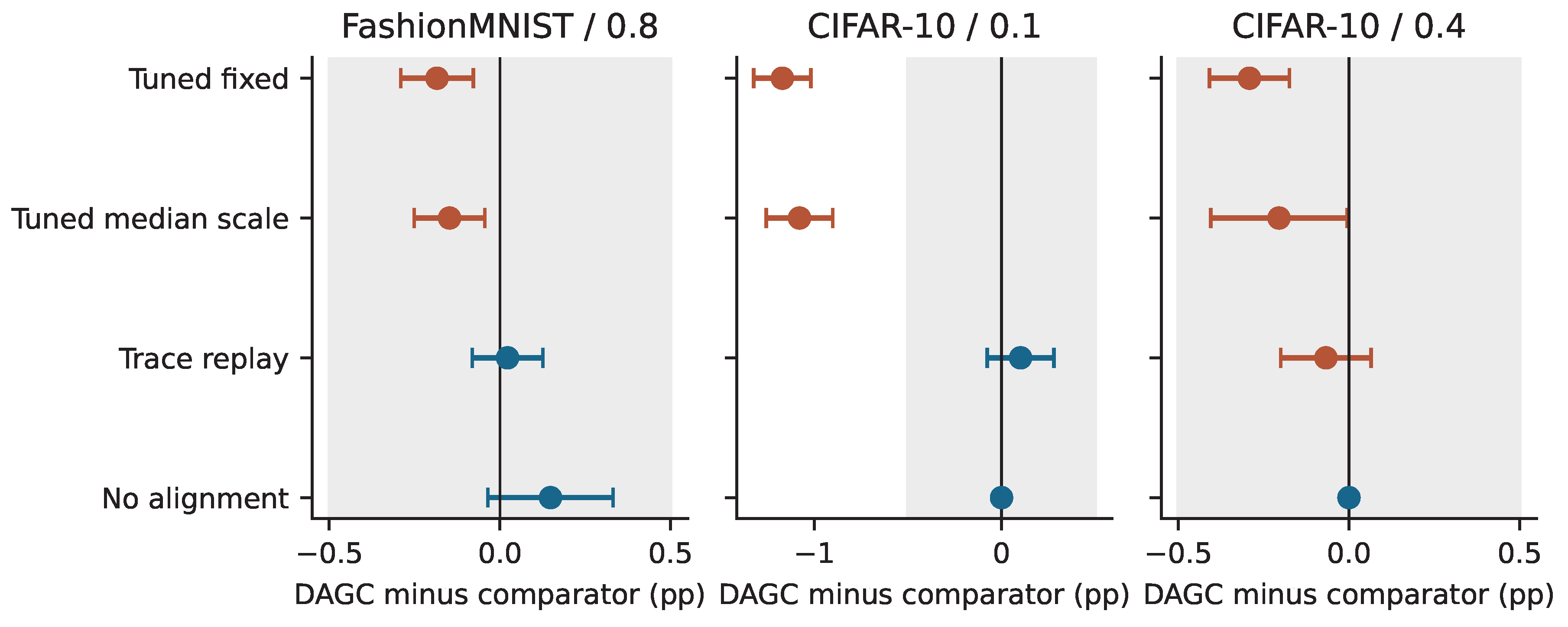
Figure 2.
Applied thresholds and clipping intensities averaged over twelve confirmation seeds and 100 bins of training progress. DAGC and no-alignment curves overlap on CIFAR-10. These observational trajectories describe behavior; they do not establish the causal value of an individual feedback signal.
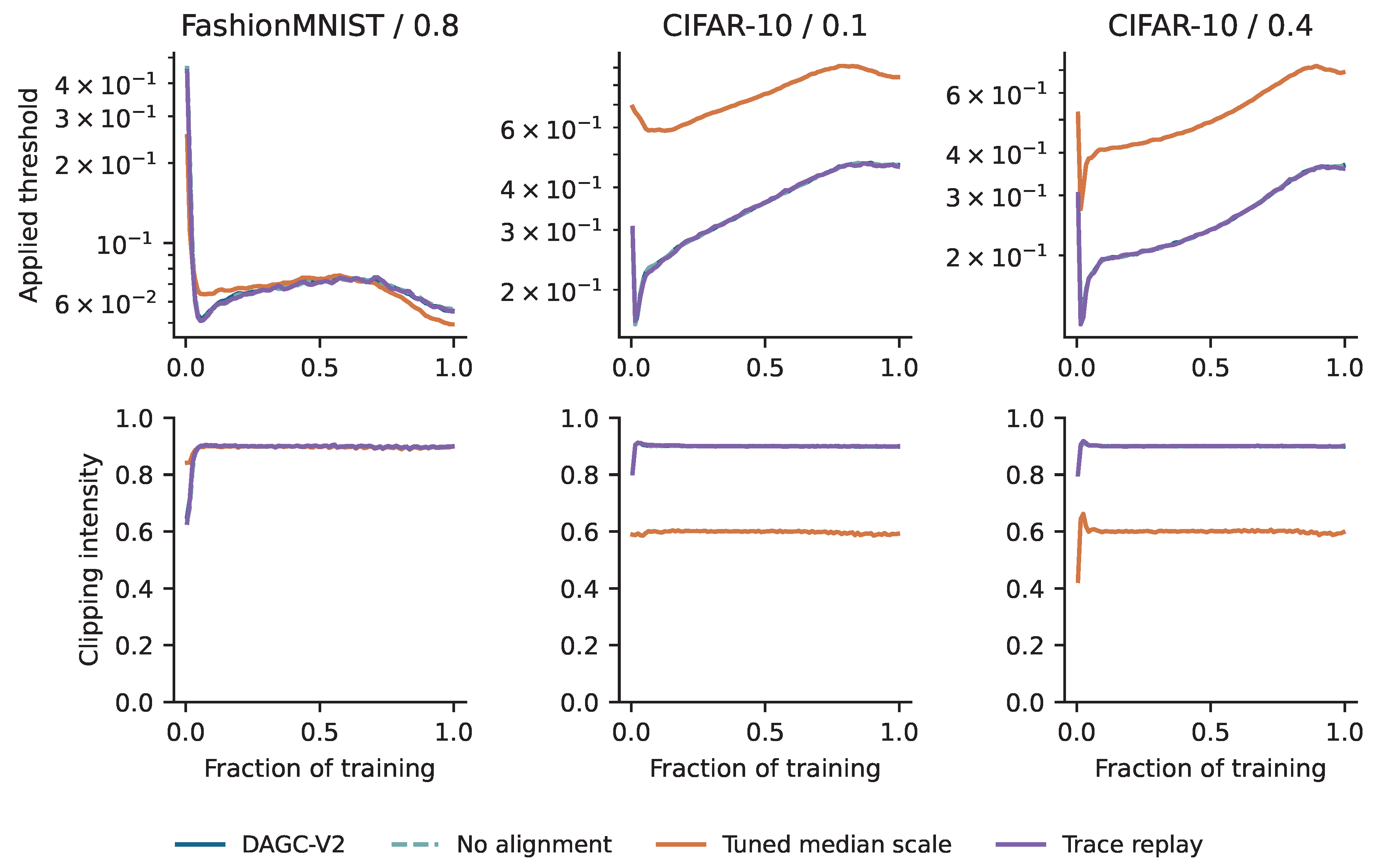
Table 1.
Final test accuracy (percent), mean ± Student-t 95% interval half-width over twelve paired training seeds. Hyperparameters are selected using the validation set. Failures are retained at zero accuracy.
Table 1.
Final test accuracy (percent), mean ± Student-t 95% interval half-width over twelve paired training seeds. Hyperparameters are selected using the validation set. Failures are retained at zero accuracy.
| Policy | FashionMNIST, LR 0.8 | CIFAR-10, LR 0.1 | CIFAR-10, LR 0.4 |
|---|---|---|---|
| No clipping | |||
| Tuned fixed | |||
| Tuned AGC | |||
| Tuned AutoClip | |||
| Tuned median scale | |||
| DAGC-V2 | |||
| No alignment | |||
| Trace replay |
Table 2.
Primary paired comparisons in percentage points: DAGC minus the comparator. Intervals are unadjusted 95% paired t intervals; is the exact two-sided sign-flip p-value after Holm adjustment over all nine tests. Win counts exclude ties.
Table 2.
Primary paired comparisons in percentage points: DAGC minus the comparator. Intervals are unadjusted 95% paired t intervals; is the exact two-sided sign-flip p-value after Holm adjustment over all nine tests. Win counts exclude ties.
| Condition / initial LR | Comparator | Difference | 95% interval | Wins | |
|---|---|---|---|---|---|
| FashionMNIST / 0.8 | Tuned fixed | -0.184 | [-0.291, -0.078] | 1/12 | 0.0176 |
| FashionMNIST / 0.8 | Tuned median scale | -0.148 | [-0.251, -0.044] | 2/12 | 0.0635 |
| FashionMNIST / 0.8 | Trace replay | +0.023 | [-0.081, +0.126] | 5/12 | 0.7236 |
| CIFAR-10 / 0.1 | Tuned fixed | -1.172 | [-1.325, -1.019] | 0/12 | 0.0044 |
| CIFAR-10 / 0.1 | Tuned median scale | -1.080 | [-1.257, -0.903] | 0/12 | 0.0044 |
| CIFAR-10 / 0.1 | Trace replay | +0.102 | [-0.076, +0.280] | 8/12 | 0.7236 |
| CIFAR-10 / 0.4 | Tuned fixed | -0.292 | [-0.409, -0.175] | 1/12 | 0.0103 |
| CIFAR-10 / 0.4 | Tuned median scale | -0.205 | [-0.405, -0.005] | 3/12 | 0.1914 |
| CIFAR-10 / 0.4 | Trace replay | -0.068 | [-0.200, +0.065] | 4/12 | 0.7236 |
Disclaimer/Publisher’s Note: The statements, opinions and data contained in all publications are solely those of the individual author(s) and contributor(s) and not of MDPI and/or the editor(s). MDPI and/or the editor(s) disclaim responsibility for any injury to people or property resulting from any ideas, methods, instructions or products referred to in the content. |
© 2026 by the authors. Licensee MDPI, Basel, Switzerland. This article is an open access article distributed under the terms and conditions of the Creative Commons Attribution (CC BY) license (http://creativecommons.org/licenses/by/4.0/).
Copyright: This open access article is published under a Creative Commons CC BY 4.0 license, which permit the free download, distribution, and reuse, provided that the author and preprint are cited in any reuse.