
Submitted:
10 October 2026
Posted:
13 October 2026
You are already at the latest version
Abstract
Change detection in high-resolution remote sensing imagery is susceptible to adversary effects of within-class spectral heterogeneity, shadows, and complex spatial structures. Meanwhile, change detection methods based on land-cover posterior probabilities generally rely on reliable semantic training information, making complete manual interpretation costly. To address these issues, this study develops a change detection framework that integrates SEEDS-guided SAM object construction and active learning-based interpretation with FCM-CSBN-CVAPS posterior probability inference. First, representative points of SEEDS superpixels are used as prompts for SAM to generate candidate objects and construct a mutually exclusive object partition. Second, based on the spectral statistical features of the superpixels and an XGBoost classifier, active learning is employed to select highly uncertain samples for limited manual annotation, thereby obtaining object-level semantic information. Finally, FCM is used to characterize pixel-level spectral uncertainty, while CSBN incorporates spatial context to estimate posterior probabilities of land-cover classes. Bi-temporal change measurement and changed-area extraction are then performed in the posterior probability space. Experimental results show that the proposed framework achieves stable change detection performance with only approximately 10% manual annotation. On DS1, DS2, and DS3, the Kappa coefficients reach 83.87%, 86.05%, and 90.21%, respectively, while the corresponding F1 scores are 87.62%, 91.78%, and 91.31%, outperforming the compared methods. These results indicate an effective balance between false-alarm suppression and missed-detection control. In adaptive evaluation experiments, the mean Kappa and F1 scores reach 84.73% and 87.88%, respectively, further confirming the effectiveness and stability of the proposed framework across diverse remote sensing scenarios.
Keywords:
Segment Anything Model
; change detection
; active learning
; superpixel segmentation
; fuzzy C-means clustering
1. Introduction
Remote sensing image change detection identifies spatiotemporal changes in land cover and surface-object states by analyzing differences between multitemporal images acquired over the same area. As an important research topic in intelligent remote sensing interpretation, it has been widely applied to territorial spatial monitoring, urban expansion analysis, disaster assessment, and ecological and environmental protection [1]. With the continuous improvement in the spatial resolution of remote sensing imagery, detailed information such as object boundaries, shapes, and spatial structures can be represented more clearly. However, higher spatial resolution also aggravates within-object spectral heterogeneity, intra-class spectral variability, and inter-class spectral similarity, making change detection more susceptible to interference from illumination differences, shadows, noise, and image registration errors. Therefore, how to effectively exploit the spatial structure and semantic information of ground objects in high-resolution imagery under limited annotation conditions, while achieving stable change detection performance, remains an important challenge in this field [2].
To address the aforementioned issues, existing studies on remote sensing image change detection have generally followed two major technical paradigms: traditional analytical methods and deep learning-based methods [3,4,5,6]. Traditional change detection methods typically identify changes based on spectral differences, transformed features, or classification results derived from bi-temporal images. Representative approaches include image differencing, principal component analysis (PCA), post-classification comparison, and change vector analysis (CVA) [7,8,9,10,11,12,13,14]. CVA characterizes change magnitude by calculating the distance between spectral vectors from bi-temporal images and does not require prior interpretation results; however, it is susceptible to radiometric differences and spectral noise. In contrast, post-classification comparison independently interprets the images acquired at each time point and identifies change types by comparing the corresponding interpretation results. Nevertheless, the accumulation of classification errors can directly degrade change detection accuracy. To mitigate error propagation caused by hard classification, related studies have incorporated posterior probabilities of land-cover classes into CVA to characterize differences in land-cover states between bi-temporal images in the probability space [15], thereby enabling change detection to account for uncertainty in class membership. However, such methods generally still require sufficiently reliable and representative semantic information on land-cover classes as prior knowledge or training data. Generating complete land-cover labels for both temporal images entails substantial manual effort and also relies on a certain level of professional interpretation expertise.
On the other hand, to enhance feature representation in complex scenes and further reduce the dependence on large amounts of manually labeled data, deep learning has gradually become an important technical paradigm for remote sensing change detection. Models such as convolutional neural networks, Siamese networks, and Transformers can learn multiscale change features from bi-temporal imagery and have demonstrated strong performance in complex-scene change detection [16,17,18,19,20,21,22]. With the advancement of research, the corresponding learning paradigms have progressively expanded from fully supervised learning toward semi-supervised, weakly supervised, and few-shot learning, aiming to alleviate the practical challenges of high annotation costs and limited labeled samples in high-resolution remote sensing imagery [23]. Unsupervised and semi-supervised methods further reduce the dependence on complete change annotations by exploiting unlabeled data through strategies such as pseudo-labeling, self-training, and consistency regularization [16,20]. Meanwhile, the introduction of foundation models has provided new technical avenues for remote sensing image segmentation and change feature extraction [21]. However, reduced annotation requirements do not necessarily imply that deep learning models can maintain consistent advantages under all application conditions. When only limited labeled samples are available for the target area, when distribution shifts exist between the training data and the actual application scenarios, or when computational resources are constrained, model performance may still be adversely affected [24,25]. In addition, end-to-end binary prediction methods generally focus on the final change map and provide relatively limited explicit representation of pixel-level class uncertainty and its spatial relationships. Therefore, under limited annotation conditions, how to fully exploit the spatial structure of high-resolution imagery while preserving uncertainty information associated with land-cover classes, so as to achieve stable change detection performance, remains worthy of further investigation.
High-resolution remote sensing imagery contains rich information on object shape and spatial adjacency. Analyses conducted solely at the pixel level are prone to producing fragmented regions and isolated noise. To address this issue, superpixel-based and object-based methods have increasingly been applied to change detection. By grouping pixels with similar spectral and spatial characteristics into regional objects, these methods can reduce computational redundancy and improve the spatial consistency of detection results [26,27,28]. However, region partitioning in conventional superpixel-based and object-based methods mainly depends on local spectral similarity, and the segmentation results are also influenced by predefined scale parameters. In scenes with complex boundaries, the resulting segmentation boundaries may still deviate from the true contours of ground objects. With the development of vision foundation models, their general-purpose object segmentation capabilities acquired through large-scale pretraining have provided a new approach for high-quality object extraction from remote sensing imagery. The Segment Anything Model (SAM), as a representative vision foundation model, exhibits strong general-purpose segmentation capabilities and can generate object masks from prompts such as points and bounding boxes, providing a new solution for object extraction from high-resolution remote sensing imagery [29,30,31]. Researchers have introduced SAM into remote sensing change detection, leveraging its general-purpose segmentation capabilities to improve object boundary delineation and the representation of changed regions in complex scenes, and have further explored its integration into image interpretation or change detection frameworks to improve detection accuracy [29,32,33,34,35]. It should be noted that a key strength of SAM lies in its ability to generate relatively complete object masks whose boundaries closely follow object contours; however, these masks are inherently class-agnostic and do not provide explicit semantic labels. Moreover, directly applying SAM to complex remote sensing scenes may result in overlapping masks, inconsistent segmentation scales, over-segmentation, or under-segmentation. Therefore, designing prompting strategies tailored to the spatial characteristics of remote sensing imagery and assigning meaningful land-cover semantics to SAM-generated objects with low annotation costs are critical to effectively leveraging SAM for change detection.
To address the high manual annotation cost associated with object-level semantic acquisition, active learning provides a feasible approach for remote sensing image interpretation with only a limited amount of labeled data. By iteratively selecting the samples that are most uncertain or representative to the classification model for manual annotation, active learning can improve classification performance while maintaining a relatively low annotation cost [36,37,38,39,40]. For high-resolution remote sensing imagery, using superpixels or objects as query units is more consistent with the spatial structure of ground objects than pixel-wise annotation and also helps reduce redundant labeling. Existing studies have incorporated clustering, neighborhood similarity, and deep features into active sample selection. However, most of these efforts have primarily focused on single-temporal image classification or end-to-end change detection, while the synergistic relationships among object generation, few-shot semantic interpretation, and probabilistic change analysis remain insufficiently investigated. Moreover, the superpixel-level semantic results obtained through active learning are not entirely accurate. When local superpixels are misclassified, how to further exploit within-object spatial consistency to constrain such errors and transform limited but effective semantic information into the training information required for subsequent probabilistic change analysis remains insufficiently investigated.
In summary, high-resolution remote sensing image change detection still faces two interrelated challenges. On the one hand, spectral heterogeneity, mixed pixels, and complex spatial structures make pixel-wise change detection prone to false alarms and fragmented errors, necessitating the joint exploitation of object structure, spectral uncertainty, and spatial contextual information. On the other hand, although change detection based on posterior probabilities of land-cover classes can reduce the error propagation caused by directly comparing hard classification results, its performance still depends on effective semantic training information for land-cover classes. Constructing complete land-cover labels for bi-temporal imagery not only incurs substantial manual annotation costs but also relies on professional expertise in remote sensing image interpretation. Existing methods based on superpixel segmentation, SAM, active learning, and posterior probability-based change analysis provide potential solutions from the perspectives of spatial organization, object extraction, low-cost semantic acquisition, and uncertainty-aware change modeling, respectively. However, these techniques have largely been developed independently, and a unified collaborative framework integrating object generation, low-cost semantic acquisition, uncertainty modeling, and probabilistic change discrimination has yet to be established.
To address this issue, this study does not aim to merely replace a specific classifier or change discriminator. Instead, it focuses on the acquisition of reliable semantic priors at low annotation cost and their utilization in probabilistic change detection, and accordingly develops an object-level active interpretation and posterior probability-based change analysis framework. First, the spatial distribution of SEEDS superpixels is used to constrain the point prompts for SAM, and a mutually exclusive object partition covering the entire study area is generated through candidate-mask merging and spatial conflict resolution. Subsequently, superpixels are used as query units in active learning, and object-level land-cover semantics are obtained with only a small amount of manual annotation to provide training information for the subsequent probabilistic model. Finally, FCM is employed to preserve the fuzzy memberships of pixels to different spectral patterns, while CSBN incorporates neighborhood spatial context, and bi-temporal changes are measured in the posterior probability space of land-cover classes. In this way, object-level spatial structure, low-cost manually acquired semantic information, and pixel-level probabilistic change analysis are integrated into a complete processing pipeline.
To address the lack of coordination among the aforementioned components, this study develops an object-level active interpretation and posterior probability-based change analysis framework centered on the acquisition of effective semantic information at low annotation cost and its utilization in posterior probability-based change detection. The framework first exploits the spatial structure of superpixels to assist SAM in generating segmentation masks that cover the entire study area, and then employs active learning to interpret remote sensing imagery with only a small amount of manual annotation. The resulting semantic information is used to support the training of the probabilistic model, thereby bridging the image interpretation stage and the change detection stage. By integrating the spectral fuzziness representation of FCM, the spatial contextual inference of CSBN, and the posterior probability-based change measurement of CVAPS, the proposed framework enables coordinated processing from object-structure construction and low-cost semantic acquisition to pixel-level probabilistic change discrimination.
The main contributions of this study are summarized as follows:
- (1)
- A SEEDS-guided SAM prompting and mask organization method tailored to the object structure of remote sensing imagery is proposed. Representative points within superpixels are used to reduce the mismatch between regular prompting patterns and the spatial structures of ground objects. Overlapping-mask merging, spatial conflict resolution, and uncovered-region handling are further introduced to generate a mutually exclusive object partition covering the entire study area, thereby providing stable spatial units for subsequent object-level semantic interpretation.
- (2)
- An active learning strategy for object-level remote sensing image interpretation is developed. Superpixels are used as the basic query units, and class probabilities are predicted using XGBoost. A breaking-ties strategy is then employed to select highly uncertain samples for manual annotation. Subsequently, area-weighted label aggregation within each object is used to enhance regional semantic consistency, enabling the acquisition of land-cover class information required for subsequent probabilistic change analysis with only limited manual annotation.
- (3)
- A collaborative mechanism is established between object-level semantic interpretation and FCM-CSBN-CVAPS-based probabilistic change detection. Unlike methods that directly compare hard classification results from bi-temporal images, the proposed framework uses land-cover semantics acquired under limited manual supervision as training information for the probabilistic model. FCM is employed to represent spectral fuzziness, CSBN incorporates local spatial context and estimates posterior probabilities of land-cover classes, and CVAPS measures bi-temporal changes in the posterior probability space. In this manner, the direct propagation of local semantic misclassifications from the front-end interpretation stage to the final change map is reduced. Comparative experiments on multiple datasets, parameter sensitivity analysis, multi-scenario adaptability evaluation, and ablation studies demonstrate the effectiveness and stability of the complete framework.
The remainder of this paper is organized as follows. Section 2 presents the overall framework of the proposed method and its constituent modules. Section 3 describes the experimental datasets, experimental settings, and evaluation metrics, and reports comparative experiments, sensitivity analyses, adaptability experiments, and ablation studies. Section 4 discusses the applicability and limitations of the proposed method. Finally, Section 5 summarizes the main findings and outlines directions for future research.
2. Materials and Methods
This study proposes a change detection framework for limited-annotation scenarios, with FCM-CSBN-CVAPS serving as the back-end probabilistic change detection module. By integrating object-level spatial constraints and active semantic acquisition, the framework provides low-cost semantic priors for probabilistic modeling and links object-level semantic interpretation with posterior probability-based change analysis, thereby reducing the reliance on large-scale manual annotation and expert knowledge. The following sections present the overall framework, the individual methodological components, the experimental datasets, the comparison methods, and the evaluation metrics.
2.1. Problem Definition and Overall Framework
Let the bi-temporal remote sensing images after geometric registration and necessary radiometric preprocessing be denoted as:
where H, W, and Bdenote the image height, width, and number of spectral bands, respectively. The two temporal images adopt a unified land-cover class system:
where K denotes the number of land-cover classes. The objective of change detection is to generate a binary change map from the bi-temporal images:
where Ci,j = 1indicates that the land-cover state at location (i,j) has changed, whereas Ci,j = 0 indicates that no change has occurred at that location.
I(1),I(2) ∈ RH×W×B
= {L1,…,Lj,…LK}
C ∈ {0,1}H×W
The overall workflow of the proposed method is illustrated in Figure 1 and consists of two stages: object-level image interpretation and posterior probability-based change detection. In the object-level image interpretation stage, the remote sensing images from the two time points are processed separately. First, the SEEDS algorithm is employed to generate spatially contiguous superpixels with relatively homogeneous internal spectral characteristics. Representative points within each superpixel are then used as point prompts for SAM to obtain candidate ground-object masks. Second, duplicate-mask merging, spatial conflict resolution, and uncovered-region filling are performed on the candidate masks to generate a mutually exclusive object partition covering the entire study area. Subsequently, superpixel-level spectral features are used as input to an XGBoost classifier, and a breaking-ties active query strategy is adopted to iteratively select highly uncertain samples for manual annotation. Finally, area-weighted voting is applied to obtain object-level land-cover interpretation results.
In the change detection stage, fuzzy C-means clustering is first employed to represent the spectral features of each pixel as fuzzy membership degrees to multiple signal classes. Next, based on the object-level image interpretation results, the conditional probabilities between signal-class pairs and land-cover classes are learned. A context-sensitive Bayesian network is then used to integrate the fuzzy memberships of the target pixel and its neighboring pixels, thereby estimating, for each temporal image, the posterior probability that each pixel belongs to each land-cover class. Finally, the bi-temporal change magnitude is calculated in the posterior probability space of land-cover classes, and the final binary change map is obtained using Otsu’s automatic thresholding method.
2.2. SEEDS-Guided SAM-Based Object Segmentation
2.2.1. SEEDS Superpixel Generation and Prompt Point Construction
High-spatial-resolution remote sensing imagery contains rich information on object boundaries, shapes, and spatial adjacency. However, within-object spectral heterogeneity, shadows, and material differences can easily lead to fragmented pixel-wise interpretation results. Superpixels group spatially adjacent pixels with similar spectral characteristics into regional units, thereby reducing the number of processing units and improving the spatial consistency of image interpretation.
SEEDS [41,42] is an energy optimization-based superpixel segmentation algorithm that improves feature homogeneity within superpixels by iteratively adjusting boundary pixels between adjacent superpixels. Compared with regular grids, the boundaries of SEEDS-generated superpixels tend to better conform to locally salient edges in the image, thereby providing relatively stable regional structural information for the generation of SAM point prompts.
Figure 2.
Schematic illustration of SEEDS-guided SAM segmentation.
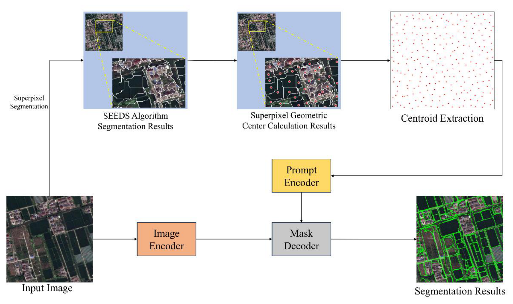
For the image I(t) at time t , the SEEDS algorithm is employed to partition it into superpixels:
where the superpixels are mutually non-overlapping, and their union covers the entire image.
Let the spatial coordinate of pixel pwithin the r-th superpixel be denoted by . The geometric centroid of the superpixel is calculated as:
Considering that the geometric centroid of an irregular or non-convex superpixel may lie outside the superpixel, the actual pixel within the superpixel that is closest to the centroid is selected as the SAM point prompt:
Accordingly, the set of point prompts for time t is obtained as:
Compared with point prompts generated using a regular grid, representative points located within superpixels generally provide better regional representativeness and can, to some extent, reduce the likelihood of point prompts falling on object boundaries or spectral transition regions.
2.2.2. SAM Candidate Mask Generation
SAM is a vision foundation model that generates object masks based on prompt information. In this study, the representative points of SEEDS superpixels are sequentially provided to SAM to generate the corresponding candidate object masks. Let denote the candidate mask corresponding to the point prompt . The set of candidate masks at time t is then expressed as:
SAM can exploit salient edge information in the image to generate masks that are locally aligned with object boundaries. However, in complex remote sensing scenes, duplicate masks, local overlaps, over-segmentation, under-segmentation, and uncovered regions may still occur. Therefore, further spatial post-processing of the SAM-generated candidate masks is required.
2.2.3. Candidate Mask Merging and Spatial Conflict Resolution
To reduce duplicate and overlapping masks generated by SAM, this study adopts a hierarchical merging strategy based on the intersection over union (IoU). The IoU between any two masks Ma and Mb is defined as:
The specific procedure is as follows. First, all candidate masks are sorted in ascending order according to their areas, and the mask with the smallest area is selected as the current mask. Next, the IoU between each of the remaining masks and the current mask is calculated sequentially. When the IoU exceeds a predefined threshold τIoU, the two masks are considered to represent the same ground object, and a new mask is generated using the set union operation. The merged mask is then combined with the masks that were not involved in the current merging operation to form an updated candidate mask set. The above procedure is repeated until no masks satisfying the merging criterion remain.
For masks whose IoU values are below the merging threshold but that still exhibit local spatial overlap, the unique ownership of the overlapping pixels must be further determined. In this study, a spectral-similarity-priority strategy is adopted for spatial conflict resolution to ensure that the final object masks are mutually exclusive.
After conflict resolution, some pixel regions may still remain uncovered by any mask. In this study, uncovered regions or small objects with an area smaller than the threshold Amin are first identified. The spectral distance between each such region and its neighboring objects is then calculated, and the region is merged into the neighboring object with the most similar spectral characteristics. Let the mean spectral vectors of region Ra and its neighboring object Rb be denoted by μa and μb, respectively. Their spectral distance is defined as:
This process ultimately yields a segmentation result that covers the entire image while ensuring that the objects are mutually non-overlapping:
where each object may contain one or more SEEDS superpixels. In summary, the overall procedure for candidate mask merging and spatial conflict resolution is presented in Algorithm 1.
| Algorithm 1. Candidate Mask Merging and Spatial Conflict Resolution |
| Input: Candidate mask set M(t), image I(t), IoU threshold τIoU, minimum area threshold Amin Output: Mutually exclusive object set O(t) // Step 1: Hierarchical candidate mask merging based on IoU Mcur ← Sort(M(t), area ascending) repeat Mbase ← Mcur [1], Mtmp ← Mbase, Mnew ← ∅ for each Mj ∈ Mcur \ {Mbase} do if IoU(Mbase, Mj) > τIoU then Mtmp ← Mtmp ∪ Mj else Mnew ← Mnew ∪ {Mj} Mcur ← Sort(Mnew ∪ {Mtmp}, area ascending) until no mask is merged // Step 2: Spatial conflict resolution O(t) ← ResolveSpatialConflicts(Mcur, I(t)) // Step 3: Small-region refinement for each Ra with Area(Ra) < Amin do Rb* ←; O(t) ← Merge(Ra, Rb*) return O(t) |
2.3. Object-Level Image Interpretation Based on Active Learning
2.3.1. Superpixel Features and Classification Model
SAM only generates object masks with spatial boundaries and cannot directly determine the land-cover class corresponding to each object. To obtain semantic information on land-cover classes, this study first employs SEEDS superpixels as the basic classification units for active-learning-based interpretation and subsequently aggregates the superpixel labels according to the spatial consistency within SAM-derived objects. Let the feature vector of superpixel be defined as:
where Φ(⋅) denotes the spectral statistical feature extraction function for a superpixel. The extracted features consist of the mean and standard deviation of the spectral values within each superpixel.
XGBoost is employed as the superpixel classifier in this study. For a feature vector , the classifier estimates the probability that the corresponding superpixel belongs to each land-cover class, thereby constructing the land-cover probability vector:
where denotes the predicted probability that the superpixel belongs to land-cover class Lc. At the initial stage, a small number of representative samples are selected from all superpixels for manual annotation to construct an initial labeled set covering all target classes, while the remaining samples form the unlabeled set . A unified land-cover class coding scheme is adopted for the two temporal images to ensure that the subsequent land-cover posterior probability vectors share a consistent semantic order.
2.3.2. Breaking-Ties Active Query Strategy
To reduce the cost of manual annotation, this study adopts the breaking-ties (BT) strategy to select samples with high uncertainty from the unlabeled set. For an unlabeled sample , let the largest and second-largest class probabilities predicted by the classifier be and , respectively. The BT value is then defined as:
A smaller BT value indicates that the classifier assigns more similar probabilities to the two most likely classes, implying higher classification uncertainty for the sample. After each active learning iteration, the samples are ranked in ascending order according to their uncertainty scores, and the top 5% of superpixels with the smallest BT values are selected for manual annotation. The labeled set is then updated, and the XGBoost classifier is retrained using the updated labeled samples. The processes of sample querying, manual annotation, and labeled-set updating are repeated iteratively.
To ensure the completeness of labels in the labeled set, the active learning process is terminated after a maximum of three iterations.
It should be emphasized that, during active learning, only the superpixels with high uncertainty are manually annotated. After the annotation requirements are satisfied, the classifier is used to predict the land-cover classes of the remaining unlabeled superpixels, thereby obtaining the image interpretation results.
2.3.3. Area-Weighted Object Label Fusion
Ground objects of the same class in high-spatial-resolution imagery may exhibit different spectral characteristics due to variations in material, illumination, and shadow conditions, which can lead to inconsistent superpixel classifications within the same object. To enhance semantic consistency within objects, this study aggregates superpixel labels according to their area contributions within each SAM-derived object.
Let the j-th object mask at time tbe denoted by . The set of superpixels that spatially intersect with this object is defined as:
Let the predicted class label of superpixel be denoted by . An area-weighted voting strategy is then performed according to the number of pixels contributed by superpixels of each class within the object mask. The final class label of object is defined as:
where denotes the number of pixels of superpixel that fall within object mask , and 𝕀(⋅) denotes the indicator function, which takes a value of 1 when the condition in parentheses is satisfied and 0 otherwise. K denotes the total number of land-cover classes.
The label assigned to object is then propagated to all pixels within the object, yielding the object-level land-cover interpretation map at time t:
Z(t) ∈ {1,…,a,…,K}H×W
The object-level area-weighted label aggregation exploits the spatial consistency within each region and reduces the influence of isolated misclassified superpixels on the final interpretation result.
2.4. FCM-Based Spectral Fuzzy Representation
High-resolution remote sensing imagery is affected by object boundaries, material differences, shadows, and complex surface structures, resulting in pronounced spectral uncertainty and class mixing. If hard clustering is adopted, each pixel can only be assigned to a single class, which may lead to the loss of fuzzy membership information associated with other classes. Therefore, fuzzy C-means (FCM) clustering is applied separately to the bi-temporal images in this study to transform the original spectral vectors into fuzzy membership vectors of signal classes. For an image at a given time point, let the spectral vector of pixel pi,j be
xi,j ∈ RB
FCM partitions all pixels into C signal classes:
where a signal class represents a set of pixels with similar spectral characteristics and does not directly correspond to a specific land-cover class.
Ω = {ω1,…,ωj,…,ωC}
Let uk(i,j) denote the fuzzy membership degree of pixel pi,j to signal class ωk. The membership matrix satisfies:
FCM obtains the signal-class centers and fuzzy memberships by iteratively minimizing the following objective function:
where, Ψ = {ψ1,…,ψk,…,ψC} is the set of signal-class centers, ψk denotes the center of the k-th signal class, and qis the fuzziness coefficient (q > 1).
Because uk(i,j) satisfies the probability normalization constraint, the fuzzy membership degree is used in this study to approximately represent the probability that pixel pi,j belongs to signal class ωk:
P(ωk|pi,j)≈μk(i,j)
FCM does not directly perform land-cover classification on the image. Instead, it maps the original spectral information into the signal-class membership space, thereby providing input for the subsequent CSBN to establish the probabilistic relationship between pixel-level spectral patterns and land-cover classes.
2.5. Land-Cover Posterior Probability Estimation Based on CSBN
2.5.1. CSBN Model
Li [43,44] found that the simple Bayesian network (SBN) typically relies only on information from the target pixel when estimating the probabilities of land-cover classes, without adequately accounting for the spatial relationships among neighboring pixels. To address this limitation, the context-sensitive Bayesian network (CSBN) was proposed. By establishing probabilistic relationships among the target pixel, neighboring pixels, signal-class pairs, and land-cover classes, CSBN incorporates spatial contextual information into the estimation of land-cover posterior probabilities [44,45].
Figure 3.
Context-sensitive Bayesian network model.
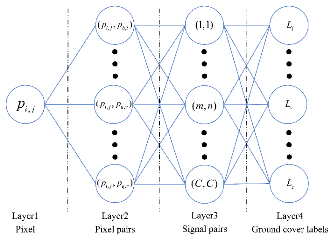
CSBN consists of four layers:
Pixel layer: composed of the target pixel and the pixels within its spatial neighborhood;
Pixel-pair layer: composed of the target pixel and a pixel within a specified neighborhood;
Signal-class-pair layer: represents the combinations in which the target pixel and its neighboring pixel belong to different signal classes;
Label layer: represents the land-cover classes obtained from the object-level image interpretation results.
Let the target pixel be denoted by pi,j, with its predefined neighborhood denoted by N(pi,j), and let a neighboring pixel be denoted by pu,v. The signal classes corresponding to the target pixel and the neighboring pixel are denoted by Wo and Wn, respectively, while the associated land-cover class is denoted by Lv.
2.5.2. Training of Conditional Probabilities for Signal-Class Pairs
For land-cover class Lv, the training set is constructed by selecting pixels with class code v from the object-level interpretation map:
where v ∈ {(1,…,v,…K}) denotes the class code, and Lv represents the v-th land-cover class.
Tv = {pi,j|Z(pi,j) = v}
Using the fuzzy memberships of the training pixels and their neighboring pixels, the fuzzy occurrence frequency of signal-class pair (ωo, ωn)within land-cover class Lv is calculated as:
where uo(pi,j) denotes the fuzzy membership degree of target pixel pi,j to signal class ωo, and un(pu,v) denotes the fuzzy membership degree of neighboring pixel pu,v to signal class ωn.
The conditional probability of signal-class pair (ωo, ωn)given land-cover class Lv is estimated as:
In this study, a uniform prior probability is assumed for all land-cover classes:
The prior probability of a signal-class pair is then calculated according to the law of total probability:
2.5.3. Pixel-Level Land-Cover Posterior Probability Estimation
Given the spectral information of the target pixel and its neighboring pixel, this study assumes that their assignments to signal classes are conditionally independent. Therefore, the probability that the target pixel pi,j and neighboring pixel pu,v belong to the signal-class pair (ωo, ωn) can be approximated as:
P((wo,wn)|(pi,j,pu,v)) = P(wo|pi,j)P(wn|pu,v)≈uo(pi,j)un(pu,v)
According to Bayes’ theorem, the posterior probability of land-cover class Lv corresponding to signal-class pair (ωo, ωn) is
Assuming that all pixel pairs within the neighborhood contribute equally to the posterior probability estimation of the target pixel, the neighborhood weight is defined as:
By integrating the neighboring pixels and all signal-class pairs, the posterior probability that target pixel pi,j belongs to land-cover class Lv is given by
Equation (31) jointly exploits the fuzzy memberships of the target pixel and its neighboring pixels to all signal classes. In this way, pixel-level spectral uncertainty can be preserved during land-cover posterior probability estimation while spatial contextual information is incorporated.
The above calculation is performed separately for the two temporal images, yielding the land-cover posterior probability vector of pixel pi,j at time t:
2.6. Change Vector Analysis in Posterior Probability Space
Post-classification comparison determines pixel changes according to whether the hard classification labels at two time points are identical. When class probabilities are close, however, hard classification may discard uncertainty information and amplify error accumulation, thereby degrading change detection accuracy. For example, suppose that the posterior probabilities of a pixel belonging to classes L1 and L2 at time t1 are 0.51 and 0.49, respectively, while those at time t2 are 0.49 and 0.51. Although the probability distributions at the two time points differ only slightly because of spectral variability within the same land-cover type, the maximum-posterior-probability criterion would assign the pixel to L1 at t1 and L2 at t2, thus incorrectly identifying it as a changed pixel.
To reduce the errors introduced by hard-label comparison, this study follows the approach of Chen et al. [15] and computes the bi-temporal change vector in the posterior probability space of land-cover classes. The posterior probability change vector of pixel pi,j is defined as:
The change magnitude is defined as the Euclidean norm of the posterior probability change vector:
After the change magnitude is calculated for all pixels, a posterior-probability change magnitude map D is obtained. Otsu’s method is then employed to automatically determine the binary segmentation threshold η, and the final change map is defined as:
Compared with hard classification methods that directly compare interpretation results, change vector analysis in posterior probability space exploits the full probability information of all land-cover classes to characterize differences in pixel states, thereby reducing misjudgments caused by slight reversals of the maximum-posterior class. Moreover, this method requires thresholding only a single change-magnitude map, without the need to set multiple independent thresholds for different change types.
2.7. Experimental Material and settings
2.7.1. Datasets
As shown in Figure 4, a total of 10 experimental data units (DS1–DS10) were used in this study. Among them, DS1–DS3 were used for ablation experiments and parameter optimization, in which the change detection performance of the proposed method was evaluated using multiple metrics, while the remaining datasets were used to assess generalization and adaptability. DS1–DS3 cover image scenes with different levels of complexity, ranging from simple to complex, which facilitates analysis of the relationship between the optimal window size of the proposed method and the spatial complexity of remote sensing imagery, as well as validation of the importance of neighborhood pixel information in the CSBN module.
The experimental datasets DS1–DS4 were obtained from the publicly available SenseEarth dataset released by SenseTime. To further evaluate the adaptability of the proposed method, several additional public datasets were introduced, including DS5 from the SECOND dataset, DS6–DS9 from the SYSU-CD dataset, and DS10 derived from Landsat-8 imagery. To ensure the accuracy of change detection, all experimental data were subjected to radiometric correction and image registration preprocessing. Detailed information for each data unit is provided below.
- (1)
- DS1–DS4: The remote sensing images at both time points are high-resolution RGB images with a size of 512 × 512 pixels and a spatial resolution of 3 m. The reference change labels are provided by the SenseEarth dataset. DS1 contains three land-cover classes: water bodies, wasteland, and buildings. DS2 contains four land-cover classes: cropland I, cropland II, buildings, and river networks. DS3 and DS4 contain three land-cover classes: vegetation, wasteland, and buildings. The four datasets represent a low-complexity natural landscape scene (DS1), medium-complexity urban–rural transition scenes (DS2 and DS3), and a high-complexity built-up land scene (DS4), thereby providing comprehensive test conditions for evaluating the performance of the proposed method under different levels of spatial complexity.
- (2)
- DS5: The spatial resolution is 5 m, and the image size is 512 × 512pixels. The reference labels are provided by the SECOND dataset. The scene contains five land-cover classes: river networks, buildings, cropland I, cropland II, and road networks, and represents a medium-complexity urban–rural transition scenario.
- (3)
- DS6–DS9: The spatial resolution is 0.5 m, and the image size is 256 × 256 pixels. The reference labels are provided by the SYSU-CD dataset. These datasets contain four land-cover classes: green areas, bare land, buildings, and lakes, and include both natural landscape and urban–rural transition scenes.
- (4)
- DS10: This dataset consists of Landsat-8 images acquired in 2016 and 2017 over Lanzhou New Area, Lanzhou City, Gansu Province, China. The spatial resolution is 30 m, and the image size is 650 × 650 pixels. Because no publicly available reference change labels are provided for this dataset, this study follows standard principles of remote sensing change detection and constructs the reference labels through visual interpretation, with reference to the labels presented in published studies that have used the same dataset.
2.7.2. Comparison Algorithms
The comparative experiments include two categories of change detection methods, namely deep learning-based methods and traditional learning-based methods, comprising a total of eleven algorithms. To evaluate the effectiveness of the proposed SEEDS-SAM-(XGB+BT)-FCM-CSBN-CVAPS framework from multiple perspectives, the proposed method is abbreviated as “SSFCC”. A brief description of each algorithm is provided in Table 1.
2.7.3. Experimental Setup
The experimental settings are summarized in Table 2. All experiments were conducted on a computer equipped with an NVIDIA GeForce RTX 4080 SUPER GPU and a 13th Gen Intel Core i7-13700KF CPU (3.40 GHz).
2.7.4. Evaluation Criteria
The performance of the change detection methods was evaluated using the following five metrics:
- (1)
- False Alarm Rate (FA): the proportion of unchanged pixels that are incorrectly classified as changed pixels.
- (2)
- Missed Detection Rate (MD): the proportion of truly changed pixels that are incorrectly classified as unchanged pixels.
- (3)
- Overall Accuracy (OA): the proportion of correctly detected changed and unchanged pixels among all pixels.
- (4)
- Kappa Coefficient (Kappa): a statistical measure that comprehensively reflects the agreement between the detection results and the reference labels.
- (5)
- F1 Score (F1): the harmonic mean of precision and recall, used to evaluate the ability of a change detection method to accurately identify and comprehensively retrieve changed regions.
Higher values of OA, Kappa, and F1 indicate better change detection performance, whereas lower values of FA and MD indicate fewer false alarms and missed detections, respectively. Therefore, these five metrics provide complementary evaluations of different change detection methods in terms of overall accuracy, agreement with the reference labels, and the balance between different types of detection errors.
3. Results
3.1. Evaluation of Low-Cost Semantic Interpretation Quality
To further evaluate the reliability of object-level semantic interpretation under limited manual annotation, approximately 10% of the superpixels in DS1, DS2, and DS3 were manually annotated, respectively, and semantic interpretation was performed within the active learning framework. The resulting interpretation maps were then compared with those obtained through complete manual semantic interpretation. The manual interpretation results were used as semantic references rather than as absolutely error-free ground-truth labels. The mean Intersection over Union (mIoU) was adopted to evaluate the consistency between the two sets of semantic interpretation results.
As shown in Figure 5, under the condition of only 10% manual annotation, the mIoU values for the two temporal images of DS1 are 50.73% and 54.27%, respectively. DS1 contains more fragmented ground objects, complex boundaries, and locally interwoven classes. The manual interpretation results therefore include a larger number of small-scale semantic units. During interpretation within the active learning framework, some small-area classes and complex boundary regions are merged or reassigned by the SAM-based spatial constraint module, reducing the mIoU to approximately 50%.
For DS2, the mIoU values are 67.25% and 56.36% for the two temporal images, respectively. The scene complexity of DS2 lies between that of DS1 and DS3, and a relatively pronounced difference is observed between the two time points. This indicates that semantic interpretation under limited labeled samples is also affected by temporal variations in spectral characteristics and changes in the spatial structure of ground objects.
For DS3, the mIoU values reach 80.40% and 78.63%, respectively. The ground-object regions in this dataset exhibit better spatial continuity, clearer object boundaries, and fewer land-cover classes, resulting in stronger within-object semantic homogeneity. Consequently, the segmentation masks generated by SAM are better aligned with the actual ground-object boundaries.
3.2. Comparative Experimental Results and Analysis
The change detection results of the different methods on DS1, DS2, and DS3 are shown in Figure 6, Figure 7, Figure 8. In the visualization, black denotes correctly identified unchanged pixels (TN), white denotes correctly identified changed pixels (TP), red denotes false-alarm pixels (FA), and green denotes missed-detection pixels (MD). The corresponding quantitative evaluation results in terms of OA, Kappa, MD, FA, and F1 are reported in Table 3.
The detection results of the different methods on DS1 are shown in Figure 6, and the corresponding quantitative evaluation results are presented in Table 3. The proposed method achieves the highest OA, Kappa, and F1 values, reaching 94.22%, 83.87%, and 87.62%, respectively. Compared with GMCD, which exhibits the second-best overall performance, the proposed method improves these three metrics by 4.04, 10.70, and 7.99 percentage points, respectively.
The different methods exhibit marked differences in FA and MD. DeepCVA achieves the lowest MD, at only 0.76%, but its FA reaches 39.51%. This indicates that the method fully exploits the ability of CVA to identify a large number of changed pixels. However, because its decision is mainly based on spectral differences between the two temporal images, pixels belonging to the same land-cover class may be incorrectly identified as changed when their spectral characteristics vary across time, resulting in a low MD but a relatively high FA.
GMCD yields FA and MD values of 17.99% and 22.61%, respectively. By integrating graph convolutional networks with metric learning to construct feature constraints, GMCD can reduce the overlap between the feature distributions of unchanged and changed pixels derived from the two temporal images. As a result, it achieves the best overall performance among the baseline methods. Nevertheless, it still cannot distinguish subtle change features in complex scenes with consistently high accuracy and stability, leaving considerable room for further improvement.
The proposed method achieves the lowest FA among all methods, at 6.44%, while its MD is 17.61%, and it also attains the highest Kappa and F1 scores. The remaining methods exhibit varying degrees of false alarms, missed detections, or a combination of both types of errors.
From the visual comparison, the proposed method preserves the major changed regions relatively completely while reducing false alarms in unchanged areas. The remaining errors are mainly concentrated along some object boundaries and in small-scale regions.
The detection results on DS2 are shown in Figure 7, and the corresponding quantitative evaluation results are presented in Table 3. The proposed method achieves OA, Kappa, and F1 values of 93.24%, 86.05%, and 91.78%, respectively, all of which are the highest among the compared methods. Compared with SGAMFNet, which exhibits the second-best overall performance, the proposed method improves these three metrics by 7.19, 9.61, and 5.56 percentage points, respectively.
DeepCVA achieves the lowest MD, at 6.26%, but its FA reaches 26.34%. SGAMFNet yields an MD of 28.66%, while GMCD achieves an FA of 11.72%. The proposed method obtains an FA of 5.09%, the lowest among all methods, together with an MD of 11.15%. The remaining methods exhibit varying increases in either FA or MD, with particularly pronounced missed detections observed for CutMix-CD, SAM-CD, and INLPG.
The visual results are generally consistent with the quantitative metrics. DeepCVA produces a relatively large number of false alarms in some unchanged regions, while several other methods exhibit obvious missed detections in changed areas. SGAMFNet generates some false alarms near the boundaries of changed regions. This is mainly because the generated pseudo-labels and the final predictions are not sufficiently accurate along object boundaries. In particular, its foreground–background separation module relies on feature differences to construct attention, while boundary features are often ambiguous, making precise localization of change contours difficult. In contrast, the proposed method preserves the major changed regions more completely while reducing false detections in the background.
Figure 8 and Table 3 present the detection results of the different methods on DS3. Compared with DS1 and DS2, most methods achieve relatively high accuracy on the DS3 scene. SSFCC attains the best overall detection performance, with OA, Kappa, and F1 values of 98.04%, 90.21%, and 91.31%, respectively. Compared with SAM-CD, which achieves the closest overall performance, SSFCC improves OA, Kappa, and F1 by 0.41, 2.79, and 2.57 percentage points, respectively. In conjunction with the results obtained on DS1 and DS2, this comparison indicates that the performance of SAM-CD is highly dependent on the suitability of its training weights for the target data, resulting in pronounced performance variation and limited generalization across different scenes and datasets.
Compared with the other baseline methods, ASEA, CCM-OBCD, INLPG, and TSSG achieve relatively low FA values, ranging from 11.67% to 18.48%, while CFRL obtains the lowest MD among the baseline methods. SSFCC achieves an MD of 6.81%, the lowest among all methods, while its FA is 10.49%, second only to that of SAM-CD. It also attains the highest Kappa and F1 scores.
From the visual results, some methods with relatively low FA still exhibit missed detections in changed regions, whereas others produce noticeable false alarms in the background. SSFCC is able to extract the major changed regions relatively completely, with the remaining errors mainly concentrated along object boundaries and in a small number of small-scale changed regions.
3.3. Sensitivity Experiments
3.3.1. Superpixel Annotation Ratio and Number of Sampled Pixels
To analyze the effects of the annotation ratio and the number of pixels sampled for CSBN training on the change detection performance of the proposed method, six annotation ratios, namely 5%, 10%, 15%, 20%, 25%, and 30%, and four sampling sizes, namely 500, 1000, 1500, and 2000 pixels, were evaluated on DS1, DS2, and DS3. To account for the influence of random sampling on the detection results, each parameter combination was independently repeated 10 times, and the mean and standard deviation of Kappa were used for evaluation.
The experimental results indicate that the annotation ratio has a relatively pronounced effect on detection performance, whereas the influence of the number of sampled pixels is comparatively limited. When the annotation ratio increases from 5% to 10%, the Kappa values on all three datasets improve markedly. This suggests that the BT strategy progressively incorporates the most informative and highly uncertain samples in the feature space into the training set, thereby rapidly refining the decision boundaries of XGBoost and correcting errors in the land-cover prior information. After these improved labels are introduced into the FCM-CSBN-CVAPS pipeline, the enhanced semantic label quality leads to a clear improvement in change detection accuracy.
When the annotation ratio is further increased from 15% to 30%, the Kappa values remain generally high and exhibit only minor fluctuations. This indicates that further increasing the annotation ratio yields limited additional performance gains. The newly added samples are likely to be largely redundant in the feature space, such that the decision boundaries of XGBoost no longer change substantially, resulting in only small variations in change detection accuracy.

Table 4.
Effects of annotation ratio and sampling size on detection accuracy (Kappa, %).
| Data | Annotation ratio | 500 | 1000 | 1500 | 2000 |
|---|---|---|---|---|---|
| DS1 | 5% | 66.73 ± 6.70 | 66.87 ± 3.67 | 65.96 ± 2.66 | 67.89 ± 3.97 |
| 10% | 83.92 ± 0.04 | 83.91 ± 0.02 | 83.90 ± 0.03 | 83.93 ± 0.03 | |
| 15% | 82.67 ± 0.08 | 82.65 ± 0.05 | 82.65 ± 0.03 | 82.66 ± 0.04 | |
| 20% | 83.80 ± 0.34 | 83.81 ± 0.32 | 83.91 ± 0.04 | 83.82 ± 0.29 | |
| 25% | 83.04 ± 0.43 | 82.91 ± 0.33 | 82.80 ± 0.05 | 82.94 ± 0.31 | |
| 30% | 83.05 ± 0.47 | 82.98 ± 0.42 | 82.96 ± 0.43 | 82.87 ± 0.29 | |
| DS2 | 5% | 66.97 ± 2.62 | 63.24 ± 1.72 | 64.88 ± 1.26 | 64.49 ± 1.88 |
| 10% | 85.84 ± 0.15 | 85.79 ± 0.15 | 85.90 ± 0.15 | 85.77 ± 0.14 | |
| 15% | 85.55 ± 0.12 | 85.49 ± 0.07 | 85.48 ± 0.05 | 85.47 ± 0.02 | |
| 20% | 83.59 ± 2.19 | 84.92 ± 1.15 | 85.10 ± 0.56 | 85.29 ± 0.05 | |
| 25% | 84.34 ± 3.11 | 85.14 ± 0.82 | 85.36 ± 0.24 | 85.46 ± 0.05 | |
| 30% | 85.07 ± 1.17 | 85.52 ± 0.12 | 85.50 ± 0.06 | 85.48 ± 0.04 | |
| DS3 | 5% | 85.66 ± 0.90 | 86.33 ± 0.98 | 85.99 ± 0.73 | 86.25 ± 0.04 |
| 10% | 89.35 ± 0.71 | 88.83 ± 0.61 | 89.28 ± 0.86 | 88.79 ± 0.67 | |
| 15% | 88.55 ± 0.65 | 88.25 ± 0.08 | 88.42 ± 0.52 | 88.37 ± 0.52 | |
| 20% | 88.45 ± 0.79 | 88.69 ± 0.05 | 88.69 ± 0.06 | 88.73 ± 0.09 | |
| 25% | 87.95 ± 1.10 | 88.58 ± 0.07 | 88.34 ± 0.77 | 88.36 ± 0.77 | |
| 30% | 88.52 ± 0.74 | 88.78 ± 0.07 | 88.80 ± 0.06 | 88.54 ± 0.78 |
Note: The results are reported as mean ± SD, with each parameter configuration independently repeated 10 times. Bold values indicate the highest mean Kappa coefficient for the corresponding dataset.
3.4.2. Fuzziness Coefficient and Number of Signal Classes
To analyze the effects of the FCM fuzziness coefficient (q) and the number of signal classes on the change detection performance of the proposed method, a controlled variable strategy was adopted. The fuzziness coefficient and the number of signal classes were varied while all other parameters were kept unchanged, and the Kappa coefficient was used to evaluate the detection performance under different parameter combinations. The experimental results are shown in Figure 9.
The experimental results show that when q < 2, the Kappa values of both SSFCC and SSFSC are generally low across all three datasets. As q increases, the Kappa values generally exhibit an initial increase, followed by a slight decline and then a gradual stabilization. This trend indicates that when q is too small, the model has difficulty characterizing the fuzzy transition information associated with mixed pixels and class boundaries. When q increases to an appropriate range, mixed pixels can be more reasonably decomposed and inter-class fuzziness can be effectively represented. Beyond the optimal range, however, the membership degrees become overly uniform, which weakens inter-class differences and leads to a slight decrease in accuracy before the performance stabilizes. Overall, when q lies in the range of 2.5–3.0, the detection performance on all three datasets remains at a relatively high level.
Under different settings for the number of signal classes, the Kappa values of both methods exhibit some fluctuations, but the overall magnitude of variation remains relatively limited. Compared with SSFSC, SSFCC achieves higher Kappa values under most parameter combinations and maintains strong overall detection performance across different settings of q and the number of signal classes. These results indicate that, within the parameter ranges examined in this study, the fuzziness coefficient has a more pronounced influence on detection performance, whereas the number of signal classes has a comparatively smaller effect.
3.4.3. Window Size
This section investigates the effect of window size on change detection performance, with the fuzziness coefficient fixed at q = 3. The results are shown in Figure 10. Overall, a larger window does not necessarily lead to better performance. Although a larger neighborhood can incorporate richer spatial contextual information, once the window extends beyond a locally homogeneous region, it may also include pixels belonging to different land-cover classes, thereby weakening local contextual consistency and introducing a certain degree of spatial over-smoothing.
Specifically, for scenes with relatively simple spatial structures and fewer land-cover classes, such as DS3, a relatively small window is sufficient to achieve a high Kappa coefficient. In contrast, for scenes with more complex spatial structures and more fragmented land-cover distributions, appropriately increasing the window size helps exploit more comprehensive neighborhood information and thus improves change detection performance. The experimental results indicate that the optimal window size varies across different scenes, and more complex scenes generally require larger neighborhoods to capture sufficient contextual information. As the window size continues to increase, some heterogeneous pixels may be incorporated into the contextual region, resulting in a slight decline in detection performance. Thereafter, the variation in the Kappa coefficient gradually decreases and the overall performance tends to stabilize.
3.4. Adaptive Evaluation
To further evaluate the detection performance of the proposed method across different remote sensing scenarios, experiments were conducted on seven datasets, DS4–DS10, and the results were compared with those of 11 change detection methods. The visual results are shown in Figure 11, and the corresponding quantitative evaluation results are presented in Table 5. Overall, the baseline methods exhibit substantial performance variations across the different datasets, whereas SSFCC achieves the highest Kappa and F1 scores on all seven datasets from DS4 to DS10.
On DS4, the scene contains four land-cover classes—roads, bare land, buildings, and vegetation—and is also affected by shadows cast by ground objects, which poses additional challenges for change detection. CCM-OBCD is the best-performing baseline, mainly owing to its effective suppression of false alarms. However, this method employs a random forest classifier and is therefore a supervised machine learning approach that depends heavily on training samples. Moreover, the method was primarily evaluated for forest-to-bare-land changes, and its performance decreases for other types of change, such as changes involving buildings and water bodies. As shown in Figure 11, CCM-OBCD exhibits relatively severe missed detections in building-change regions.
For DS5 and DS7, GMCD is the best-performing baseline. As shown in Figure 11, on DS5, both GMCD and SSFCC miss some small changed regions; however, SSFCC suppresses scattered false alarms more effectively. Consequently, the Kappa and F1 scores of SSFCC are 3.08 and 2.24 percentage points higher than those of GMCD, respectively. On DS7, SSFCC exhibits fewer missed-detection areas, extracts the changed regions more completely, and substantially reduces false-alarm regions, resulting in improvements of 12.08 and 8.83 percentage points in Kappa and F1, respectively.
For DS6, DS9, and DS10, Table 5 shows that SGAMFNet is the best-performing baseline. Across these three datasets, the mean Kappa and F1 scores of SSFCC are 7.45 and 6.46 percentage points higher than those of SGAMFNet, respectively. As illustrated in Figure 11, DeepCVA produces the most severe false alarms on DS6, whereas the other methods exhibit varying degrees of missed detections. Both SSFCC and SGAMFNet miss some pixels along the boundaries of changed regions; however, SSFCC is more effective at suppressing scattered false alarms and therefore achieves better overall performance. On DS9, SGAMFNet produces larger missed-detection regions than SSFCC, resulting in lower detection accuracy. On DS10, both SSFCC and SGAMFNet exhibit varying degrees of missed detections and false alarms, but SSFCC achieves a better balance between missed-detection control and false-alarm suppression.
For DS8, KPCAMNet is the best-performing baseline; however, its Kappa and F1 scores are relatively low, at 65.77% and 70.31%, respectively, which are 25.19 and 21.73 percentage points lower than those of SSFCC. This indicates that the nonlinear kernel function has difficulty adapting to the land-cover distribution and radiometric characteristics of this scene, thereby limiting the method’s ability to discriminate differences in pixel-level semantic information and resulting in relatively poor detection performance.
Across the seven datasets, SSFCC achieves the highest overall detection accuracy, with mean Kappa and F1 scores of 84.73% and 87.88%, respectively. These results indicate that its advantages are not confined to a single scene, but are consistently maintained across different land-cover compositions, spatial structures, and change scales, demonstrating strong adaptability to diverse remote sensing scenarios.
3.5. Ablation Experiments
To further investigate the contributions of different modules in the proposed framework to change detection performance, nine ablation or replacement variants, denoted as Algorithms 2–10, were constructed based on Algorithm 1 and evaluated on the DS1, DS2, and DS3 datasets. The main configurations and validation objectives of these variants are summarized in Table 6 and Table 7. Algorithms 2–6 are primarily designed to analyze the effects of spatial constraints, image interpretation strategies, and annotation schemes on detection performance, whereas Algorithms 7–10 are used to evaluate the contributions of different probabilistic modeling and feature representation mechanisms in the change detection stage.
Algorithm 3 uses 100% manual annotation and is therefore mainly included as a reference for analyzing the relationship between annotation cost and detection performance, rather than being interpreted as a strict single-variable ablation.
The quantitative evaluation results of the different algorithms on DS1, DS2, and DS3 are presented in Table 8, and the corresponding visual results are shown in Figure 12. Overall, Algorithm 1 achieves the highest OA, Kappa, and F1 on all three datasets, with mean Kappa and F1 values of 86.71% and 90.24%, respectively, outperforming all other variants. These results indicate that the individual modules within the complete framework do not merely provide additive improvements; rather, they interact synergistically to determine the final change detection performance.
3.5.1. Effect of the Spatial Constraint Module
The comparison between Algorithms 1 and 2 shows that removing the SAM-based spatial constraint leads to a decline in detection performance on all three datasets, with the largest decrease observed on DS2. This indicates that the labels of most superpixels are predicted correctly, while only a small number of small-area superpixels are misclassified. Within each segmentation mask, the dominant class usually occupies an overwhelming proportion of the area and can therefore override a small number of isolated misclassified superpixels. In this way, the spatial constraint suppresses scattered classification noise without disrupting the underlying structure of real ground objects.
Algorithms 4 and 5 provide another comparison for evaluating the effect of spatial constraints. On DS2, Algorithm 5 achieves a clear improvement after introducing the spatial constraint, and a certain performance gain is also observed on DS3. However, on DS1, Algorithm 4 performs slightly better than Algorithm 5. This suggests that the spatial constraint module can correct small misclassified samples, but may also suppress small correctly classified samples. Its effectiveness therefore depends largely on whether ambiguous samples near object boundaries can be handled appropriately. When such boundary samples are incorporated into a segmentation mask with imperfect semantic assignment, a small number of correctly classified superpixels within the mask may also be overridden.
For DS1, Algorithm 2 performs slightly worse than Algorithm 1 in the absence of spatial constraints. Under the 10% annotation setting, active learning selects a relatively large number of ambiguous superpixels during training, which helps refine the classification boundary for boundary samples. However, a small number of misclassified superpixels may still occur within locally homogeneous regions. Without the SAM-based spatial constraint for correction, these misclassified patches can perturb the local posterior probability vectors during CSBN-based spatial estimation, thereby leading to erroneous change decisions. The behavior of SVM is somewhat different: most samples within homogeneous regions are classified correctly, whereas ambiguous samples are less accurately predicted, although a small number of correctly classified samples are preserved. As a result, its performance is slightly higher than that of Algorithm 2 but still lower than that of Algorithm 1.
As shown in Figure 12, models without spatial constraints produce more scattered false alarms or missed detections along some object boundaries and background regions, whereas the changed regions obtained after introducing the spatial constraint are generally more spatially continuous.
3.5.2. Effects of Image Interpretation and Annotation Strategies
The results of Algorithms 1, 5, and 6 show that different image interpretation strategies can substantially affect the subsequent change detection performance. Under the 10% annotation setting, Algorithm 1 achieves higher overall performance than Algorithms 5 and 6 on all three datasets, with the differences being more pronounced on DS2 and DS3. This is mainly attributable to differences in sample selection strategies.
Algorithm 6 adopts K-means, which selects samples based only on distances in the spectral feature space and therefore tends to cover representative samples near the centers of major classes. However, boundary and ambiguous samples, which often contribute most to improving classification accuracy, are not preferentially selected. Algorithm 5 employs SVM with random sampling. This strategy places relatively high demands on the annotator’s experience and domain knowledge, because the sampled set may contain mostly easily recognizable samples while including only a limited number of ambiguous samples. Consequently, the SVM decision boundary lacks sufficient constraints from samples in confusion regions, resulting in weaker generalization performance.
Algorithm 3 uses 100% manual annotation as a reference for examining the relationship between annotation cost and detection performance. In contrast, Algorithm 1 achieves comparable or even higher overall detection performance with a much lower annotation ratio. Because Algorithms 1 and 3 differ simultaneously in spatial constraints and semantic acquisition strategies, this comparison is used only as a reference for annotation cost and is not interpreted as a strict single-variable ablation.
3.5.3. Effects of the Change Detection Module
Algorithms 7–10 are used to evaluate the roles of different modeling mechanisms in the change detection stage. Algorithm 7 yields lower Kappa and F1 scores than Algorithm 1 on all three datasets and exhibits varying degrees of false alarms or missed detections. Although Algorithm 7 has demonstrated strong performance on medium-spatial-resolution imagery [13], high-resolution imagery contains richer spatial information. By incorporating spatial contextual information into change detection, Algorithm 1 substantially reduces the false alarm rate.
Algorithm 8 still achieves relatively high detection performance on DS1 but shows a marked decline on DS2 and DS3. Although SVM improves classification accuracy through optimization of the decision boundary, it tends to produce posterior probability vectors with relatively low uncertainty. As a result, some land-cover classes may receive excessively high posterior probabilities, which can lead to overestimation of changed pixels and consequently increase the false alarm rate. In contrast, Algorithm 1 consistently achieves the best overall performance across all three datasets.
Algorithm 9 provides better control of missed detections than Algorithm 1 on all three datasets. However, after CSBN outputs posterior probability vectors, Algorithm 9 applies the maximum a posteriori (MAP) criterion, which discards fuzzy information and determines sample labels solely according to the largest posterior probability, after which PCC is used to determine whether a change has occurred. Algorithm 10 directly adopts PCC and is therefore similarly affected by the accumulation of classification errors. Consequently, both Algorithms 9 and 10 exhibit degraded performance and increased false alarm rates, which is consistent with the findings reported by Li [13,44].
3.5.4. Overall Analysis
Overall, Algorithm 1 achieves the highest OA, Kappa, and F1 scores on DS1–DS3, with mean Kappa and F1 values of 86.71% and 90.24%, respectively. Although some ablation variants show local advantages in either FA or MD, their overall evaluation metrics remain lower than those of Algorithm 1. These results provide experimental evidence for the contributions of the different components to the performance of the complete framework. Since Algorithms 1 and 3 differ simultaneously in terms of spatial constraints and semantic acquisition strategies, their comparison is used only as a reference for annotation cost and is not interpreted as a strict single-variable ablation.
4. Discussion
The proposed method integrates object-level spatial organization, few-shot semantic interpretation, and the FCM-CSBN-CVAPS framework to reduce annotation costs and improve change detection accuracy for high-spatial-resolution remote sensing imagery. Reliable object-level semantic priors are constructed from a limited amount of manual semantic annotation, while contextual posterior probability inference is used to suppress the direct propagation of local interpretation errors. In this way, the method achieves a favorable balance between controlling missed detections and suppressing false alarms, thereby improving the stability of change detection in complex remote sensing scenes.
During the image interpretation stage, although the consistency between the proposed method and complete manual interpretation varies considerably across different scenes, the major spatial semantic structures of ground objects can still be effectively recovered. These results are sufficient to provide valid semantic priors for the posterior probability model at a relatively low manual cost and to supply land-cover prior information for CSBN. SEEDS-guided SAM segmentation organizes the image into spatially contiguous objects and provides regional consistency constraints for superpixel classification results. Using superpixels as the basic processing units, XGBoost is employed as the classifier, while samples with high classification uncertainty are preferentially selected for manual annotation, enabling superpixel classification within an active learning framework.
The annotation-ratio sensitivity experiments show that, when the annotation ratio reaches approximately 10%, the detection performance enters a relatively high and stable range, while the gains obtained by further increasing the annotation ratio gradually diminish. When the number of labeled samples is insufficient, the training set cannot adequately cover the spectral characteristics of all land-cover classes. As representative and highly uncertain samples are progressively incorporated into the training set, the classifier is able to obtain more stable semantic information. Because FCM-CSBN-CVAPS performs change measurement using fuzzy memberships, spatial context, and land-cover posterior probabilities, it can, to some extent, reduce the direct influence of local semantic interpretation errors on change detection accuracy compared with methods that directly compare hard classification labels. These results indicate that, under the experimental conditions of this study, complete manual semantic interpretation is not required to provide effective semantic information for posterior probability-based change detection, thereby demonstrating the practical value of object-level active interpretation in reducing semantic annotation costs. Moreover, although the proposed method does not achieve the lowest FA and MD simultaneously in every scene, the use of pixel-level fuzzy information and spatial contextual inference enables a favorable balance between missed-detection control and false-alarm suppression. This is one of the reasons why the method maintains stable overall performance across scenes with different spatial resolutions, land-cover compositions, and change scales.
The parameter sensitivity experiments further show that the FCM fuzziness coefficient and the CSBN neighborhood size should be maintained within appropriate ranges. In particular, an excessively large neighborhood may introduce heterogeneous land-cover information and weaken local spatial consistency, indicating that parameter settings remain influenced by the spatial structural characteristics of the imagery.
Nevertheless, the proposed method still has several limitations. First, the performance gain provided by object-level spatial constraints is scene-dependent. The comparison between Algorithms 4 and 5 in the ablation experiments shows that, for scenes with more fragmented spatial structures, more complex object boundaries, or stronger spectral heterogeneity, object-level spatial constraints provide more evident improvements in change detection accuracy; otherwise, the gain is relatively limited. Second, the current CSBN mainly exploits local neighborhood information and remains limited in representing long-range spatial dependencies. Third, parameters such as the SEEDS segmentation scale, FCM parameters, and neighborhood window size still require adjustment according to image characteristics, and segmentation errors or missed detections may still occur in regions with complex boundaries or small-scale changes. Future work may further improve the method through lightweight object segmentation, parallel probabilistic computation, adaptive parameter selection, and modeling of larger-scale spatial relationships, thereby enhancing its level of automation and applicability across diverse remote sensing scenarios.
5. Conclusions
To address the challenges of spectral uncertainty, insufficient exploitation of spatial information, and the dependence of probability-based change detection on manually acquired semantic training information in high-resolution remote sensing imagery, this study proposes a change detection framework that integrates vision foundation model-assisted interpretation with contextual Bayesian inference. The proposed method uses SEEDS superpixels to guide SAM in constructing object partitions, employs XGBoost together with a breaking-ties active query strategy to obtain object-level semantic information under limited manual supervision, and further integrates the fuzzy spectral representation of FCM, the spatial contextual inference of CSBN, and change analysis in the posterior probability space to achieve the final change detection result.
Considering that FCM-CSBN-CVAPS, when applied to high-resolution remote sensing imagery, relies on manually acquired semantic information to exploit pixel-level fuzzy information and spatial information for posterior probability-based land-cover change measurement, this study develops a change detection framework that integrates SEEDS-guided SAM object construction, active learning-based interpretation, and FCM-CSBN-CVAPS posterior probability inference. The proposed method obtains object-level land-cover semantic information with only a small amount of manual annotation and subsequently combines fuzzy spectral information representation, spatial contextual inference, and change measurement in the posterior probability space to perform bi-temporal change detection.
The experimental results show that the proposed method achieves Kappa values of 83.87%–90.21% and F1 scores of 87.62%–91.78% on DS1–DS3. Across the seven multi-scenario datasets DS4–DS10, the mean Kappa and F1 reach 84.73% and 87.88%, respectively. The annotation-ratio sensitivity experiments indicate that semantic annotation of approximately 10% of the superpixels is sufficient for the detection performance to enter a relatively high and stable range. The ablation experiments further verify the contributions of object-level spatial constraints, active semantic interpretation, and contextual probabilistic modeling to the performance of the complete framework. Overall, the experimental results demonstrate that combining low-cost object-level semantic acquisition with pixel-level posterior probability-based change analysis can reduce the demand for complete manual semantic interpretation while maintaining stable change detection performance, thereby providing a feasible solution for high-spatial-resolution remote sensing image change detection under limited annotation conditions.
References
- Cheng, G.; Wang, G.X.; Han, J.W. Deep learning for change detection in remote sensing: A review and new outlooks. Natl. Remote Sens. Bull. 2025, 29, 1587–1597. [Google Scholar] [CrossRef]
- Zhang, J.X.; Gu, H.Y.; Yang, Y.; Zhang, H.; Li, H.T. Research progress and trend of high-resolution remote sensing imagery intelligent interpretation. Natl. Remote Sens. Bull. 2021, 25, 2198–2210. [Google Scholar] [CrossRef]
- Chen, P.; Li, C.; Zhang, B.; Chen, Z.; Yang, X.; Lu, K.; Zhuang, L. A region-based feature fusion network for VHR image change detection. Remote Sens. 2022, 14, 5577. [Google Scholar] [CrossRef]
- Wang, J.; Zhao, T.; Jiang, X.; Lan, K. A hierarchical heterogeneous graph for unsupervised SAR image change detection. IEEE Geosci. Remote Sens. Lett. 2022, 19, 4516605. [Google Scholar] [CrossRef]
- Zhao, H.; Liu, S.; Du, Q.; Bruzzone, L.; Zheng, Y.; Du, K.; Tong, X.; Xie, H.; Ma, X. GCFnet: Global collaborative fusion network for multispectral and panchromatic image classification. IEEE Trans. Geosci. Remote Sens. 2022, 60, 5632814. [Google Scholar] [CrossRef]
- Zhang, H.; Yao, J.; Ni, L.; Gao, L.; Huang, M. Multimodal attention-aware convolutional neural networks for classification of hyperspectral and LiDAR data. IEEE J. Sel. Top. Appl. Earth Obs. Remote Sens. 2023, 16, 3635–3644. [Google Scholar] [CrossRef]
- Ma, J.; Gong, M.; Zhou, Z. Wavelet fusion on ratio images for change detection in SAR images. IEEE Geosci. Remote Sens. Lett. 2012, 9, 1122–1126. [Google Scholar] [CrossRef]
- Deng, J.S.; Wang, K.; Deng, Y.H.; Qi, G.J. PCA-based land-use change detection and analysis using multitemporal and multisensor satellite data. Int. J. Remote Sens. 2008, 29, 4823–4838. [Google Scholar] [CrossRef]
- Bovolo, F.; Bruzzone, L. A theoretical framework for unsupervised change detection based on change vector analysis in the polar domain. IEEE Trans. Geosci. Remote Sens. 2007, 45, 218–236. [Google Scholar] [CrossRef]
- Ronneberger, O.; Fischer, P.; Brox, T. U-Net: Convolutional networks for biomedical image segmentation. In Medical Image Computing and Computer-Assisted Intervention—MICCAI 2015; Lecture Notes in Computer Science; Navab, N., Hornegger, J., Wells, W.M., Frangi, A.F., Eds.; Springer: Cham, Switzerland, 2015; Volume 9351, pp. 234–241. [Google Scholar] [CrossRef]
- Zhao, Q.; Zhang, J.; Zheng, W. A combined method of PCA and IR-MAD for detecting rainfall landslide. Bull. Surv. Mapp. 2024, 5, 7–11. [Google Scholar] [CrossRef]
- Hao, M.; Zhang, H.; Shi, W.; Deng, K. Unsupervised change detection using fuzzy c-means and MRF from remotely sensed images. Remote Sens. Lett. 2013, 4, 1185–1194. [Google Scholar] [CrossRef]
- Li, Y.K.; Yang, Y.; Yang, S.W.; Wang, Z.H. A change vector analysis in posterior probability space combined with fuzzy C-means clustering and a Bayesian network. Remote Sens. Nat. Resour. 2021, 33, 82–88. [Google Scholar] [CrossRef]
- Hussain, M.; Chen, D.; Cheng, A.; Wei, H.; Stanley, D. Change detection from remotely sensed images: From pixel-based to object-based approaches. ISPRS J. Photogramm. Remote Sens. 2013, 80, 91–106. [Google Scholar] [CrossRef]
- Chen, J.; Chen, X.; Cui, X.; Chen, J. Change vector analysis in posterior probability space: A new method for land cover change detection. IEEE Geosci. Remote Sens. Lett. 2011, 8, 317–321. [Google Scholar] [CrossRef]
- Tang, X.; Zhang, H.; Mou, L.; Liu, F.; Zhang, X.; Zhu, X.X.; Jiao, L. An unsupervised remote sensing change detection method based on multiscale graph convolutional network and metric learning. IEEE Trans. Geosci. Remote Sens. 2022, 60, 5609715. [Google Scholar] [CrossRef]
- Wu, C.; Chen, H.; Du, B.; Zhang, L. Unsupervised change detection in multitemporal VHR images based on deep kernel PCA convolutional mapping network. IEEE Trans. Cybern. 2022, 52, 12084–12098. [Google Scholar] [CrossRef]
- Saha, S.; Bovolo, F.; Bruzzone, L. Unsupervised deep change vector analysis for multiple-change detection in VHR images. IEEE Trans. Geosci. Remote Sens. 2019, 57, 3677–3693. [Google Scholar] [CrossRef]
- Liu, T.; Zhang, M.; Gong, M.; Zhang, Q.; Jiang, F.; Zheng, H.; Lu, D. Commonality feature representation learning for unsupervised multimodal change detection. IEEE Trans. Image Process. 2025, 34, 1219–1233. [Google Scholar] [CrossRef]
- Shu, Q.; Zhu, X.; Wan, L.; Zhao, S.; Liu, D.; Peng, L.; Chen, X. CutMix-CD: Advancing semi-supervised change detection via mixed sample consistency. IEEE Trans. Geosci. Remote Sens. 2025, 63, 4400915. [Google Scholar] [CrossRef]
- Ding, L.; Zhu, K.; Peng, D.; Tang, H.; Yang, K.; Bruzzone, L. Adapting Segment Anything Model for change detection in VHR remote sensing images. IEEE Trans. Geosci. Remote Sens. 2024, 62, 5611711. [Google Scholar] [CrossRef]
- Han, Y.; Li, J.; Qu, Y.; et al. HFNet: Semantic and Differential Heterogenous Fusion Network for Remote Sensing Image Change Detection. J. Geovisualization Spat. Anal. 2025, 9(1), 1. [Google Scholar] [CrossRef]
- Zhou, P.C.; Cheng, G.; Yao, X.W.; Han, J.W. Machine learning paradigms in high-resolution remote sensing image interpretation. Natl. Remote Sens. Bull. 2021, 25, 182–197. [Google Scholar] [CrossRef]
- Liu, S.C.; Du, K.C.; Zheng, Y.J.; Chen, J.; Du, P.J.; Tong, X.H. Remote sensing change detection technology in the era of artificial intelligence: Inheritance, development and challenges. Natl. Remote Sens. Bull. 2023, 27, 1975–1987. [Google Scholar] [CrossRef]
- Wang, L.; Zhang, M.; Shi, W. STCRNet: A semi-supervised network based on self-training and consistency regularization for change detection in VHR remote sensing images. IEEE J. Sel. Top. Appl. Earth Obs. Remote Sens. 2024, 17, 2272–2282. [Google Scholar] [CrossRef]
- Chen, G.; He, C.; Wang, T.; Zhu, K.; Liao, P.; Zhang, X. A superpixel-guided unsupervised fast semantic segmentation method of remote sensing images. IEEE Geosci. Remote Sens. Lett. 2022, 19, 2506605. [Google Scholar] [CrossRef]
- Zhou, M. Research on the superpixel-based change detection methods based on remote sensing images. Master’s Thesis, China University of Mining and Technology, Xuzhou, China, May 2021. [Google Scholar]
- Wang, Y.H.; Gao, L.R.; Chen, Z.C.; Zhang, B. Deep learning and superpixel-based method for high-resolution remote sensing image change detection. J. Image Graph. 2020, 25, 1271–1282. [Google Scholar] [CrossRef]
- Liu, S.Y.; Zhao, Y.L. DP-SAM: Efficient semantic segmentation of remote sensing images by fine-tuning SAM. J. Image Graph. 2025, 30, 2884–2896. [Google Scholar] [CrossRef]
- Kirillov, A.; Mintun, E.; Ravi, N.; Mao, H.; Rolland, C.; Gustafson, L.; Xiao, T.; Whitehead, S.; Berg, A.C.; Lo, W.-Y.; Dollár, P.; Girshick, R. Segment Anything. In Proceedings of the IEEE/CVF International Conference on Computer Vision (ICCV), Paris, France, 1–6 October 2023; pp. 4015–4026. [Google Scholar] [CrossRef]
- Gui, B.; Bhardwaj, A.; Sam, L. Evaluating the efficacy of Segment Anything Model for delineating agriculture and urban green spaces in multiresolution aerial and spaceborne remote sensing images. Remote Sens. 2024, 16, 414. [Google Scholar] [CrossRef]
- Tian, J.; Cai, W.; Sun, Z.; Wang, Y. Unsupervised change detection in remote sensing images using an integrated SAM and MAD method. J. Indian Soc. Remote Sens. 2026, 54, 3605–3622. [Google Scholar] [CrossRef]
- Jiang, W.; Sun, Y.; Lei, L.; Kuang, G.; Ji, K. AdaptVFMs-RSCD: Advancing remote sensing change detection from binary to semantic with SAM and CLIP. ISPRS J. Photogramm. Remote Sens. 2025, 230, 304–317. [Google Scholar] [CrossRef]
- Zhang, X.; Li, D.; Xia, Y.; Dong, X.; Yu, H.; Wang, J.; Li, Q. OmniOVCD: Streamlining open-vocabulary change detection with SAM 3. arXiv 2026, arXiv:2601.13895. [Google Scholar] [CrossRef]
- Fang, L.; Kuang, Y.; Liu, Q.; Yue, J. Temporal difference prompted SAM for remote sensing change detection. J. Signal Process. 2024, 40, 417–427. [Google Scholar] [CrossRef]
- Tang, J.; Tong, H.; Tong, F.; Zhang, Y.; Chen, W. Exploiting superpixel-based contextual information on active learning for high spatial resolution remote sensing image classification. Remote Sens. 2023, 15, 715. [Google Scholar] [CrossRef]
- Shao, P.; Fan, H.M.; Gao, Z.A. An adaptive and semi-supervised fuzzy C-means clustering algorithm for remotely sensed change detection. J. Geo-Inf. Sci. 2022, 24, 508–521. [Google Scholar] [CrossRef]
- Deng, W.; Chen, X.; Hai, T.; Wu, T.; Ye, C.; Wang, H. Semi-supervised remote sensing image change detection based on feature refinement and consistency. J. Guangxi Univ. Nat. Sci. Ed. 2025, 50, 1058–1072. [Google Scholar] [CrossRef]
- Settles, B. Active Learning Literature Survey; Computer Sciences Technical Report 1648; University of Wisconsin–Madison: Madison, WI, USA, 2009. [Google Scholar]
- Yoo, D.; Kweon, I.S. Learning loss for active learning. In Proceedings of the IEEE/CVF Conference on Computer Vision and Pattern Recognition (CVPR), Long Beach, CA, USA, 16–20 June 2019; pp. 93–102. [Google Scholar] [CrossRef]
- Van den Bergh, M.; Boix, X.; Roig, G.; Van Gool, L. SEEDS: Superpixels extracted via energy-driven sampling. Int. J. Comput. Vis. 2015, 111, 298–314. [Google Scholar] [CrossRef]
- Lv, X.; Ming, D.; Chen, Y.Y.; Wang, M. Very high resolution remote sensing image classification with SEEDS-CNN and scale effect analysis for superpixel CNN classification. Int. J. Remote Sens. 2019, 40, 506–531. [Google Scholar] [CrossRef]
- Li, Y.; Bretschneider, T.R. Semantic-sensitive satellite image retrieval. IEEE Trans. Geosci. Remote Sens. 2007, 45, 853–860. [Google Scholar] [CrossRef]
- Li, Y.; Li, X.; Song, J.; Wang, Z.; He, Y.; Yang, S. Remote-sensing-based change detection using change vector analysis in posterior probability space: A context-sensitive Bayesian network approach. IEEE J. Sel. Top. Appl. Earth Obs. Remote Sens. 2023, 16, 3198–3217. [Google Scholar] [CrossRef]
- Zhu, R.; Li, Y.K.; Li, X.J.; Yang, S.W.; Xie, J.L. Multivariate alteration detection using angle thresholds based on a context-sensitive Bayesian network. Remote Sens. Nat. Resour. 2025, 37, 131–140. [Google Scholar] [CrossRef]
- Lv, Z.; Wang, F.; Liu, T.; Kong, X.; Benediktsson, J.A. Novel automatic approach for land cover change detection by using VHR remote sensing images. IEEE Geosci. Remote Sens. Lett. 2022, 19, 8016805. [Google Scholar] [CrossRef]
- Zhu, Z.; Zhou, T.; Chen, J.; Li, X.; Guo, S.; Zhao, L.; Sun, L. Object-oriented remote sensing image change detection based on color co-occurrence matrix. Appl. Sci. 2023, 13, 6748. [Google Scholar] [CrossRef]
- Sun, Y.; Lei, L.; Li, X.; Tan, X.; Kuang, G. Structure consistency-based graph for unsupervised change detection with homogeneous and heterogeneous remote sensing images. IEEE Trans. Geosci. Remote Sens. 2022, 60, 4700221. [Google Scholar] [CrossRef]
- Wu, J.; Ni, W.; Bian, H.; Cheng, K.; Liu, Q.; Kong, X.; Li, B. Unsupervised change detection for VHR remote sensing images based on temporal-spatial-structural graphs. Remote Sens. 2023, 15, 1770. [Google Scholar] [CrossRef]
- Liu, Y.; You, Z.-H.; Chen, S.-B.; Wang, X.; Xu, L.-X.; Tang, J.; Luo, B. SAM-guided attention maps fusion for region supervised remote sensing image change detection. IEEE J. Sel. Top. Appl. Earth Obs. Remote Sens. 2025, 18, 24518–24530. [Google Scholar] [CrossRef]
Figure 1.
Overall workflow of the object-level active interpretation and posterior probability-based change detection method.
Figure 1.
Overall workflow of the object-level active interpretation and posterior probability-based change detection method.
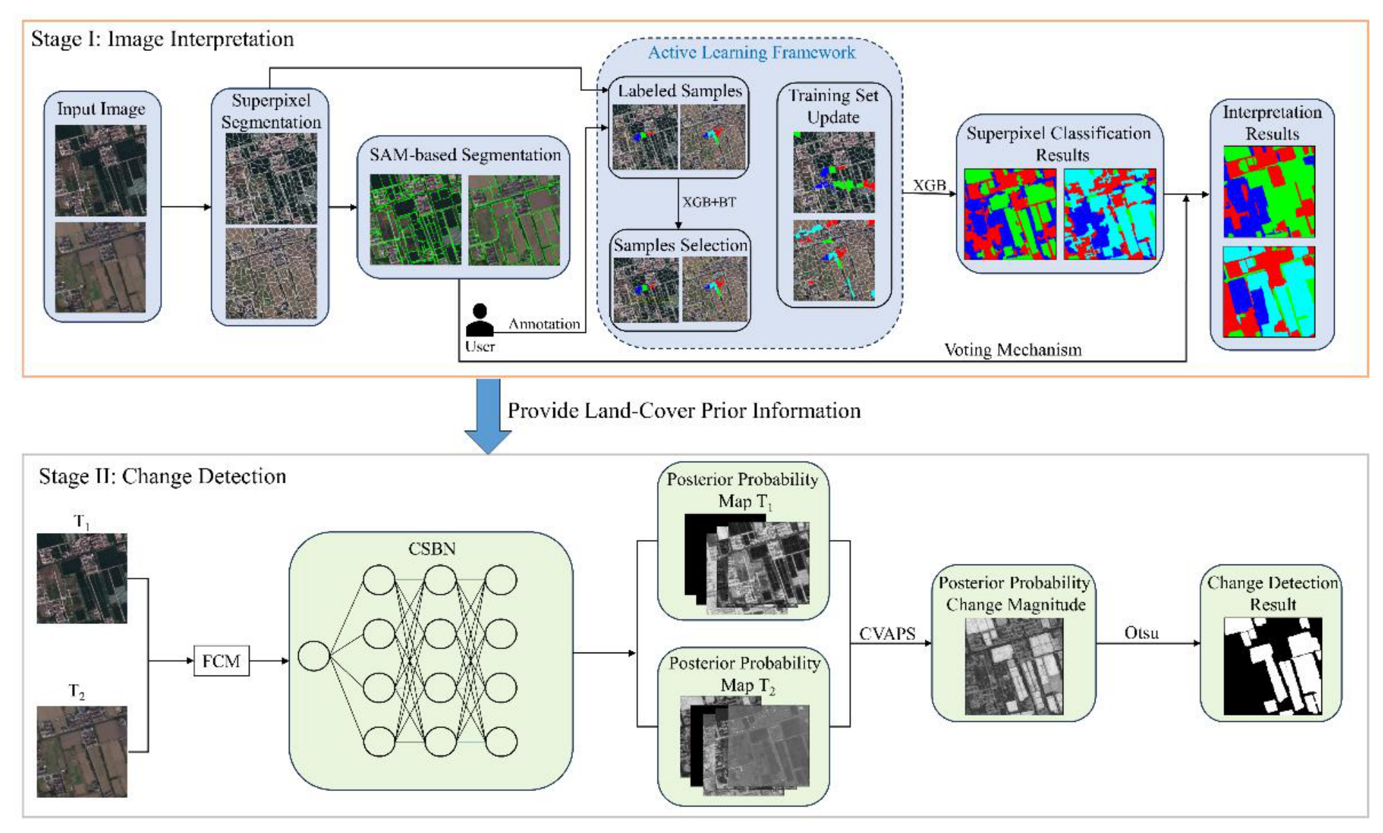
Figure 4.
. Experimental datasets.
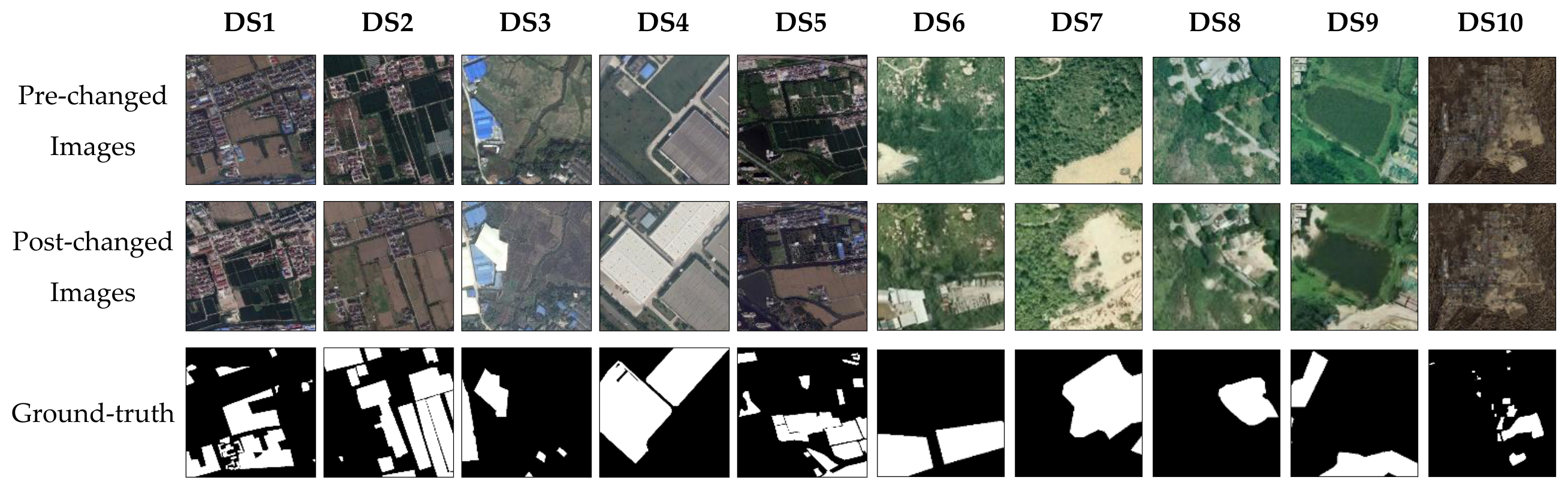
Figure 5.
Comparison of SSFCC and manual interpretation results.
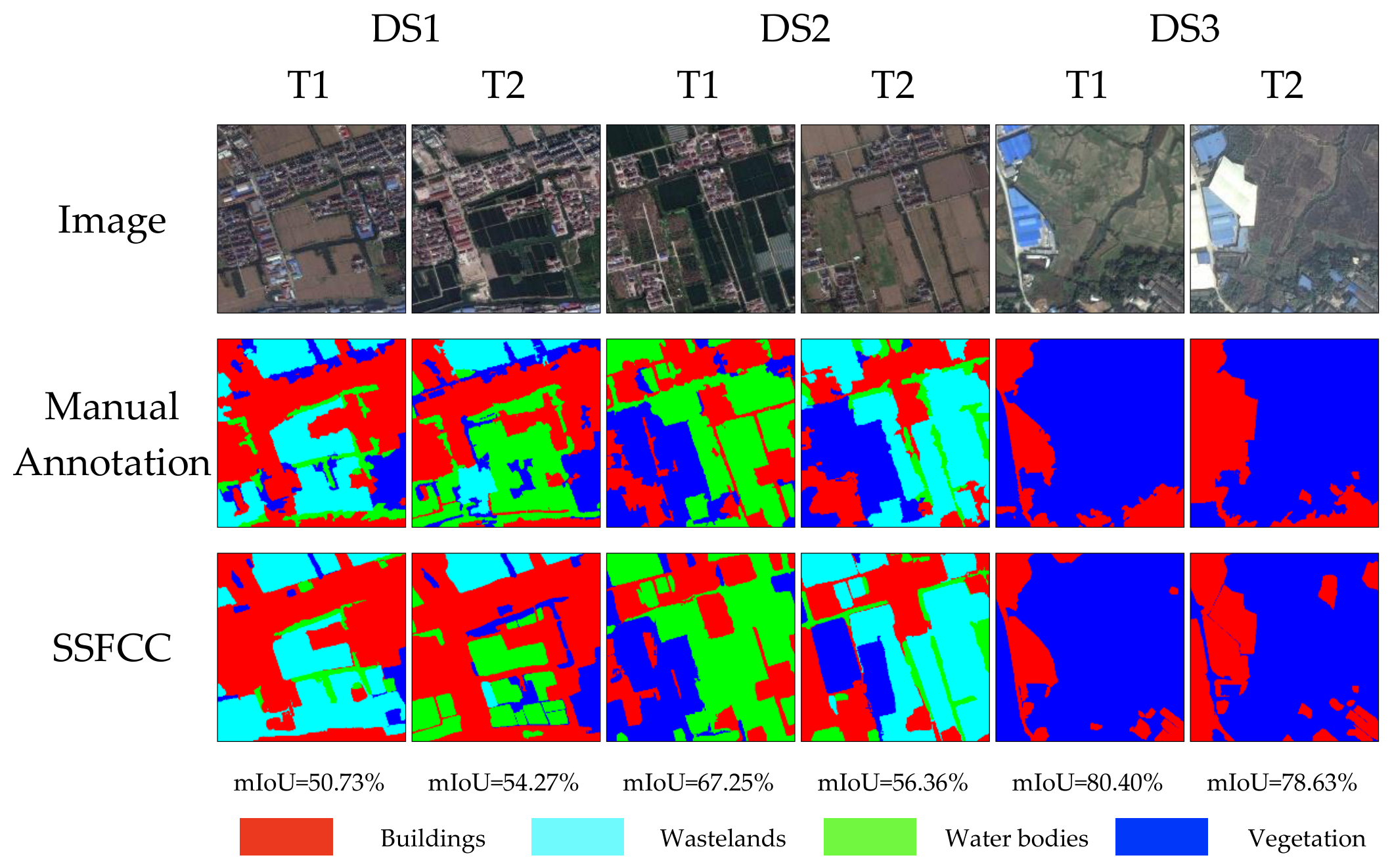
Figure 6.
Change detection results on DS1. (a) DeepCVA; (b) GMCD; (c) KPCAMNet; (d) CFRL; (e) CutMix-CD; (f) SAM-CD; (g) ASEA; (h) CCM-OBCD; (i) INLPG; (j) TSSG; (k) SGAMFNet; (l) SSFCC.
Figure 6.
Change detection results on DS1. (a) DeepCVA; (b) GMCD; (c) KPCAMNet; (d) CFRL; (e) CutMix-CD; (f) SAM-CD; (g) ASEA; (h) CCM-OBCD; (i) INLPG; (j) TSSG; (k) SGAMFNet; (l) SSFCC.
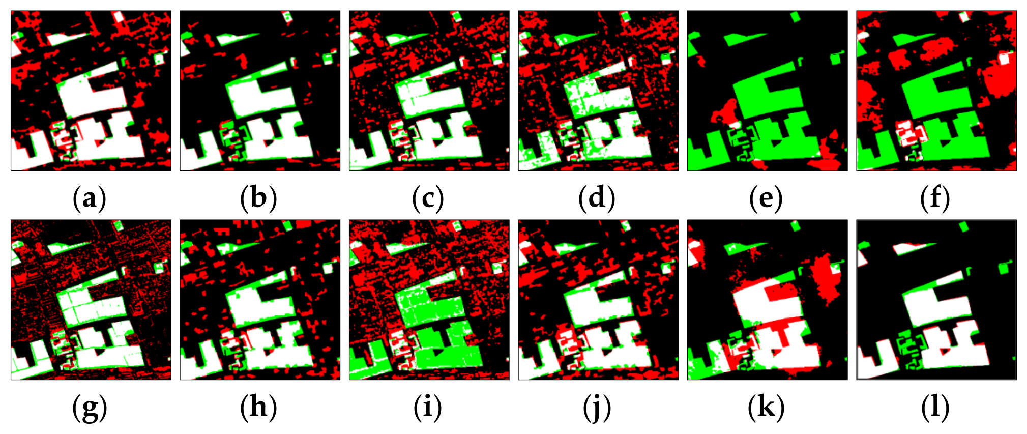
Figure 7.
Change detection results on DS2. (a) DeepCVA; (b) GMCD; (c) KPCAMNet; (d) CFRL; (e) CutMix-CD; (f) SAM-CD; (g) ASEA; (h) CCM-OBCD; (i) INLPG; (j) TSSG; (k) SGAMFNet; (l) SSFCC.
Figure 7.
Change detection results on DS2. (a) DeepCVA; (b) GMCD; (c) KPCAMNet; (d) CFRL; (e) CutMix-CD; (f) SAM-CD; (g) ASEA; (h) CCM-OBCD; (i) INLPG; (j) TSSG; (k) SGAMFNet; (l) SSFCC.
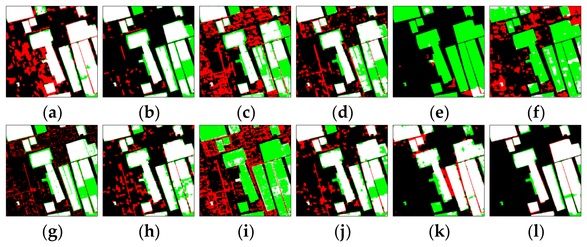
Figure 8.
Change detection results on DS3. (a) DeepCVA; (b) GMCD; (c) KPCAMNet; (d) CFRL; (e) CutMix-CD; (f) SAM-CD; (g) ASEA; (h) CCM-OBCD; (i) INLPG; (j) TSSG; (k) SGAMFNet; (l) SSFCC.
Figure 8.
Change detection results on DS3. (a) DeepCVA; (b) GMCD; (c) KPCAMNet; (d) CFRL; (e) CutMix-CD; (f) SAM-CD; (g) ASEA; (h) CCM-OBCD; (i) INLPG; (j) TSSG; (k) SGAMFNet; (l) SSFCC.
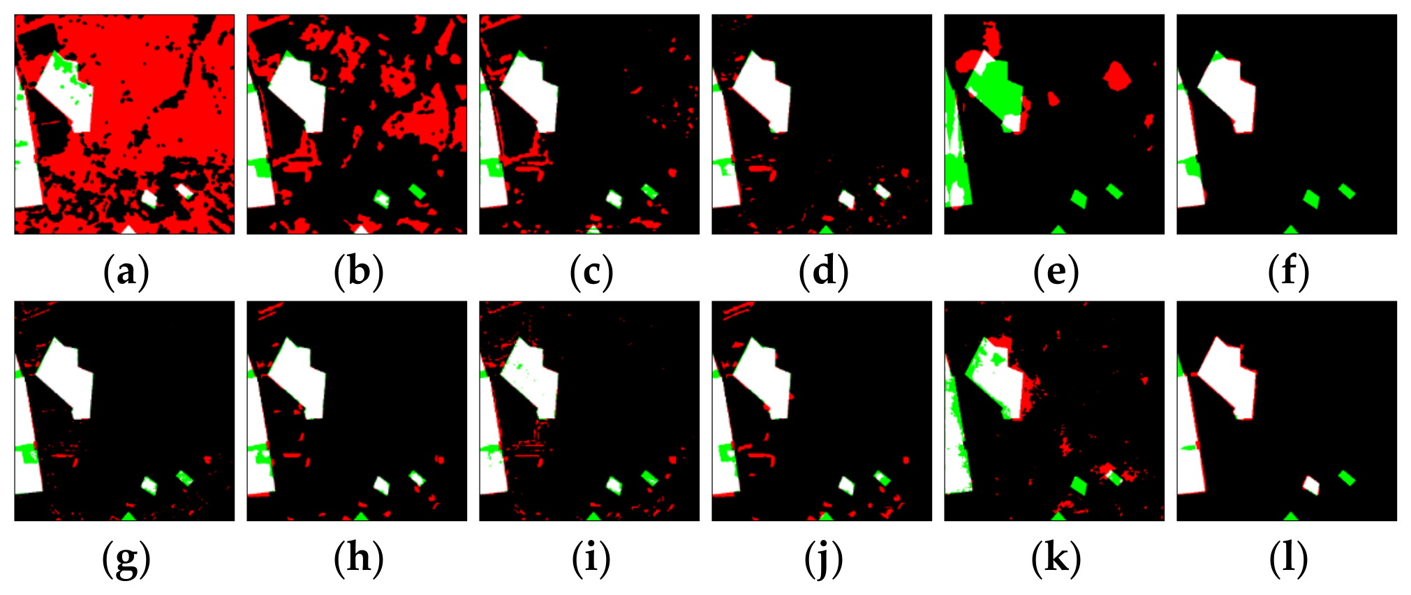
Figure 9.
Effect of the fuzziness weighting coefficient q on the change detection performance of the proposed method.
Figure 9.
Effect of the fuzziness weighting coefficient q on the change detection performance of the proposed method.
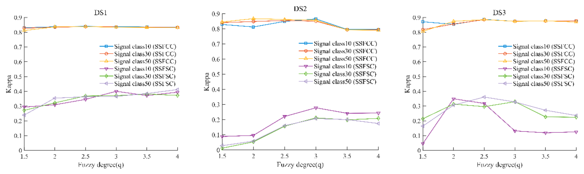
Figure 10.
Effect of window size on the change detection performance of the proposed method.
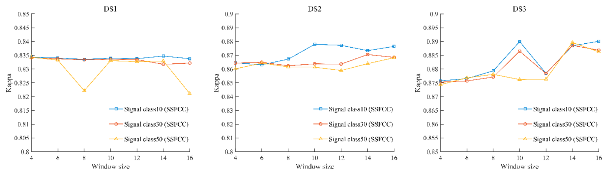
Figure 11.
Change detection accuracy of the compared methods on DS4–DS10.
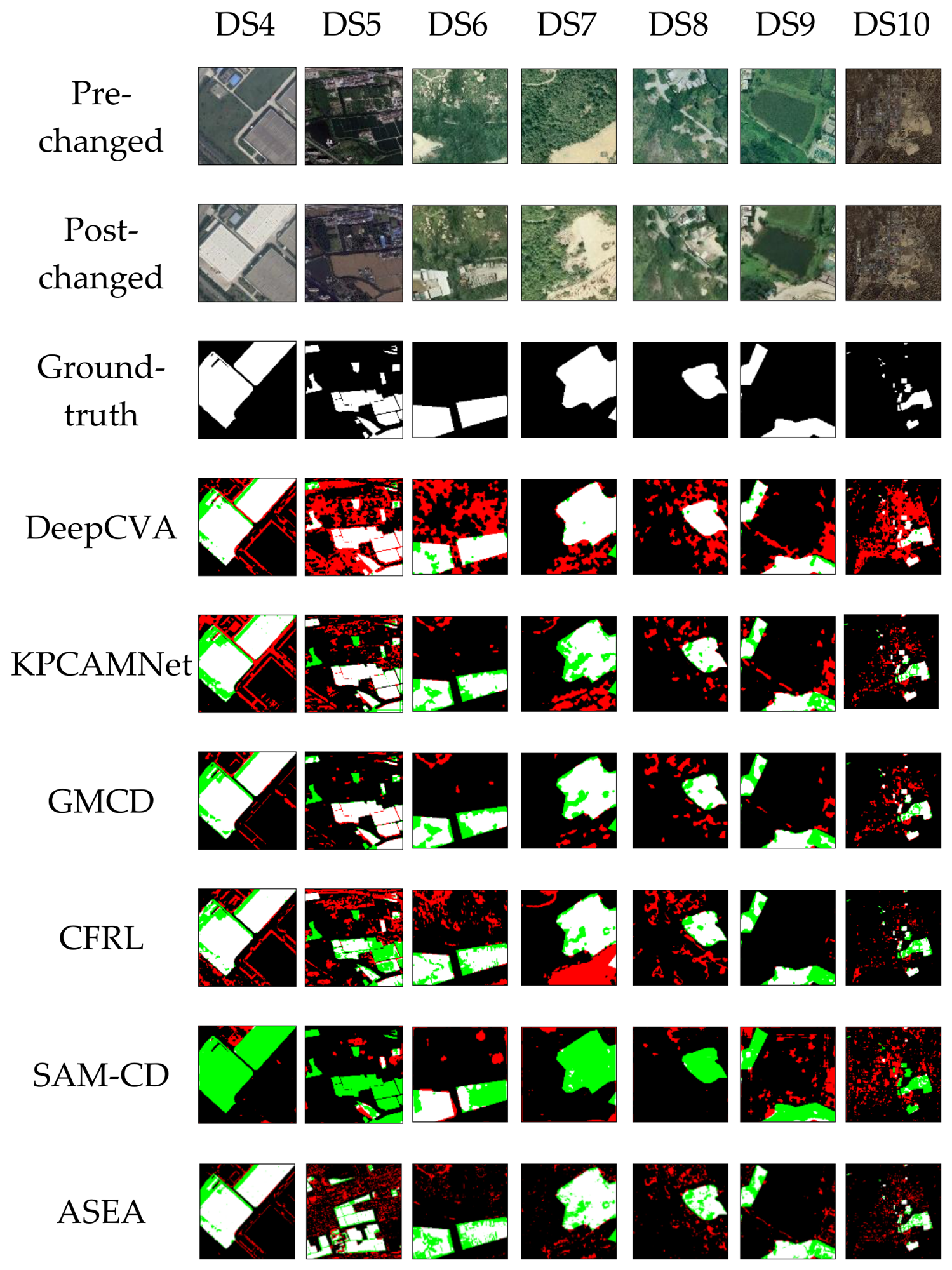
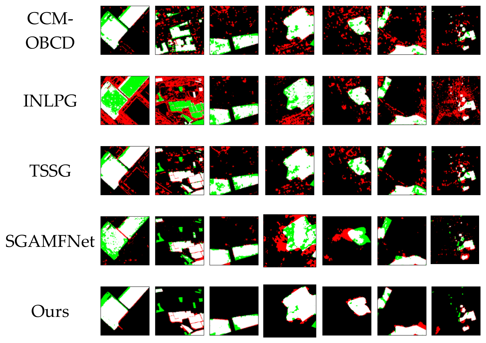
Figure 12.
Results of the ablation experiments.
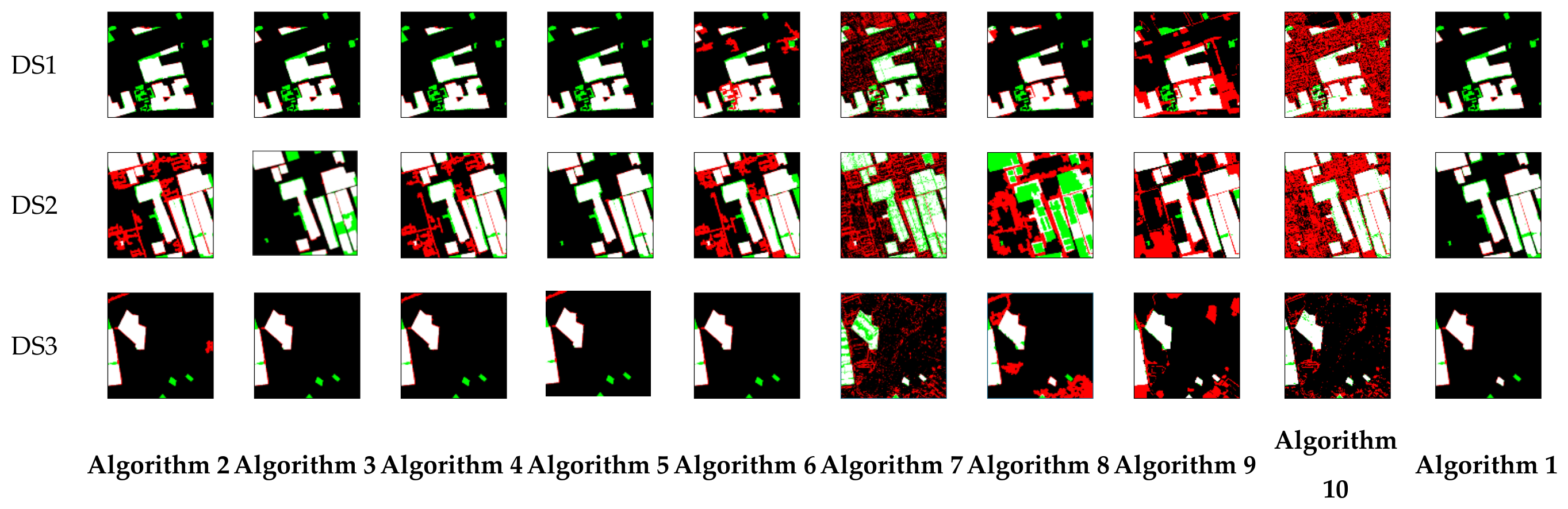
Table 1.
Brief descriptions of the compared algorithms.
| Algorithm | Description |
|---|---|
| DeepCVA [18] | An unsupervised context-aware change detection framework constructed using features extracted from a pretrained convolutional neural network. |
| KPCAMNet [17] | A method integrating kernel principal component analysis with a deep Siamese mapping network, capable of both binary and multiclass change detection. |
| GMCD [16] | An unsupervised change detection method combining graph convolutional networks with metric learning. |
| SAM-CD [21] | A fully supervised remote sensing change detection method that adopts FastSAM as the backbone to transfer the general semantic priors of SAM, employs convolutional adapters for remote sensing domain adaptation, and introduces a task-agnostic temporal learning branch. |
| CutMix-CD [20] | A semi-supervised remote sensing change detection method that extracts multiscale change features using a ResNet-CD Siamese network, augments change samples through change-aware CutMix, and employs an exponential moving average (EMA) teacher for consistency regularization. |
| CFRL [19] | An unsupervised multimodal remote sensing change detection method that performs cross-modal alignment using a Siamese encoder–decoder architecture, jointly learns domain-invariant features through multilevel reconstruction losses, and detects changes based on metric features. |
| ASEA [46] | A high-resolution remote sensing change detection method that adaptively constructs spatial contextual regions for each pixel and derives change magnitude by comparing the multispectral mean differences between corresponding regions in bi-temporal images. |
| CCM-OBCD [47] | An object-based change detection method that uses a color co-occurrence matrix to extract spectral and textural features of image objects and employs a classifier to determine whether the corresponding bi-temporal objects have changed. |
| INLPG [48] | A change detection method that constructs nonlocal neighborhood graphs from bi-temporal images and compares the consistency of corresponding graph structures, identifying rgions with significant structural changes as changed areas. |
| TSSG [49] | A method that constructs a spatiotemporal structural graph by integrating temporal, spatial, and multiscale structural relationships between bi-temporal images, and detects land-cover changes based on differences in graph nodes and neighborhood structures. |
| SGAMFNet [50] | A weakly supervised remote sensing change detection method that generates regional pseudo-labels from bi-temporal image difference information using the Segment Anything Model (SAM) and integrates multiscale change features through an attention mechanism, without requiring pixel-level annotations. |
Table 2.
Experimental settings.
| Method | Learning Paradigm | Weight Source | Training Data |
|---|---|---|---|
| DeepCVA | Unsupervised | Open-source code | – |
| GMCD | Unsupervised | Open-source code | – |
| KPCAMNet | Unsupervised | Open-source code | – |
| CFRL | Unsupervised | Open-source code | – |
| CutMix-CD | Semi-supervised | Trained from scratch | LEVIR-CD, WHU-CD, and the datasets compiled in this study |
| SAM-CD | Fully supervised | Released by the authors | LEVIR-CD and WHU-CD |
| ASEA | Unsupervised | None | – |
| CCM-OBCD | Fully supervised | Open-source code | – |
| INLPG | Unsupervised | None | – |
| TSSG | Unsupervised | None | – |
| SGAMFNet | Weakly supervised | Official SAM ViT-H pretrained weights; ImageNet-pretrained ResNet18 | Bi-temporal images of the target scene and region-level weak supervision labels generated by SAM |
| Ours | Active learning-assisted | None | A small number of manually annotated superpixel samples |
Table 3.
Accuracy of change detection results on DS1, DS2, and DS3.
| Data | Algorithm | OA | Kappa | MD | FA | F1 |
|---|---|---|---|---|---|---|
| DS1 | DeepCVA | 83.14% | 61.59% | 0.76% | 39.51% | 73.11% |
| GMCD | 90.18% | 73.17% | 22.61% | 17.99% | 79.63% | |
| KPCAMNet | 79.77% | 51.79% | 22.20% | 43.26% | 65.62% | |
| CFRL | 75.81% | 41.40% | 32.86% | 49.05% | 57.93% | |
| CutMix-CD | 71.24% | - | 98.77% | 93.31% | 2.08% | |
| SAM-CD | 60.16% | - | 89.94% | 87.55% | 11.11% | |
| ASEA | 79.57% | 51.29% | 22.63% | 43.56% | 65.27% | |
| CCM-OBCD | 82.93% | 56.21% | 26.35% | 35.99% | 67.71% | |
| INLPG | 56.23% | - | 75.69% | 80.55% | 21.61% | |
| TSSG | 80.76% | 54.92% | 17.33% | 42.13% | 68.08% | |
| SGAMFNet | 81.16% | 53.13% | 26.44% | 40.21% | 65.96% | |
| Ours | 94.22% | 83.87% | 17.61% | 6.44% | 87.62% | |
| DS2 | DeepCVA | 83.10% | 66.60% | 6.26% | 26.34% | 82.50% |
| GMCD | 85.32% | 69.05% | 28.66% | 7.61% | 80.51% | |
| KPCAMNet | 63.78% | 27.20% | 35.74% | 43.50% | 60.13% | |
| CFRL | 77.34% | 53.11% | 30.98% | 24.45% | 72.14% | |
| CutMix-CD | 57.90% | 1.88% | 96.36% | 42.52% | 6.84% | |
| SAM-CD | 48.44% | - | 87.13% | 72.65% | 17.50% | |
| ASEA | 82.04% | 62.79% | 25.94% | 18.06% | 77.80% | |
| CCM-OBCD | 84.69% | 68.71% | 17.25% | 18.12% | 82.07% | |
| INLPG | 43.17% | - | 85.13% | 76.57% | 18.19% | |
| TSSG | 82.59% | 64.17% | 22.69% | 19.13% | 79.05% | |
| SGAMFNet | 88.56% | 76.44% | 15.75% | 11.72% | 86.22% | |
| Ours | 93.24% | 86.05% | 11.15% | 5.09% | 91.78% | |
| DS3 | DeepCVA | 36.85% | 5.77% | 10.64% | 86.26% | 23.81% |
| GMCD | 78.82% | 37.24% | 13.93% | 67.39% | 47.30% | |
| KPCAMNet | 93.75% | 72.02% | 12.69% | 33.46% | 75.52% | |
| CFRL | 96.90% | 85.10% | 7.33% | 18.28% | 86.85% | |
| CutMix-CD | 87.74% | 24.46% | 75.38% | 59.12% | 30.74% | |
| SAM-CD | 97.63% | 87.42% | 15.45% | 6.64% | 88.74% | |
| ASEA | 97.37% | 86.56% | 12.24% | 11.67% | 88.04% | |
| CCM-OBCD | 96.98% | 83.73% | 12.40% | 15.02% | 85.41% | |
| INLPG | 96.48% | 82.86% | 10.74% | 19.15% | 84.85% | |
| TSSG | 96.57% | 83.21% | 10.89% | 18.48% | 85.15% | |
| SGAMFNet | 93.67% | 67.94% | 28.07% | 28.92% | 71.50% | |
| Ours | 98.04% | 90.21% | 6.81% | 10.49% | 91.31% |
Note: The best result for each indicator is shown in bold, and the second-best result is underlined.
Table 5.
Adaptability evaluation results of the compared methods on DS4–DS10.
| DeepCVA | GMCD | KPCAMNet | CFRL | CutMix-CD | SAM-CD | |||||||
| Kappa | F1 | Kappa | F1 | Kappa | F1 | Kappa | F1 | Kappa | F1 | Kappa | F1 | |
| DS4 | 69.24% | 82.74% | 74.20% | 84.50% | 48.78% | 71.44% | 21.41% | 80.88% | 22.48% | 45.81% | - | 1.33% |
| DS5 | 33.45% | 56.10% | 76.04% | 81.83% | 58.97% | 70.33% | 23.66% | 43.79% | - | 28.31% | 0.82% | 9.71% |
| DS6 | 36.42% | 58.08% | 66.89% | 74.10% | 70.89% | 77.53% | 57.18% | 68.95% | 9.81% | 15.71% | 54.32% | 64.57% |
| DS7 | 74.77% | 83.35% | 77.68% | 84.03% | 57.96% | 68.66% | 48.70% | 67.20% | 3.91% | 28.76% | - | 6.26% |
| DS8 | 47.43% | 55.83% | 60.13% | 65.46% | 65.77% | 70.31% | 48.79% | 56.18% | 5.54% | 10.61% | - | 1.17% |
| DS9 | 61.83% | 70.10% | 63.70% | 69.39% | 55.46% | 63.76% | 64.58% | 69.18% | - | 1.62% | - | 14.42% |
| DS10 | 25.96% | 33.90% | 52.86% | 56.74% | 54.72% | 58.46% | 53.05% | 56.21% | 7.24% | 9.88% | 0.09% | 9.16% |
| ASEA | CCM-OBCD | INLPG | TSSG | SGAMFNet | SSFCC | |||||||
| Kappa | F1 | Kappa | F1 | Kappa | F1 | Kappa | F1 | Kappa | F1 | Kappa | F1 | |
| DS4 | 77.71% | 86.70% | 80.15% | 87.87% | - | 34.86% | 75.78% | 86.13% | 68.00% | 79.55% | 86.17% | 91.68% |
| DS5 | 65.38% | 74.57% | 69.23% | 76.27% | - | 14.78% | 63.02% | 73.18% | 72.27% | 78.45% | 79.12% | 84.07% |
| DS6 | 60.99% | 69.49% | 66.84% | 74.98% | 73.21% | 79.48% | 69.00% | 76.23% | 84.81% | 88.59% | 89.46% | 92.04% |
| DS7 | 74.80% | 82.11% | 68.79% | 79.20% | 55.70% | 69.98% | 76.67% | 83.85% | 40.20% | 59.63% | 89.76% | 92.86% |
| DS8 | 55.22% | 60.86% | 48.34% | 55.45% | 63.57% | 68.50% | 56.67% | 62.34% | 41.43% | 48.40% | 90.96% | 92.04% |
| DS9 | 62.36% | 68.37% | 54.32% | 64.21% | 63.51% | 71.00% | 66.91% | 72.89% | 77.10% | 80.94% | 84.45% | 87.37% |
| DS10 | 52.07% | 55.79% | 54.91% | 57.94% | 28.38% | 35.94% | 57.84% | 61.27% | 62.81% | 65.57% | 73.16% | 75.08% |
Table 6.
Description of the algorithms included in the ablation experiments.
| No. | Algorithm | Description |
|---|---|---|
| 1 | SSFCC | The proposed change detection algorithm |
| 2 | SEEDS-(XGBoost+BT)-FCC | The spatial constraint module SAM is removed. |
| 3 | SEEDS-ManualAnnotation-FCC | The spatial constraint module SAM is removed, and the “XGBoost+BT” classification strategy is replaced with manual annotation, abbreviated as “MA”. |
| 4 | SEEDS-SVM-FCC | The spatial constraint module SAM is removed, and the “XGBoost+BT” classification strategy is replaced with SVM. |
| 5 | SEEDS-SAM-SVM-FCC | The spatial constraint module SAM is retained, while the “XGBoost+BT” classification strategy is replaced with SVM. |
| 6 | SEEDS-SAM-Kmeans-FCC | The “XGBoost+BT” classification strategy is replaced with K-means. |
| 7 | SEEDS-SAM-(XGBoost+BT)-FSC | In the FCC change detection module, CSBN is replaced with SBN, and “FCM-SBN-CVAPS” is abbreviated as “FSC”. |
| 8 | SEEDS-SAM-(XGBoost+BT)-SC | In the FCC change detection module, FCM and CSBN are replaced with SVM, and “SVM-CVAPS” is abbreviated as “SC”. |
| 9 | SEEDS-SAM-(XGBoost+BT)-PCC | The entire FCM-CSBN-CVAPS change detection module is replaced with PCC. |
| 10 | SEEDS-SAM-(XBGoost+BT)-FCP | The FCM-CSBN-CVAPS change detection module is replaced with FCM-CSBN-PCC, abbreviated as “FCP”. |
Table 7.
Ablation experiment settings and objectives.
| Algorithm | Modification Relative to Algorithm 1 | Comparison | Objective |
|---|---|---|---|
| Algorithm 1 | Complete framework | —— | Full model |
| Algorithm 2 | Remove the spatial constraint module | 1 vs 2 | Evaluate the contribution of spatial constraints |
| Algorithm 3 | Use 100% manual annotation as a reference | 2 vs 3;1 vs 3 | Analyze annotation cost versus performance |
| Algorithm 4 | Remove spatial constraints and replace the classifier | 2 vs 4 | Analyze the classification strategy |
| Algorithm 5 | Retain spatial constraints and replace the classifier | 4 vs 5; 1vs 5 | Evaluate spatial constraints and classification strategy |
| Algorithm 6 | Replace active interpretation with unsupervised clustering | 1 vs 6 | Evaluate the role of supervised semantic acquisition |
| Algorithm 7 | Replace the spatial probabilistic modeling component | 1 vs 7 | Evaluate spatial-context probabilistic inference |
| Algorithm 8 | Replace the back-end change detection structure | 1 vs 8 | Evaluate the overall back-end modeling strategy |
| Algorithm 9 | Replace the back-end change detection structure | 1 vs 9;8 vs 9 | Evaluate the overall back-end modeling strategy |
| Algorithm 10 | Replace CVAPS with PCC | 1 vs10 | Evaluate the contribution of CVAPS |
Table 8.
Accuracy of the algorithms in the ablation experiments.
| Data | Algorithm | Parameter | Annotation ratio | OA | Kappa | MD | FA | F1 |
|---|---|---|---|---|---|---|---|---|
| DS1 | 1 | 10 Signal class, Samples=1000, q=2.5, window size=3 |
10 | 94.22% | 83.87% | 17.61% | 6.44% | 87.62% |
| 2 | 10 Signal class, Samples=1000, q=2.5, window size=3 |
10 | 93.86% | 82.62% | 20.38% | 5.17% | 86.56% | |
| 3 | 10 Signal class, Samples=1000, q=2.5, window size=3 |
100 | 93.82% | 82.45% | 20.77% | 4.98% | 86.41% | |
| 4 | 10 Signal class, CP=15, gamma=0.5, Samples=1000, q=2.5, window size=3 | 10 | 94.20% | 83.74% | 18.30% | 5.84% | 87.49% | |
| 5 | 10 Signal class, CP=15, gamma=0.5, Samples=1000, q=2.5, window size=3 | 10 | 93.81% | 82.41% | 20.96% | 4.80% | 86.37% | |
| 6 | 10 Signal class, n=5, Samples=1000,q=2.5, window size=3 | 10 | 89.36% | 73.41% | 10.65% | 26.50% | 80.65% | |
| 7 | 50 Signal class, Sample=1000, q=4, window size=10 |
10 | 73.40% | 41.17% | 21.98% | 52.21% | 59.27% | |
| 8 | CP=15, gamma=0.5, Samples=2000 | 10 | 91.86% | 78.60% | 13.52% | 18.24% | 84.06% | |
| 9 | 10 Signal class, Samples=1000, q=2.5, window size=3 |
10 | 77.42% | 49.73% | 15.08% | 47.20% | 65.12% | |
| 10 | 10 Signal class, Samples=1000, q=2.5, window size=3 |
10 | 52.40% | 18.76% | 10.81% | 66.99% | 48.19% | |
| DS2 | 1 | 10 Signal class, Sample=1000, q=3, window size=3 |
10 | 93.24% | 86.05% | 11.15% | 5.09% | 91.78% |
| 2 | 10 Signal class, Samples=1000, q=3, window size=3 |
10 | 78.00% | 56.88% | 9.12% | 31.93% | 77.84% | |
| 3 | 10 Signal class, Samples=1000, q=3, window size=3 |
100 | 91.06% | 81.38% | 17.21% | 4.43% | 88.72% | |
| 4 | 10 Signal class, CP=15, gamma=0.5,Samples=1000, q=3, window size=3 | 10 | 78.96% | 58.34% | 11.86% | 29.94% | 78.07% | |
| 5 | 10 Signal class, CP=15, gamma=0.5,Samples=1000, q=3, window size=3 | 10 | 92.36% | 84.22% | 12.40% | 5.99% | 90.69% | |
| 6 | 10 Signal class, n=5, Samples=1000, q=3, window size=3 | 10 | 76.21% | 53.28% | 11.94% | 33.34% | 75.88% | |
| 7 | 10 Signal class, Sample=1000, q=3, window size=10 |
10 | 63.27% | 27.85% | 27.24% | 44.86% | 62.74% | |
| 8 | CP=13, gamma=20, Sample=2000 | 10 | 53.50% | 4.29% | 57.02% | 54.93% | 44.00% | |
| 9 | 10 Signal class, Sample=1000, q=3, window size=3 |
10 | 76.23% | 54.14% | 4.75% | 34.95% | 77.30% | |
| 10 | 10 Signal class, Sample=1000, q=3, window size=3 |
10 | 58.08% | 22.68% | 7.42% | 49.63% | 65.24% | |
| DS3 | 1 | 10 Signal class, Sample=1000, q=2.5, window size=3 |
10 | 98.04% | 90.21% | 6.81% | 10.49% | 91.31% |
| 2 | 10 Signal class, Samples=1000, q=2.5, window size=3 |
10 | 96.58% | 83.30% | 10.64% | 18.54% | 85.23% | |
| 3 | 10 Signal class, Samples=1000, q=2.5, window size=3 |
100 | 97.73% | 88.44% | 10.41% | 10.16% | 89.71% | |
| 4 | 10 Signal class, CP=15, gamma=0.5, samples=1000, q=2.5, window size=3 | 10 | 97.17% | 85.87% | 10.50% | 14.48% | 87.47% | |
| 5 | 10 Signal class, CP=15, gamma=0.5, samples=1000, q=2.5, window size=3 | 10 | 97.20% | 86.03% | 10.35% | 14.35% | 87.60% | |
| 6 | 10 Signal class, n=5, Samples=1000,q=2.5, window size=3 | 10 | 97.71% | 88.35% | 10.35% | 10.37% | 89.64% | |
| 7 | 50 Signal class, Sample=1000, q=2.5,window size=10 | 10 | 82.20% | 36.11% | 32.88% | 65.65% | 45.44% | |
| 8 | CP=15, gamma=0.5, Sample=2000 | 10 | 89.19% | 59.58% | 7.65% | 49.43% | 65.35% | |
| 9 | 10 Signal class, Sample=1000, q=2.5, window size=3 |
10 | 88.83% | 59.29% | 5.25% | 50.31% | 65.19% | |
| 10 | 10 Signal class, Sample=1000, q=2.5, window size=3 |
10 | 90.84% | 63.92% | 8.11% | 44.88% | 68.90% |
Disclaimer/Publisher’s Note: The statements, opinions and data contained in all publications are solely those of the individual author(s) and contributor(s) and not of MDPI and/or the editor(s). MDPI and/or the editor(s) disclaim responsibility for any injury to people or property resulting from any ideas, methods, instructions or products referred to in the content. |
© 2026 by the authors. Licensee MDPI, Basel, Switzerland. This article is an open access article distributed under the terms and conditions of the Creative Commons Attribution (CC BY) license (http://creativecommons.org/licenses/by/4.0/).
Copyright: This open access article is published under a Creative Commons CC BY 4.0 license, which permit the free download, distribution, and reuse, provided that the author and preprint are cited in any reuse.