

Submitted:
10 October 2026
Posted:
12 October 2026
You are already at the latest version
Abstract
The quantum measurement problem asks how the smooth, unitary evolution of a superposition gives way to a single, definite outcome when a macroscopic detector interacts with a quantum system. This paper presents a geometric toy model of this interaction, with a deterministic factorization stage and a probabilistic selection step. The entangled state of a quantum system and a detector is embedded into semi-structured complex (ℍ) state space, where newly introduced projection operators, called trigger transformations, factorize the entangled state into a tensor product of two identical subsystems: one describing the quantum system and one describing what the detector registers. This mirrored factorization is shown to reduce exactly to the original entangled state on projection back to standard Hilbert space. Branch-indexed selector operators R, also introduced here, then return the state to Hilbert space and retain a single branch (or measurement outcome), with the standard quantum probabilities acting as structural weights of the branches. The model thereby confines the non-unitary step of measurement to a single, explicitly defined selection operation, offering an alternative to an ad-hoc wave function collapse. In its present form, the outcome rule and the Born weights are stated as an explicit postulate rather than derived, and a possible coupling to background vacuum fluctuations is identified as a route to future experimental tests.
Keywords:
measurement problem
; entangled states
; factorization
; preferred basis selection
; trigger transformations
; semi-structured complex numbers
1. Introduction
1.1. The Measurement Problem
The mathematical framework of standard quantum mechanics relies on two fundamentally contradictory postulates to describe the physical universe: The Evolution Postulate which states that “Isolated quantum systems evolve smoothly and deterministically over time according to the linear, unitary dynamics of the Schrödinger equation” and the Measurement Postulate which states that “Upon interaction with a macroscopic apparatus, the wave function undergoes an instantaneous, non-unitary, and probabilistic “collapse” into a single eigenstate” [1,2].
A paradox arises when a macroscopic measuring device (itself composed of subatomic particles governed by the Schrödinger equation) causes wave function collapse in the quantum system being measured; the act of measurement should not cause that collapse [3,4]. Instead, the measuring device should simply become entangled with the quantum system, drawing both into a massive, macroscopic superposition [5,6]. In other words, when the measurement occurs the instrument and the quantum system are entangled and so the measuring instrument rather than seeing single measured value should see a blur, but it does not [7,8].
1.2. The Preferred Basis Problem
The problem deepens when examining the mathematical structure of entangled states over the standard complex field (). When a quantum system (sys) interacts with a detector (det), they form a composite entangled state [9,10]:

According to standard quantum mechanics, mathematically, there is no unique way to factorise this state [11]. Factorization of this state into two subsystems would enable physicist to see how the quantum system is viewed from both its own perspective and from the observer’s perspective; that is, a good factorization would produce:

In other words, the way an entangled state factorizes determines how an observer perceives the quantum system [12,13]. Because the system can be mathematically represented in many different bases, there should be multiple, equally valid ways for the observer to see the system [14,15]. Yet, human observers only ever perceive it from one specific preferred basis [16,17]. Standard quantum mechanics fails to explain why [18,19].
1.3. Limitations of the Complex Number Field in Wave Function Factorization
This paper explores the hypothesis that the measurement problem is not a paradox of physical reality, but may instead reflect a limitation imposed by the geometric boundaries of the use of standard complex numbers [20,21]. As a result, an entangled wave function cannot be factorised into separate, uncorrelated systems without destroying its phase information [22,23].
However, it is possible to embed quantum states into a higher algebra of semi-structured complex numbers to overcome the traditional geometric constraints of complex linearity [24,25]. It is important to note that the traditional complex numbers are a subset of the semi-structured complex number set. Within the space of semi-structured complex numbers, a unique class of projection operators called trigger transformations can be introduced to create a clean, deterministic factorization. If factorization can be achieved, then it is possible to see the system from both the observer’s perspective and the perspective of the quantum system itself. Earlier work by the authors introduced such factorizations (Section 1.4); the present paper develops them into a complete model of the measurement interaction.
It is important to note that the intermediate embedding of the entangled state into the extended semi-structured algebraic domain introduces cross-term parameters that vanish upon projection back to standard Hilbert space. This extended domain acts strictly as an unobservable, ancillary calculation space (much like the deployment of virtual states or Faddeev–Popov ghosts in gauge field theories). Consequently, the physical state at the endpoints is that of standard quantum mechanics, while the extended geometry is used specifically to represent the quantum system and detector wave functions as separate factors; whether locality is preserved throughout is discussed further in Section 4.3.
1.4. Semi-Structured Complex Numbers and Trigger Transformations
Semi-structured complex numbers () are formulated here as a four-dimensional hypercomplex algebra designed to parameterize localized geometric constraints [26,27]. Semi-structured complex numbers have the form: , where are real numbers, is the complex imaginary unit and is the unstructured unit [28]. From , complex numbers (represented by ) are a subset of semi-structured complex numbers.
This number can be represented as a point on a coordinate system that has four axes: the -axis, -axis, -axis and -axis. These four axes create six different coordinate planes; that is, the -plane (which is the standard complex plane), the -plane (which is the real-unstructured plane), -plane, -plane, -plane and -plane.
Several papers have already been written on semi-structured complex numbers demonstrating their effectiveness in various fields of physics including quantum mechanics [26,28]. Recently, in quantum mechanics two papers were written [29,30] demonstrating how semi-structured complex numbers were used to create an algorithm to factorise entangled states; most notably the Bells states and the GHZ and W states. The algorithm is given in Appendix A. The algorithm does have its weaknesses but with some modification it does provide a promising candidate for the factorization of entangled states.
One observation about the algorithm is that it relies heavily on what is called trigger transformations. These are special transformations that only occur whilst in semi-structured state space. In this paper we take a slightly different approach to formalizing trigger transformations. To formalize the use of trigger transformations, we define a projection algebra in which the trigger operators act as localized regularizers according to the following mapping rules shown in Equation (2).

There are several points to note about Equation (2). First “” is the trigger transformation. Secondly, the transformation takes the unstructured argument and maps it onto the real number . In semi-structured state space this is equivalent to rotating the point on the unstructured axis to on the real axis in the -plane. According to authors of [29,30] this unique property of trigger transformations is exactly what is needed to factorize entangled states. The trigger transformation can only occur whilst in semi-structured state space. The complete multiplication and evaluation rules for , and are collected in Appendix C.
1.5. Major Contributions
The objective of the paper is:
“To introduce a formal geometric toy model that maps a self-consistent alternative pathway to the Quantum Measurement Problem by using semi-structured complex numbers and trigger transformations to create an explicit, non-arbitrary factorization of an entangled state.”
This paper makes six major contributions to the fields of quantum foundations and mathematical physics:
- This paper proposes reclassifying the Measurement Problem as a geometric limitation. The paper explores the hypothesis that the Quantum Measurement Problem is not a paradox of physical reality or human consciousness, but rather an artifact or limitation of standard complex numbers [31,32]. By arguing that complex numbers lack the geometric degrees of freedom to separate entangled states without destroying phase information, the framework suggests an alternative mathematical pathway wherein “collapse” can be modelled as a continuous geometric transition within an expanded state space [33,34].
- This paper also formulates an alternative description of Wave Function Collapse [35,36]. Instead of an unexplained, non-unitary “collapse”, the framework introduces a formal algorithm demonstrating that observer-observed synchronization can be maintained deterministically within this algebraic representation, with the outcome itself fixed by a single, explicitly postulated selection step (Postulate 1) [37,38].
- This paper introduces the “Dual-Perspective Factorization Model” represented by the equation:

The equation states that a quantum system that becomes entangled with a measuring instrument result in an entanglement equation that can be factorized to decouple what the observer sees and what is actively happening in the quantum system. Within the semi-structured space, this representation gives the observer and the quantum system identical (mirrored) factors, so that what an observer registers mirrors how the quantum system behaves. On projection back to standard Hilbert space the two remain correlated exactly as in the original entangled state (Proposition 1); the representation reinterprets, rather than removes, the “macroscopic blur” that standard Hilbert space permits. This means that upon measurement the particle and the measuring instrument become maximally correlated so that the measuring instrument effectively sees what the quantum system is doing.
- In this paper special selector operators are developed from the trigger transformations. These selector operators act upon the tensor product of the quantum system and the detector simultaneously. The selector operators have two functions. First, it returns the tensor product of the quantum system and detector wave functions back into normal Hilbert space. Secondly, instead of relying on a random, unexplained collapse, the interaction forces a topological phase transition inside the semi-structured space. We refer to this as a geometric freezing event: the phase factors (
) label the two branches, and the selected operator retains one branch while the coefficient of the other evaluates to zero, leaving a single, definite outcome that the observer reads as a measurement. Throughout this paper, the terms topological phase transition, geometric freezing and geometric flux are used as interpretive descriptions of the action of these selector operators on the factorized state, rather than as claims about a separately defined topology.
- 5.
- The factorization method developed here along with the accompanying trigger transformations and selector operators approaches the “Preferred Basis Problem” by embedding the entangled state into the algebra of semi-structured complex numbers. This allows for custom projection operators (“trigger transformations”) that mathematically creates the conditions for a single, explicit, and locked factorization. The pointer basis itself is fixed by the detector coupling (Equations (9) and (10)) rather than derived; within that basis, the factorization provides a definite rule for which outcomes are available, which standard quantum mechanics does not supply [39,40]. This offers a partial account of why a single classical reading (like a needle pointing to a number) is obtained, rather than the many equivalent decompositions allowed by standard linear algebra [41,42].
- 6.
- This paper presents the advanced mathematical modelling of Trigger Transformations. This paper takes the basic factorization algorithms of paper [29,30] and explores in depth the underlying mathematical properties and relational laws of trigger transformations (such as their projection powers and mutual orthogonality). This addresses a gap in the literature, moving semi-structured complex algebra from a calculation technique toward a more systematic structural tool for quantum mechanics.
To our knowledge, the following constructions are new: (i) the trigger transformations and , together with an evaluation rule under which their products and powers reduce to state-dependent numbers (Appendix C); (ii) an explicit mirrored factorization of the system–detector state within semi-structured state space, in which the quantum system and the detector appear as identical factors (Proposition 1); (iii) branch-indexed selector matrices and , whose diagonal entries are the trigger transformations, and the selector operator built from them; and (iv) a complete measurement protocol combining these elements, in which the outcome rule is stated as a single explicit postulate (Postulate 1). Together, these provide a new algebraic representation of the measurement interaction that can be checked step by step.
The rest of the paper is devoted to showing how the major contributions arise from achieving the objective of the paper.
2. Method
The classic measurement paradox can be addressed by modelling the interaction between a microscopic quantum state and a macroscopic laboratory apparatus using a semi-structured algebraic protocol. Rather than treating measurement as an ad-hoc, non-unitary reduction step, this protocol treats it as a structured mathematical mapping consisting of four phases (three deterministic phases followed by a postulated selection step), as illustrated in Figure 1 [43,44].
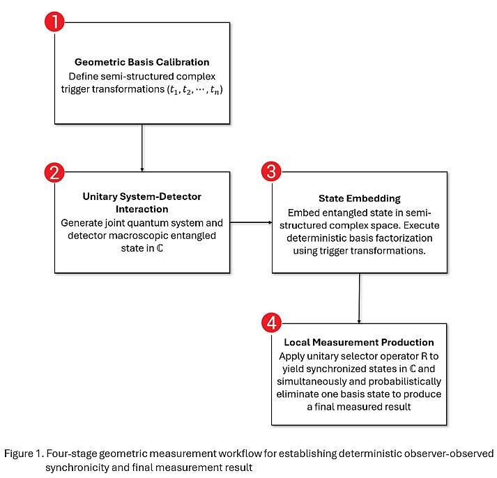
For the workflow Geometric Basis Calibration is achieved by defining the boundary conditions of the measurement interaction by defining the necessary number of orthogonal semi-structured complex trigger transformations () corresponding to the number of possible states of the quantum system that is to be measured.
Secondly, the Unitary System-Detector Interaction involves the target quantum state actively coupling with the macroscopic instrument via standard linear unitary evolution over the complex field , generating a correlated, entangled joint multipartite state [45,46].
Thirdly, the traditionally non-separable entangled state is embedded into semi-structured complex numbers state space. Utilizing the calibrated trigger transformations, the cross-term constraints involved in attempts to factorize entangled states are dealt with creating an explicit, non-arbitrary factorization of the joint state between the quantum system and detector.
Fourthly, a localized, single-subsystem restoration operator () is applied and has two functions. Firstly, to project the factorized representation back into standard Euclidean Hilbert space. Secondly, it uses the trigger transformations to cleanly remove the alternative state from both the particle and the detector. Instead of treating this choice as completely random, the model associates it with the structural weights of the two branches in the semi-structured space (Postulate 1, Section 3.0). This ensures that the final measurement reflects the structural properties of the original quantum system through an explicitly defined selection step rather than an unexplained random event.
3. Deterministic Wave Function Factorization for a Two-State System
To demonstrate the mathematical validity of this geometric factorization protocol, a general, two-state quantum system defined by the wave function shown in Equation (4) was analysed.

where represent arbitrary, complex probability amplitudes satisfying the strict normalization constraint . This quantum system is measured by a detector, and the measurement process consists of the following four steps:
Step 1: Geometric Basis Calibration (defining Trigger Transformations, their properties and relations)
The trigger transformations and are defined as projection operators acting on the semi-structured basis elements. It is important at this point to note that the detector apparatus is not defining these trigger transformations. They are defined from the amplitudes and of the quantum system itself (Equations (7) and (8)).
In semi-structured complex state space the operator projects components from the unstructured -axis (-domain) cleanly onto the real -axis within the -plane as shown in Equation (5).

Here is a real number. Note that the trigger transformation works equally well if was a complex number. However, if was a complex number operator would project components from the unstructured -axis (-domain) cleanly onto the complex -axis within the -plane.
Additionally, power on does not operate like regular exponential powers but simply indicates the power of the argument being projected from the unstructured -axis (-domain) cleanly onto the real -axis within the -plane.
Similarly, projects components from the imaginary unstructured -axis (-domain) onto the real -axis within the -plane:

Here is a real number. Note that the trigger transformation works equally well if was a complex number. However, if was a complex number operator would project components from the -axis (-domain) cleanly onto the complex -axis within the -plane.
Additionally, power on does not operate like regular exponential powers but simply indicates the power of the argument being projected from the unstructured -axis (-domain) cleanly onto the real -axis within the -plane.
By framing these transformations as projections, the vanishing of cross-terms () is a direct consequence of the mutual orthogonality of their domain spaces.
Equation (5) and Equation (6) can be written using shorthand notation as follows:

Equation (7) and Equation (8) does not mean are numbers. They are transformations. When evaluating for example , this means multiply the transformation and then evaluate the result (not evaluate individual results then multiply the evaluations). This is a shorthand algebraic proxy for the transformation mapping. These rules are stated formally in Appendix C (Definitions A3.3 and A3.4).
Step 2: Unitary System-Detector Interaction
Let the macroscopic detector be initialized to a stable, baseline “ready” pointer state denoted as . Define a standard, linear unitary measurement operator that governs the physical interaction between the quantum system and the detector at the point of contact [47,48]. For the detector to register the basis states faithfully, must satisfy the fundamental coupling criteria shown in Equation (9) and Equation (10) [49].

Because obeys strict linear dynamics over the standard complex field during the interaction between the detector and the arbitrary superposition state, applying to the arbitrary superposition state yields:

Substituting the foundational coupling criteria from Equations (9) and Equation (10) into this linear expansion generates the classic entangled joint state:

At this point, standard complex quantum mechanics encounters the measurement problem: the macroscopic apparatus is locked in a non-separable superposition with the quantum state, creating a macroscopic blur [50,51]. Step 3 and Step 4 address this problem within the extended framework.
Step 3: Factorizing entangled states using defined trigger transformations
To decouple this joint superposition deterministically, the state is mapped into semi-structured complex space. During this embedding, the traditionally vanishing cross-term amplitudes (the empty elements in Euclidean space) transform into non-zero auxiliary parameters and . Our objective is to factor the state which is and represent it in the form shown in Equation (13):

This implies that , , and . Embedding this entangled state into semi-structured complex state space means to simply transform 0 into a semi-structured complex number . From this point the following steps are taken:
Step A: Equate coefficients with constants

where are semi-structured complex numbers such that:

where and are semi-structured coefficients whose Euclidean projection back into standard complex Hilbert space vanishes; that is, in standard complex Hilbert space . Now consider the coefficients of and the coefficients of . These coefficients can be rewritten in terms of the trigger transformations. This is shown below:
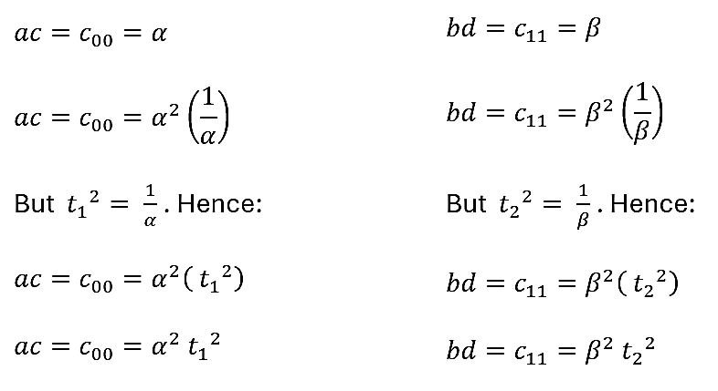
Hence, we have:

Step B: Get ratios r of the coefficients for each bracket in the factorization
To extract the relative ratios of the coefficients for each independent bracket within the factored tensor product, we establish the following:
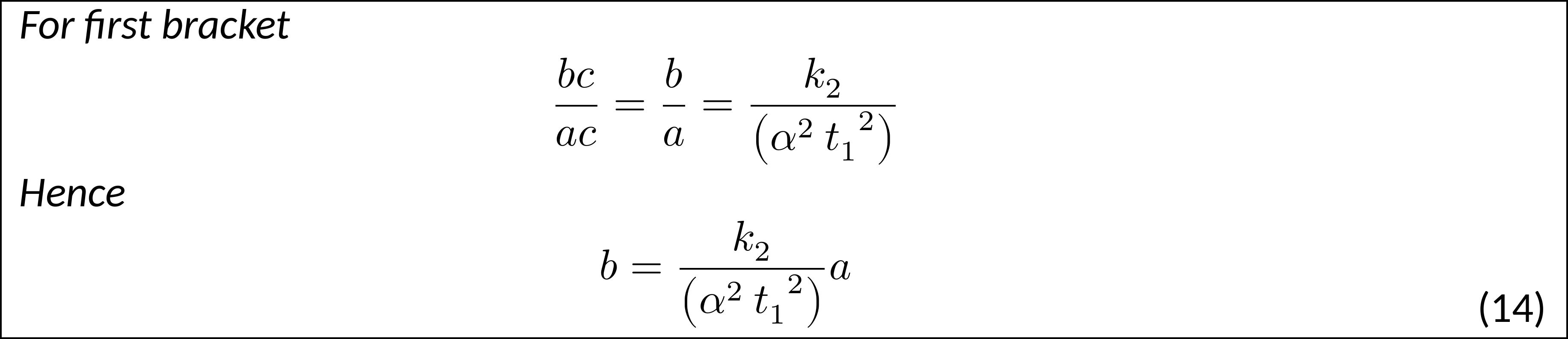
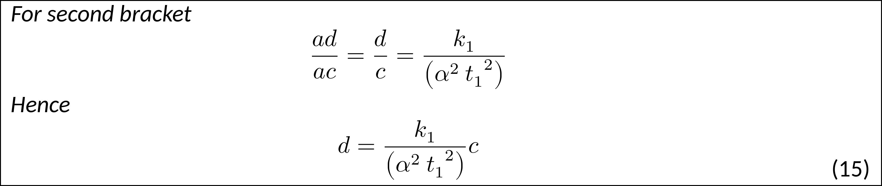
Step C: Setup Separability Conditions for factorization
The mandatory separability criterion governing independent bipartite systems is imposed to bind the auxiliary variables. For a two-state qubit system:

Substitute the coefficients of the equation and rearranging gives:

Step D: Solve simultaneous equations developed from Separability Conditions
There is only one equation (Equation (17)). Since there are two variables but only one equation this equation contains a free variable or under-determined degree of freedom. This implies that the value for one of the coefficients needs to be set. Set the values of the first coefficient such that . Solving under these conditions gives:
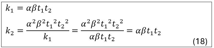
The choice for yields a perfectly mirrored value for the second parameter . Since under evaluation (Step 1), and are carried as unevaluated products during the factorization; this is precisely what ensures that they vanish on projection back to standard Hilbert space, as required in Step A.
Step E: Solve for the first coefficients
Given the general form , and where r is the ratio of coefficients, then the value of . Now also note:
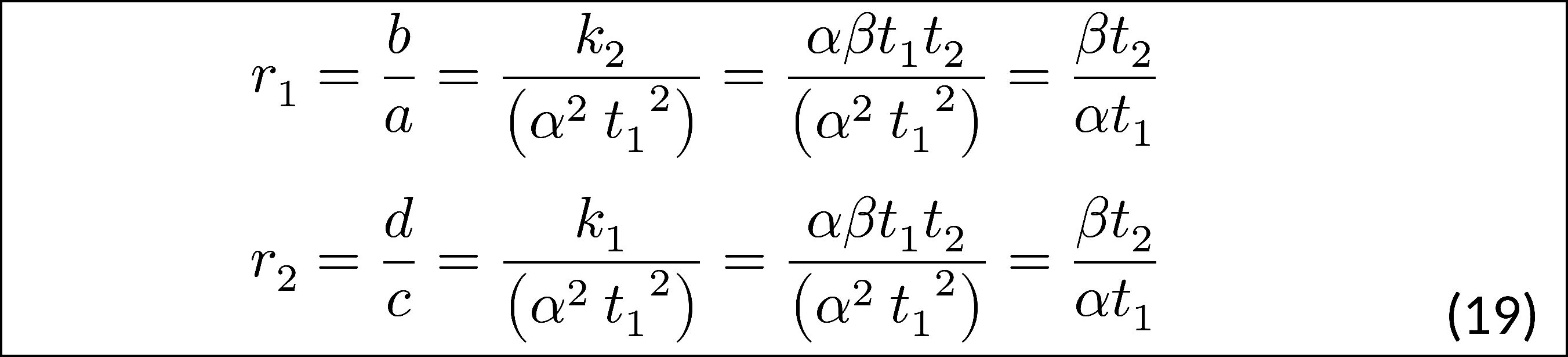
Also note that:
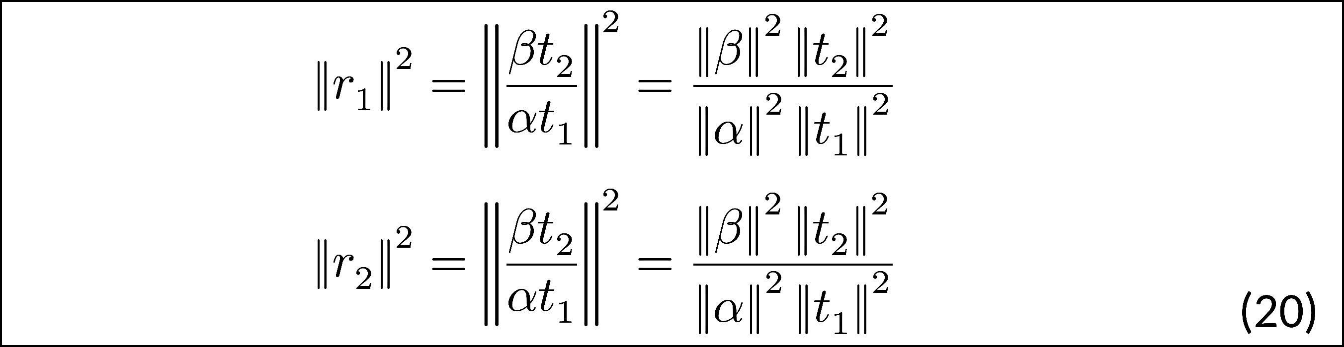
Hence using this gives the following for the factorized coefficients:
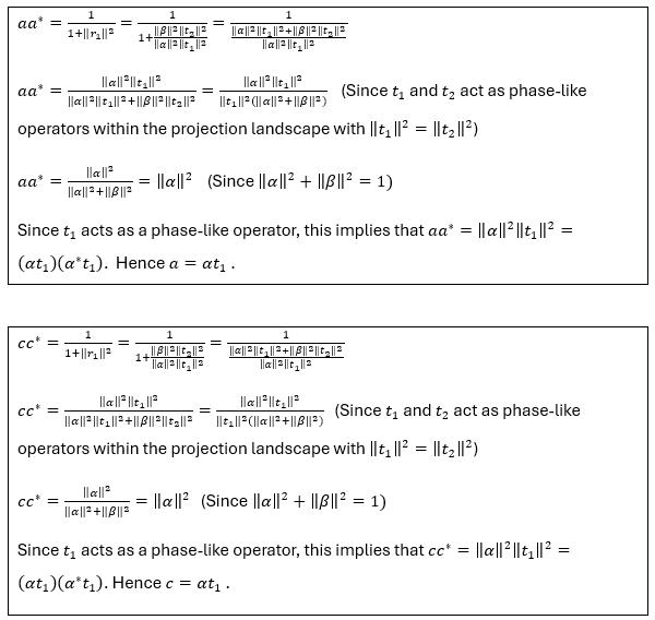
Confirming the choice of and .

Step F: Solve for the second coefficients
Using the equations from Step 2 and making the necessary substitutions gives:


This completes the deterministic factorization sequence of the entangled state within the semi-structured state space, mapping the entangled joint state (of the quantum system (sys) and detector (det)) into a perfectly decoupled, dual-perspective tensor product as shown in Equation (23).

Proposition 1 (Mirrored factorization). Let with , and let and obey the rules of Appendix C. Then, with the choice made in Step D, the joint state of Equation (12) is represented in semi-structured state space by the mirrored product of Equation (23), and evaluating this product with the rules of Appendix C returns Equation (12) exactly.
Proof. Expanding Equation (23) gives
Its coefficients are , , and , with , which are exactly the coefficients of Step A and satisfy the separability condition of Equations (16) and (17). Applying the evaluation rules of Appendix C (Definition A3.4) gives
so the evaluated state is , which is Equation (12). ∎
Remark. Equation (23) is therefore an equivalent representation of the joint state within the semi-structured space, not a physical disentanglement within . The factorization re-expresses the system–detector correlation in a form in which the two perspectives can be read separately, while remaining consistent with standard quantum mechanics on projection.
Step 4: Local Measurement Production
In Step 4, the trigger transformations and are treated as phase-like modulators (that is, operators intended to change the angle (phase) of a quantum state rather than its magnitude or probability) within the semi-structured state space; the conditions under which this holds are examined in Appendix B.
To return the decoupled states safely to standard Euclidean Hilbert space a selector operator constructed as the tensor product of two identical, single-subsystem local gates (represented as a matrix) is used as shown in Equation (24).

There are four important points to note about and how to construct . First, for any measurement there are “n” different types of , where “n” is the number of basis states that the quantum system being measured can be in. In this case, the quantum system being measured has two basis states . Hence there are two possible matrices . Note that each matrix has a subscript name that corresponded to the basis state; that is, matrices are name after the basis states. This is an important naming convention.
Secondly, the matrices are diagonal matrices with dimension , where “n” is the number of basis states that the quantum system being measured can be in. In this case, the quantum system being measured has two basis states , hence all matrices for this measurement are matrices.
Thirdly, all diagonal entries of the matrices is the trigger transformation that corresponds to the basis state it is named after. For example, is named after the first basis state, hence its diagonal entries are the trigger transformation attached to the first basis state; that is, , as shown in Equation (25). Similarly, is named after the second basis state, hence its diagonal entries are the trigger transformation attached to the second basis state; that is, , as shown in Equation (25).

Finally, each matrix or operator represents a distinct geometric branch into which the system can be selected. The standard quantum values and are interpreted here as the structural weights of the two branches, rather than as fundamental random odds. A branch is selected with probability equal to its structural weight, so the branch with the greater weight is proportionally more likely to be selected. In the present formulation, these weights and the resulting choice of selector enter the protocol as a postulate (Postulate 1, below); a dynamical derivation of the selection, and hence of the Born rule, is left for future work. This is shown in Result (26).
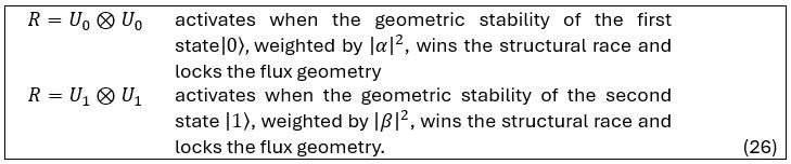
Postulate 1 (Branch selection). After the factorization of Step 3, exactly one selector is applied: with probability , or with probability . Result (26) gives the geometric interpretation of this rule; the rule itself is assumed, not derived, in the present model.
With this definition of the selector operator R and its component set , we can see how R acts on the tensor product produced by the factorization to yield the final measurement result. Hence, the outcome is determined by Equation (26).

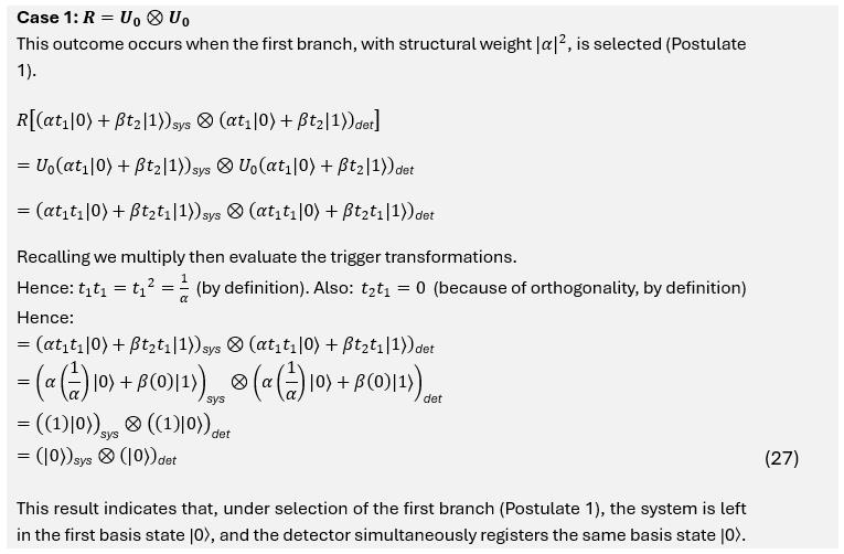
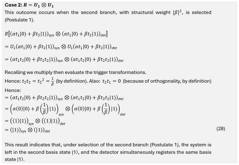
By applying the global operator to the entire decoupled tensor product, the strict linearity of quantum dynamics ensures simultaneous phase restoration across both reference frames and simultaneously produces a measurement result. To see how the measurement results are produced let us consider two cases, Case 1: and Case 2: as shown in Result (27) and Result (28) respectively.
Similarly,
Case 1 corresponds to selection of the first branch, which occurs with probability (Postulate 1). In this case, the quantum system is left in the first basis state , because the coefficient of the second basis state contains and therefore evaluates to zero. The detector also settles on the same basis state and registers this as a measurement.
There are two other points to note. Since the purpose of R was to move the factorized tensor product back to Hilbert space, the result or measurement in Case 1 occurs in Hilbert space with all the trigger transformations disappearing. Additionally, it is certain that the final measurement will be the first basis state as the coefficient of is 1 and the (certainty).
Similarly, Case 2 corresponds to selection of the second branch, which occurs with probability (Postulate 1). In this case, the quantum system is left in the second basis state , because the coefficient of the first basis state contains and therefore evaluates to zero. The detector also settles on the same basis state and registers this as a measurement.
There are two other points to note. Since the purpose of R was to move the factorized tensor product back to Hilbert space, the result or measurement in Case 2 occurs in Hilbert space with all the trigger transformations disappearing. Additionally, it is certain that the final measurement will be the second basis state as the coefficient of is 1 and the (certainty).
Hence Step 4 completes the measurement cycle. Based on this 4-step process, the selected outcome is a single basis state for both the system and the detector, and the outcome frequencies match the original structural weights of the quantum system being examined.
There is one more critical point to note. The selection described in Step 4 does not imply that the state with the larger geometric weight will be selected in every individual trial. In the quantum domain, the interaction zone is constantly influenced by microscopic, background vacuum fluctuations. In the interpretation adopted here, these fluctuations act as a perturbation of the selection step: although the branch with the larger weight is the more likely outcome, a fluctuation can lead to selection of the branch with the smaller weight, which then proceeds through the same selection step. This mechanism suggests that if an experimenter could artificially alter or direct these microscopic background fluctuations during the measurement window, it would theoretically change the final classical outcome. Consequently, if a coupling mechanism exists between these auxiliary geometric states and physical background vacuum fields, it could theoretically introduce a signature open to future experimental constraints. Therefore, the framework is deterministic once the microscopic fluctuation history is fixed, and is constructed to reproduce the statistical distributions observed in laboratory experiments over multiple trials.
4. Discussion
4.1. Foundational Insight: The Synchronicity Chain
The application of this 4-step geometric protocol to a bipartite system provides an alternative to traditional interpretations of quantum mechanics [52,53]. In standard quantum mechanics over the complex field ℂ, the interaction between a quantum system and a macroscopic measuring apparatus creates an entangled state that cannot be separated. From this perspective it is impossible to evaluate the system or the detector as independent, localized entities [54].
The introduction of semi-structured complex algebra offers a way around this mathematical bottleneck. Step 3 and Step 4 in the proposed factorization protocol function as an algebraic coordinator that represents the traditionally non-separable entangled wave function, within the semi-structured space, as a product of two mirrored factors; one representing how the quantum system behaves and the other representing how the detector registers the quantum system.
Although written as separate factors, the structural coefficients (of each subsystem) ensure that the subsystems correlation remain mathematically locked. Step 3 ensures that the measuring apparatus frame and the target quantum system's frame are perfectly mirrored. When a macroscopic observer interacts with the measuring apparatus, they do not trigger a wave function collapse. Instead, the system and the detector remain synchronized through the mirrored factorization of Step 3. The interaction is then completed by the selection step of Step 4 (the geometric freezing event, in the interpretive language of this paper), in which one branch is retained with probability equal to its structural weight (Postulate 1). This toy model offers a structural alternative to the mystery of an instantaneous, random wave function collapse, proposing an orderly, explicitly defined selection process that leaves a single, definite outcome.
In Step 4 the tensor product is returned to Hilbert space using a selector operator R (consisting of a tensor product of operators whose entries are trigger transformations). It is this R that helps produce the final measured result in Hilbert space and, within the model, removes the need to assume that the macroscopic detector must be in some quantum blur because of its entanglement with the microscopic quantum system.
4.2. Environmental Imprinting of Quantum State's Structural Properties
Within Step 3 of the proposed protocol, a quantum measurement process partly consists of the deterministic imprinting of a microscopic quantum state's structural properties onto the macroscopic detector. Traditional measurement models assume that any interaction with an external apparatus is fundamentally destructive, causing the immediate decay of the initial state superposition [55].
The geometric protocol presented here demonstrates a non-destructive alternative. By initializing the system at alongside a baseline detector state , the total evolution yields the decoupled product:

Within the model, this result indicates that the detector’s factor carries the same structural coefficients as the quantum system’s factor, without an arbitrary collapse. In this representation, the macroscopic environment mirrors the quantum system. This suggests a mathematical picture of how subatomic information can be amplified into the macroscopic domain while preserving its structural coherence [56,57]. Equation (29) should be read as shorthand for the factorized form of Equation (23), with the trigger transformations suppressed; it is not a copy of the state within standard Hilbert space, which the no-cloning theorem forbids for unitary dynamics. On projection back to , the product form coincides with the entangled state of Equation (12). It is only the natural selector operator R that reduces the wave functions of the quantum system and the detector to a single value.
4.3. Reframing the Role of Non-Unitary Wave Function Collapse
The Von Neumann-Wigner interpretation historically assumed that a measurement event must result in a non-unitary, wave function collapse [58]. This is because standard Hilbert space geometry offers no pathway to separate the cross-terms of an entangled state like . By routing the entangled joint state through an intermediate embedding in semi-structured complex space, this protocol offers a way to replace an ad-hoc collapse postulate with an explicitly defined selection step.
This reframing rests on three specific geometric properties. First, the protocol suggests that the entangled “stalemate” is an artifact of the rigid dimensionality of standard complex numbers. Secondly, the protocol demonstrates that the target state and the macroscopic apparatus can be represented as separate, mirrored factors within the semi-structured space ( and ). Additionally, the protocol confirms that both subsystems maintain identical, stable quantum profiles throughout the factorization stage, so that the elimination of an alternative eigenstate occurs only at a single, explicitly defined point: the action of the selection operator R (see Appendix B).
It is important to clarify the mathematical nature of the trigger transformations and in Equations (7) and (8). Because these transformations depend directly on the specific values of and , they introduce a deliberate, non-linear element to the framework during the intermediate math phase. In standard quantum mechanics, measuring tools (operators) are strictly separated from the things they measure (states). However, in this model, the unobservable extended state space describes an active, context-dependent physical environment. In particular, the rules of the extended space depend on the state being measured, so that the internal weights of the system enter the measurement step directly. This state dependence is also what allows the calculation to avoid indeterminate expressions such as division by zero. This places the model alongside other non-linear proposals, such as Weinberg’s non-linear quantum mechanics and objective collapse theories, and it inherits their central constraint: non-linear state dependence can, in general, permit superluminal signalling [59,60]. Here the state dependence is confined to the unobservable intermediate stage; showing that it produces no signalling at the physical endpoints is an important open question. The model thus suggests that standard linear rules may be simplified approximations of a richer, state-dependent geometric structure.
4.4. Implications for the Wigner’s Friend Paradox
The Wigner’s Friend paradox is a contradiction in quantum mechanics where an observer inside an isolated laboratory (the Friend) records a definite macroscopic outcome, while an external observer (Wigner) describes the entire laboratory as an un-collapsed, entangled macro-superposition [61,62]. The protocol developed here suggests a possible reading of this scenario, which we outline briefly.
In the model, the Friend’s measurement corresponds to the factorization of Step 3, which represents the Friend’s apparatus and the particle as mirrored factors within the semi-structured space. Wigner’s description of the laboratory corresponds to the same state viewed in standard Hilbert space where, by Proposition 1, it remains the entangled state of Equation (12). A definite outcome arises for either observer only through the selection step of Postulate 1. Whether this assignment of perspectives is consistent with recent local-friendliness no-go results requires a detailed analysis, which is left for future work [63].
5. Conclusion
In standard complex quantum mechanics, the measurement problem arises because a macroscopic detector is forced into an entangled state with the target quantum state, providing no linear mathematical explanation for why a single, stable classical reality is observed. This paper proposes a geometric toy model of this problem, with a deterministic factorization stage and a postulated selection step, through a 4-step measurement protocol that embeds the joint entangled state of the quantum system and the detector into semi-structured complex state space.
By introducing localized projection operators defined as trigger transformations, the paper proposes a structured protocol that creates an explicit, non-arbitrary factorization of the entangled joint state into two identical independent subsystems within the semi-structured state space, a representation that reduces to the original entangled state on projection back to standard Hilbert space. This algorithm maps the initial system comprising of a quantum subsystem and a blank detector directly into a synchronized tensor product state, written in the shorthand of Equation (29) as . This protocol effectively imprints the structural properties of the quantum superposition onto the macroscopic environment, so that, in this representation, the apparatus mirrors the quantum subsystem. The generation of the synchronized output states indicates that, within the model, the observer's frame of reference is aligned with the objective behaviour of the quantum system.
The protocol then applies a selection operator R to this synchronized tensor product to produce the final measurement result in Hilbert space. Rather than an unexplained random collapse, the operator R implements the selection step, which in the interpretive language of this paper corresponds to the topological phase transition. The final classical value is the branch selected according to Postulate 1. By interpreting standard probabilities as structural weights, the framework links the final unique outcome directly to the internal stability of the original quantum system.
This extended algebraic architecture provides a formal method for wave function factorization that reframes non-unitary wave function collapse as a single, explicitly defined selection step, modelling quantum measurement as a deterministic factorization in an extended geometric space followed by that postulated selection. Two questions remain open for future work: deriving the selection dynamics, and with them the Born weights, from first principles; and constructing a fully unitary realization of the selector R that excludes superluminal signalling at the physical endpoints.
Funding
The authors received no specific funding for this work.
Ethics approval
This article does not contain any studies involving human participants or animals performed by any of the authors. Ethics approval is therefore not applicable.
Competing interests
The authors declare that they have no competing interests.
Data availability
Data sharing is not applicable to this article as no datasets were generated or analysed during the current study. All results reported are derived analytically and are fully reproducible from the equations and derivations presented in the manuscript and its appendices.
Appendix A. Original Algorithm for Factorizing Entangled States
This appendix presents the original algorithm for factorizing entangled states and then provides a critique of the weakness of the algorithm and why (with some modification) it is still good as a foundational algorithm for factoring entangled states.
PART 1: ORIGINAL ALGORITHM
Algebraic Foundations and Transformation Rules
Let be a standard complex Hilbert space spanned by the computational basis . To construct the extended semi-structured space , we establish an algebraic structure mediated by an auxiliary symbol and parameter variables governed by four precise transformation axioms:
- 1.
- The Extended Map: The standard Euclidean value maps to a non-zero auxiliary form in semi-structured space:

- 2.
- The Inverse Projection: The physical mapping back to the standard domain cleanly annihilates the auxiliary element:

- 3.
- The -Conjugate: Conjugation inside the semi-structured space handles real and imaginary parameter matrices according to the rule:

- 4.
- The Trigger Transformation: Indeterminate divisions caused by vanishing parameters are assigned, by convention, a state-dependent, regularized real constant

In standard arithmetic, dividing zero by zero is impossible and breaks down. In the original algorithm, Axiom 4 therefore acts as a regularization rule, analogous to a gauge-fixing choice: the indeterminate ratio is replaced by a value fixed by the state. The resulting value, , is not a random guess; it is determined by the state’s coefficients. As discussed in Part 2, giving this rule a rigorous foundation remains an open task.
2.2 Generalized Factorization Algorithm
The algorithm to reduce an entangled state to an independent tensor product operates through a sequential six-step protocol:
Figure A1.
Generalized Factorization Workflow.
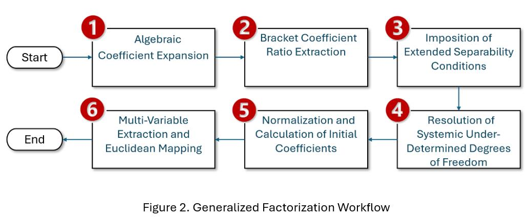
Step 1: Coefficient Expansion
The target non-separable entangled multipartite state vector is equated to a general, hypothetical tensor product of localized single-qubit states. For a general bipartite system, this takes the form:

The known constants are written, while the traditionally vanishing entries (that is, states that have the coefficient equal to zero) are mapped to auxiliary variables,

Step 2: Bracket Coefficient Ratio Extraction
Use the expanded state coefficients to find the ratio of the coefficients in each bracket:

This yields immediate dependencies, rephrasing output coefficients directly in terms of base states (e.g., ).
Step 3: Solving for auxiliary parameters using Separability Condition to create simultaneous equation(s)
Use the separability condition to find the value of auxiliary variables . The separability condition for the Bell States is . Substituting the constants and auxiliary variables into this relation forms the central bounding equation of the method.
Step 4: Resolution of Systemic Under-Determined Degrees of Freedom
Because the resulting system of equations from Step 3 possesses fewer constraints than variables, a free variable selection is made for the first unknown essentially setting up constraint conditions. Therefore let:

where . Solving the algebraic equations from Step 3 under these specific settings yields closed expressions or solutions for all remaining auxiliary variables.
Step 5: Normalization and Calculation of Initial Coefficients
Using Equation (9) the first coefficient of each bracket of the tensor product is calculated using the ratios found in Step 2. This exploits the fact that coefficients the squared norm of the coefficients of each bracket must add to 1.

Step 6: Solving for the remaining coefficients and inverse Euclidean Mapping
With the initial base coefficients confirmed, the remaining variables () are directly computed via back-substitution into the ratio identities shown in Step 2. The resulting expressions represent a perfect factorization of the Bell States in semi-structured complex space. Applying the final inverse operator to the product of the factorized brackets ensuring smooth transformation back to the original quantum measurements for the Bell States.
PART 2: CRITIQUE OF ALGORITHM
Whilst the generalized six-step factorization protocol outlined in Appendix A provides a powerful and innovative starting blueprint for state separation, a rigorous mathematical audit reveals specific foundational boundaries that require further development.
- Step 4 relies heavily on evaluating indeterminate expressions. In standard linear algebra over a complex field, operations mimicking division by zero are strictly undefined. While this framework regularizes these points as local gauge-fixing parameters to make the factorization functional, treating them as simple real constants without an explicit topological foundation introduces potential structural fragility to the baseline axioms.
- 2.
- During Step 3, transforming traditionally empty Euclidean cross-term elements into non-zero auxiliary semi-structured numbers technically modifies the original wave function's profile. Because these parameters vanish when projected back to standard Hilbert space, the physical state is preserved at the endpoints; however, during the intermediate factorization phase, the algorithm operates on an extended mathematical state space rather than the isolated, authentic quantum state. More work needed to be done to show why this should occur.
Highlighting these two critiques does not diminish the algorithm’s utility. Instead, it explicitly justifies why the model must evolve from simple algebraic substitution toward the selection mechanism described in the main body of this text. By treating the algorithm as an approximation of this mechanism, future work can completely justify the use of these algebraic proxies.
Appendix B. Mathematical Proof of Conditions for a Unitary Operator R
The existence of a global, state-independent unitary selector operator that successfully maps the decoupled semi-structured state back into Euclidean space requires that the trigger transformations and belong strictly to the group of unimodular phase modulators (i.e., ). This constraint would guarantee that the operator strictly preserves the inner product across all arbitrary superpositions, thereby maintaining foundational quantum linearity and compliance with the evolution postulates within the physical endpoints of the Hilbert space field .
In quantum mechanics, a fundamental property of any unitary operator is that it must be linear and preserve the inner product (overlap) between any two states. We can prove whether exists by testing this property.
The Mathematical Proof
We define the starting state as and the target state (with and removed) as :

For a single unitary operator to exist such that for any choice of amplitudes, it must preserve the inner product between two different states, say picking coefficients and a different set . Therefore, it must satisfy:

- Calculate the Target Overlap

- 2.
- Calculate the Initial Overlap

3. The Condition for Unity
For these two overlaps to be equal for all arbitrary values of , the coefficients inside the parentheses must match exactly. This forces:

Comparing Equation (42) with Equation (7), which gives , shows that the unimodular condition can hold only when (and likewise for ), that is, only in the absence of superposition. For a genuine superposition, therefore, cannot be realized as a single, state-independent unitary operator. In the present model, is accordingly interpreted as a branch-selecting map: each choice, or , projects onto one branch, so that the evolution is unitary up to the point of selection and the non-unitary step is confined to itself. Constructing a fully unitary realization of , for example by explicitly including the environment, is left for future work.
Appendix C. Formal Definitions of the Semi-Structured and Trigger Algebras
This appendix collects the algebraic rules used in the main body, so that every calculation in Section 1.4 and Section 3.0 can be checked directly against them.
Definition A3.1 (Semi-structured complex numbers). The set consists of the numbers with . Addition and multiplication by real scalars are carried out component by component, and the imaginary unit satisfies . The complex numbers form the subset with .
Definition A3.2 (Powers of the unstructured unit). The unstructured unit satisfies
and, in general, , so the powers of repeat with period 4.
Remark A3.2a. If, in addition, and are taken to commute, then , so that behaves as a hyperbolic unit and the multiplication of coincides with that of the bicomplex numbers [64]. Under this assumption, the elements below are orthogonal idempotents:
This orthogonal-idempotent structure is the algebraic counterpart of the orthogonality relation used for the trigger transformations below.
Definition A3.3 (Trigger transformations). For a state with amplitudes , the trigger transformations and are formal symbols that act only within semi-structured state space: projects the -domain onto the real axis (Equations (2) and (5)), and projects the -domain onto the real axis (Equation (6)). They commute with each other and with scalar coefficients. Products of trigger transformations are formed first and evaluated afterwards (Section 3.0, Step 1).
Definition A3.4 (Evaluation rules). The evaluation map returns an expression in trigger transformations to an ordinary complex number. On single symbols and their powers it acts as
for . Thus , , , and so on, with the corresponding rules for . These are Equations (7) and (8) together with the orthogonality relation . The map is extended linearly: for scalar coefficients and products of trigger transformations .
Remark A3.4a. The map is linear but not multiplicative: , whereas . This is why products must be formed before they are evaluated, and why and cannot be replaced by numbers before evaluation. Applied to the coefficients of a state, plays the role of the projection back to standard Hilbert space: the auxiliary parameters of Step A evaluate to zero, as required, while and evaluate to and (Proposition 1).
References
- Hance, J. R.; Hossenfelder, S. What does it take to solve the measurement problem? J. Phys. Commun. 2022, vol. 6(no. 10), Art. no. 102001. [Google Scholar] [CrossRef]
- Bassi; Dorato, M.; Ulbricht, H. Collapse models: A theoretical, experimental and philosophical review. Entropy 2023, vol. 25(no. 4), Art. no. 645. [Google Scholar] [CrossRef] [PubMed]
- Schonfeld, J. F. Measured distribution of cloud chamber tracks from radioactive decay: A new empirical approach to investigating the quantum measurement problem. Open Phys. 2022, vol. 20(no. 1), 40–48. [Google Scholar] [CrossRef]
- Schonfeld, J. F. Does the Mott problem extend to Geiger counters? Open Phys. 2023, vol. 21(no. 1). [Google Scholar] [CrossRef]
- Żukowski, M.; Markiewicz, M. Physics and metaphysics of Wigner’s friends: Even performed premeasurements have no results. Phys. Rev. Lett. 2021, vol. 126(no. 13), Art. no. 130402. [Google Scholar] [CrossRef] [PubMed]
- Zurek, W. H. Quantum theory of the classical: Einselection, envariance, quantum Darwinism and extantons. Entropy 2022, vol. 24(no. 11), Art. no. 1520. [Google Scholar] [CrossRef] [PubMed]
- Donadi, S.; Hossenfelder, S. Toy model for local and deterministic wave-function collapse. Phys. Rev. A 2022, vol. 106(no. 2), Art. no. 022212. [Google Scholar] [CrossRef]
- Tomaz; Mattos, R. S.; Barbatti, M. Gravitationally-induced wave function collapse time for molecules. Phys. Chem. Chem. Phys. 2024, vol. 26(no. 31), 20785–20798. [Google Scholar] [CrossRef] [PubMed]
- Renou, M.-O.; et al. Quantum theory based on real numbers can be experimentally falsified. Nature 2021, vol. 600(no. 7890), 625–629. [Google Scholar] [CrossRef] [PubMed]
- Gisin, N. Indeterminism in physics, classical chaos and Bohmian mechanics: Are real numbers really real? Erkenntnis 2021, vol. 86(no. 6), 1469–1481. [Google Scholar] [CrossRef]
- Kofman, G.; Kurizki, G. Does decoherence select the pointer basis of a quantum meter? Entropy 2022, vol. 24(no. 1), Art. no. 106. [Google Scholar] [CrossRef] [PubMed]
- Di Biagio; Rovelli, C. Stable facts, relative facts. Found. Phys. 2021, vol. 51(no. 1, Art. no. 30). [Google Scholar] [CrossRef]
- Robson. Relational quantum mechanics and contextuality. Found. Phys. 2024, vol. 54(no. 4, Art. no. 54). [Google Scholar] [CrossRef]
- Ollivier, H. Emergence of objectivity for quantum many-body systems. Entropy 2022, vol. 24(no. 2), Art. no. 277. [Google Scholar] [CrossRef] [PubMed]
- Giacomini, F.; Brukner, Č. Quantum superposition of spacetimes obeys Einstein’s equivalence principle. AVS Quantum Sci. 2022, vol. 4(no. 1), Art. no. 015601. [Google Scholar] [CrossRef]
- Çakmak; Müstecaplıoğlu, Ö. E.; Paternostro, M.; Vacchini, B.; Campbell, S. Quantum Darwinism in a composite system: Objectivity versus classicality. Entropy 2021, vol. 23(no. 8), Art. no. 995. [Google Scholar] [CrossRef] [PubMed]
- Mirkin, N.; Wisniacki, D. A. Many-body localization and the emergence of quantum Darwinism. Entropy 2021, vol. 23(no. 11), Art. no. 1377. [Google Scholar] [CrossRef] [PubMed]
- Le, T. P.; Winter, A.; Adesso, G. Thermality versus objectivity: Can they peacefully coexist? Entropy 2021, vol. 23(no. 11), Art. no. 1506. [Google Scholar] [CrossRef] [PubMed]
- García-Pintos, L. P.; del Campo, A. Limits to perception by quantum monitoring with finite efficiency. Entropy 2021, vol. 23(no. 11), Art. no. 1527. [Google Scholar] [CrossRef] [PubMed]
- Li, Z.-D.; et al. Testing real quantum theory in an optical quantum network. Phys. Rev. Lett. 2022, vol. 128(no. 4), Art. no. 040402. [Google Scholar] [CrossRef] [PubMed]
- Chen, M.-C.; et al. Ruling out real-valued standard formalism of quantum theory. Phys. Rev. Lett. 2022, vol. 128(no. 4), Art. no. 040403. [Google Scholar] [CrossRef] [PubMed]
- Wu, et al. Experimental refutation of real-valued quantum mechanics under strict locality conditions. Phys. Rev. Lett. 2022, vol. 129(no. 14), Art. no. 140401. [Google Scholar] [CrossRef] [PubMed]
- Braasch, W. F., Jr.; Wootters, W. K. A classical formulation of quantum theory? Entropy 2022, vol. 24(no. 1), Art. no. 137. [Google Scholar] [CrossRef] [PubMed]
- Saruhan, İ.; von Zanthier, J.; Pleinert, M.-O. Multipath and multiparticle tests of complex versus hypercomplex quantum theory. Phys. Rev. Lett. vol. 134(no. 6), Art. no. 060201, 2025. [CrossRef] [PubMed]
- Secgin; Ilguz, C. R.; Gok, I. On complex hybrid numbers: Algebraic structures, matrix representations, and geometric interpretations. Kuwait J. Sci. 2026, vol. 53(no. 1), Art. no. 100528. [Google Scholar] [CrossRef]
- Jean-Paul, P.; Wahid, S. Unstructured and semi-structured complex numbers: A solution to division by zero. Pure Appl. Math. J. 2021, vol. 10(no. 2), 49–61. [Google Scholar] [CrossRef]
- Bergstra, J. A.; Tucker, J. V. Logical models of mathematical texts II: Legality conventions for division by zero in inconsistent contexts. J. Log. Lang. Inf. 2025. [Google Scholar] [CrossRef]
- Jean-Paul, P.; Wahid, S. Reformulating and strengthening the theoretical foundations of semi-structured complex numbers. Int. J. Appl. Phys. Math. 2022, vol. 12(no. 4), 34–58. [Google Scholar] [CrossRef]
- Jean-Paul, P.; Wahid, S. Complete factorization of entangled quantum states PART 1: Factorizing the Bell states using semi-structured complex numbers. Preprints 2026. [Google Scholar] [CrossRef]
- Jean-Paul, P.; Wahid, S. Complete factorization of entangled quantum states PART 2: Factorizing the GHZn and W states using semi-structured complex numbers. Preprints 2026. [Google Scholar] [CrossRef]
- Hubert, M. Is the statistical interpretation of quantum mechanics ψ-ontic or ψ-epistemic? Found. Phys. 2023, vol. 53(no. 1, Art. no. 16). [Google Scholar] [CrossRef]
- Ney. Three arguments for wave function realism. Eur. J. Philos. Sci. 2023, vol. 13(no. 4, Art. no. 50). [Google Scholar] [CrossRef]
- Donadi, S.; Piscicchia, K.; Curceanu, C.; Diósi, L.; Laubenstein, M.; Bassi, A. Underground test of gravity-related wave function collapse. Nat. Phys. 2021, vol. 17(no. 1), 74–78. [Google Scholar] [CrossRef]
- Arnquist, J.; et al. Search for spontaneous radiation from wave function collapse in the Majorana Demonstrator. Phys. Rev. Lett. 2022, vol. 129(no. 8), Art. no. 080401. [Google Scholar] [CrossRef] [PubMed]
- Oppenheim, J. A postquantum theory of classical gravity? Phys. Rev. X 2023, vol. 13(no. 4), Art. no. 041040. [Google Scholar] [CrossRef]
- Oppenheim, J.; Sparaciari, C.; Šoda, B.; Weller-Davies, Z. Objective trajectories in hybrid classical-quantum dynamics. Quantum 2023, vol. 7, Art.(no. 891). [Google Scholar] [CrossRef]
- Sutherland, R. I. Probabilities and certainties within a causally symmetric model. Found. Phys. 2022, vol. 52(no. 4, Art. no. 75). [Google Scholar] [CrossRef]
- Ridley, M.; Adlam, E. Time and event symmetry in quantum mechanics. Quantum Stud. Math. Found. 2025, vol. 12(no. 1, Art. no. 9). [Google Scholar] [CrossRef]
- Fu, S.; Luo, S. Quantifying decoherence via increases in classicality. Entropy 2021, vol. 23(no. 12), Art. no. 1594. [Google Scholar] [CrossRef] [PubMed]
- Auffèves; Grangier, P. Revisiting Born’s rule through Uhlhorn’s and Gleason’s theorems. Entropy 2022, vol. 24(no. 2), Art. no. 199. [Google Scholar] [CrossRef] [PubMed]
- Mironowicz, P.; Horodecki, P.; Horodecki, R. Non-perfect propagation of information to a noisy environment with self-evolution. Entropy 2022, vol. 24(no. 4, Art. no. 467). [Google Scholar] [CrossRef] [PubMed]
- Drezet. Justifying Born’s rule Pα = |Ψα|² using deterministic chaos, decoherence, and the de Broglie–Bohm quantum theory. Entropy 2021, vol. 23(no. 11), Art. no. 1371. [Google Scholar] [CrossRef] [PubMed]
- Short, J. Probability in many-worlds theories. Quantum 2023, vol. 7, Art.(no. 971). [Google Scholar] [CrossRef]
- Carroll, S. M.; Lodman, J. Energy non-conservation in quantum mechanics. Found. Phys. 2021, vol. 51(no. 4), Art. no. 83. [Google Scholar] [CrossRef]
- Wu, W.; Scholes, G. D. Foundations of quantum information for physical chemistry. J. Phys. Chem. Lett. 2024, vol. 15(no. 15), 4056–4069. [Google Scholar] [CrossRef] [PubMed]
- Spegel-Lexne, D.; et al. Experimental demonstration of the equivalence of entropic uncertainty with wave-particle duality. Sci. Adv. 2024, vol. 10(no. 49), Art. no. eadr2007. [Google Scholar] [CrossRef] [PubMed]
- Polo-Gómez, J.; Garay, L. J.; Martín-Martínez, E. A detector-based measurement theory for quantum field theory. Phys. Rev. D. 2022, vol. 105(no. 6), Art. no. 065003. [Google Scholar] [CrossRef]
- Bostelmann; Fewster, C. J.; Ruep, M. H. Impossible measurements require impossible apparatus. Phys. Rev. D. 2021, vol. 103(no. 2), Art. no. 025017. [Google Scholar] [CrossRef]
- Gisin, N.; Del Santo, F. Towards a measurement theory in QFT: Impossible quantum measurements are possible but not ideal. Quantum 2024, vol. 8, Art.(no. 1267). [Google Scholar] [CrossRef]
- Kaufman; Marquetand, P.; Rozgonyi, T.; Weinacht, T. Long-lived electronic coherences in molecules. Phys. Rev. Lett. 2023, vol. 131(no. 26), Art. no. 263202. [Google Scholar] [CrossRef] [PubMed]
- Shu, Y.; Truhlar, D. G. Decoherence and its role in electronically nonadiabatic dynamics. J. Chem. Theory Comput. 2023, vol. 19(no. 2), 380–395. [Google Scholar] [CrossRef] [PubMed]
- Khrennikov. Ozawa’s intersubjectivity theorem as objection to QBism individual agent perspective. Int. J. Theor. Phys. 2024, vol. 63(no. 1, Art. no. 23). [Google Scholar] [CrossRef]
- Khrennikov. Relational quantum mechanics: Ozawa’s intersubjectivity theorem as justification of the postulate on internally consistent descriptions. Found. Phys. 2024, vol. 54(no. 3, Art. no. 29). [Google Scholar] [CrossRef]
- Oaknin, H. Bypassing the Kochen–Specker theorem: An explicit non-contextual statistical model for the qutrit. Axioms 2023, vol. 12(no. 1, Art. no. 90). [Google Scholar] [CrossRef]
- Costello, J. B.; et al. Reconstruction of Bloch wavefunctions of holes in a semiconductor. Nature 2021, vol. 599(no. 7883), 57–61. [Google Scholar] [CrossRef] [PubMed]
- Zwolak, M. Amplification, inference, and the manifestation of objective classical information. Entropy 2022, vol. 24(no. 6), Art. no. 781. [Google Scholar] [CrossRef] [PubMed]
- Taylor, J. K.; McCulloch, I. P. Wavefunction branching: When you can’t tell pure states from mixed states. Quantum vol. 9, Art.(no. 1670), 2025. [CrossRef]
- Oppenheim, J.; Sparaciari, C.; Šoda, B.; Weller-Davies, Z. Gravitationally induced decoherence vs space-time diffusion: Testing the quantum nature of gravity. Nat. Commun. 2023, vol. 14(no. 1), Art. no. 7910. [Google Scholar] [CrossRef] [PubMed]
- Gisin, N. Weinberg’s non-linear quantum mechanics and supraluminal communications. Phys. Lett. A 1990, vol. 143(no. 1–2), 1–2. [Google Scholar] [CrossRef]
- Polchinski, J. Weinberg’s nonlinear quantum mechanics and the Einstein–Podolsky–Rosen paradox. Phys. Rev. Lett. 1991, vol. 66(no. 4), 397–400. [Google Scholar] [CrossRef] [PubMed]
- Wiseman, M.; Cavalcanti, E. G.; Rieffel, E. G. A thoughtful local friendliness no-go theorem: A prospective experiment with new assumptions to suit. Quantum 2023, vol. 7, Art.(no. 1112). [Google Scholar] [CrossRef]
- Cavalcanti, G.; Wiseman, H. M. Implications of local friendliness violation for quantum causality. Entropy 2021, vol. 23(no. 8), Art. no. 925. [Google Scholar] [CrossRef] [PubMed]
- Zeng, W. J.; Labib, F.; Russo, V. Towards violations of local friendliness with quantum computers. Quantum vol. 9, Art.(no. 1851), 2025. [CrossRef]
- G. B. Price, An Introduction to Multicomplex Spaces and Functions; Marcel Dekker: New York, NY, USA, 1991.
Disclaimer/Publisher’s Note: The statements, opinions and data contained in all publications are solely those of the individual author(s) and contributor(s) and not of MDPI and/or the editor(s). MDPI and/or the editor(s) disclaim responsibility for any injury to people or property resulting from any ideas, methods, instructions or products referred to in the content. |
© 2026 by the authors. Licensee MDPI, Basel, Switzerland. This article is an open access article distributed under the terms and conditions of the Creative Commons Attribution (CC BY) license (http://creativecommons.org/licenses/by/4.0/).
Copyright: This open access article is published under a Creative Commons CC BY 4.0 license, which permit the free download, distribution, and reuse, provided that the author and preprint are cited in any reuse.