

Submitted:
09 October 2026
Posted:
12 October 2026
You are already at the latest version
Abstract
Forests worldwide face intensifying natural and anthropogenic pressures that progressively erode their resilience, bringing them closer to abrupt, potentially irreversible shifts. Such loss of resilience can manifest as critical slowing down (CSD), a phenomenon characterized by slower recovery rates. It is often measured through statistical indicators, known as early warning signals, which are expected to rise in advance of a critical transition such as a tipping point. Earth Observation (EO) is well suited to monitoring CSD indicators at global scales. However, the reliability of these indicators depends strongly on the quality and consistency of the underlying satellite record given their derivation from optical biophysical proxies. This is particularly true for what is arguably one of the most useful EO dataset – the Landsat Collection 2 archive, given its extensive temporal coverage (1984-present) and 30-m spatial resolution. Here, we present a scalable and reproducible workflow for generating high-quality, long-term, cross-calibrated Landsat datasets specifically designed for the computation of statistical indicators of resilience over large extents of forest ecosystems. The workflow integrates robust imagery processing, consistent radiometric cross-calibration, and a multiscale grid-based implementation to improve the reliability of the Landsat imagery used for resilience analysis. Using an undisturbed boreal forest region in Quebec, Canada, as a case study, we demonstrate that the proposed workflow reduces inter-sensor discontinuities, enhances spatial consistency and preserves ecologically meaningful temporal dynamics across the 40-year Landsat record. Applied across ecoregions and biomes, this framework seeks to enable robust and comparable assessments of forest resilience, supporting large-scale ecosystem monitoring, early-warning assessments, and evidence-based conservation prioritisation.
Keywords:
resilience
; early warning signals
; tipping points
; Landsat
; forests
; boreal
1. Introduction
Global forests are increasingly threatened by climate and land-use changes across biomes (McDowell et al., 2020) that progressively erode their capacity to recover after disturbances (Li et al., 2018; Pimm, 1984). This loss of resilience manifests as critical slowing down (CSD), a phenomenon characterized by slower recovery rates, often measured through statistical indicators (Dakos et al., 2008). CSD-based metrics like variance, autocorrelation and skewness are expected to increase in proximity to a critical transition, or regime shift (Bathiany et al., 2025; Scheffer et al., 2015, 2009). These indicators, known as early warning signals (EWS), were originally derived from theoretical models of spatially homogeneous systems (Scheffer and Carpenter, 2003). Nevertheless, spatial and temporal EWS have been widely applied in climate, ecological, health, physical and social sciences for the determination of tipping point behaviour (Dakos et al., 2024); although they can also precede non-catastrophic shifts (Boettiger et al., 2013; Kéfi et al., 2013).
Assessments of forest resilience have primarily used field (Cailleret et al., 2019; Camarero et al., 2015; Colangelo et al., 2017), paleoecological (Stegner et al., 2019) and EO data (Carnicer et al., 2019) to identify CSD in timeseries. However, remote sensing has become crucial for monitoring and managing forest ecosystems (Lechner et al., 2020), given their vast spatial extent and inaccessibility. Despite covering relatively short time frames, satellite EO data are particularly important for understanding and detecting EWS across terrestrial ecosystems (Swingedouw et al., 2020), and have been used in dryland (Uden et al., 2019; Veldhuis et al., 2022; Wu et al., 2023), grassland (Hu et al., 2018), peatland (Alibakhshi et al., 2017; Lees et al., 2021a, 2021b) and forest (Boulton et al., 2022; Dwomoh and Wimberly, 2017; Liu et al., 2019; Majumder et al., 2019; Saatchi et al., 2021) biomes. This is because satellite EO datasets enable identification of biophysical proxies, such as vegetation indices (VIs), which are commonly used as state variables to quantify changes in vegetation resilience (Jiang et al., 2021; Lv et al., 2025; Rogers et al., 2018; Wang et al., 2025; Zhao et al., 2026). To date, many empirical EO assessments of forest resilience rely on Moderate Resolution Imaging Spectroradiometer (MODIS) and Advanced Very-High-Resolution Radiometer (AVHRR) satellite-derived products to detect EWS from timeseries of such variables at landscape scales (Error! Reference source not found., Error! Reference source not found.).
Delivering dense, continuous, and well-calibrated data for global vegetation monitoring, MODIS provides near-daily observations at 250-m to 1-km resolution from 2000 onward (Justice et al., 2002; Masuoka et al., 1998). Similarly, AVHRR has provided daily timeseries since 1978 at approximately 1-km resolution (Cracknell, 2024), commonly aggregated into global products (e.g., GIMMS at 8-km). Yet characterizing forest disturbance and recovery processes requires quantifying landscape patterns at ecologically meaningful scales (Levin, 1992; Turner et al., 1989; Wiens, 1989), meaning MODIS’ and AVHRR’s native spatial resolutions may be too coarse to resolve these dynamics (Cohen and Goward, 2004; Saura, 2004). Likewise, the spatial aggregation and multi-sensor merging underlying the Harmonized Landsat-Sentinel-2 (HLS) (Claverie et al., 2018; Ju et al., 2025) and the VODCA vegetation optical depth (VOD) datasets (Moesinger et al., 2020; Zotta et al., 2024) impact higher-order statistics with spurious variability (Dakos et al., 2012b; Smith and Boers, 2023). This is known to affect the reliable estimation of CSD-based indicators due to signal contamination (Smith et al., 2023; Tao et al., 2023), discrepancies between the spatial scale and species-specific trait responses (Liu et al., 2019) or mistakenly reflecting exogenous drivers (Miramontes, 2026).
In addition, monitoring forest resilience requires high resolution and long-term EO records capable of distinguishing gradual forcing-driven change against background variability (Williamson et al., 2016). This is particularly important for forest ecosystems with slower internal dynamics, where the decadal lifespan of trees and stand development result in longer recovery times following disturbances (Seidl and Turner, 2022) and lagged responses to environmental change (Seidl and Turner, 2022). Therefore, optical satellite-based approaches involve confronting a set of methodological constraints that are essential for evaluating whether potential critical transitions across such spatially heterogeneous landscapes can be reliably detected.
The Landsat archive provides 30-m spatial resolution with a nominal 16-day revisit interval dating back to 1972, offering one of the longest and most consistent records for assessing long-term forest dynamics (Wulder et al., 2019). However, only a quarter of the studies reviewed here employed Landsat data, and fewer exploited its full archive length (Error! Reference source not found.). This is mainly due to sensor inconsistencies, missing data and low temporal resolution (Bathiany et al., 2025; Lenton et al., 2024; Runge et al., 2025), along with anomalous features, or artifacts, that arise from sensor, acquisition, and processing errors rather than true surface conditions (Yang et al., 2026). Nevertheless, Landsat higher spatial resolution can capture processes at the finer stand and patch scales of forests (Banskota et al., 2014; Cohen and Goward, 2004; Townshend and Justice, 1988), including subtle trends in vegetation productivity (Rogers et al., 2018), abrupt disturbance events and slow recovery trends (Kennedy et al., 2010). It is theoretically ideal for estimating resilience based on spatial statistics at meaningful ecological scales (Lenton et al., 2024), thereby enabling additional mechanistic understandings of spatial patterns in ecosystems that traditional measures often miss by not accounting for spatial structure (Bastiaansen et al., 2020; Lennon, 2000). A Landsat-based spatiotemporal approach could then be directed to monitoring the resilience of forest biomes, as is more commonly done for non-forested terrestrial ecosystems (Error! Reference source not found.), enriching the insights gained from temporal EWS. However, no established framework has been developed for processing Landsat records tailored to the detection of critical transitions in forests.
We address this gap by outlining a reproducible end-to-end methodological framework that aims to mitigate current limitations to generate high-quality, long-term Landsat datasets for assessing forest resilience. This could facilitate the use of Landsat imagery in ecological applications of EWS, promoting its broader use for consistent spatiotemporal assessments of ecosystem resilience and support efforts to identify regions where the increasing probability of developing instabilities may lead to regime shifts. We first describe the main aspects of the proposed methodology, then demonstrate its application through a case study within a largely undisturbed area of the boreal forest in the province of Quebec in Eastern Canada.
2. Methods
The proposed methodological framework (Error! Reference source not found.) offers a robust processing workflow to tackle practical and multispectral limitations of Landsat imagery, and generate high-quality, analysis-ready composites suitable for the computation of EWS across large extents of forest ecosystems. Based on state-of-the-art tools such as the LandsatTS pipeline for automated cross-sensor harmonization, a multidimensional compositing algorithm implemented via cloud computing, and a scalable hexagonal discrete global grid system, our framework specifically addresses three major methodological limitations: i) CSD-based indicators requiring long observational records. This is addressed by maximising the length of the Landsat timeseries through biome-specific cross-calibration coefficients and a season specific mosaicking style. (ii) Sensor artifacts. These are reduced through robust imagery processing and compositing tailored to higher order statistics. (iii) The mismatch between the scale of observation and ecological processes. This is addressed via a multiscale hexagonal grid system to identify optimal spatial resolution(s) to measure an ecosystem. The same grid was then used to support the efficient computation of spatiotemporal EWS (STEWS) from higher spatial resolution imagery at multiple scales over extensive geographic domains. The JavaScript and RStudio scripts for this case study analysis are available on GitHub https://github.com/camuradr/LandsatCompositesGEE and can be modified with custom input parameters.
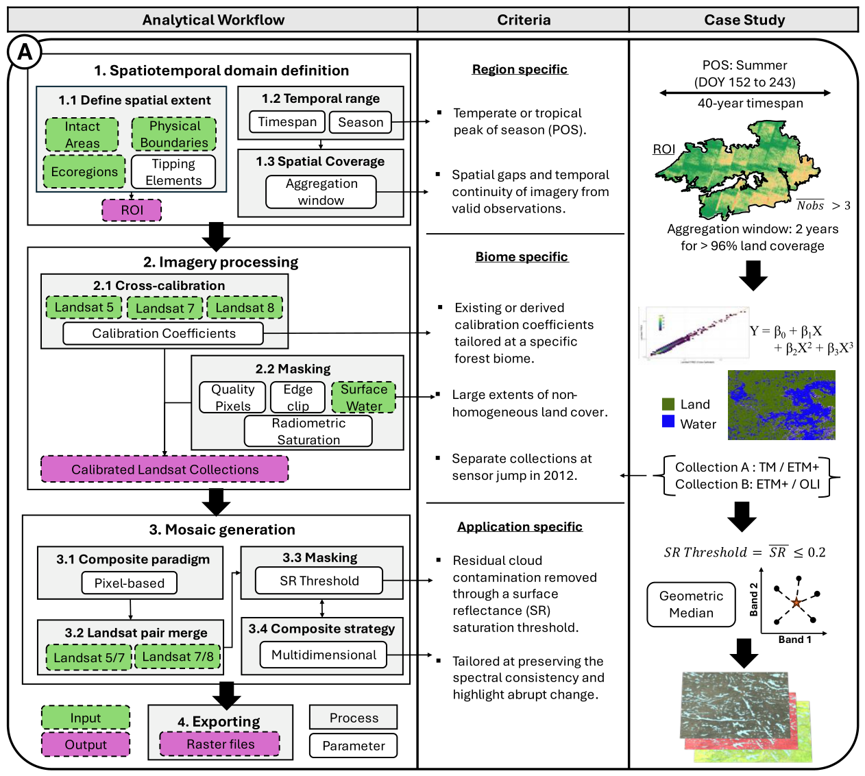
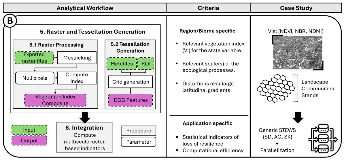
Figure 2.
Methodological scheme for the generation of long-term high-quality Landsat composites and the computation of statistical indicators of resilience. The workflow and general criteria to address practical (i) and multispectral (ii) limitations (Panel A), along the multiscale grid approach to tackle the scale (iii) limitations (Panel B) are delineated. The corresponding examples from the case study are displayed as well. Nobs = number of observations per pixel. ROI = region of interest.
Figure 2.
Methodological scheme for the generation of long-term high-quality Landsat composites and the computation of statistical indicators of resilience. The workflow and general criteria to address practical (i) and multispectral (ii) limitations (Panel A), along the multiscale grid approach to tackle the scale (iii) limitations (Panel B) are delineated. The corresponding examples from the case study are displayed as well. Nobs = number of observations per pixel. ROI = region of interest.
2.1. Cross-Calibration for Long-Term Records
The Landsat collections available in Google Earth Engine (GEE) provide high-resolution satellite imagery with global coverage for over four decades since 1984 (Appendix S2). Nonetheless, systematic differences arising from slight variations in wavelengths between Landsat sensors can significantly impact multidecadal timeseries interpretation or subtle ecological change detection analyses (Hemati et al., 2021). The most recent version of Landsat products, Collection 2, has undergone important corrections by improving data interoperability between sensors (Crawford et al., 2023); however, differences from sensor specific wavelength ranges between the spectral bands remain. Consequently, sensor cross-calibration is still recommended to avoid the introduction of false trends (Berner et al., 2020; Chen et al., 2024; Trevisiol et al., 2024), from known minor reflectance discrepancies influencing multi-sensor data compatibility (Ju and Masek, 2016).
Calibration coefficients developed for past collections (Roy et al., 2016a), and linear regressions (Wu et al., 2022) were previously used to correct sensor bias and ensure radiometric consistency between sensor observations (Appendix S3Error! Reference source not found.). Recent collections, however, require up-to-date coefficients to ensure their ongoing compatibility. A recently developed algorithm to cross-calibrate spectral bands among Landsat sensors was implemented using the LandsatTS package in RStudio (Berner et al., 2023). Rather than normalising to a reference scene (Wang et al., 2025), it employs a machine learning approach that uses representative pixel samples across a region to standardise data to Landsat 7 ETM+, due to its temporal overlap with Landsat 5 TM and Landsat 8 OLI (Error! Reference source not found.). A polynomial regression model then computes calibration coefficients derived from pixels within the study region, suggested to be good practice for change detection analysis (Richardson et al., 2025). The coefficients were applied to their corresponding Landsat collections in GEE, adjusting each surface reflectance (SR) band values to the fitted polynomial relationship (Error! Reference source not found. and Error! Reference source not found.). This bandpass adjustment offers a Landsat dataset specifically calibrated for an ecoregion or biome, minimizing the limitations of merging records from various sensors. Likewise, VIs derived from calibrated SR bands can be used as spatially explicit proxies of vegetation condition, including ecological responses to environmental change (Pettorelli et al., 2005), land monitoring and mapping (Wulder et al., 2008) at broad spatial extents.
2.2. Compositing for Resilience Indicators
The framework for generating high-quality, cloud-free images of the landscape was adapted from Li et al., (2019), implementing a pixel-based composite paradigm that selects the most representative reflectance value across all available Landsat scenes over the compositing period. First, imagery with less than 70% cloud cover was retained to avoid geometric correction errors, when reference points used to align each image to the ground are obscured by clouds (Goward et al., 2022). Second, the Quality Assessment (QA) bands were used to mask unreliable pixels, including those saturated, filled, or affected by clouds, cloud shadows, snow or ice features. Persistent residual contamination where QA masking omitted cloud or haze pixels (Hughes and Kennedy, 2019) was removed using post-compositing thresholds for unusually bright pixels (Sun et al., 2016). Water pixels were also masked, using the JRC global surface water dataset (Pekel et al., 2016), since they alter spatial metrics by decreasing spatial autocorrelation of surrounding land pixels due to their contrasting spatial patterns (Griffith and Chun, 2016). Additionally, edge cropping was applied to remove artifacts within ~0.5 km margins of the Landsat scenes, mostly associated with TM and ETM+ sensors (Robinson et al., 2017).
The preservation of spectral covariance structure across bands is also essential for the reliable computation of indicators (Smith et al., 2023; Smith and Boers, 2023). While algorithm performance is context-dependent with no one-size-fits-all method (Qiu et al., 2023), the geometric median (GeoMedian) based compositing has been suggested to provide a robust representation of a given period, even when the number of clear observations over large spatial extents is low (Roberts et al., 2017). In fact, annual high-quality GeoMedian composites, such as the GeoMAD Digital Earth Africa and Digital Earth Australia products, are highly suitable for spatial EWS analysis (Roberts et al., 2018) and classification (Wellington and Renzullo, 2021). Unlike pixel-selection compositing methods which select a single real observation such as the medoid and best available pixel (BAP), the GeoMedian computes a representative synthetic pixel by considering each clear observation as a point in a multi-band reflectance space and selecting the multivariate centre that minimises the summed Euclidean distance to all observations (Flood, 2013; Roberts et al., 2017). This avoids the mathematical biases introduced by temporal aggregation (Liu et al., 2026), reduces spatial noise, improves radiometric consistency, and better preserves the spectral relationships among bands (Francini et al., 2023).
By contrast, selecting single observations produces spatially discontinuous outputs (Meng et al., 2023), especially when neighbouring pixels are drawn from different acquisition dates (Roberts et al., 2017). For example, the maximum value composite (MVC) of the normalised difference vegetation index (NDVI) is a widely used approach for capturing peak vegetation growth, as it selects the greenest pixel values (Holben, 1986), which better discriminates against snow and cloud cover than mean and median compositing (Qiu et al., 2023). However, residual cloud shadows can mistakenly generate anomalously high NDVI values (Sousa et al., 2003). This is further compounded by an inherent bias towards phenological extremes, producing less radiometrically consistent image mosaics (Van doninck and Tuomisto, 2017) and reducing the contrast between vegetation types such as trees and grasslands (Flood, 2013). Moreover, MVC is sensitive to directional reflectance effects which, even though smaller for Landsat compared to wide-swath sensors (e.g. MODIS), remain non-negligible at high latitudes (Roy et al., 2016b). These effects are mitigated by the GeoMedian (Roberts et al., 2017), providing a particularly well-suited approach for peak of season (POS) compositing for temperate and tropical forest landscapes.
In addition, since conventional temporal EWS indicators are sensitive to residual non-stationarity and noise structure, rather than to the absolute magnitude of the underlying signal, compositing approaches that retain greater artifact-driven variability (e.g. MVC), risk generating spurious trends independent of genuine loss of resilience (Boettner and Boers, 2022; Dakos et al., 2012a). This is expected to be more pronounced for spatial EWS, rendering artifact removal critical for the utilisation of VIs for monitoring resilience (Zeng et al., 2022). Conversely, limitations of temporal aggregation are avoided by spatial EWS (Kéfi et al., 2014; MacLaren et al., 2025), because they do not necessarily require high-frequency timeseries to detect CSD trends (Butitta et al., 2017). The aggregation window length is ecosystem-specific and defined as the POS, when the dominant vegetation reaches peak phenology (Jeganathan et al., 2014). This is the summer months in boreal and temperate forests (Jarvis and Leverenz, 1983; Myneni et al., 1998) and the period of maximum solar radiation in tropical forests (Huete et al., 2006; Myneni et al., 2007).
2.3. Hexagonal Grids for Multiscale Indicators
To ensure that indicators computed from biophysical proxies are comparable across regions and scales of analysis, a reproducible approach for partitioning the landscape into consistent spatial units is necessary to reduce their sensitivity to arbitrary zoning and resolution choices (Jelinski and Wu, 1996). Squared grids are frequently used because of their congruency and alignment for grid partitioning (Birch et al., 2007). However, they become significantly affected by distortions when assessing large extents of the Earth (Sahr et al., 2003), particularly at higher latitudes (Fletcher, 2023). Avoiding this is crucial when assessing STEWS over extensive areas across different biomes.
Unlike conventional squared grids (Feng et al., 2024), Hexagonal Discrete Global Grids (HDGGs) result in compact equal-area tessellations that reduce directionality bias, provide uniform adjacency, and preserve equal area on the sphere (Kimerling et al., 1999a; Uher et al., 2019). Their applications have proven suitable for constructing globally consistent spatial units that minimize geometric and statistical artifacts (Sahr et al., 2003). Existing HDGG configurations provide balanced compromises between equal-area features, near-isotropic cell geometry, and a hierarchical index system (Kimerling et al., 1999b; Kmoch et al., 2025), which is well suited for environmental analyses at various scales (Birch et al., 2007). These features are advantageous when dealing with substantial geospatial datasets through cloud computing and parallel processing, supporting statistically robust spatial aggregation and map-based operations (Li and Stefanakis, 2020), while improving efficiency of STEWS computation (Appendix S3).
Multiple HDGGs were generated using the DGGRID open-source Python implementation (Sahr, 2025). Compared to other open-source tools (Kmoch et al., 2022a, 2022b), DGGRID provided a reproducible workflow which facilitated the construction of tessellations that can be seamlessly incorporated into standard GIS software as vector layers (Barnes, 2018). We propose HDGGs as a multiscale approach for unbiased cross-biome comparisons, expected to help in the identification of appropriate observation scales for system-specific ecological process, indicators or proxies.
2.4. The Boreal Forest: A Case Study in Eastern Canada
Boreal forests are currently experiencing some of the fastest and most significant warming on the planet (IPCC, 2022), and have been reported as a tipping element of the Earth’s biosphere (Armstrong McKay et al., 2022; Lenton et al., 2008). Despite diverging findings on boreal forest resilience, with reported declines (Smith et al., 2022) and increases (Forzieri et al., 2022; Southworth et al., 2023), evidence of an undergoing southern dieback and a northern expansion (Rotbarth et al., 2023) suggests it is potentially transitioning from the current bimodal distribution of tree cover, consisting mostly of either dense forests or sparse woodlands, towards a unimodal semi-open state with intermediate tree cover (Rotbarth et al., 2025). The observed trends of greening and densification in the northern interior forests (Berner and Goetz, 2022; Sulla-Menashe et al., 2018; Zhang et al., 2024) are consistent with the patterns of boreal forest change.
Although large disturbance footprints are captured by coarser spatial resolution imagery, small disturbances often remain under-detected (Bucha and Stibig, 2008; Jin and Sader, 2005; Potapov et al., 2008). Considering the broad spatiotemporal scales at which major disturbances typically trigger changes in the vegetation structure of boreal forests (Holling, 1992), finer-resolution datasets are required to resolve landscape changes (Wang and Friedl, 2019). The relatively high resolution of Landsat captures the stand and patch scales at which boreal disturbance and recovery processes occur (Frazier et al., 2015; White, 2024; White et al., 2017), closer to the key ecological scales that better capture boreal forest stability and change (Berner et al., 2020). In fact, Landsat has been able to characterize forest dynamics related to disturbances and climate-induced growth (Wang et al., 2020), including insect defoliation (Rahimzadeh-Bajgiran et al., 2018; Townsend et al., 2012), wildfires and timber harvest (Schroeder et al., 2011). These inherently spatial phenomena (Seidl et al., 2023) are often missed or aggregated away in coarse resolution sensors, such as MODIS or AVHRR, and resilience monitoring products (Zhang and Liu, 2024). In addition, Landsat’s native compatibility with the National Forest Inventory (NFI) and National Terrestrial Ecosystem Monitoring System (NTEMS) datasets, developed to annually quantify and characterise forest change (Hermosilla et al., 2016; Wulder et al., 2012), provides a further advantage of using Landsat to quantify forest resilience. The HDGG resolution levels considered in the tessellation analysis were then ecologically linked to the hierarchical structure of the boreal forest (Holling, 1992), comprising the stand, community and landscape scales across five different configurations (Error! Reference source not found.8).
To facilitate robust testing of our framework, we chose a large, undisturbed region of the boreal forest in northern Quebec as our case study (Error! Reference source not found.), based on the intact forest landscapes (IFL) dataset (Potapov et al., 2017). This selection minimises the influence of anthropogenic disturbances, allowing us to focus on natural disturbances and thereby simplifying the evaluation of our framework. The case study area is sufficiently large to accommodate the broad range of HDGG extents and configurations. Covering 325,514.11 km2, approximately 2.5 times the size of England, it enables the demonstration of the utility of our proposed scale-aware study design (Chave, 2013). It is worth noting that while IFL areas have no evidence of anthropogenic disturbances, natural disturbances such as wildfires still occur within them. Nevertheless, compared to similar areas in western Canada, the Eastern Canadian shield taiga remained relatively undisturbed until the wildfires of unprecedented scale and severity in 2023 (Byrne et al., 2024). Following the spatial extent delimitation, steps 1 to 3 of the framework (Error! Reference source not found., Panel A) were implemented.
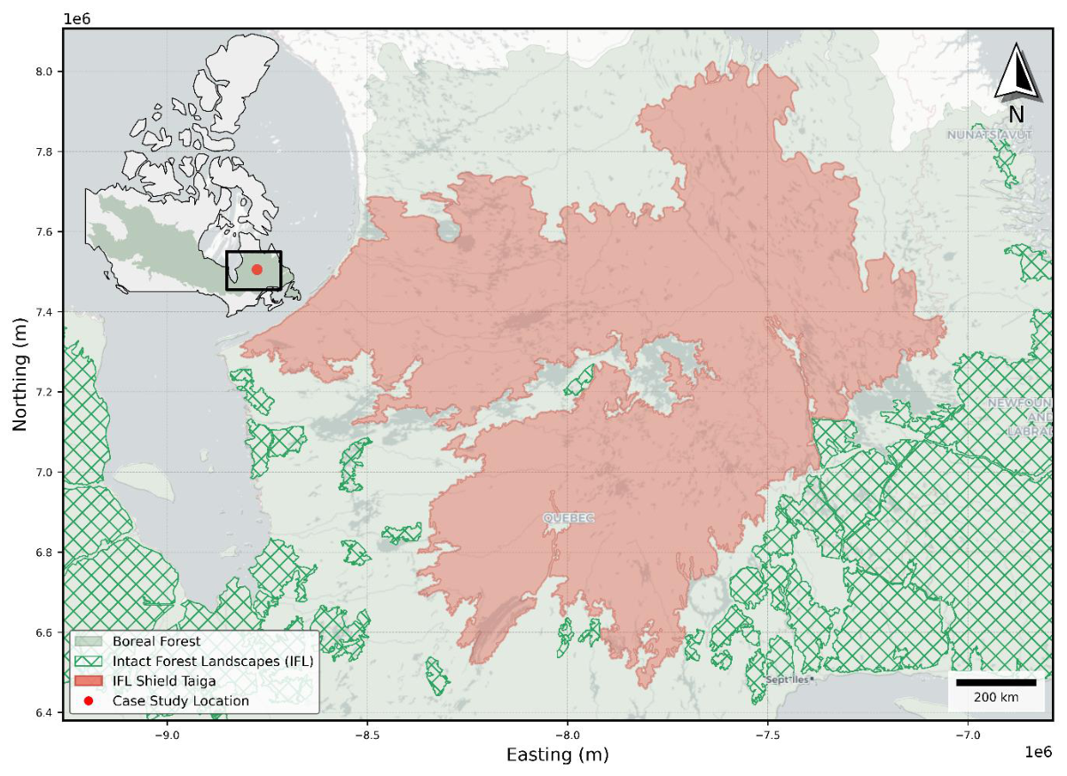
Figure 3.
Spatial extent of the region of interest (ROI in red) corresponding to an undisturbed boreal forest area in Quebec, Eastern Canada.
Figure 3.
Spatial extent of the region of interest (ROI in red) corresponding to an undisturbed boreal forest area in Quebec, Eastern Canada.
The quality of the composites was evaluated for data gaps, noise and radiometric consistency according to the criteria for pixel-based Landsat composite assessment delineated by Francini et al., (2023). The revised composites were then exported and mosaicked in RStudio to build VIs raster stacks from which indicators (i.e. spatial variance, autocorrelation and skewness) at five different HDGGs scales were computed, following steps 5 and 6 (Error! Reference source not found., Panel B). The processing parameters chosen specifically for the case study ecoregion are depicted in Error! Reference source not found..
3. Results
3.1. Reducing Multispectral Limitations
Spatially and radiometrically consistent cloud-free composites were generated for all SR bands. For the chosen region in Quebec, a two-year aggregation window was determined to be adequate to achieve near-complete land coverage (≥ 96%) for all composites, significantly reducing the spatial gaps (Error! Reference source not found.). This was determined based on the total number of observations available for annual composites being notably less when compared to biennial composites, especially for the periods when Landsat 5 provided the only available imagery (Error! Reference source not found., Panel A). The incorporation of Landsat 7 ETM+ was also required to achieve constant total (Error! Reference source not found., Panel B) and per month (Error! Reference source not found.Error! Reference source not found.) numbers of observations between composites, as the additional observations it provided significantly reduced the spatial gaps across the composites.
The resulting biennial composites were consequently distributed into fourteen composites between 1984 and 2011 and six composites between 2013 and 2024, constituting a dataset with a total of 20 composites. It is worth noting that a one-year gap corresponding to the summer of 2012 remained, since there is no dataset overlap between the Landsat 5 TM and Landsat 8 OLI collections, negatively impacting the number of observations available. Nonetheless, the incorporation of the available imagery from 2012 was tested to determine whether this had any significant impact on the composites and trends observed, with no significant change on the overall trend observed (Error! Reference source not found.). Incorporating the Landsat 7 ETM+ data to specifically account for 2012 in the timeseries was then deemed unnecessary, as the available observations for the selected years were already satisfactory and its inclusion would result in inconsistent aggregation windows.
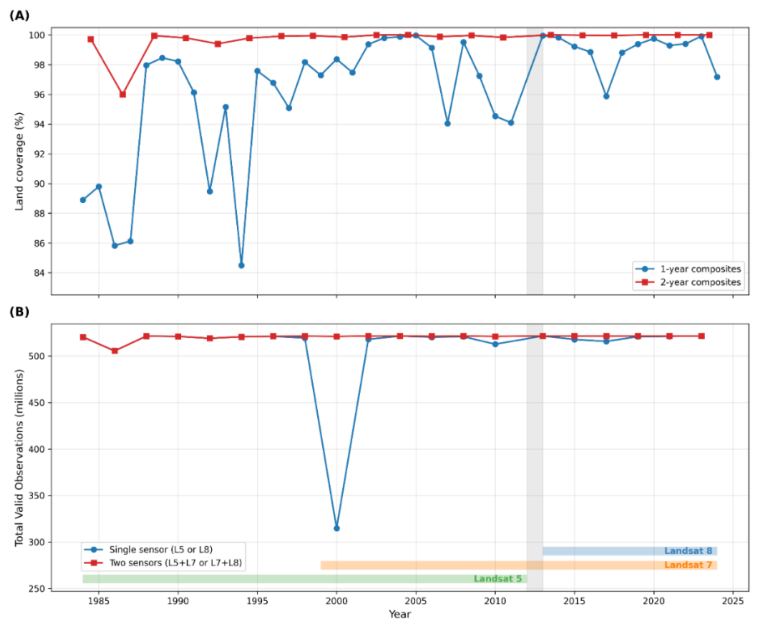
Figure 4.
Valid number of observations available for (A) land coverage between one- and two-year composites, and (B) for the total area when applying a one- and two-year aggregation window. The temporal coverage of each Landsat sensor is displayed at the bottom of panel (B). The shaded grey area indicates the gap year (2012).
Figure 4.
Valid number of observations available for (A) land coverage between one- and two-year composites, and (B) for the total area when applying a one- and two-year aggregation window. The temporal coverage of each Landsat sensor is displayed at the bottom of panel (B). The shaded grey area indicates the gap year (2012).
Both the MVC and GeoMedian approaches were compared to provide insights into the suitability of incorporating the latter in the proposed scheme. The GeoMedian was particularly effective at suppressing artifacts commonly found in optical satellite imagery (Figure 1). It successfully reduced the presence of ETM+ stripes (SCL-off), along with eliminating residual haze and shadow noise. Residual cloud contamination was observed for the GeoMedian composites in cases with fewer available observations (Figure 1, Panel E). These were removed using a saturation threshold derived from the mean reflectance value across all bands, selected empirically as 0.2 from visual inspection for this study area. Altogether, the spatial and radiometric consistency of the composites was improved, supporting the reliable computation of STEWS from Landsat imagery and the use of the GeoMedian approach for doing so.
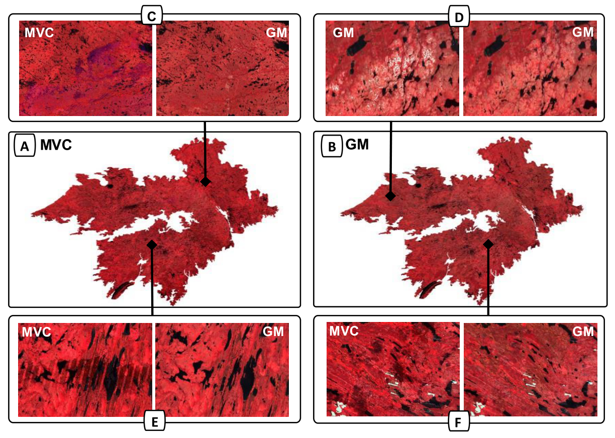
Figure 1.
Landsat composite comparison between the (A) MVC NDVI and (B) GeoMedian (GM) approaches, displaying improved artifact removal for spatial consistency for the latter. Samples from the biennial composite show differences in atmospheric haze (C), residual clouds (C), SCL-off stripes (E) and residual shadows (F). Images in false colour infrared (SR bands 5/4/3) band combination without water mask to highlight vegetation cover (in red hues), contrasting water bodies (dark blue or black).
Figure 1.
Landsat composite comparison between the (A) MVC NDVI and (B) GeoMedian (GM) approaches, displaying improved artifact removal for spatial consistency for the latter. Samples from the biennial composite show differences in atmospheric haze (C), residual clouds (C), SCL-off stripes (E) and residual shadows (F). Images in false colour infrared (SR bands 5/4/3) band combination without water mask to highlight vegetation cover (in red hues), contrasting water bodies (dark blue or black).
3.2. Merging the Landsat Collections
Region-specific calibration coefficients were derived from representative pixel samples across the province of Quebec (Error! Reference source not found.A). The obtained coefficients were similar to the ones provided by Berner et al. (2023) from a high-latitude dataset of randomly sampled terrestrial locations within the Arctic tundra and boreal forest biomes globally (Error! Reference source not found.). Small variations in coefficient values arise partly because the collections of pixel samples extracted from the imagery differ between calibrations. In addition, the calibration functions have some degree of random sub-setting of those samples, which causes the model coefficients to vary even if run multiple times on the same dataset. This resulted in slightly different NDVI timeseries (Table S7), but with the overall trends remaining quite consistent across networks of sites for both the MVC (Error! Reference source not found.) and the GM (Error! Reference source not found.). As expected for coefficients tailored to the same biome, the results were similar when applying them to the Landsat imagery as both sample sizes were large.
Temporal trends in mean NDVI from 1984 to 2024 evidenced the greening of the boreal forest biome of Quebec (Figure 6). The NDVI was taken as an exemplar to evaluate the composite timeseries as it is primarily associated with the reported greening trends. An analysis of the greening trend in NDVI illustrates the value of the compositing and calibration pipeline we propose, as it adjusts the magnitude and rate of the overall NDVI trend. Even though an increasing trend in NDVI was consistently observed, the rate of change varies significantly. Uncalibrated versions of the Landsat dataset were particularly different from calibrated ones, inflating the trends (0.0035 ± 0.0007 NDVI/yr), compared with calibrated datasets (0.0017 ± 0.0008 NDVI/yr). This reflects the systematic offset introduced by uncalibrated sensor transitions, which is observed in the abrupt discontinuity of the NDVI increase when Landsat sensors shift (Figure 6), particularly after 2012, when Landsat 5 imagery was no longer available, and Landsat 8 was introduced. The influence of sensor-shift induced leaps in the timeseries was further reduced by the incorporation of Landsat 7, although trends remained comparable within both the calibrated and uncalibrated versions.
Similarly, the compositing strategy impacted the magnitude of the trend, where MVC trends were steeper compared to the GeoMedian calibrated trends, inflated by 40.2% for the calibrated MVC (Figure S6), and up to 130.7% for the uncalibrated MVC. Cross-calibrating was clearly beneficial to reduce the influence of sensor shift leaps on the timeseries. This highlights the importance of carefully distinguishing an increase in NDVI as evidence of canopy densification, a shift toward broadleaf dominance, or recovery from disturbance. The GeoMedian compositing strategy, along with the regional cross-calibration coefficients, provided a higher spatial and temporal consistency across the composites for a more reliable computation of STEWS from Landsat imagery.
3.3. Beyond Pixels with Multiscale Grids
The HDGGs enabled the re-sampling of the Landsat data into ecologically meaningful units. This allowed for STEWS to be calculated at multiple scales of observation. The effect of scale of observation and resolution could then be assessed using varying grid configurations and resolutions. Integrating a multiscale grid system to analyse biomes at relevant, ecologically grounded scales is crucial for ecological applications of EWS. While processing higher resolution imagery is computationally expensive, our HDGG approach also addresses this via parallelisation. It greatly improved the computation times of indicators from raster data (Error! Reference source not found.Error! Reference source not found.), reducing overall processing times by 69.6% compared to sequential attempts.
4. Discussion
Our workflow provided consistent high-quality Landsat composites for a large region of the boreal forest in eastern Canada utilising the full Landsat Collection-2 archive. It therefore represents an important advance for existing studies that use Landsat-derived EWS to assess forest resilience. These have generally covered shorter time windows at local or regional scales (Liu et al., 2019; Vargas et al., 2019; Wu et al., 2022). Hui Wang et al. (2025) combined all three sensors (TM, ETM+ and OLI) over a ~16-year window to evaluate local vegetation resilience. Rogers et al. (2018) detected EWS of tree mortality across boreal North America over a ~28-year window but including two sensors (TM and ETM+). The employed Landsat-derived NDVI timeseries addressed multi-sensor differences with a scaling factor (Ju and Masek, 2016), primarily calibrating at the NDVI-level. However, index-level cross-calibration does not eliminate per-band reflectance discontinuities, which are known to introduce artificial long-term trends in combined NDVI records (Sulla-Menashe et al., 2016), to which statistical indicators are particularly sensitive (Dakos et al., 2012b; Lenton et al., 2012). Our study clearly show that the region-specific calibration coefficients allowed for a consistent multi-sensor Landsat record suitable for reliable resilience analysis. Global scale monitoring of the boreal forest could rely on existing, already-developed biome-specific coefficients. Therefore, we recommend deriving broader biome-level calibration coefficients for further terrestrial ecosystems (e.g. rainforests, temperate forests and drylands) and, if necessary, compare with regionally specific coefficients.
Our study used a relatively long aggregation window of two years, as for forest ecosystems, longer aggregation windows may be acceptable due to their higher stability and slower vegetation dynamics compared to grasslands and drylands (Han et al., 2025). However, the length of the aggregation window can be dynamically adjusted within our framework based on the local density of cloud-free observations, or the characteristic ecological recovery timescale of the specific biome under study. As such, shorter aggregation windows are possible for less extensive and/or less cloudy regions, allowing for annual composites to increase temporal resolution.
Through our case study it was also confirmed that without a built-in bias toward greenness, the GeoMedian obtains a physically representative state over the entire compositing period, capturing abrupt changes between compositing periods. While it smooths out rapid within-period events (Roberts et al., 2017), the GeoMedian excels at detecting cross-period long-term changes rather than transient fluctuations (Gupta et al., 2024), making it ideally suited for spatial EWS. By contrast, the MVC algorithm will actively avoid these observations since disturbances usually represent a state of low productivity (Flood, 2013). With at least one pixel observation from a pre-disturbance and/or a recovered post-disturbance state, disturbances within the aggregation window are effectively removed from the MVC composite. The associated timeseries would then only reflect the most productive state of the landscape rather than its actual average condition.
Furthermore, our framework can be applied for any VI. This is important, as the choice of VIs should be tailored to the target ecosystem or biome, as different indices vary in their sensitivity and applicability across vegetation types (Lenton et al., 2022; Zeng et al., 2022). We therefore recommend employing multiple VIs when drawing ecological interpretations to improve robustness and reduce the risk of biome-specific bias. For instance, in the boreal forest, an increase in broadleaf species relative to conifer-dominated stands following disturbance is expected to be reflected in the increase of vegetation productivity indices, such as the Enhanced Vegetation Index (EVI) and NDVI (Fiore et al., 2020; White et al., 2023). By contrast, other VIs are spatially correlated to natural disturbances such as wildfires and insect outbreaks (Mackey et al., 2024). The Normalized Burn Ratio (NBR), for example, is more sensitive to structural recovery of the canopy (Pickell et al., 2016). Similarly, the Shortwave Infrared Water Stress Index (SIWSI) captures water-stressed canopies (Shestakova et al., 2024), whereas the Normalized Difference Moisture Index (NDMI) decreases under drought stress and pre-fire fuel availability (Sivrikaya et al., 2024), distinguishing canopy water content from structural or compositional change. Indices derived from the near-infrared (NIR) and shortwave infrared (SWIR) bands (i.e. NBR, NDMI and SIWSI) tend to be more strongly correlated with changes in above-ground biomass than greenness-based indices are (Meimand et al., 2026). Therefore, to better identify processes driving a given trend (e.g. stand succession, biome-margin shift, shrubification, tree mortality), complementary indices serve specific disambiguation roles. Our framework is also flexible enough to enable future work which could incorporate biophysical or structural variables such as fraction of photosynthetically active radiation (fAPAR) or leaf area index (LAI), which are less confounded by ground surface reflectance, atmospheric conditions, and sensor characteristics (Myneni and Williams, 1994).
Future work should consider integrating Landsat 9, given the mission continuity it provides (Masek et al., 2020) and its robust instrument similarity to Landsat 8 (Gross et al., 2022), although sensor-specific cross-calibration or transformation coefficients (Zhang et al., 2025) remain necessary to ensure inter-sensor consistency. On the other hand, geospatial foundation models that generate satellite embeddings from multi-sensor imagery, such as AlphaEarth Foundations (Brown et al., 2025) and TESSERA (Feng et al., 2026), represent a different paradigm in which sensor harmonization is learned as part of model training rather than applied as a separate calibration step. Beyond this conceptual difference, both products are currently restricted to the Sentinel-era archive (2017 onwards) and cannot yet support the multi-decadal analysis required to detect ecological tipping points. Their ecological interpretability would also likely prove more challenging compared to VIs based on physical reflectance properties. AlphaEarth native availability in GEE could nonetheless make it useful as a complementary validation layer for recent periods, since it could integrate easily with existing repositories.
Consistent, cross-calibrated long-term archives such as Landsat remain essential for monitoring forest resilience at large scales, especially as a global decline in vegetation resilience since the early 2000s has been reported (Forzieri et al., 2022; Rocha, 2022; Seddon et al., 2016; Smith et al., 2022; Zhang et al., 2024). Tropical rainforests have shown slower recovery rates under drier conditions associated with mean annual precipitation declines (Verbesselt et al., 2016). This is particularly evident in the Amazon rainforest where loss of resilience driven by deforestation and climate change is increasing the likelihood of rainforest dieback (Boulton et al., 2022; Van Passel et al., 2024; Wang et al., 2024). Similarly, significant declines in the resilience of the northwestern American boreal forests have been detected in regions affected by forest losses and wildfires along the southern margins of warm, dry and densely vegetated areas (Rotbarth et al., 2025, 2023; Zhang et al., 2024). In contrast, other studies report opposite patterns, with increasing resilience in boreal forests accompanied by declining resilience in tropical rainforests (Forzieri et al., 2022; Southworth et al., 2023) or, conversely, increasing resilience in the tropics coupled with declining resilience at higher latitudes (Smith et al., 2022). While forest vegetation responses are highly variable when measured by season, biome and land use (Saatchi et al., 2021; Southworth et al., 2023), these divergent findings may be partly attributable to variable practices for measuring resilience in forest systems, along with the spatiotemporal scales at which forests are being monitored. Resolving these discrepancies requires consistent methodological frameworks, such as the one developed here for Landsat data, to support the application of EWS across forest ecoregions that reliably characterize the changing resilience of Earth tipping elements.
5. Conclusion
The utilisation of satellite EO for measuring ecosystem resilience through statistical indicators has been widely explored across terrestrial biomes. Long-term remote sensing data should be carefully treated when applied to measure loss of ecosystem resilience because current EO limitations for detecting EWS need to be considered. Reliable indicators of resilience often require (i) long-term timeseries, (ii) consistent spatial data and (iii) scale-aware approaches. We have presented a methodological framework that minimizes these limitations by leveraging the full length of the higher-resolution Landsat archive for resilience assessments. While no single compositing or calibration approach is unambiguously optimal for all applications, we outline the approach we consider best suited for STEWS computation, on the basis that it minimises the artifact-driven non-stationarity to which indicators are particularly sensitive. The regionally cross-calibrated GeoMedian composites provided a consistent multi-sensor Landsat record suitable for a more reliable forest resilience assessment, though further testing would be needed for non-boreal biomes. Critically, our framework’s multiscale HDGG approach provides a highly efficient way to process EO data through parallel processing that is scale-comparable because of the indexing system it offers, and which can be easily integrated with additional geospatial datasets, thereby, providing a consistent method for quantifying STEWS in any terrestrial ecosystem. In combination, application of our framework could shed light on the discrepancies among the trends observed from different indicators and approaches applied to ecosystems worldwide. This is central to understanding how forest biomes are changing, and to assessing whether they are approaching critical transitions.
Supplementary Materials
The following supporting information can be downloaded at the website of this paper posted on Preprints.org.
Author Contributions
Cesar Murad: conceptualisation, writing - original draft, investigation, visualisation, methodology, validation, formal analysis, data curation, writing - review & editing. Felix Eigenbrod: writing – review & editing, methodology, supervision. Jadu Dash: writing – review & editing, methodology, supervision. John Dearing: writing – review & editing, supervision. Neil Brummitt: writing – review & editing, supervision.
Acknowledgments
This study was supported by the UKRI NERC Interdisciplinary Southampton Partnership for Investigators Researching the Environment (INSPIRE) Doctoral Training Partnership (NE/S007210/1). For the purpose of open access, the author has applied a Creative Commons attribution license (CC BY) to any Author Accepted Manuscript version arising from this submission.
Conflicts of Interest
The authors declare no conflicts of interest.
Declaration on the Use of AI
Generative artificial intelligence (AI) tools use has been restricted to debugging and occasional code assistance. All conceptual development, analysis, and written content remain our own, and no AI-generated material is included in this submission.
Data Accessibility
The JavaScript and RStudio scripts for the case study analysis are available on GitHub https://github.com/camuradr/LandsatCompositesGEE and can be modified with custom input parameters.
References
- Alibakhshi, S.; Groen, T.A.; Rautiainen, M.; Naimi, B. Remotely-Sensed Early Warning Signals of a Critical Transition in a Wetland Ecosystem. Remote Sens. 2017, 9. [Google Scholar] [CrossRef]
- Armstrong McKay, D.I.; Staal, A.; Abrams, J.F.; Winkelmann, R.; Sakschewski, B.; Loriani, S.; Fetzer, I.; Cornell, S.E.; Rockström, J.; Lenton, T.M. Exceeding 1.5°C global warming could trigger multiple climate tipping points. Science 2022, 377, eabn7950. [Google Scholar] [CrossRef]
- Banskota, A.; Kayastha, N.; Falkowski, M.J.; Wulder, M.A.; Froese, R.E.; White, J.C. Forest Monitoring Using Landsat Time Series Data: A Review. Can. J. Remote Sens. 2014, 40, 362–384. [Google Scholar] [CrossRef]
- Barnes, R. r-barnes/dggridR: v2.0.3. 2018. [Google Scholar] [CrossRef]
- Bastiaansen, R.; Doelman, A.; Eppinga, M.B.; Rietkerk, M. The effect of climate change on the resilience of ecosystems with adaptive spatial pattern formation. Ecol. Lett. 2020, 23, 414–429. [Google Scholar] [CrossRef]
- Bathiany, S.; Bastiaansen, R.; Bastos, A.; Blaschke, L.; Lever, J.; Loriani, S.; De Keersmaecker, W.; Dorigo, W.; Milenković, M.; Senf, C.; Smith, T.; Verbesselt, J.; Boers, N. Ecosystem Resilience Monitoring and Early Warning Using Earth Observation Data: Challenges and Outlook. Surv. Geophys. 2025, 46, 265–301. [Google Scholar] [CrossRef]
- Berner, L.T.; Assmann, J.J.; Normand, S.; Goetz, S.J. ‘LandsatTS’: an R package to facilitate retrieval, cleaning, cross-calibration, and phenological modeling of Landsat time series data. Ecography 2023, e06768. [Google Scholar] [CrossRef]
- Berner, L.T.; Goetz, S.J. Satellite observations document trends consistent with a boreal forest biome shift. Glob. Change Biol. 2022, 28, 3275–3292. [Google Scholar] [CrossRef]
- Berner, L.T.; Massey, R.; Jantz, P.; Forbes, B.C.; Macias-Fauria, M.; Myers-Smith, I.; Kumpula, T.; Gauthier, G.; Andreu-Hayles, L.; Gaglioti, B.V.; Burns, P.; Zetterberg, P.; D’Arrigo, R.; Goetz, S.J. Summer warming explains widespread but not uniform greening in the Arctic tundra biome. Nat. Commun. 2020, 11, 4621. [Google Scholar] [CrossRef]
- Birch, C.P.D.; Oom, S.P.; Beecham, J.A. Rectangular and hexagonal grids used for observation, experiment and simulation in ecology. Ecol. Model. 2007, 206, 347–359. [Google Scholar] [CrossRef]
- Boettiger, C.; Ross, N.; Hastings, A. Early warning signals: the charted and uncharted territories. Theor. Ecol. 2013, 6, 255–264. [Google Scholar] [CrossRef]
- Boettner, C.; Boers, N. Critical slowing down in dynamical systems driven by nonstationary correlated noise. Phys. Rev. Res. 2022, 4, 013230. [Google Scholar] [CrossRef]
- Boulton, C.A.; Lenton, T.M.; Boers, N. Pronounced loss of Amazon rainforest resilience since the early 2000s. Nat. Clim. Change 2022, 12, 271–278. [Google Scholar] [CrossRef]
- Brown, C.F.; Kazmierski, M.R.; Pasquarella, V.J.; Rucklidge, W.J.; Samsikova, M.; Zhang, C.; Shelhamer, E.; Lahera, E.; Wiles, O.; Ilyushchenko, S.; Gorelick, N.; Zhang, L.L.; Alj, S.; Schechter, E.; Askay, S.; Guinan, O.; Moore, R.; Boukouvalas, A.; Kohli, P. AlphaEarth Foundations: An embedding field model for accurate and efficient global mapping from sparse label data. 2025. [Google Scholar] [CrossRef]
- Bucha, T.; Stibig, H.-J. Analysis of MODIS imagery for detection of clear cuts in the boreal forest in north-west Russia. Remote Sens. Environ. Earth Obs. Terr. Biodivers. Ecosyst. Spec. Issue 2008, 112, 2416–2429. [Google Scholar] [CrossRef]
- Butitta, V.L.; Carpenter, S.R.; Loken, L.C.; Pace, M.L.; Stanley, E.H. Spatial early warning signals in a lake manipulation. Ecosphere 2017, 8, e01941. [Google Scholar] [CrossRef]
- Byrne, B.; Liu, J.; Bowman, K.W.; Pascolini-Campbell, M.; Chatterjee, A.; Pandey, S.; Miyazaki, K.; van der Werf, G.R.; Wunch, D.; Wennberg, P.O.; Roehl, C.M.; Sinha, S. Carbon emissions from the 2023 Canadian wildfires. Nature 2024, 633, 835–839. [Google Scholar] [CrossRef]
- Cailleret, M.; Dakos, V.; Jansen, S.; Robert, E.M.R.; Aakala, T.; Amoroso, M.M.; Antos, J.A.; Bigler, C.; Bugmann, H.; Caccianaga, M.; Camarero, J.-J.; Cherubini, P.; Coyea, M.R.; Čufar, K.; Das, A.J.; Davi, H.; Gea-Izquierdo, G.; Gillner, S.; Haavik, L.J.; Hartmann, H.; Hereş, A.-M.; Hultine, K.R.; Janda, P.; Kane, J.M.; Kharuk, V.I.; Kitzberger, T.; Klein, T.; Levanic, T.; Linares, J.-C.; Lombardi, F.; Mäkinen, H.; Mészáros, I.; Metsaranta, J.M.; Oberhuber, W.; Papadopoulos, A.; Petritan, A.M.; Rohner, B.; Sangüesa-Barreda, G.; Smith, J.M.; Stan, A.B.; Stojanovic, D.B.; Suarez, M.-L.; Svoboda, M.; Trotsiuk, V.; Villalba, R.; Westwood, A.R.; Wyckoff, P.H.; Martínez-Vilalta, J. Early-Warning Signals of Individual Tree Mortality Based on Annual Radial Growth. Front. Plant Sci. 9. 2019. [Google Scholar] [CrossRef]
- Camarero, J.J.; Gazol, A.; Sangüesa-Barreda, G.; Oliva, J.; Vicente-Serrano, S.M. To die or not to die: early warnings of tree dieback in response to a severe drought. J. Ecol. 2015, 103, 44–57. [Google Scholar] [CrossRef]
- Carnicer, J.; Domingo-Marimon, C.; Ninyerola, M.; Camarero, J.J.; Bastos, A.; López-Parages, J.; Blanquer, L.; Rodríguez-Fonseca, B.; Lenton, T.M.; Dakos, V.; Ribas, M.; Gutiérrez, E.; Peñuelas, J.; Pons, X. Regime shifts of Mediterranean forest carbon uptake and reduced resilience driven by multidecadal ocean surface temperatures. Glob. Change Biol. 2019, 25, 2825–2840. [Google Scholar] [CrossRef]
- Chave, J. The problem of pattern and scale in ecology: what have we learned in 20 years? Ecol. Lett. 2013, 16, 4–16. [Google Scholar] [CrossRef]
- Chen, S.; Wang, J.; Liu, Q.; Liang, X.; Liu, R.; Qin, P.; Yuan, J.; Wei, J.; Yuan, S.; Huang, H.; Gong, P. Global 30 m seamless data cube (2000–2022) of land surface reflectance generated from Landsat 5, 7, 8, and 9 and MODIS Terra constellations. Earth Syst. Sci. Data 2024, 16, 5449–5475. [Google Scholar] [CrossRef]
- Claverie, M.; Ju, J.; Masek, J.G.; Dungan, J.L.; Vermote, E.F.; Roger, J.-C.; Skakun, S.V.; Justice, C. The Harmonized Landsat and Sentinel-2 surface reflectance data set. Remote Sens. Environ. 2018, 219, 145–161. [Google Scholar] [CrossRef]
- Cohen, W.B.; Goward, S.N. Landsat’s Role in Ecological Applications of Remote Sensing. BioScience 2004, 54, 535–545. [Google Scholar]
- Colangelo, M.; Camarero, J.J.; Borghetti, M.; Gazol, A.; Gentilesca, T.; Ripullone, F. Size Matters a Lot: Drought-Affected Italian Oaks Are Smaller and Show Lower Growth Prior to Tree Death. Front. Plant Sci. 2017, 8. [Google Scholar] [CrossRef]
- Cracknell, A.P. The Advanced Very High Resolution Radiometer AVHRR; CRC Press: London, 2024. [Google Scholar] [CrossRef]
- Crawford, C.J.; Roy, D.P.; Arab, S.; Barnes, C.; Vermote, E.; Hulley, G.; Gerace, A.; Choate, M.; Engebretson, C.; Micijevic, E.; Schmidt, G.; Anderson, C.; Anderson, M.; Bouchard, M.; Cook, B.; Dittmeier, R.; Howard, D.; Jenkerson, C.; Kim, M.; Kleyians, T.; Maiersperger, T.; Mueller, C.; Neigh, C.; Owen, L.; Page, B.; Pahlevan, N.; Rengarajan, R.; Roger, J.-C.; Sayler, K.; Scaramuzza, P.; Skakun, S.; Yan, L.; Zhang, H.K.; Zhu, Z.; Zahn, S. The 50-year Landsat collection 2 archive. Sci. Remote Sens. 2023, 8, 100103. [Google Scholar] [CrossRef]
- Dakos, V.; Boulton, C.A.; Buxton, J.E.; Abrams, J.F.; Arellano-Nava, B.; Armstrong McKay, D.I.; Bathiany, S.; Blaschke, L.; Boers, N.; Dylewsky, D.; López-Martínez, C.; Parry, I.; Ritchie, P.; van der Bolt, B.; van der Laan, L.; Weinans, E.; Kéfi, S. Tipping point detection and early warnings in climate, ecological, and human systems. Earth Syst. Dyn. 2024, 15, 1117–1135. [Google Scholar] [CrossRef]
- Dakos, V.; Carpenter, S.R.; Brock, W.A.; Ellison, A.M.; Guttal, V.; Ives, A.R.; Kéfi, S.; Livina, V.; Seekell, D.A.; van Nes, E.H.; Scheffer, M. Methods for Detecting Early Warnings of Critical Transitions in Time Series Illustrated Using Simulated Ecological Data. PLoS ONE 2012a, 7, e41010. [Google Scholar] [CrossRef]
- Dakos, V.; Scheffer, M.; van Nes, E.H.; Brovkin, V.; Petoukhov, V.; Held, H. Slowing down as an early warning signal for abrupt climate change. Proc. Natl. Acad. Sci. 2008, 105, 14308–14312. [Google Scholar] [CrossRef]
- Dakos, V.; van Nes, E.H.; D’Odorico, P.; Scheffer, M. Robustness of variance and autocorrelation as indicators of critical slowing down. Ecology 2012b, 93, 264–271. [Google Scholar] [CrossRef]
- Dwomoh, F.K.; Wimberly, M.C. Fire regimes and forest resilience: alternative vegetation states in the West African tropics. Landsc. Ecol. 2017, 32, 1849–1865. [Google Scholar] [CrossRef]
- Feng, X.; Rocha, T.; Thammavong, H.T.; Tulaiha, R.; Chen, X.; Xie, Y.; Park, D.S. GridDER: Grid Detection and Evaluation in R. Ecol. Inform. 2024, 79, 102391. [Google Scholar] [CrossRef]
- Feng, Z.; Atzberger, C.; Jaffer, S.; Knezevic, J.; Sormunen, S.; Young, R.; Lisaius, M.C.; Immitzer, M.; Jackson, T.; Ball, J.; Coomes, D.A.; Madhavapeddy, A.; Blake, A.; Keshav, S. TESSERA: Temporal Embeddings of Surface Spectra for Earth Representation and Analysis. 2026. [Google Scholar] [CrossRef]
- Fiore, N.M.; Goulden, M.L.; Czimczik, C.I.; Pedron, S.A.; Tayo, M.A. Do recent NDVI trends demonstrate boreal forest decline in Alaska? Environ. Res. Lett. 2020, 15, 095007. [Google Scholar] [CrossRef]
- Fletcher, S.J. Chapter 12 - Numerical Modeling on the Sphere. In Data Assimilation for the Geosciences (Second Edition); Fletcher, S.J., Ed.; Elsevier, 2023; pp. 485–555. [Google Scholar] [CrossRef]
- Flood, N. Seasonal Composite Landsat TM/ETM+ Images Using the Medoid (a Multi-Dimensional Median). Remote Sens. 2013, 5, 6481–6500. [Google Scholar] [CrossRef]
- Forzieri, G.; Dakos, V.; McDowell, N.G.; Ramdane, A.; Cescatti, A. Emerging signals of declining forest resilience under climate change. Nature 2022, 608, 534–539. [Google Scholar] [CrossRef]
- Francini, S.; Hermosilla, T.; Coops, N.C.; Wulder, M.A.; White, J.C.; Chirici, G. An assessment approach for pixel-based image composites. ISPRS J. Photogramm. Remote Sens. 2023, 202, 1–12. [Google Scholar] [CrossRef]
- Frazier, R.J.; Coops, N.C.; Wulder, M.A. Boreal Shield forest disturbance and recovery trends using Landsat time series. Remote Sens. Environ. 2015, 170, 317–327. [Google Scholar] [CrossRef]
- Goward, S.N.; Williams, D.L.; Arvidson, T.; Rocchio, L.E.; Irons, J.R.; Russell, C.A.; Johnston, S.S. Landsat’s Enduring Legacy: Pioneering Global Land Observations From Space. Photogramm. Eng. Remote Sens. 2022, 88. [Google Scholar] [CrossRef]
- Griffith, D.A.; Chun, Y. Spatial Autocorrelation and Uncertainty Associated with Remotely-Sensed Data. Remote Sens. 2016, 8, 535. [Google Scholar] [CrossRef]
- Gross, G.; Helder, D.; Begeman, C.; Leigh, L.; Kaewmanee, M.; Shah, R. Initial Cross-Calibration of Landsat 8 and Landsat 9 Using the Simultaneous Underfly Event. Remote Sens. 2022, 14, 2418. [Google Scholar] [CrossRef]
- Gupta, R.; Zuquim, G.; Tuomisto, H. Seamless Landsat-7 and Landsat-8 data composites covering all Amazonia. Data Brief. 2024, 57, 111034. [Google Scholar] [CrossRef]
- Han, Y.; Qu, Y.; Jiang, T.; Zhang, X.; Lyu, J.; Su, X. Ecosystems resilience assessment of forest and grassland subjected to ecological drought. Ecol. Indic. 2025, 173, 113437. [Google Scholar] [CrossRef]
- Hemati, M.; Hasanlou, M.; Mahdianpari, M.; Mohammadimanesh, F. A Systematic Review of Landsat Data for Change Detection Applications: 50 Years of Monitoring the Earth. Remote Sens. 2021, 13, 2869. [Google Scholar] [CrossRef]
- Hermosilla, T.; Wulder, Michael A.; White, Joanne C.; Coops, Nicholas C.; Hobart, Geordie W.; Campbell, L.B. Mass data processing of time series Landsat imagery: pixels to data products for forest monitoring. Int. J. Digit. Earth 2016, 9, 1035–1054. [Google Scholar] [CrossRef]
- Holben, B.N. Characteristics of maximum-value composite images from temporal AVHRR data. Int. J. Remote Sens. 1986, 7, 1417–1434. [Google Scholar] [CrossRef]
- Holling, C.S. The role of forest insects in structuring the boreal landscape. In A Systems Analysis of the Global Boreal Forest; Bonan, G.B., Shugart, H.H., Leemans, R., Eds.; Cambridge University Press: Cambridge, 1992; pp. 170–191. [Google Scholar] [CrossRef]
- Hu, Z.; Guo, Q.; Li, S.; Piao, S.; Knapp, A.K.; Ciais, P.; Li, X.; Yu, G. Shifts in the dynamics of productivity signal ecosystem state transitions at the biome-scale. Ecol. Lett. 2018, 21, 1457–1466. [Google Scholar] [CrossRef]
- Huete, A.R.; Didan, K.; Shimabukuro, Y.E.; Ratana, P.; Saleska, S.R.; Hutyra, L.R.; Yang, W.; Nemani, R.R.; Myneni, R. Amazon rainforests green-up with sunlight in dry season. Geophys. Res. Lett. 2006, 33. [Google Scholar] [CrossRef]
- Hughes, M.J.; Kennedy, R. High-Quality Cloud Masking of Landsat 8 Imagery Using Convolutional Neural Networks. Remote Sens. 2019, 11. [Google Scholar] [CrossRef]
- IPCC. IClimate Change and Land: IPCC Special Report on Climate Change, Desertification, Land Degradation, Sustainable Land Management, Food Security, and Greenhouse Gas Fluxes in Terrestrial Ecosystems, 1st ed.; Cambridge University Press, 2022. [Google Scholar] [CrossRef]
- Jarvis, P.G.; Leverenz, J.W. Productivity of Temperate, Deciduous and Evergreen Forests. In Physiological Plant Ecology IV: Ecosystem Processes: Mineral Cycling, Productivity and Man’s Influence; Lange, O.L., Nobel, P.S., Osmond, C.B., Ziegler, H., Eds.; Springer: Berlin, Heidelberg, 1983; pp. 233–280. [Google Scholar] [CrossRef]
- Jeganathan, C.; Dash, J.; Atkinson, P.M. Remotely sensed trends in the phenology of northern high latitude terrestrial vegetation, controlling for land cover change and vegetation type. Remote Sens. Environ. 2014, 143, 154–170. [Google Scholar] [CrossRef]
- Jelinski, D.E.; Wu, J. The modifiable areal unit problem and implications for landscape ecology. Landsc. Ecol. 1996, 11, 129–140. [Google Scholar] [CrossRef]
- Jiang, H.; Song, L.; Li, Y.; Ma, M.; Fan, L. Monitoring the Reduced Resilience of Forests in Southwest China Using Long-Term Remote Sensing Data. Remote Sens. 2021, 14. [Google Scholar] [CrossRef]
- Jin, S.; Sader, S.A. MODIS time-series imagery for forest disturbance detection and quantification of patch size effects. Remote Sens. Environ. 2005, 99, 462–470. [Google Scholar] [CrossRef]
- Ju, J.; Masek, J.G. The vegetation greenness trend in Canada and US Alaska from 1984–2012 Landsat data. Remote Sens. Environ. 2016, 176, 1–16. [Google Scholar] [CrossRef]
- Ju, J.; Zhou, Q.; Freitag, B.; Roy, D.P.; Zhang, H.K.; Sridhar, M.; Mandel, J.; Arab, S.; Schmidt, G.; Crawford, C.J.; Gascon, F.; Strobl, P.A.; Masek, J.G.; Neigh, C.S.R. The Harmonized Landsat and Sentinel-2 version 2.0 surface reflectance dataset. Remote Sens. Environ. 2025, 324, 114723. [Google Scholar] [CrossRef]
- Justice, C.O.; Townshend, J.R.G.; Vermote, E.F.; Masuoka, E.; Wolfe, R.E.; Saleous, N.; Roy, D.P.; Morisette, J.T. An overview of MODIS Land data processing and product status. Remote Sens. Environ. Moderate Resolut. Imaging Spectroradiometer (MODIS) A New Gener. Land Surf. Monit. 2002, 83, 3–15. [Google Scholar] [CrossRef]
- Kéfi, S.; Dakos, V.; Scheffer, M.; Van Nes, E.H.; Rietkerk, M. Early warning signals also precede non-catastrophic transitions. Oikos 2013, 122, 641–648. [Google Scholar] [CrossRef]
- Kéfi, S.; Guttal, V.; Brock, W.A.; Carpenter, S.R.; Ellison, A.M.; Livina, V.N.; Seekell, D.A.; Scheffer, M.; van Nes, E.H.; Dakos, V. Early Warning Signals of Ecological Transitions: Methods for Spatial Patterns. PLoS ONE 2014, 9, e92097. [Google Scholar] [CrossRef]
- Kennedy, R.E.; Yang, Z.; Cohen, W.B. Detecting trends in forest disturbance and recovery using yearly Landsat time series: 1. LandTrendr — Temporal segmentation algorithms. Remote Sens. Environ. 2010, 114, 2897–2910. [Google Scholar] [CrossRef]
- Kimerling, J.A.; Sahr, K.; White, D.; Song, L. Comparing Geometrical Properties of Global Grids. Cartogr. Geogr. Inf. Sci. 1999a, 26, 271–288. [Google Scholar] [CrossRef]
- Kimerling, J.A.; Sahr, K.; White, D.; Song, L. Comparing Geometrical Properties of Global Grids. Cartogr. Geogr. Inf. Sci. 1999b, 26, 271–288. [Google Scholar] [CrossRef]
- Kmoch, A.; Matsibora, O.; Vasilyev, I.; Uuemaa, E. Applied open-source Discrete Global Grid Systems. Agil. GIScience Ser. 2022a, 3, 1–6. [Google Scholar] [CrossRef]
- Kmoch, A.; Sahr, K.; Chan, W.T.; Uuemaa, E. IGEO7: A new hierarchically indexed hexagonal equal-area discrete global grid system. Agil. GIScience Ser. 2025, 6, 1–6. [Google Scholar] [CrossRef]
- Kmoch, A.; Vasilyev, I.; Virro, H.; Uuemaa, E. Area and shape distortions in open-source discrete global grid systems. Big Earth Data 2022b, 6, 256–275. [Google Scholar] [CrossRef]
- Lechner, A.M.; Foody, G.M.; Boyd, D.S. Applications in Remote Sensing to Forest Ecology and Management. One Earth 2020, 2, 405–412. [Google Scholar] [CrossRef]
- Lees, K.J.; Artz, R.R.E.; Chandler, D.; Aspinall, T.; Boulton, C.A.; Buxton, J.; Cowie, N.R.; Lenton, T.M. Using remote sensing to assess peatland resilience by estimating soil surface moisture and drought recovery. Sci. Total Environ. 2021a, 761, 143312. [Google Scholar] [CrossRef]
- Lees, K.J.; Buxton, J.; Boulton, C.A.; Abrams, J.F.; Lenton, T.M. Using satellite data to assess management frequency and rate of regeneration on heather moorlands in England as a resilience indicator. Environ. Res. Commun. 2021b, 3, 085003. [Google Scholar] [CrossRef]
- Lennon, J.J. Red-shifts and red herrings in geographical ecology. Ecography 2000, 23, 101–113. [Google Scholar] [CrossRef]
- Lenton, T.M.; Abrams, J.F.; Bartsch, A.; Bathiany, S.; Boulton, C.A.; Buxton, J.E.; Conversi, A.; Cunliffe, A.M.; Hebden, S.; Lavergne, T.; Poulter, B.; Shepherd, A.; Smith, T.; Swingedouw, D.; Winkelmann, R.; Boers, N. Remotely sensing potential climate change tipping points across scales. Nat. Commun. 2024, 15, 343. [Google Scholar] [CrossRef]
- Lenton, T.M.; Buxton, J.E.; Armstrong McKay, D.I.; Abrams, J.F.; Boulton, C.A.; Lees, K.; Powell, T.W.R.; Boers, N.; Cunliffe, A.M.; Dakos, V. A resilience sensing system for the biosphere. Philos. Trans. R. Soc. B Biol. Sci. 2022, 377, 20210383. [Google Scholar] [CrossRef]
- Lenton, T.M.; Held, H.; Kriegler, E.; Hall, J.W.; Lucht, W.; Rahmstorf, S.; Schellnhuber, H.J. Tipping elements in the Earth’s climate system. Proc. Natl. Acad. Sci. 2008, 105, 1786–1793. [Google Scholar] [CrossRef]
- Lenton, T.M.; Livina, V.N.; Dakos, V.; van Nes, E.H.; Scheffer, M. Early warning of climate tipping points from critical slowing down: comparing methods to improve robustness. Philos. Trans. R. Soc. Math. Phys. Eng. Sci. 2012, 370, 1185–1204. [Google Scholar] [CrossRef]
- Levin, S.A. The Problem of Pattern and Scale in Ecology: The Robert H. MacArthur Award Lecture. Ecology 1992, 73, 1943–1967. [Google Scholar] [CrossRef]
- Li, D.; Wu, S.; Liu, L.; Zhang, Y.; Li, S. Vulnerability of the global terrestrial ecosystems to climate change. Glob. Change Biol. 2018, 24, 4095–4106. [Google Scholar] [CrossRef]
- Li, H.; Wan, W.; Fang, Y.; Zhu, S.; Chen, X.; Liu, B.; Hong, Y. A Google Earth Engine-enabled software for efficiently generating high-quality user-ready Landsat mosaic images. Environ. Model. Softw. 2019, 112, 16–22. [Google Scholar] [CrossRef]
- Li, M.; Stefanakis, E. Geospatial Operations of Discrete Global Grid Systems—a Comparison with Traditional GIS. J. Geovisualization Spat. Anal. 2020, 4, 26. [Google Scholar] [CrossRef]
- Liu, T.; Morr, A.; Bathiany, S.; Blaschke, L.L.; Qian, Z.; Diao, C.; Smith, T.; Boers, N. Data gaps and outliers distort critical-slowing-down-based resilience indicators. Sci. Adv. 2026, 12, eaee1916. [Google Scholar] [CrossRef]
- Liu, Y.; Kumar, M.; Katul, G.G.; Porporato, A. Reduced resilience as an early warning signal of forest mortality. Nat. Clim. Change 2019, 9, 880–885. [Google Scholar] [CrossRef]
- Lv, X.; Chen, G.; Wang, Q.; Chen, T. Exploring the resilience of global vegetation ecosystem: Nonlinearity, driving forces, and management. J. Environ. Manag. 2025, 377, 124634. [Google Scholar] [CrossRef]
- Mackey, B.; Hugh, S.; Norman, P.; Rogers, B.M.; Dellasala, D. Insights into Boreal Forest Disturbance from Canopy Stability Index. Land 2024, 13. [Google Scholar] [CrossRef]
- MacLaren, N.G.; Aihara, K.; Masuda, N. Applicability of spatial early warning signals to complex network dynamics. J. R. Soc. Interface 2025, 22, 20240696. [Google Scholar] [CrossRef]
- Majumder, S.; Tamma, K.; Ramaswamy, S.; Guttal, V. Inferring critical thresholds of ecosystem transitions from spatial data. Ecology 2019, 100, e02722. [Google Scholar] [CrossRef]
- Masek, J.G.; Wulder, M.A.; Markham, B.; McCorkel, J.; Crawford, C.J.; Storey, J.; Jenstrom, D.T. Landsat 9: Empowering open science and applications through continuity. Remote Sens. Environ. 2020, 248, 111968. [Google Scholar] [CrossRef]
- Masuoka, E.; Fleig, A.; Wolfe, R.E.; Patt, F. Key characteristics of MODIS data products. IEEE Trans. Geosci. Remote Sens. 1998, 36, 1313–1323. [Google Scholar] [CrossRef]
- McDowell, N.G.; Allen, C.D.; Anderson-Teixeira, K.; Aukema, B.H.; Bond-Lamberty, B.; Chini, L.; Clark, J.S.; Dietze, M.; Grossiord, C.; Hanbury-Brown, A.; Hurtt, G.C.; Jackson, R.B.; Johnson, D.J.; Kueppers, L.; Lichstein, J.W.; Ogle, K.; Poulter, B.; Pugh, T.A.M.; Seidl, R.; Turner, M.G.; Uriarte, M.; Walker, A.P.; Xu, C. Pervasive shifts in forest dynamics in a changing world. Science 2020, 368, eaaz9463. [Google Scholar] [CrossRef]
- Meimand, H.M.; Chen, J.; Kneeshaw, D.; Peng, C. Measurement-Driven Estimates of Above-Ground Biomass Change in the Eastern Canadian Boreal Forests from Permanent Sample Plots and Landsat Time Series. Forests 2026, 17. [Google Scholar] [CrossRef]
- Meng, X.; Xie, S.; Sun, L.; Liu, L.; Han, Y. Evaluation of temporal compositing algorithms for annual land cover classification using Landsat time series data. Int. J. Digit. Earth 2023, 16, 2574–2598. [Google Scholar] [CrossRef]
- Miramontes, P. Early Warning Signals in Ecological Time-Series. 2026. [Google Scholar] [CrossRef]
- Moesinger, L.; Dorigo, W.; de Jeu, R.; van der Schalie, R.; Scanlon, T.; Teubner, I.; Forkel, M. The global long-term microwave Vegetation Optical Depth Climate Archive (VODCA). Earth Syst. Sci. Data 2020, 12, 177–196. [Google Scholar] [CrossRef]
- Myneni, R.B.; Tucker, C.J.; Asrar, G.; Keeling, C.D. Interannual variations in satellite-sensed vegetation index data from 1981 to 1991. J. Geophys. Res. Atmos. 1998, 103, 6145–6160. [Google Scholar] [CrossRef]
- Myneni, R.B.; Williams, D.L. On the relationship between FAPAR and NDVI. Remote Sens. Environ. 1994, 49, 200–211. [Google Scholar] [CrossRef]
- Myneni, R.B.; Yang, W.; Nemani, R.R.; Huete, A.R.; Dickinson, R.E.; Knyazikhin, Y.; Didan, K.; Fu, R.; Negrón Juárez, R.I.; Saatchi, S.S.; Hashimoto, H.; Ichii, K.; Shabanov, N.V.; Tan, B.; Ratana, P.; Privette, J.L.; Morisette, J.T.; Vermote, E.F.; Roy, D.P.; Wolfe, R.E.; Friedl, M.A.; Running, S.W.; Votava, P.; El-Saleous, N.; Devadiga, S.; Su, Y.; Salomonson, V.V. Large seasonal swings in leaf area of Amazon rainforests. Proc. Natl. Acad. Sci. 2007, 104, 4820–4823. [Google Scholar] [CrossRef]
- Pekel, J.-F.; Cottam, A.; Gorelick, N.; Belward, A.S. High-resolution mapping of global surface water and its long-term changes. Nature 2016, 540, 418–422. [Google Scholar] [CrossRef]
- Pettorelli, N.; Vik, J.O.; Mysterud, A.; Gaillard, J.-M.; Tucker, C.J.; Stenseth, N.Chr. Using the satellite-derived NDVI to assess ecological responses to environmental change. Trends Ecol. Evol. 2005, 20, 503–510. [Google Scholar] [CrossRef]
- Pickell, P.D.; Hermosilla, T.; Frazier, R.J.; Coops, N.C.; Wulder, M.A. Forest recovery trends derived from Landsat time series for North American boreal forests. Int. J. Remote Sens. 2016, 37, 138–149. [Google Scholar] [CrossRef]
- Pimm, S.L. The complexity and stability of ecosystems. Nature 1984, 307, 321–326. [Google Scholar] [CrossRef]
- Potapov, P.; Hansen, M.C.; Laestadius, L.; Turubanova, S.; Yaroshenko, A.; Thies, C.; Smith, W.; Zhuravleva, I.; Komarova, A.; Minnemeyer, S.; Esipova, E. The last frontiers of wilderness: Tracking loss of intact forest landscapes from 2000 to 2013. Sci. Adv. 2017, 3, e1600821. [Google Scholar] [CrossRef]
- Potapov, P.; Hansen, M.C.; Stehman, S.V.; Loveland, T.R.; Pittman, K. Combining MODIS and Landsat imagery to estimate and map boreal forest cover loss. Remote Sens. Environ. 2008, 112, 3708–3719. [Google Scholar] [CrossRef]
- Qiu, S.; Zhu, Z.; Olofsson, P.; Woodcock, C.E.; Jin, S. Evaluation of Landsat image compositing algorithms. Remote Sens. Environ. 2023, 285, 113375. [Google Scholar] [CrossRef]
- Rahimzadeh-Bajgiran, P.; Weiskittel, A.R.; Kneeshaw, D.; MacLean, D.A. Detection of Annual Spruce Budworm Defoliation and Severity Classification Using Landsat Imagery. Forests 2018, 9. [Google Scholar] [CrossRef]
- Richardson, G.; Knudby, Anders; Crowley, Morgan A.; Sawada, Michael; Chen, W. Machine learning approaches to Landsat change detection analysis. Can. J. Remote Sens. 2025, 51, 2448169. [Google Scholar] [CrossRef]
- Roberts, D.; Dunn, B.; Mueller, N. Open Data Cube Products Using High-Dimensional Statistics of Time Series. IGARSS 2018 - 2018 IEEE International Geoscience and Remote Sensing Symposium. Presented at the IGARSS 2018 - 2018 IEEE International Geoscience and Remote Sensing Symposium, 2018; pp. 8647–8650. [Google Scholar] [CrossRef]
- Roberts, D.; Mueller, N.; Mcintyre, A. High-Dimensional Pixel Composites From Earth Observation Time Series. IEEE Trans. Geosci. Remote Sens. 2017, 55, 6254–6264. [Google Scholar] [CrossRef]
- Robinson, N.P.; Allred, B.W.; Jones, M.O.; Moreno, A.; Kimball, J.S.; Naugle, D.E.; Erickson, T.A.; Richardson, A.D. A Dynamic Landsat Derived Normalized Difference Vegetation Index (NDVI) Product for the Conterminous United States. Remote Sens. 2017, 9, 863. [Google Scholar] [CrossRef]
- Rocha, J.C. Ecosystems are showing symptoms of resilience loss. Environ. Res. Lett. 2022, 17, 065013. [Google Scholar] [CrossRef]
- Rogers, B.M.; Solvik, K.; Hogg, E.H.; Ju, J.; Masek, J.G.; Michaelian, M.; Berner, L.T.; Goetz, S.J. Detecting early warning signals of tree mortality in boreal North America using multiscale satellite data. Glob. Change Biol. 2018, 24, 2284–2304. [Google Scholar] [CrossRef]
- Rotbarth, R.; van Nes, E.H.; Scheffer, M.; Holmgren, M. Boreal forests are heading for an open state. Proc. Natl. Acad. Sci. 2025, 122, e2404391121. [Google Scholar] [CrossRef]
- Rotbarth, R.; Van Nes, E.H.; Scheffer, M.; Jepsen, J.U.; Vindstad, O.P.L.; Xu, C.; Holmgren, M. Northern expansion is not compensating for southern declines in North American boreal forests. Nat. Commun. 2023, 14, 3373. [Google Scholar] [CrossRef]
- Roy, D.P.; Kovalskyy, V.; Zhang, H.K.; Vermote, E.F.; Yan, L.; Kumar, S.S.; Egorov, A. Characterization of Landsat-7 to Landsat-8 reflective wavelength and normalized difference vegetation index continuity. Remote Sens. Environ. Landsat 8 Sci. Results 2016a, 185, 57–70. [Google Scholar] [CrossRef]
- Roy, D.P.; Zhang, H.K.; Ju, J.; Gomez-Dans, J.L.; Lewis, P.E.; Schaaf, C.B.; Sun, Q.; Li, J.; Huang, H.; Kovalskyy, V. A general method to normalize Landsat reflectance data to nadir BRDF adjusted reflectance. Remote Sens. Environ. 2016b, 176, 255–271. [Google Scholar] [CrossRef]
- Runge, K.; Tucker, M.; Crowther, T.W.; Fournier de Laurière, C.; Guirado, E.; Bialic-Murphy, L.; Berdugo, M. Monitoring Terrestrial Ecosystem Resilience Using Earth Observation Data: Identifying Consensus and Limitations Across Metrics. Glob. Change Biol. 2025, 31, e70115. [Google Scholar] [CrossRef]
- Saatchi, S.; Longo, M.; Xu, L.; Yang, Y.; Abe, H.; André, M.; Aukema, J.E.; Carvalhais, N.; Cadillo-Quiroz, H.; Cerbu, G.A.; Chernela, J.M.; Covey, K.; Sánchez-Clavijo, L.M.; Cubillos, I.V.; Davies, S.J.; De Sy, V.; De Vleeschouwer, F.; Duque, A.; Sybille Durieux, A.M.; De Avila Fernandes, K.; Fernandez, L.E.; Gammino, V.; Garrity, D.P.; Gibbs, D.A.; Gibbon, L.; Gowae, G.Y.; Hansen, M.; Lee Harris, N.; Healey, S.P.; Hilton, R.G.; Johnson, C.M.; Kankeu, R.S.; Laporte-Goetz, N.T.; Lee, H.; Lovejoy, T.; Lowman, M.; Lumbuenamo, R.; Malhi, Y.; Albert Martinez, J.-M.M.; Nobre, C.; Pellegrini, A.; Radachowsky, J.; Román, F.; Russell, D.; Sheil, D.; Smith, T.B.; Spencer, R.G.M.; Stolle, F.; Tata, H.L.; Torres, D. del C.; Tshimanga, R.M.; Vargas, R.; Venter, M.; West, J.; Widayati, A.; Wilson, S.N.; Brumby, S.; Elmore, A.C. Detecting vulnerability of humid tropical forests to multiple stressors. One Earth 2021, 4, 988–1003. [Google Scholar] [CrossRef]
- Sahr, K. DGGRID. 2025. [Google Scholar] [CrossRef]
- Sahr, K.; White, D.; Kimerling, A.J. Geodesic Discrete Global Grid Systems. Cartogr. Geogr. Inf. Sci. 2003, 30, 121–134. [Google Scholar] [CrossRef]
- Saura, S. Effects of remote sensor spatial resolution and data aggregation on selected fragmentation indices. Landsc. Ecol. 2004, 19, 197–209. [Google Scholar] [CrossRef]
- Scheffer, M.; Bascompte, J.; Brock, W.A.; Brovkin, V.; Carpenter, S.R.; Dakos, V.; Held, H.; van Nes, E.H.; Rietkerk, M.; Sugihara, G. Early-warning signals for critical transitions. Nature 2009, 461, 53–59. [Google Scholar] [CrossRef]
- Scheffer, M.; Carpenter, S.R. Catastrophic regime shifts in ecosystems: linking theory to observation. Trends Ecol. Evol. 2003, 18, 648–656. [Google Scholar] [CrossRef]
- Scheffer, M.; Carpenter, S.R.; Dakos, V.; Nes; van, E.H. Generic Indicators of Ecological Resilience: Inferring the Chance of a Critical Transition. Annu. Rev. Ecol. Evol. Syst. 2015, 46, 145–167. [Google Scholar] [CrossRef]
- Schroeder, T.A.; Wulder, M.A.; Healey, S.P.; Moisen, G.G. Mapping wildfire and clearcut harvest disturbances in boreal forests with Landsat time series data. Remote Sens. Environ. 2011, 115, 1421–1433. [Google Scholar] [CrossRef]
- Seddon, A.W.R.; Macias-Fauria, M.; Long, P.R.; Benz, D.; Willis, K.J. Sensitivity of global terrestrial ecosystems to climate variability. Nature 2016, 531, 229–232. [Google Scholar] [CrossRef]
- Seidl, R.; Fortin, M.-J.; Honkaniemi, J.; Lucash, M. Modeling Natural Disturbances in Boreal Forests. In Boreal Forests in the Face of Climate Change: Sustainable Management; Girona, M.M., Morin, H., Gauthier, S., Bergeron, Y., Eds.; Springer International Publishing: Cham, 2023; pp. 591–612. [Google Scholar] [CrossRef]
- Seidl, R.; Turner, M.G. Post-disturbance reorganization of forest ecosystems in a changing world. Proc. Natl. Acad. Sci. 2022, 119, e2202190119. [Google Scholar] [CrossRef]
- Shestakova, T.A.; Rogers, B.M.; Mackey, B.; Hugh, S.; Norman, P.; Kukavskaya, E.A. Tracking ecosystem stability across boreal Siberia. Ecol. Indic. 2024, 169, 112841. [Google Scholar] [CrossRef]
- Sivrikaya, F.; Günlü, A.; Küçük, Ö.; Ürker, O. Forest fire risk mapping with Landsat 8 OLI images: Evaluation of the potential use of vegetation indices. Ecol. Inform. 2024, 79, 102461. [Google Scholar] [CrossRef]
- Smith, T.; Boers, N. Reliability of vegetation resilience estimates depends on biomass density. Nat. Ecol. Evol. 2023, 7, 1799–1808. [Google Scholar] [CrossRef]
- Smith, T.; Traxl, D.; Boers, N. Empirical evidence for recent global shifts in vegetation resilience. Nat. Clim. Change 2022, 12, 477–484. [Google Scholar] [CrossRef]
- Smith, T.; Zotta, R.-M.; Boulton, C.A.; Lenton, T.M.; Dorigo, W.; Boers, N. Reliability of resilience estimation based on multi-instrument time series. Earth Syst. Dyn. 2023, 14, 173–183. [Google Scholar] [CrossRef]
- Sousa, A.M.O.; Pereira, J.M.C.; Silva, J.M.N. Evaluating the performance of multitemporal image compositing algorithms for burned area analysis. Int. J. Remote Sens. 2003, 24, 1219–1236. [Google Scholar] [CrossRef]
- Southworth, J.; Ryan, S.J.; Herrero, H.V.; Khatami, R.; Bunting, E.L.; Hassan, M.; Muir, C.S.; Waylen, P. Latitudes and land use: Global biome shifts in vegetation persistence across three decades. Front. Remote Sens. 2023, 4. [Google Scholar] [CrossRef]
- Stegner, M.A.; Ratajczak, Z.; Carpenter, S.R.; Williams, J.W. Inferring critical transitions in paleoecological time series with irregular sampling and variable time-averaging. Quat. Sci. Rev. 2019, 207, 49–63. [Google Scholar] [CrossRef]
- Sulla-Menashe, D.; Friedl, M.A.; Woodcock, C.E. Sources of bias and variability in long-term Landsat time series over Canadian boreal forests. Remote Sens. Environ. 2016, 177, 206–219. [Google Scholar] [CrossRef]
- Sulla-Menashe, D.; Woodcock, C.E.; Friedl, M.A. Canadian boreal forest greening and browning trends: an analysis of biogeographic patterns and the relative roles of disturbance versus climate drivers. Environ. Res. Lett. 2018, 13, 014007. [Google Scholar] [CrossRef]
- Sun, L.; Wei, J.; Wang, J.; Mi, X.; Guo, Y.; Lv, Y.; Yang, Y.; Gan, P.; Zhou, X.; Jia, C.; Tian, X. A Universal Dynamic Threshold Cloud Detection Algorithm (UDTCDA) supported by a prior surface reflectance database. J. Geophys. Res. Atmos. 2016, 121, 7172–7196. [Google Scholar] [CrossRef]
- Swingedouw, D.; Ifejika Speranza, C.; Bartsch, A.; Durand, G.; Jamet, C.; Beaugrand, G.; Conversi, A. Early Warning from Space for a Few Key Tipping Points in Physical, Biological, and Social-Ecological Systems. Surv. Geophys. 2020, 41, 1237–1284. [Google Scholar] [CrossRef]
- Tao, S.; Wigneron, J.-P.; Chave, J.; Tang, Z.; Wang, Z.; Zhu, J.; Guo, Q.; Liu, Y.Y.; Ciais, P. Little evidence that Amazonian rainforests are approaching a tipping point. Nat. Clim. Change 2023, 13, 1317–1320. [Google Scholar] [CrossRef]
- Townsend, P.A.; Singh, A.; Foster, J.R.; Rehberg, N.J.; Kingdon, C.C.; Eshleman, K.N.; Seagle, S.W. A general Landsat model to predict canopy defoliation in broadleaf deciduous forests. Remote Sens. Environ. 2012, 119, 255–265. [Google Scholar] [CrossRef]
- Townshend, J.R.G.; Justice, C.O. Selecting the spatial resolution of satellite sensors required for global monitoring of land transformations. Int. J. Remote Sens. 1988, 9, 187–236. [Google Scholar] [CrossRef]
- Trevisiol, F.; Mattivi, P.; Mandanici, E.; Bitelli, G. Cross-Sensors Comparison of Popular Vegetation Indexes From Landsat TM, ETM=, OLI, and Sentinel MSI for Time-Series Analysis Over Europe. IEEE Trans. Geosci. Remote Sens. 2024, 62, 1–16. [Google Scholar] [CrossRef]
- Turner, M.G.; O’Neill, R.V.; Gardner, R.H.; Milne, B.T. Effects of changing spatial scale on the analysis of landscape pattern. Landsc. Ecol. 1989, 3, 153–162. [Google Scholar] [CrossRef]
- Uden, D.R.; Twidwell, D.; Allen, C.R.; Jones, M.O.; Naugle, D.E.; Maestas, J.D.; Allred, B.W. Spatial Imaging and Screening for Regime Shifts. Front. Ecol. Evol. 2019, 7. [Google Scholar] [CrossRef]
- Uher, V.; Gajdoš, P.; Snášel, V.; Lai, Y.-C.; Radecký, M. Hierarchical Hexagonal Clustering and Indexing. Symmetry 2019, 11, 731. [Google Scholar] [CrossRef]
- Van doninck, J.; Tuomisto, H. Influence of Compositing Criterion and Data Availability on Pixel-Based Landsat TM/ETM+ Image Compositing Over Amazonian Forests. IEEE J. Sel. Top. Appl. Earth Obs. Remote Sens. 2017, 10, 857–867. [Google Scholar] [CrossRef]
- Van Passel, J.; Bernardino, P.N.; Lhermitte, S.; Rius, B.F.; Hirota, M.; Conradi, T.; de Keersmaecker, W.; Van Meerbeek, K.; Somers, B. Critical slowing down of the Amazon forest after increased drought occurrence. Proc. Natl. Acad. Sci. 2024, 121, e2316924121. [Google Scholar] [CrossRef]
- Vargas, C.; Montalban, J.; Leon, A.A. Early warning tropical forest loss alerts in Peru using Landsat. Environ. Res. Commun. 2019, 1, 121002. [Google Scholar] [CrossRef]
- Veldhuis, M.P.; Martinez-Garcia, R.; Deblauwe, V.; Dakos, V. Remotely-sensed slowing down in spatially patterned dryland ecosystems. Ecography 2022, e06139. [Google Scholar] [CrossRef]
- Verbesselt, J.; Umlauf, N.; Hirota, M.; Holmgren, M.; Van Nes, E.H.; Herold, M.; Zeileis, A.; Scheffer, M. Remotely sensed resilience of tropical forests. Nat. Clim. Change 2016, 6, 1028–1031. [Google Scholar] [CrossRef]
- Wang, H.; Ciais, P.; Sitch, S.; Green, J.K.; Tao, S.; Fu, Z.; Albergel, C.; Bastos, A.; Wang, M.; Fawcett, D.; Frappart, F.; Li, X.; Liu, X.; Li, S.; Wigneron, J.-P. Anthropogenic disturbance exacerbates resilience loss in the Amazon rainforests. Glob. Change Biol. 2024, 30, e17006. [Google Scholar] [CrossRef]
- Wang, H.; Zhang, C.; Ding, Y.; Li, F.; Liu, W.; Ma, Y.; Guo, Y.; Banerjee, B.; Li, J. Spatiotemporal dynamics and key climatic influences on vegetation resilience in opencast coal mine dumps after restoration. Int. J. Appl. Earth Obs. Geoinf. 2025, 141, 104646. [Google Scholar] [CrossRef]
- Wang, J.A.; Friedl, M.A. The role of land cover change in Arctic-Boreal greening and browning trends. Environ. Res. Lett. 2019, 14, 125007. [Google Scholar] [CrossRef]
- Wang, J.A.; Sulla-Menashe, D.; Woodcock, C.E.; Sonnentag, O.; Keeling, R.F.; Friedl, M.A. Extensive land cover change across Arctic–Boreal Northwestern North America from disturbance and climate forcing. Glob. Change Biol. 2020, 26, 807–822. [Google Scholar] [CrossRef]
- Wellington, M.J.; Renzullo, L.J. High-Dimensional Satellite Image Compositing and Statistics for Enhanced Irrigated Crop Mapping. Remote Sens. 2021, 13. [Google Scholar] [CrossRef]
- White, J.C. Characterizing forest recovery following stand-replacing disturbances in boreal forests: contributions of optical time series and airborne laser scanning data. In Silva Fenn; 2024; p. 58. [Google Scholar]
- White, J.C.; Hermosilla, T.; Wulder, M.A. Pre-fire measures of boreal forest structure and composition inform interpretation of post-fire spectral recovery rates. For. Ecol. Manag. 2023, 537, 120948. [Google Scholar] [CrossRef]
- White, J.C.; Wulder, M.A.; Hermosilla, T.; Coops, N.C.; Hobart, G.W. A nationwide annual characterization of 25 years of forest disturbance and recovery for Canada using Landsat time series. Remote Sens. Environ. 2017, 194, 303–321. [Google Scholar] [CrossRef]
- Wiens, J.A. Spatial Scaling in Ecology. Funct. Ecol. 1989, 3, 385–397. [Google Scholar] [CrossRef]
- Williamson, M.S.; Bathiany, S.; Lenton, T.M. Early warning signals of tipping points in periodically forced systems. Earth Syst. Dyn. 2016, 7, 313–326. [Google Scholar] [CrossRef]
- Wu, D.; Vargas G., G.; Powers, J.S.; McDowell, N.G.; Becknell, J.M.; Pérez-Aviles, D.; Medvigy, D.; Liu, Y.; Katul, G.G.; Calvo-Alvarado, J.C.; Calvo-Obando, A.; Sanchez-Azofeifa, A.; Xu, X. Reduced ecosystem resilience quantifies fine-scale heterogeneity in tropical forest mortality responses to drought. Glob. Change Biol. 2022, 28, 2081–2094. [Google Scholar] [CrossRef]
- Wu, S.; Liu, L.; Li, D.; Zhang, W.; Liu, K.; Shen, J.; Zhang, L. Global desert expansion during the 21st century: Patterns, predictors and signals. Land Degrad. Dev. 2023, 34, 377–388. [Google Scholar] [CrossRef]
- Wulder, M.A.; Loveland, T.R.; Roy, D.P.; Crawford, C.J.; Masek, J.G.; Woodcock, C.E.; Allen, R.G.; Anderson, M.C.; Belward, A.S.; Cohen, W.B.; Dwyer, J.; Erb, A.; Gao, F.; Griffiths, P.; Helder, D.; Hermosilla, T.; Hipple, J.D.; Hostert, P.; Hughes, M.J.; Huntington, J.; Johnson, D.M.; Kennedy, R.; Kilic, A.; Li, Z.; Lymburner, L.; McCorkel, J.; Pahlevan, N.; Scambos, T.A.; Schaaf, C.; Schott, J.R.; Sheng, Y.; Storey, J.; Vermote, E.; Vogelmann, J.; White, J.C.; Wynne, R.H.; Zhu, Z. Current status of Landsat program, science, and applications. Remote Sens. Environ. 2019, 225, 127–147. [Google Scholar] [CrossRef]
- Wulder, M.A.; Masek, J.G.; Cohen, W.B.; Loveland, T.R.; Woodcock, C.E. Opening the archive: How free data has enabled the science and monitoring promise of Landsat. Remote Sens. Environ. Landsat Leg. Spec. Issue 2012, 122, 2–10. [Google Scholar] [CrossRef]
- Wulder, M.A.; White, J.C.; Goward, S.N.; Masek, J.G.; Irons, J.R.; Herold, M.; Cohen, W.B.; Loveland, T.R.; Woodcock, C.E. Landsat continuity: Issues and opportunities for land cover monitoring. Remote Sens. Environ. 2008, 112, 955–969. [Google Scholar] [CrossRef]
- Yang, C.; Shen, M.; Cao, Z.; Maciel, D.A.; Qi, T.; Sun, Z.; Qiu, Z.; Si, Y.; Luo, J.; Duan, H. Artifact-induced bias and cross-sensor inconsistencies in landsat surface reflectance for global inland waters: evaluation and solutions. ISPRS J. Photogramm. Remote Sens. 2026, 236, 456–473. [Google Scholar] [CrossRef]
- Zeng, Y.; Hao, D.; Huete, A.; Dechant, B.; Berry, J.; Chen, J.M.; Joiner, J.; Frankenberg, C.; Bond-Lamberty, B.; Ryu, Y.; Xiao, J.; Asrar, G.R.; Chen, M. Optical vegetation indices for monitoring terrestrial ecosystems globally. Nat. Rev. Earth Environ. 2022, 3, 477–493. [Google Scholar] [CrossRef]
- Zhang, Q.; Wang, D.; Fu, D.; Gong, F.; He, X.; Wang, Y. Characterization of Landsat-8 and Landsat-9 Reflectivity and NDVI Continuity Based on Google Earth Engine. IEEE J. Sel. Top. Appl. Earth Obs. Remote Sens. 2025, 18, 621–641. [Google Scholar] [CrossRef]
- Zhang, Y.; Liu, Y. MODIS-derived Annual Vegetation Resilience. 2024, 2000–2019. [Google Scholar] [CrossRef]
- Zhang, Y.; Wang, J.A.; Berner, L.T.; Goetz, S.J.; Zhao, K.; Liu, Y. Warming and disturbances affect Arctic-boreal vegetation resilience across northwestern North America. Nat. Ecol. Evol. 2024, 1–12. [Google Scholar] [CrossRef]
- Zhao, X.; Zheng, Z.; Yang, S.; Zhao, D.; Xu, C.; Zeng, Y. Detecting and Predicting Vegetation Transitions Based on Resilience Dynamics and Land-Cover Changes. Remote Sens. 2026, 18. [Google Scholar] [CrossRef]
- Zotta, R.-M.; Moesinger, L.; van der Schalie, R.; Vreugdenhil, M.; Preimesberger, W.; Frederikse, T.; de Jeu, R.; Dorigo, W. VODCA v2: multi-sensor, multi-frequency vegetation optical depth data for long-term canopy dynamics and biomass monitoring. Earth Syst. Sci. Data 2024, 16, 4573–4617. [Google Scholar] [CrossRef]
Figure 1.
Tree map of ecological studies on forests using remote sensing to derive statistical indicators of resilience grouped into (i) Timespan (ii) Indicator (iii) Proxy (iv) Sensor and (v) Spatial Resolution. Dominant approaches are highlighted in red, with the number of studies (n) at the bottom right corner associated with box size. For full acronym descriptions refer to the Supplementary Information (SI), Table S1.
Figure 1.
Tree map of ecological studies on forests using remote sensing to derive statistical indicators of resilience grouped into (i) Timespan (ii) Indicator (iii) Proxy (iv) Sensor and (v) Spatial Resolution. Dominant approaches are highlighted in red, with the number of studies (n) at the bottom right corner associated with box size. For full acronym descriptions refer to the Supplementary Information (SI), Table S1.
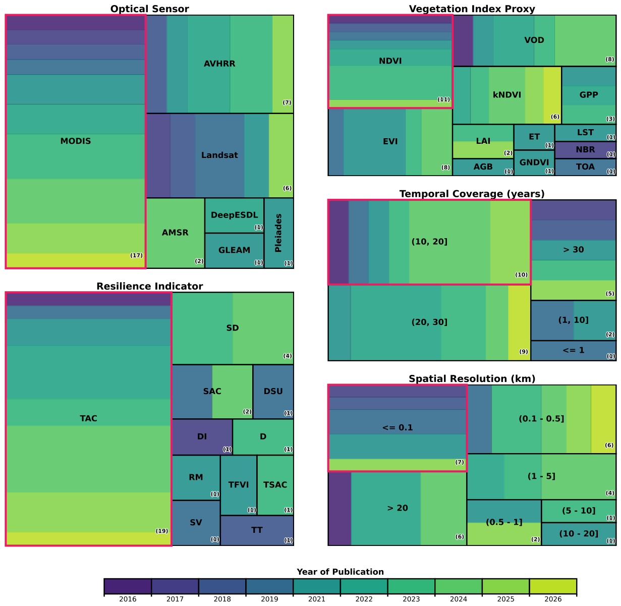
Figure 6.
Temporal trends in mean NDVI from 1984 to 2024 over the Eastern Canadian Shield Taiga. The compared timeseries were derived using a GeoMedian composite strategy, for both the uncalibrated and calibrated version using the coefficients derived for the eastern Canadian boreal forest. The pairwise Theil–Sen slope difference between the approaches (+0.0017) indicates a significant (p < 0.001) divergence of the trend magnitudes. The shaded regions correspond to periods of sensor shifts.
Figure 6.
Temporal trends in mean NDVI from 1984 to 2024 over the Eastern Canadian Shield Taiga. The compared timeseries were derived using a GeoMedian composite strategy, for both the uncalibrated and calibrated version using the coefficients derived for the eastern Canadian boreal forest. The pairwise Theil–Sen slope difference between the approaches (+0.0017) indicates a significant (p < 0.001) divergence of the trend magnitudes. The shaded regions correspond to periods of sensor shifts.
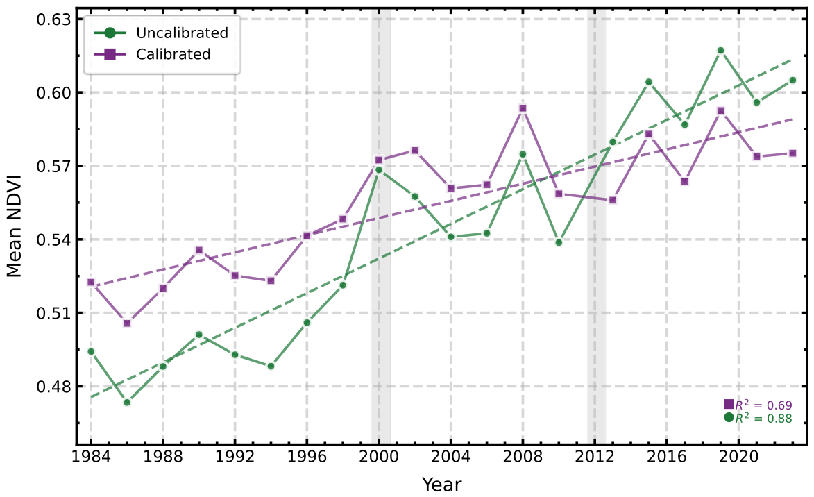
Disclaimer/Publisher’s Note: The statements, opinions and data contained in all publications are solely those of the individual author(s) and contributor(s) and not of MDPI and/or the editor(s). MDPI and/or the editor(s) disclaim responsibility for any injury to people or property resulting from any ideas, methods, instructions or products referred to in the content. |
© 2026 by the authors. Licensee MDPI, Basel, Switzerland. This article is an open access article distributed under the terms and conditions of the Creative Commons Attribution (CC BY) license (http://creativecommons.org/licenses/by/4.0/).
Copyright: This open access article is published under a Creative Commons CC BY 4.0 license, which permit the free download, distribution, and reuse, provided that the author and preprint are cited in any reuse.