
Submitted:
09 October 2026
Posted:
10 October 2026
You are already at the latest version
Abstract
In this study, the numerical comparison is performed in solving first-order neutrosophic initial value problems employing two algorithms, namely, the Euler and fourth-order Runge-Kutta (RK4) methods in the neutrosophic environment. As an example of such kind of problem, the model y^' (t)=0.5∙y(t) on [0,2] is chosen, but in the case of the additional neutrosophic initial condition y(0)=⟨(0.8,1.0,1.3)⟩. This problem is represented as crisp-endpoint systems by means of ( α,β,γ )-cut approach, and then, it is solved numerically at each cut level while using exact solution as a reference. In accordance with the iteration results, the maximum absolute error of the Euler algorithm at h=0.2 is 1.619×10^(-1) at point t=2, whereas for the RK4 approach, this value is 2.7×10^(-6), meaning that the improvement degree reaches about five orders of magnitude. The analysis of step refinement confirms the convergence orders of the methods that are 1.00 and 4.00 for the Euler and RK4 approaches, respectively.
Keywords:
neutrosophic set
; neutrosophic differential equation
; ( α
; β
; γ )-cut
; Euler method
; Runge-Kutta method
; convergence order
; neutrosophic normed space
; functional analysis
1. Introduction
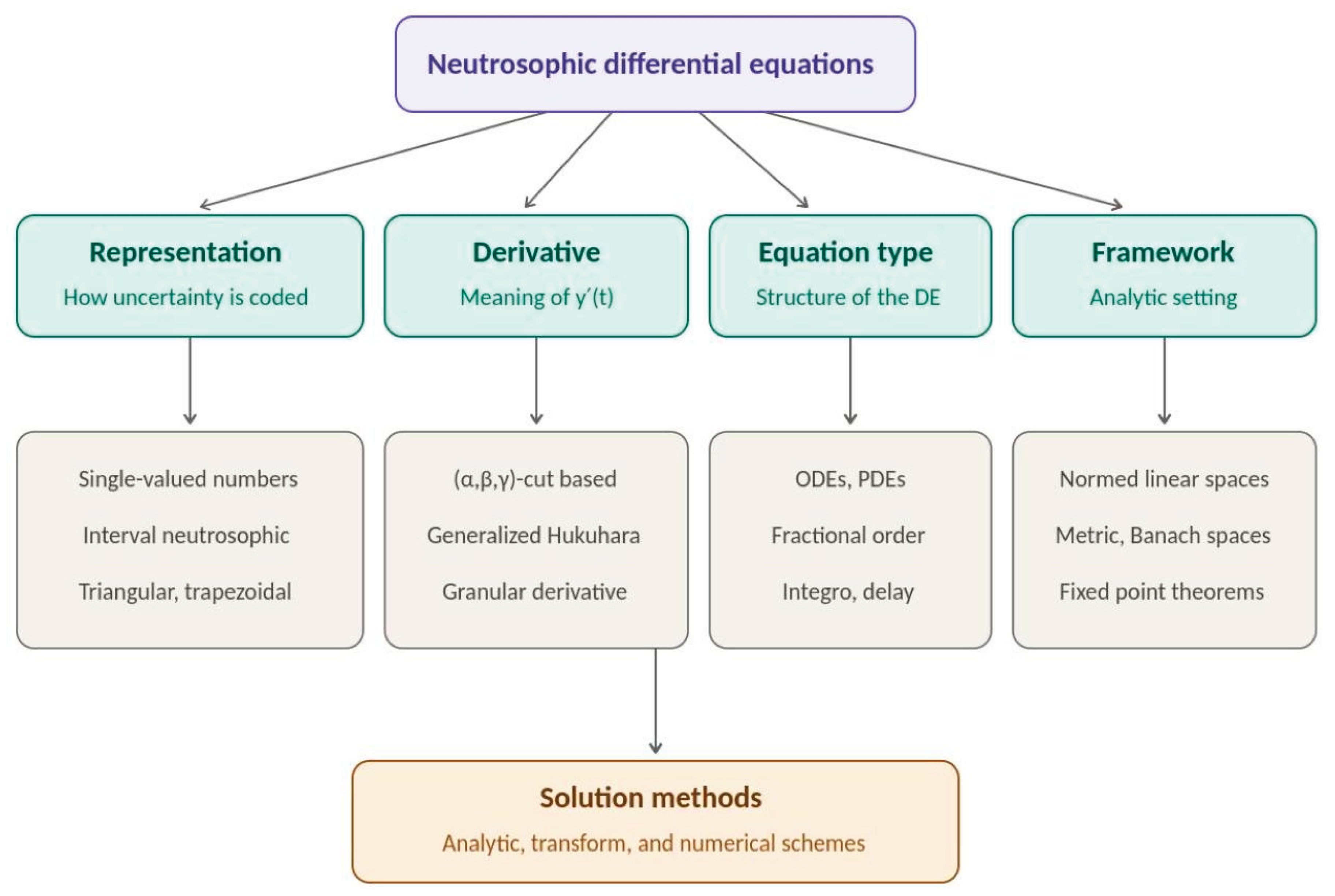
Models of realistic processes in nature do not usually have perfectly known data. Measurement errors, imprecision of judgements of experts and lack of determination in many practical applications lead to the situation when some of the information is not determined at all: either true or false. The classical theory of differential equations presupposes crisp initial data and crisp coefficients and therefore cannot model this situation. In the theory of fuzzy sets formulated by Zadeh in 1965, this type of information was represented by means of one degree of belonging to an element, which gave rise to the development of the theory of fuzzy differential equations. After that, the theory of intuitionistic fuzzy sets, suggested by Atanassov, offered a more elaborate interpretation of this idea by adding the degree of non-belonging to an element.. Nevertheless, even such an elaborated description remains indeterminate and supplements the existing information. The theory of neutrosophic sets was introduced by Smarandache [1], and the theory of single-valued neutrosophic sets was introduced by Wang et al [2]. Here, each component is defined through three independent degrees of membership namely the degree of truth , degree of indeterminacy and degree of falsity , such that . This makes indeterminacy a separate and independent value and not a complementary value anymore. This extra degree of freedom is highly important in handling conflicting, incomplete and doubtful information that exists regularly in the fields of population dynamics, epidemiology, electrical circuits, decision making etc. Neutrosophic limit, neutrosophic derivative and neutrosophic integral were introduced in [3] by Smarandanche. One may note that the development of the theory of differential equations in neutrosophic set setting is due to the papers written by Sumathi and Mohana Priya [4]. In particular, they introduced the notion of neutrosophic differential equation using the neutrosophic number form of the initial condition and its cuts: one cut for the truth membership function, one cut for the indeterminacy membership function and one cut for the falsity membership function. Thus, each cut transforms the neutrosophic problem into the pair of crisp endpoint problems, and the whole solution becomes a family of nested intervals parametrized by the three levels. The approach was generalized to the trapezoidal neutrosophic data in [5], to second-order boundary-value problems in [6], where a special concept of neutrosophic derivative was introduced, and to granular neutrosophic fractional models in control theory in [8]. Arithmetic and ranking of single-valued neutrosophic numbers .[necessary to interpret the computed solutions are provided by Deli and Şubaş [12].It is well known that a numerical algorithm is reliable if the original problem is well posed, and this is where functional analysis comes into play. Bera and Mahapatra constructed neutrosophic linear spaces and defined thereon the neutrosophic norm [9,10], producing a graded version of the normed linear space, where notions like convergence, Cauchy sequence and completeness are meaningful. Neutrosophic metric spaces and corresponding theorems of Baire categories and uniform limits are introduced by Kirişci and Şimşek [11]. For the family of complete neutrosophic metric spaces, the initial value problem reduces to the fixed-point problem for the related integral operator, and methods of Banach type contractive mappings give us the uniqueness and existence of the neutrosophic solution. These results assure that the systems of endpoint problems produced by the cut decomposition represent true neutrosophic-number.valued solutions, which is the property our computations should conserve.The above landscape can be visualized as in Figure 1, where neutrosophic differential equations are classified according to four axes: uncertainty representation, derivative concept, type of the equation and functional-analytic framework, all four determining the choice of solution method. The current paper follows one of the paths of this classification: triangular single-valued neutrosophic initial data, -cut approach to the derivative, first-order linear ordinary equation and neutrosophic normed space framework for well-posedness. Our contribution is computational: We consider two one-step integration schemes, namely the neutrosophic Euler scheme and the neutrosophic fourth-order Runge-Kutta scheme on a test problem with an exact solution and analyze them through an iteration table, convergence analysis and plotting of the neutrosophic solution. The remainder of this research paper is structured as follows: Problem statement in Section 2, literature review on both approaches in Section 3, numerical results and their discussion in Section 4, their implications in Section 5, and conclusion in Section 6.
Figure 1 is interpreted from top to bottom. Starting from the root node, neutrosophic differential equations split into four classification axes presented as the middle row. The first one is called Representation, which is responsible for the method of representing the uncertainty in the data set. The most used types are single valued neutrosophic number, interval neutrosophic number, and triangular/trapezoidal shape; triangular shape will be used in this research. The second axis, Derivative, defines the notion of the derivative of a neutrosophic-valued function and includes three possible variants: -cuts approach used in this study, generalized Hukuhara differentiability, and granular derivative. The third axis, Equation type, indicates the nature of the equation itself: it can be ordinary or partial, of fractional order, integrodifferential, or delay. Finally, the last axis, Framework, indicates the functional-analytic environment where well-posedness of the problem is established: neutrosophic normed linear spaces, neutrosophic metric and Banach spaces, and the fixed point theorems valid therein. The arrow from all axes to the bottom node, Solution methods, illustrates that a particular solution technique, analytical, transform-based, or numerical, is determined only after choosing one option on all axes; Euler and Runge-Kutta methods discussed in this .paper are examples of the latter category
2. Problem formulation
This study the first-order linear neutrosophic initial value problem
where the initial state is the triangular single-valued neutrosophic number
with . Following [1,2], the three membership functions of are independent; for the triangular form used here they are given by
otherwise
so that the truth degree peaks at the core while the indeterminacy and falsity degrees vanish there and grow toward the endpoints of the support .
The computational form of the problem is obtained through the -cut of introduced in [4]. For a truth level the truth cut is the closed interval
while the indeterminacy cut at level and the falsity cut at level widen from the core toward the support:
Applying the truth cut to problem (1) converts it, on every level , into the pair of crisp endpoint initial value problems
and analogously for the - and -cuts. Since , the lower and upper equations in (6) decouple and each admits the exact solution
The exact solution (7) is considered as the benchmark solution to test the performance of the numerical methods; the neutrosophic solution of (1) is obtained through the aggregation of the intervals , y_u(t; ] for all the levels of cuts, and the validity of this approach is ensured from the fixed point theory in complete neutrosophic normed/metric spaces [9,10,11].
3. The two methods
Let , and for . Both approaches provide approximate solutions of for all the functions at both end points as defined in equation (6), using the initial conditions y_I(0; ) and y_u( ). The neutrosophic Euler approach advances the endpoints by
and has local truncation error and global order one. Method 2, the neutrosophic fourth-order RungeKutta method (RK4), uses the classical four-stage rule
with local truncation error and order four globally. Each step of RK4 needs four function evaluations of the RHS f compared to just one in the case of Euler's method. Accuracy is determined by the maximum :absolute error at the end point of each grid and the convergence order is calculated using :
Both quantities are reported in Section 4 for the widest truth cut , on which the initial interval [0.8, 1.3] is largest and the numerical error is most visible.
3.1. Algorithms
The entire computation process is described in Algorithm 1 and Algorithm 2. The first algorithm is the cutdecomposition procedure: it accepts the neutrosophic equation, cut levels, and the selected one-step method M , and outputs the trajectory endpoints that form the neutrosophic solution. The second algorithm is the comparison procedure used in this work: it executes the first algorithm with Euler and methods, compares the results with the exact solution (7), and generates tables and graphs .presented in Section 4
| Algorithm 1. Cut-decomposition solver for the neutrosophic IVP (1) with method M∈{Euler, RK4} |
| Input: k, T, N; neutrosophic number à = ; cut levels L = {ℓ₁, …, ℓ_m}; method M Output: endpoint trajectories y_l(t_n; ℓ), y_u(t_n; ℓ) for all n = 0, …, N and all ℓ L 1: h ← T / N; t_n ← n·h for n = 0, …, N 2: for each cut level ℓ L do 3: compute the initial interval [y_l⁰, y_u⁰] by (4) for a truth cut, or by (5) for an indeterminacy or falsity cut 4: for each endpoint y⁰ {y_l⁰, y_u⁰} do 5: y₀ ← y⁰ 6: for n = 0 to N − 1 do 7: if M = Euler then y_{n+1} ← y_n + h·f(t_n, y_n) ► rule (8) 8:else compute k₁, k₂, k₃, k₄ and y_{n+1} ← y_n + (h/6)(k₁ + 2k₂ + 2k₃ + k₄) ► rule (9) 9: end for 10: end for 11: if y_l(t_n; ℓ) ≤ y_u(t_n; ℓ) for all n, assemble the band [y_l(t_n; ℓ), y_u(t_n; ℓ)] 12: end for 13: return all endpoint trajectories |
| Algorithm 2. Comparison protocol for the two neutrosophic methods |
| Input: problem data of Algorithm 1; iteration step count N = 10; refinement counts N {5, 10, 20, 40, 80, 160, 320}; exact solution (7) Output: iteration table (Table 1); convergence table (Table 2); Figure 2, Figure 3, Figure 4 and Figure 5 1: run Algorithm 1 at the truth cut α = 0 with N = 10, once with M = Euler and once with M = RK4 2: for n = 0, …, N record both endpoint values and the exact values (7); compute E_n^M ← max( |y_{l,n} − y_l(t_n)| , |y_{u,n} − y_u(t_n)| ) for M ∈ {Euler, RK4} → Table 1 3: for each refinement count N_j do 4: h_j ← T / N_j; run both methods on the upper endpoint; compute the maximum error E^M(h_j) by (10) 5: end for 6: p_obs^M ← log₂( E^M(h_j) / E^M(h_{j+1}) ) for consecutive steps → Table 2 7: solve on all cut levels with M = RK4 and plot the solution bands, the membership surface,the per-iteration errors, and the log–log convergence diagram → Figure 2, Figure 3, Figure 4 and Figure 5 8: return tables and figures |
Two comments regarding the algorithms. Firstly, the structure test in line 11 of Algorithm 1 is never triggered in the tests since for the growth equation, both methods guarantee that the order of the end points is preserved so that the resulting intervals form well-defined neutrosophic cuts, as expected from the well-posedness theory in neutrosophic normed spaces [9,10,11]. Secondly, the cost of each step of the two methods is different only in the number of evaluations of (one in case of Euler method in line 7, four for RK4 in line 8), so that Algorithm 2 allows comparing the accuracy at an equal number of steps; hence, the difference in accuracy discussed in Section 4 underestimates the RK4 superiority by a factor of at most four in .
4. Numerical results
4.1. Iteration Table
Iteration history for (full) is presented in Table 1 using iterations (step ). The trajectories and exact solutions for both endpoints, as well as the maximal error for the methods at the endpoints, are .shown

Table 1.
Iteration results at the truth cut for .
| iter | t | Euler lower | Euler upper | RK4 lower | RK4 upper | Exact lower | Exact upper | Euler abs err | RK4 abs err |
|---|---|---|---|---|---|---|---|---|---|
| 0 | 0.00 | 0.800000 | 1.300000 | 0.800000 | 1.300000 | 0.800000 | 1.300000 | 0.000e+0 | 0.000e+0 |
| 1 | 0.20 | 0.880000 | 1.430000 | 0.884137 | 1.436722 | 0.884137 | 1.436722 | 6.722e-3 | 1.100e-7 |
| 2 | 0.40 | 0.968000 | 1.573000 | 0.977122 | 1.587823 | 0.977122 | 1.587824 | 1.482e-2 | 2.400e-7 |
| 3 | 0.60 | 1.064800 | 1.730300 | 1.079887 | 1.754816 | 1.079887 | 1.754816 | 2.452e-2 | 4.000e-7 |
| 4 | 0.80 | 1.171280 | 1.903330 | 1.193459 | 1.939372 | 1.193460 | 1.939372 | 3.604e-2 | 5.900e-7 |
| 5 | 1.00 | 1.288408 | 2.093663 | 1.318977 | 2.143337 | 1.318977 | 2.143338 | 4.967e-2 | 8.200e-7 |
| 6 | 1.20 | 1.417249 | 2.303029 | 1.457694 | 2.368753 | 1.457695 | 2.368754 | 6.573e-2 | 1.090e-6 |
| 7 | 1.40 | 1.558974 | 2.533332 | 1.611001 | 2.617877 | 1.611002 | 2.617879 | 8.455e-2 | 1.410e-6 |
| 8 | 1.60 | 1.714871 | 2.786665 | 1.780432 | 2.893201 | 1.780433 | 2.893203 | 1.065e-1 | 1.770e-6 |
| 9 | 1.80 | 1.886358 | 3.065332 | 1.967681 | 3.197482 | 1.967682 | 3.197484 | 1.322e-1 | 2.210e-6 |
| 10 | 2.00 | 2.074994 | 3.371865 | 2.174624 | 3.533764 | 2.174625 | 3.533766 | 1.619e-1 | 2.710e-6 |
4.2. Convergence Study
In Table 2, the max errors on the upper end point over are shown for when the step size goes from to and the order calculated using base-2 logs of the ratios of errors.
Table 2.
Maximum error versus step size and observed convergence orders.
| h | Euler max err | RK4 max err | Euler order | RK4 order |
|---|---|---|---|---|
| 0.40000 | 2.990e-1 | 3.990e-5 | — | — |
| 0.20000 | 1.619e-1 | 2.710e-6 | 0.885 | 3.880 |
| 0.10000 | 8.448e-2 | 1.765e-7 | 0.938 | 3.940 |
| 0.05000 | 4.318e-2 | 1.127e-8 | 0.968 | 3.970 |
| 0.02500 | 2.184e-2 | 7.115e-10 | 0.984 | 3.985 |
| 0.01250 | 1.098e-2 | 4.470e-11 | 0.992 | 3.992 |
| 0.00625 | 5.506e-3 | 2.804e-12 | 0.996 | 3.995 |
4.3. Description of the Computed Results
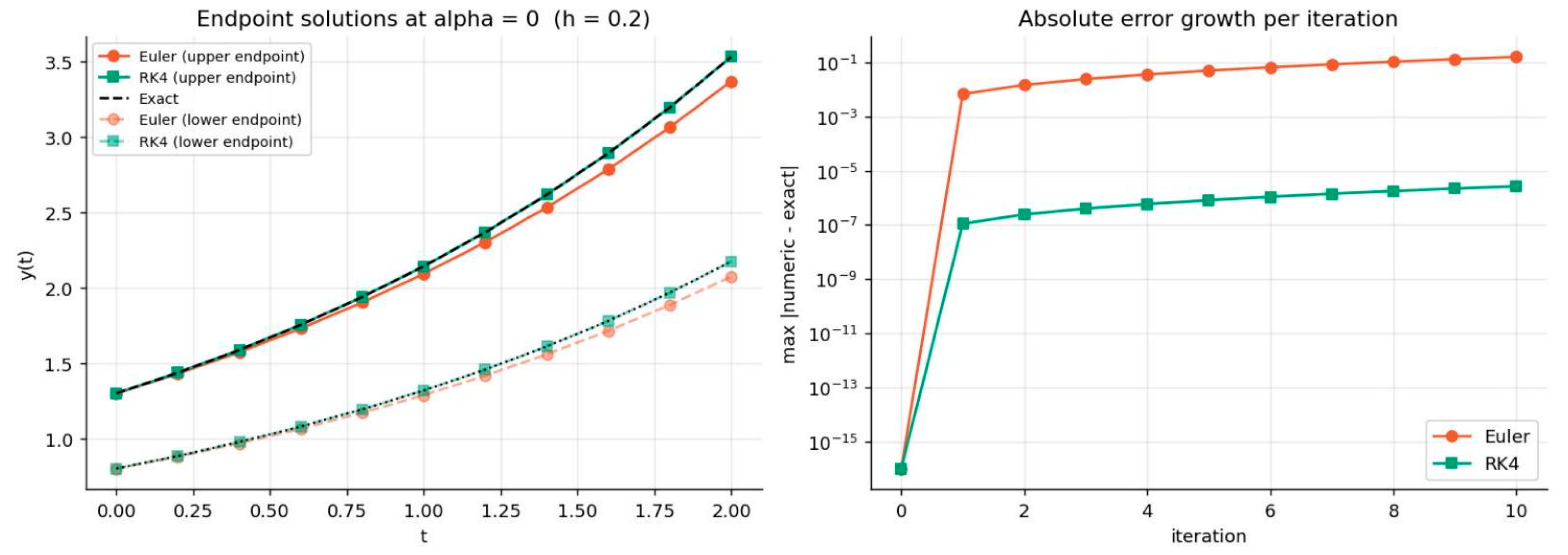
In turn, the numerical results can be interpreted in detail as follows. (i) Accuracy at each iteration. Starting from the exact interval the Euler iterates become increasingly smaller than the exact endpoint values since this method traces the tangent line of an exponentially convex solution; thus, by the end of iteration the exact upper endpoint is 2.143338 , whereas Euler reaches the value of 2.093663, the absolute error being , and at the end of iteration the exact value 3.533766 is approximated as 3.371865 , i.e., the absolute error equals , which is about of the exact value. The RK4 iterates coincide with the exact values up to six decimal digits for the first three iterations and differ only by at the final time, that is, about . (ii) Growth of errors. The errors increase monotonically with , as was to be expected for the growth equation, however, in the logarithmic scale of Figure 4 the two curves are parallel; the errors of the methods have the same growth mechanism (proportional to the solution) but differ by an almost constant factor of about in favor of RK4. (iii) Order of convergence. Decreasing twice, the Euler error is reduced by a factor tending to 2 (order changes ), whereas RK4 error is reduced by a factor tending to 16 (order changes ); at the finest step the error of RK4, , tends to the limit of doubleprecision arithmetic. (iv) Geometry of neutrosophic solution. At each time step the lower endpoint stays below the upper endpoint at all cut levels, the bands are nested within the cut level, and the support width increases exponentially from 0.5 at up to 1.36 at (see Figure 2 and Figure 3); consequently, the calculated solution represents a proper triangular neutrosophic number at all times during the integration, and both methods preserve the geometry needed for the fixed point theory in neutrosophic Banach spaces [9,10,11].
4.4. Graphical Results
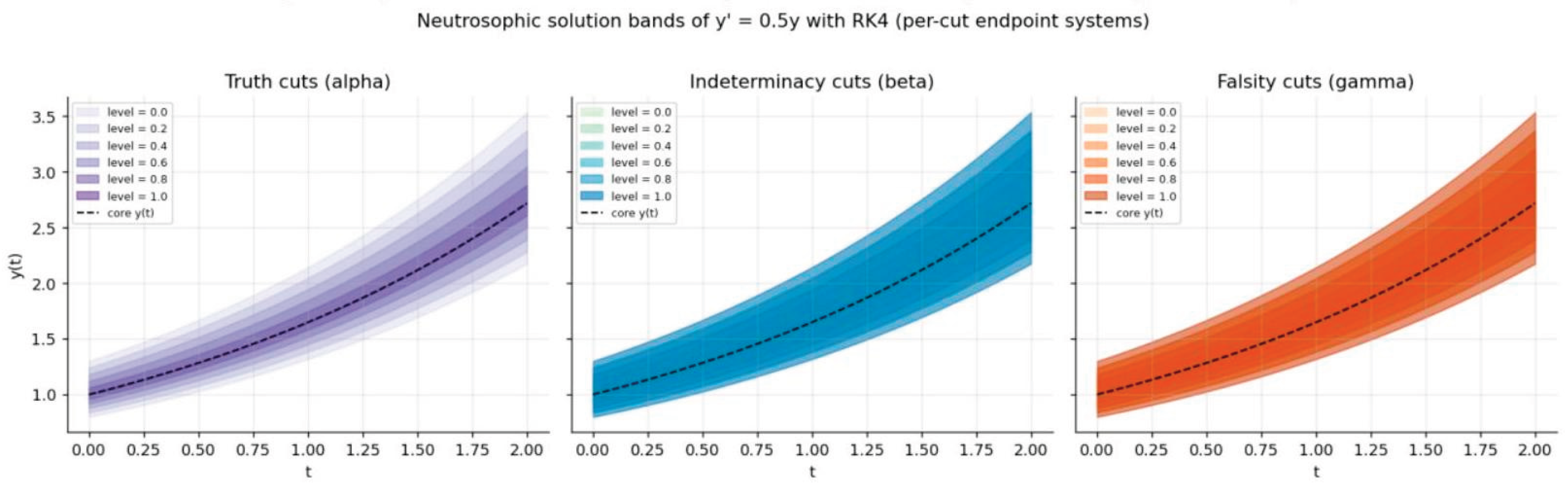
Figure 2 depicts the neutrosophic solution found using RK4 in the form of bands at six stages of truth, indeterminacy, and falsity cuts. Bands grow exponentially with time in relation to the central solution, indicating the spread of indeterminacy from the start point throughout the process.
Figure 2.
Neutrosophic solution bands of under truth, indeterminacy, and falsity cuts (RK4).
The plot on the left hand side of Figure 3 represents the truth membership surface for the solution, in which for any t value the cross section is represented by the triangle shape membership of . The heat map on the right hand side represents the width of support as a function of and
Figure 3.
Truth-membership surface of and propagation of the uncertainty width.
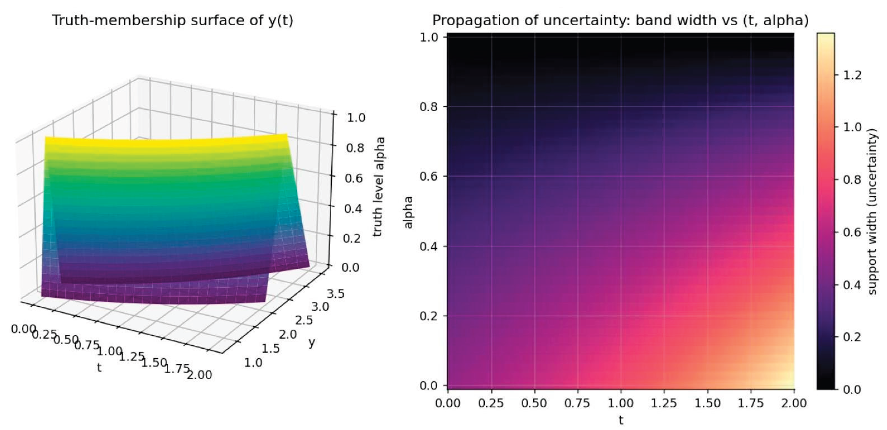
Figure 4 shows a comparison between the end-point trajectories for both methods with respect to the exact solution and also traces the maximal absolute error per step in a log plot. It is clear that the Euler curve diverges from the exact solution while the RK4 points are aligned with it.
Figure 4.
Endpoint solutions at (left) and per-iteration maximum absolute error (right).
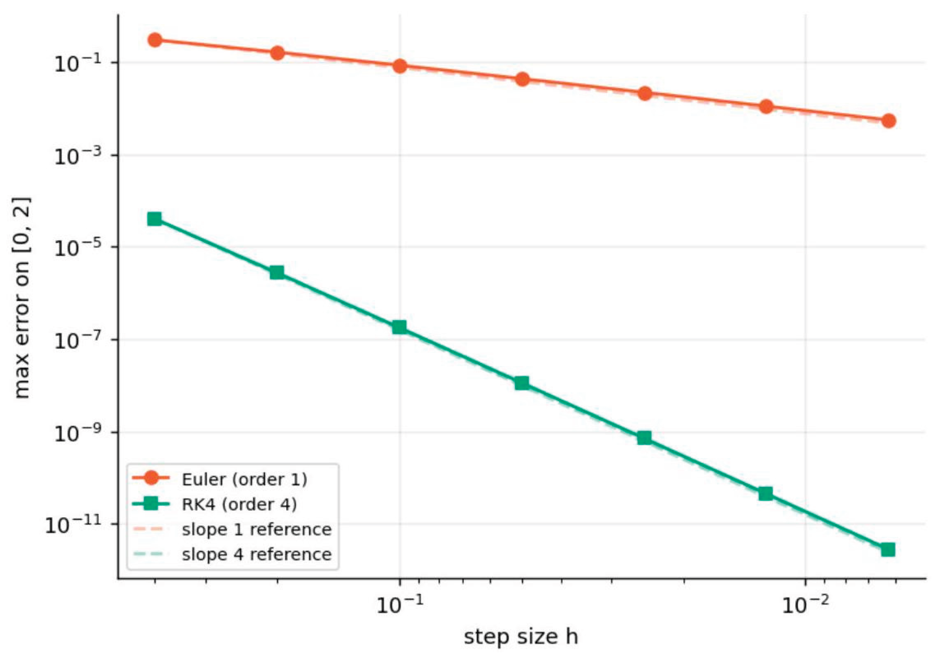
The diagram of the convergence for Figure 5 is provided on the log-log scale along with reference lines of slope one and four. The calculated error plots coincide with the reference slopes in all ranges of the step size, which indicates first order convergence of the neutrosophic Euler method and fourth order convergence of neutrosophic RK4. Convergence of the two neutrosophic methods
Figure 5.
Convergence of the two methods with slope-1 and slope-4 reference lines.
5. Discussion
These are the three main findings from the simulations. Firstly, the cut-decomposition technique carries over the accuracy theory of classical one-step methods into the context of neutrosophic calculus intact: the orders of accuracy are identical in theory and in practice on each cut. Secondly, for the same step size, the RK4 scheme is immensely more accurate: at its absolute error is nearly times smaller than that of Euler's method, significantly outstripping the latter's quadruple expense per step. Alternatively, the former would need a step size several thousands of times smaller in order to achieve the accuracy of the latter with . Lastly, the geometry of the neutrosophic solution is retained by both numerical techniques: the lower and upper bounds never intersect, thus ensuring that the bands calculated stay properly defined neutrosophic numbers at each step, as expected from well-posedness proved using fixed point theory in neutrosophic spaces [9,10,11].
6. Conclusion
In the case of neutrosophic initial value problems of first order that can be decomposed by -cuts, the neutrosophic Runge-Kutta 4 scheme outperforms the neutrosophic Euler scheme; the former has an extra five significant digits of accuracy and clear fourth order of convergence at reasonable step sizes. The approach applies in a straightforward manner to nonlinear functions on the right-hand side, decay problems with generalized Hukuhara type-(i)/(ii) branching, and neutrosophic fractional differential equations [8].
Appendix A. Computational Details
All calculations were carried out in Python 3 using NumPy, pandas, and Matplotlib libraries. The source code is fully provided (neutrosophic_comparison.py) to create the class of a triangular neutrosophic number and implement three cut operations, two integrators, as well as functions producing Table 1 and Table 2 and Figure 2, Figure 3, Figure 4 and Figure 5. The following model parameters are used: iterations for Table, and
References
- Smarandache, F. A Unifying Field in Logics. In Neutrosophy: Neutrosophic Probability, Set and Logic; American Research Press: Rehoboth, 1999. [Google Scholar]
- Wang, H.; Smarandache, F.; Zhang, Y. Q.; Sunderraman, R. Single valued neutrosophic sets. Multispace Multistructure 2010, 4, 410–413. [Google Scholar]
- Smarandache, F. Neutrosophic Precalculus and Neutrosophic Calculus; EuropaNova: Brussels, 2015. [Google Scholar]
- Sumathi, I. R.; Mohana Priya, V. A new perspective on neutrosophic differential equation. Int. J. Eng. Technol. 2018, 7(4.10), 422–425. [Google Scholar] [CrossRef]
- Sumathi, I. R.; Antony Crispin Sweety, C. New approach on differential equation via trapezoidal neutrosophic number. Complex Intell. Syst. 2019, 5, 417–424. [Google Scholar] [CrossRef]
- Moi, S.; Biswas, S.; Pal, S. Second-order neutrosophic boundary-value problem. Complex Intell. Syst. 2021, 7, 1079–1098. [Google Scholar] [CrossRef] [PubMed]
- Moi, S.; Biswas, S.; Pal, S. Neutrosophic linear differential equation with a new concept of neutrosophic derivative. In Neutrosophic Operational Research; Smarandache, F., Abdel-Basset, M., Eds.; Springer: Cham, 2021. [Google Scholar]
- Son, N. T. K.; Dong, N. P.; Long, H. V.; Khastan, A. Linear quadratic regulator problem governed by granular neutrosophic fractional differential equations. In ISA Transactions; 2019. [Google Scholar]
- Bera, T.; Mahapatra, N. K. On neutrosophic soft linear spaces. Fuzzy Inf. Eng. 2017, 9, 299324. [Google Scholar] [CrossRef]
- Bera, T.; Mahapatra, N. K. Neutrosophic soft normed linear spaces. Neutrosophic Sets Syst. 2018, 23, 52–71. [Google Scholar]
- Kirişci, M.; Şimşek, N. Neutrosophic metric spaces. Math. Sci. 2020, 14, 241–248. [Google Scholar] [CrossRef]
- Deli, I.; Şubaş, Y. A ranking method of single valued neutrosophic numbers and its applications to multiattribute decision making problems. Int. J. Mach. Learn. Cybern. 2017, 8(4), 1309–1322. [Google Scholar] [CrossRef]
Figure 1.
Classification of neutrosophic differential equations in functional analysis.
Disclaimer/Publisher’s Note: The statements, opinions and data contained in all publications are solely those of the individual author(s) and contributor(s) and not of MDPI and/or the editor(s). MDPI and/or the editor(s) disclaim responsibility for any injury to people or property resulting from any ideas, methods, instructions or products referred to in the content. |
© 2026 by the authors. Licensee MDPI, Basel, Switzerland. This article is an open access article distributed under the terms and conditions of the Creative Commons Attribution (CC BY) license (http://creativecommons.org/licenses/by/4.0/).
Copyright: This open access article is published under a Creative Commons CC BY 4.0 license, which permit the free download, distribution, and reuse, provided that the author and preprint are cited in any reuse.