
Submitted:
09 October 2026
Posted:
10 October 2026
You are already at the latest version
Abstract
This article examines issues related to determining the resolution in multichannel post-detector nonparametric signal detectors. We define resolution as the ability to distinguish closely spaced targets. Typically, theoretical studies examine the effectiveness of detecting a single useful signal in one of the Cell Under Test consistent with its informative parameters. However, in real systems, the number of useful signals can be large. Consequently, determining the ability to detect multiple signals is an extremely important task. This article discusses a method for determining resolution based on an analysis of the uncertainty function for Wilcoxon’s rank statistics.
Keywords:
resolution
; nonparametric signal detection
; reference cells
; uncertainty function
; multichannel detec-tion systems
; directional pattern
1. Introduction
In radio engineering systems, signal discrimination refers to the ability to distinguish between closely spaced targets, i.e., to distinguish between signals from two closely spaced “resolution cells” [1]. By “resolution cell,” we mean a region in the signal parameter space whose center corresponds to the tuning parameters of a given detection channel, and whose dimensions along the coordinate axes correspond to the sizes of the uncertainty regions for the respective parameters [2]. In this context, resolution implies the ability to distinguish between two targets both in terms of range () and radial velocity (). Thus, the resolution problem reduces to the problem of separately detecting two signals. In other words, it is necessary to determine whether one or two signals are present in the received signal.
The received useful signal has a specific spatial-temporal and polarization structure; therefore, resolution is considered in terms of spatial, temporal, and polarization parameters [3]. The spatial structure of the signal depends on its direction of arrival; therefore, in this case, resolution is considered in terms of bearing and elevation angle. The temporal structure of the signal depends on the time delay and the frequency shift (Doppler frequency) of the signal. Therefore, resolution is considered in terms of the time delay and frequency shift of the signals. Resolution is quantitatively characterized by the minimum difference in a resolvable parameter between two signals at which they can still be distinguished [4]. Time-delay resolution is the minimum difference in the time delays of two signals with the same frequency shift and arrival direction at which they are still observed separately, i.e., they differ. The frequency-shift resolution of signals is the minimum difference in frequency shift between two signals having the same time delay and direction of arrival at which they are still observed separately. The resolution in the direction of signal arrival is the minimum angle between the directions of two signal sources having the same time delay and frequency shift at which they can still be distinguished.
Some theoretical considerations are presented below.
The basis for signal detection is the calculation of the autocorrelation function, which is described in detail in many textbooks on radar. The technical implementation is carried out using correlation detectors [5,6,7,8] or matched filters [9,10], which are commonly referred to in the literature as optimal signal processing devices. The output of the optimal signal processing device is a modulated signal, whose envelope can be schematically represented as a simple radio pulse with a duration of (Figure 1).
The maximum signal value corresponds to . In this case, the permissible deviation in the resolvable parameter is selected as 0.5 times the maximum value and corresponds to the signal duration , i.e., . Consequently, to quantitatively evaluate signal detection, it is necessary to derive an expression that describes the signal envelope at the output of the optimal processing device along the axis of the resolved parameter and to estimate its width based on 0.5 times the maximum value.
Signals are distinguished based on the shape of the output voltage from the optimal processing device. Figure 2 shows the envelopes of the two signals observed at the output of the optimal processing device.
The -axis shows values of the parameter (delay time or shift frequency), which distinguish the signals. Analysis of the figures (Figure 2, ) shows that, for the same difference Δ, signals with a narrower output envelope width from the optimal processing devices are more easily distinguished. In Figure 2, , the signals are practically indistinguishable in terms of the parameter . Consequently, the shape of the output signals from the optimal processing device has the most significant effect on the resolution. The maximum achievable resolution is referred to as the potential resolution.
2. Theoretical Foundations of Signal Detection and Discrimination
In radar, when detecting signals against a background of interference, the entire sampling space is divided into two main parts: the signal cell and the reference cell (window) [11]. Signal cell - the element under test (often referred to as the Cell Under Test or CUT). This is a specific resolution cell (in range or Doppler) in which the presence of a target is currently being checked. Data from this resolution cell is compared to a threshold. If the value in it exceeds the threshold, a decision is made to detect a target. Reference cell - the surrounding resolution “cells” used to assess the “background.” This is a group of cells surrounding the signal cell (to the left and right in range or Doppler). The average power of interference or noise at that moment is calculated based on these cells. Based on this cell (window), the system adaptively sets the detection threshold.
As noted above, the main approach to signal discrimination is based on analyzing the envelope of the output signals from the optimal processing device, which represents the autocorrelation function of the signals; its normalized value is referred to in the literature as the uncertainty function (UF) [12,13,14]. The mathematical operation involved in calculating the AF is the computation of the cross-correlation integral between the expected signal and the received signal , which is shifted relative to by a time [15]:
Consider signal discrimination using a nonparametric signal detection method based on the Wilcoxon rank statistic [16,17,18]. It is well known that nonparametric signal detection methods are used when the statistical properties of the received signal are unknown in advance [19,20].
The receiving path contains a set of channels tuned to different signal arrival angles , where = 1, …, is the channel number; is the number of channels. The preprocessing block (PB), which precedes the ranking block (RB), is constructed according to the standard filter-detector (F-D) scheme. The output voltage of the -th channel of the detector, is quantized with a step size of . The set of samples is divided into “resolution cells” based on the signal arrival time , where k is the number of the current range sample (strobe).
Since the receiving path is multichannel with respect to two informative parameters of the received signal - time and direction of arrival - the circuit allows for two ranking methods:
temporal (Figure 3), in which the rank of the -th sample () in the -th spatial channel is calculated by comparing it with the - time-adjacent samples () of the same spatial channel, located to the left and right of the k-th range sample
spatio-temporal (Figure 4), in which ranks are formed from the readings of neighboring spatial channels (c and b) within the current range strobe,
Both algorithms (2) and (3) correspond to ranking based on the overall reference sample.
The set of ranks is fed to the rank statistic calculator (RSC) whose value is compared with the threshold in the thresholding device (TD). Based on the results of this comparison, a decision is made regarding the presence or absence of a signal in the current “resolution cell”.
Consider the traditional approach to discriminating between two signals based on the uncertainty function for both temporal and spatio-temporal ranking methods.
3. Signal Discrimination Using the Uncertainty Function in the Temporal Ranking Method
According to the generally accepted definition [21], which follows from (1), the uncertainty function of a given processing algorithm (where is an array of observed data, and is the vector of information parameters of the expected signal ), is defined as the normalized value of the increment in the mathematical expectation caused by the arrival of the signal , i.e.,
where is the true value of , and denotes the sign of the mathematical expectation.
We analyze expression (4) for the Wilcoxon rank statistic
Let the direction of the signal arrival coincide with the direction of the beam pattern (BP) orientation of the -th spatial channel, and let the arrival time differ from the expected time . Suppose that a receiver path with a temporal ranking algorithm is used to detect the signal. Then, for the Wilcoxon statistic, taking into account expressions (2) and (5), we obtain
Since the signal is contained only in the samples numbered , when , a portion of its samples falls within the reference cell numbered . On the other hand, the signal is absent in the samples of the signal cell with indices [k, k0 - 1]. Consequently, instead of (6), we can write
where and are the voltage readings at the output of the -th spatial channel, respectively, in the absence and presence of a signal at the input of the receiving path.
If the measurements are independent of one another and statistically homogeneous, then
where is the distribution function of the observed data .
From expression (8), we obtain expressions for the mathematical expectation of the rank statistic (6) when a signal is present and when it is absent (expressions (9) and (10), respectively):
Taking these expressions into account, formula (4) takes the form
After normalizing to the maximum value, we obtain the uncertainty function
Similarly, the uncertainty function can be derived for other values of . After performing the appropriate transformations, we obtain an expression for the uncertainty function of the Wilcoxon statistic under time-based ranking
This expression holds for an arbitrary voltage distribution . It follows from equation (13) that as the size of the reference cell increases,
which corresponds to the uncertainty function of a traditional sum-of-squares integrator [22,23].
Equation (14) also holds for the space-time ranking method, but only for an orientation of the BP in which the maximum of the -th channel’s BP corresponds to zeros in the BP of the other channels [24].
Figure 5 shows the uncertainty function of the traditional sum-of-squares integrator (red) and the Wilcoxon rank detector (green) for т = 20, .
The Wilcoxon detector’s uncertainty function is somewhat sharper than that of a traditional sum-of-squares integrator; that is, the resolution of the Wilcoxon statistic for n < 5 is better than that of a traditional sum-of-squares integrator. When n > 5, the uncertainty function of the Wilcoxon statistic has a negative component caused by the signal falling within the reference cell, which leads to a deterioration in the resolution of the Wilcoxon statistic compared to the traditional sum-of-squares integrator. Figure 6 shows the uncertainty function for two signals separated in time by . It can be seen from Figure 6 that the interval is a cutoff interval. When , the signals are indistinguishable. The signals can only be distinguished when . For example, the signals are clearly distinguishable when (Figure 7).
4. Signal Discrimination Using the Uncertainty Function in the Spatial-Temporal Ranking Method
For the spatial-temporal ranking method (3), the Wilcoxon statistic will be
from which
It is known [25] that in post-detector detection systems, the distribution function of the observed data follows a Rayleigh distribution [26]
where and are the variances of the interference and the random signal, respectively.
Substituting (17) into (16) and integrating, we obtain
where and are the signal variances in the -th and -th spatial channels, respectively.
Taking this expression into account, expression (4) for the spatial-temporal ranking will take the form
After normalizing to the maximum value, we obtain the uncertainty function for spatial-temporal ranking
where is the beam pattern of the -th spatial channel; is the beam pattern of the -th spatial channel; is the ratio of signal and interference variances.
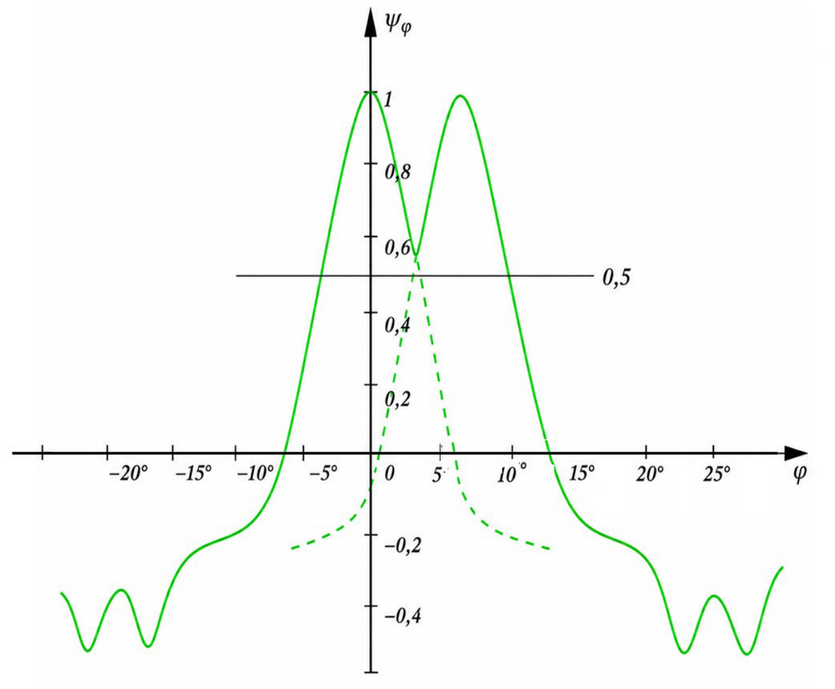
Figure 8 shows the UF of a traditional sum-of-squares integrator (red) and a Wilcoxon rank detector (green) at q² = 20 dB, calculated using equation (20); Figure 9 shows the UF of two signals separated by 12.5 degrees in angle, and Figure 10 shows the UF of two signals separated by 7.5 degrees in angle. The graphs show that, in the main lobe region of the beam pattern, the frequency response of rank-based detectors using the spatial-temporal ranking method is virtually indistinguishable from that of a traditional sum-of-squares integrator. However, in the side lobes of the beam pattern, the rank detector’s UF has a significant negative component, which is caused by the presence of an intense signal in the reference cell. Nevertheless, since the detection threshold is positive in rank-based processing, these side lobes cannot cause false alarms and, therefore, pose no danger. Figure 10 also shows that when using the Wilcoxon rank detector, signals separated by an angle of less than 7.5 degrees are no longer distinguishable.
5. Conclusions
Thus, based on the analysis of the frequency response, it can be concluded that the ranking procedure does not lead to a broadening of the main peak of the frequency response or an increase in the level of the side lobes for those signal parameters used to form the reference cell. Thus, with the temporal ranking method, good signal distinguishability is preserved over time, and with the spatial-temporal method, it is preserved both over time and in space. For those coordinates that do not participate in the formation of the reference array, the UF of the rank-based detector deteriorates significantly compared to the traditional sum-of-squares method. In this regard, combined ranking methods can be recommended, in which the reference cell is formed based on several coordinates.
Author Contributions
Conceptualization, Y.B.-B. and M.A.; methodology, Y.B.-B. and M.A.; software, O.S., K.U. and Z.K.; validation, Y.B.-B., S.M. and S.G.; formal analysis, A.N., Z.K. and S.K.; investigation, Y.B.-B., A.N., and O.S.; writing—original draft preparation, S.M. and S.K.; writing—review and editing, Y.B.-B., S.G. and T.A.; visualization, M.A., K.U. and T.A.; supervision, Y.B.-B. All authors have read and agreed to the published version of the manuscript.
Funding
This research received no external funding.
Institutional Review Board Statement
Not applicable.
Informed Consent Statement
Not applicable.
Data Availability Statement
The original contributions presented in this study are included in the article. Further inquiries can be directed to the corresponding author(s).
Acknowledgments
The team of authors of the article expresses sincere gratitude to the scientists and specialists of the chairs “Radio-electronic systems and devices”, “Information systems and telecommunications” of N. Bauman Moscow State Technical University, whose consultations and advices were taken into account when performing scientific research.
Conflicts of Interest
The authors declare no conflicts of interest.
Abbreviations
The following abbreviations are used in this manuscript:
| UF | uncertainty function |
| PB | preprocessing block |
| RB | ranking block |
| RSC | rank statistic calculator |
| F | filter |
| D | detector |
| TD | thresholding device |
| BP | beam pattern |
References
- Bakut, P.A.; Bolshakov, I.A.; Gerasimov, B.M. Questions of the statistical theory of radar. Sovetskoe Radio: Moscow, Russia, 1964; 1080 p. (In Russian).
- Berdyshev, V. P.; Garin, E. N.; Fomin, A. N; Tyapkin, V. N.; Fateev, Yu. L.; Lyutikov, I. V.; Bogdanov, A.V.; Kordyukov, R. Y. Radar systems [Electronic resource]. Textbook. Siberian Federal University: Krasnoyarsk, Russia, 2012; 400 p. (In Russian).
- Shirokov, Yu. F. Fundamentals of Radar Systems Theory: Electronic Textbook. – Samara: S. P. Korolev Samara State Aerospace University, 2012; 129 p. (In Russian).
- Shirman, Ya.D. Theoretical foundations of radar; Soviet Radio: Moscow, Russia, 1970; 560 p. (In Russian).
- Friz, S.P.; Andreev, A.V.; Rykhalsky, A.R.; Dubina, A.F. Theory and Techniques of Radar and Radio Navigation. Zhytomyr: A.A. Yevenok Publishing House, 2020; 180 p. (In Russian).
- Bogdanov, G.B. Fundamentals of Radar. Kyiv: KVIRTU Air Defense, 1978; 285 p. (In Russian).
- Sosulin, Yu. G. Theoretical Foundations of Radar and Radio Navigation. Moscow: Radio and Communications, 1992; 304 p. (In Russian).
- Sibel, A.G. Fundamentals of Radar. Moscow: Sovetskoe Radio, 1961; 386 p. (In Russian).
- Peshkov, I.V. Radar. The training manual. I.A. Bunin Yelets State University: Yelets, Russia, 2018; 44 p. (In Russian).
- Zibrov, A. A.; Vetrov, S. V. Klimov, A. I.; Yudin, V. I.; Pasternak, Y. G. Radio Engineering Systems. Textbook. Voronezh: VSTU Press, 2002; 189 p. (In Russian).
- Kuzmin, C.Z. Digital radar. KVITS Publishing House: Kiev, Ukraine, 2000; 428 p. (In Russian).
- Mahafza, B. R. Radar Systems Analysis and Design Using MATLAB / Bassem R. Mahafza. — CHAPMAN&HALL/CRC, 2000; 532 p.
- Karpov, I.G.; Gribkov, A.N. Fundamentals of Radio Electronics and Communications. Part I. Fundamentals of Optimal Radio Reception: A Textbook. Tambov: Tambov State Technical University Press, 2009; 80 p. (In Russian).
- Vasin, V.A.; Vlasov, I.B.; Egorov, Yu.;M. et al.; edited by I.B. Fedorov. Information Technology in Radio Engineering Systems: A Textbook. Moscow: Bauman Moscow State Technical University Press, 2004; 766 p. (In Russian).
- Lezin, Yu. S. Introduction to the Theory and Design of Radio Engineering Systems: A Textbook for Universities. Moscow: Radio and Communications, 1986; 280 p. (In Russian).
- Gaek, Ya.; Shidak, Z. The theory of rank criteria. Nauka Publ: Moscow, Russia,1971; 376 (In Russian).
- David, G. Ordinal Statistics. Moscow: Nauka, 1979; 336 p. (In Russian).
- Tarasenko, F.P. Nonparametric statistics. Tomsk University Press: Tomsk, Russia, 1976; 294. (In Russian).
- Vilenkin, S.Y. Statistical Analysis of Random Function Research Results. Moscow: Energiya, 1979; 320 p. (In Russian).
- Yesmagambetov B.-B.S. Determination of the Characteristics of Non-Stationary Random Processes by Non-Parametric Methods of Decision Theory. Computation 2023, Volume 11, Issue 11, 219, Basel, November 2023. https://doi.org/10.3390/computation11110219.
- Fal'kovich, S.E. Signal Parameter Estimation. Moscow: Sovetskoe Radio, 1970; 334 p. (In Russian).
- Levin, B.R. Theoretical foundations of statistical radio engineering. Radio and Communications: Moscow, Russia, 1989; 653 p. (In Russian).
- Lebedko, E.G. Mathematical Foundations of Information Transmission. St. Petersburg: St. Petersburg State University of Information Technologies, Mechanics, and Optics (ITMO), 2009;120 p. (In Russian).
- Finkelstein, M. I. Fundamentals of Radar. Moscow: Radio and Communications, 1983; 536 p. (In Russian).
- Weinstein, L. A., Zubakov, N. D. Signal Detection in the Presence of Random Noise. Moscow: Sovetskoe Radio, 1960; 446 p. (In Russian).
- Perov, A.I. Statistical Theory of Radio Engineering Systems. Moscow: Radiotekhnika, 2003; 400 p. (In Russian).
Figure 1.
Explanation of the Selection of the Allowable Resolution Parameter Deviation.
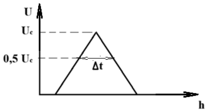
Figure 2.
Output signals of the optimal processing device.
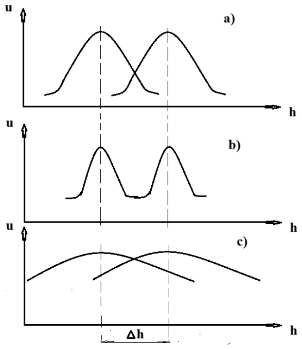
Figure 3.
Block diagram of the information ranking processing path using the temporal ranking method.
Figure 3.
Block diagram of the information ranking processing path using the temporal ranking method.
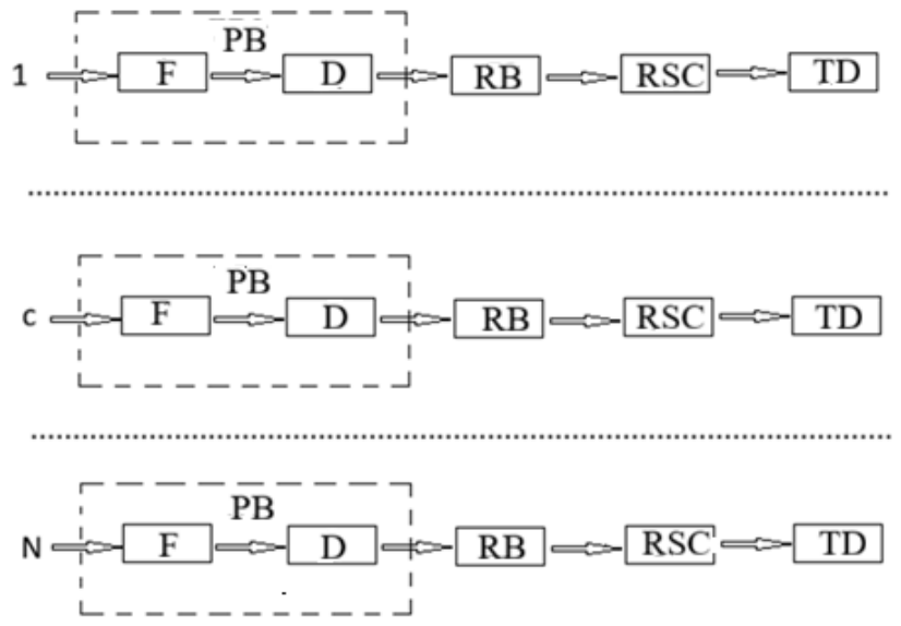
Figure 4.
Block diagram of the information ranking processing path in the spatio-temporal ranking method.
Figure 4.
Block diagram of the information ranking processing path in the spatio-temporal ranking method.
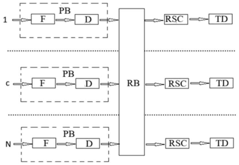
Figure 5.
Temporal uncertainty function of the traditional sum-of-squares integrator (red) and the Wilcoxon rank-sum detector (green).
Figure 5.
Temporal uncertainty function of the traditional sum-of-squares integrator (red) and the Wilcoxon rank-sum detector (green).
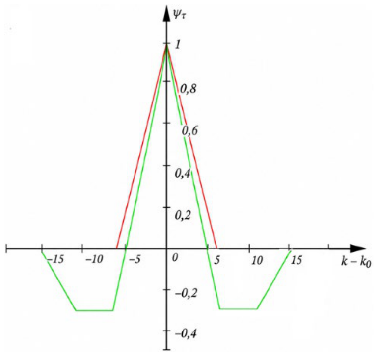
Figure 6.
Temporal uncertainty function for two signals separated by
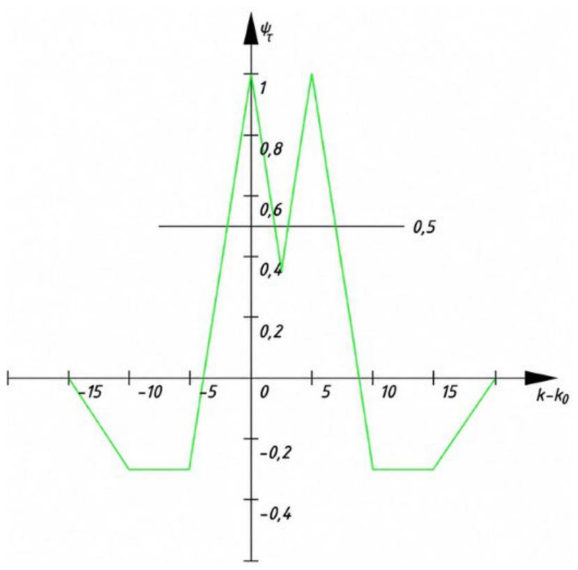
Figure 7.
Temporal uncertainty function for two signals separated by
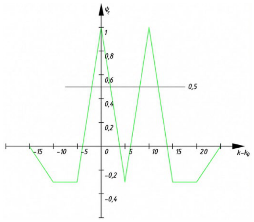
Figure 8.
Uncertainty function of the traditional sum-of-squares integrator (red) and the Wilcoxon rank-sum test (green).
Figure 8.
Uncertainty function of the traditional sum-of-squares integrator (red) and the Wilcoxon rank-sum test (green).
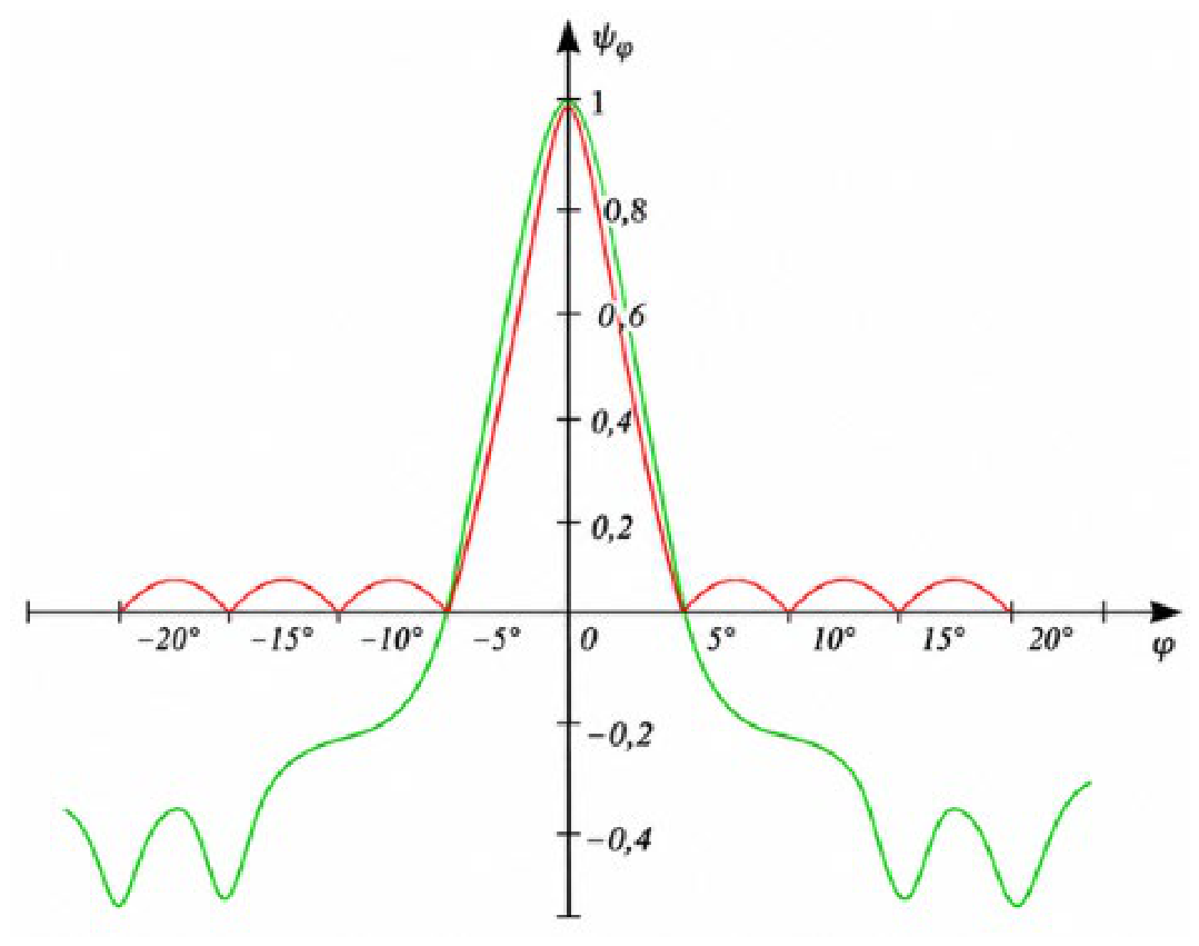
Figure 9.
Uncertainty function for two signals separated by 12.5 degrees in angle.
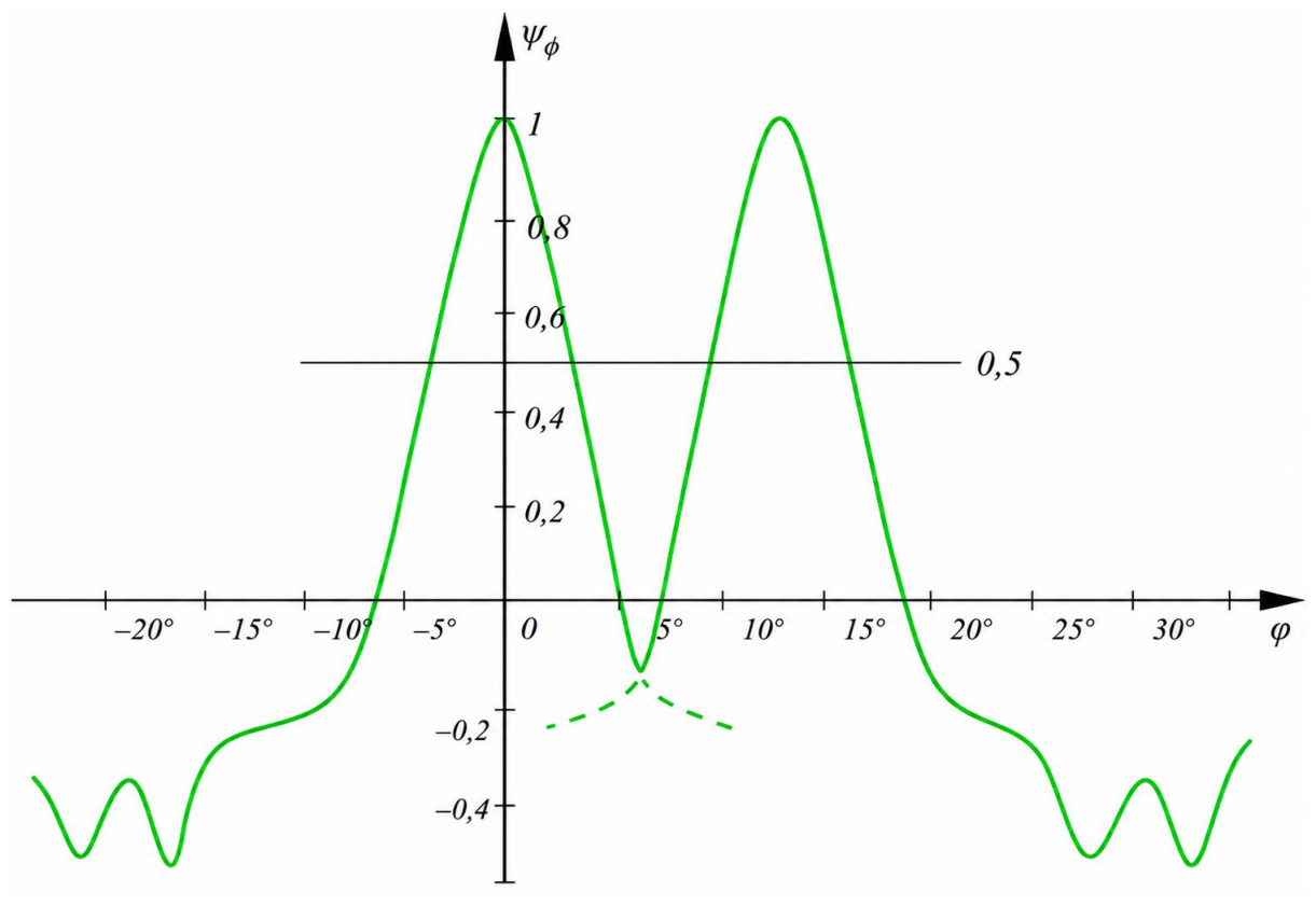
Figure 10.
Uncertainty function for two signals separated by 7.5 degrees in angle.
Disclaimer/Publisher’s Note: The statements, opinions and data contained in all publications are solely those of the individual author(s) and contributor(s) and not of MDPI and/or the editor(s). MDPI and/or the editor(s) disclaim responsibility for any injury to people or property resulting from any ideas, methods, instructions or products referred to in the content. |
© 2026 by the authors. Licensee MDPI, Basel, Switzerland. This article is an open access article distributed under the terms and conditions of the Creative Commons Attribution (CC BY) license (http://creativecommons.org/licenses/by/4.0/).
Copyright: This open access article is published under a Creative Commons CC BY 4.0 license, which permit the free download, distribution, and reuse, provided that the author and preprint are cited in any reuse.