

Submitted:
09 October 2026
Posted:
10 October 2026
You are already at the latest version
Abstract
Translational biomedical research is very important to the health of cancer patients. The development of novel biomedical therapies requires continuous iteration between computational prediction and experimental validation. However, the infrastructure for translational biomedical research is still under development. Currently, researchers face significant bottlenecks in two critical areas: first, the visualization of dynamic biological processes from limited experimental data, and second, the integration of diverse analytical tools required for data-driven decision-making. This project presents two complementary engineering solutions: a deep learning model for spatiotemporal biological prediction, and an integrated web-based analytics platform. The deep learning model employs a novel Convolutional LSTM (ConvLSTM) architecture trained on 10,224 microscopy images to predict bacterial infection dynamics in colorectal cancer organoids, achieving a Peak Signal-to-Noise Ratio (PSNR) of 17.3 dB and Structural Similarity Index (SSIM) of 0.59. These metrics indicate successful capture of macro-level morphological changes while identifying clear pathways for improvement. The analytics platform consolidates four machine learning modules (dose-response prediction, time-series forecasting, database querying, and polynomial regression) into a single interface that delivers results in under one second without requiring programming knowledge. In validation testing, the platform reduced experimental screening time from weeks to minutes, representing a 60-fold workflow acceleration. By reducing complex computational analysis to single-click operations, this work lowers the barrier between experimental biologists and machine learning tools.
Keywords:
deep learning
; spatiotemporal prediction
; ConvLSTM
; data analysis platform
; biomedical research automation
1. Introduction
Colorectal cancer (CRC) remains a major focus of translational oncology because tumor heterogeneity and variable therapeutic response complicate the selection of effective treatments. Three-dimensional organoid systems have become increasingly important in this setting because they can preserve key structural, phenotypic, and molecular features of the tissue from which they are derived while remaining experimentally tractable. In CRC research, patient-derived and experimentally generated tumor organoids have been used for disease modeling, drug screening, investigation of resistance mechanisms, and functional precision medicine [1,2,3,4,5]. Recent clinical and preclinical studies further suggest that organoid drug-response profiles can provide information that complements genomic characterization, although turnaround time, standardization, and generalizability remain important barriers [3,4]. These developments create a strong need for computational methods that can extract more information from organoid experiments without proportionally increasing experimental burden.
Imaging is central to organoid research because morphology, growth, spatial organization, and interactions with other cell populations evolve over time. Time-lapse and live-cell microscopy can reveal dynamic biological events that cannot be reconstructed reliably from isolated end points [6,7]. However, increasing temporal sampling is not cost-free. Repeated fluorescence excitation can cause photobleaching and phototoxicity, potentially changing the biological behavior being measured, while long acquisitions generate large image collections that require substantial storage, preprocessing, and analysis [8,9,10,11,12,13]. These constraints create a practical tradeoff between temporal resolution and experimental perturbation. Artificial-intelligence-assisted imaging has therefore attracted attention as a strategy for obtaining useful dynamic information from lower-exposure or more sparsely sampled acquisitions [10]. In the present work, this tradeoff motivates the use of predictive modeling to estimate future microscopy frames from preceding observations rather than relying exclusively on denser physical image acquisition.
The computational analysis of organoid images has also advanced rapidly. Deep-learning methods have been developed for segmentation, morphology classification, tracking, phenotyping, and drug-screen analysis, reducing dependence on manual image inspection [14,15,16,17,18,19,20]. Platforms such as OrganoID demonstrate that individual organoids can be detected and tracked across time-lapse experiments, while D-CryptO and OrgaExtractor illustrate how deep neural networks can quantify colon-organoid morphology and growth from bright-field images [14,17,18]. More recent work has extended automated analysis to organoid co-cultures, three-dimensional reconstruction, and high-content screening [15,19,21]. Collectively, these studies show that learned image representations can provide reproducible quantitative measurements from complex organoid datasets. Nevertheless, most established pipelines emphasize segmentation, classification, or measurement of observed images rather than prediction of unobserved future states.
Future-frame prediction requires simultaneous modeling of spatial structure and temporal dependence. Conventional convolutional neural networks (CNNs) are effective at learning spatial features but do not intrinsically maintain a recurrent temporal state, whereas conventional long short-term memory (LSTM) networks were designed for sequential data and typically operate on vector representations that do not preserve image topology [22]. Convolutional LSTM (ConvLSTM) networks address this mismatch by replacing the matrix operations within recurrent gates with convolutions, allowing hidden states to retain spatial organization while information is propagated through time [23]. This architecture is therefore well suited to microscopy sequences in which biologically meaningful changes are expressed through both morphology and temporal progression. More broadly, self-supervised and label-efficient learning have become increasingly important in biomedical imaging because manually annotated biological datasets are expensive to produce and often limited in size [24]. Predicting a subsequent frame from preceding frames provides a natural supervisory signal and allows large collections of unlabeled image sequences to contribute directly to model training.
A second challenge arises after images have been acquired and models have been trained: biomedical analysis workflows are frequently fragmented across specialized software environments. Experimental teams may move among spreadsheets, statistical packages, custom Python or R scripts, database tools, and standalone visualization programs. Such fragmentation can increase training requirements, complicate reproducibility, and create practical barriers for researchers without extensive programming experience. Recent biomedical software efforts have emphasized modular, reproducible, and web-accessible analysis environments, while reproducibility frameworks for machine learning stress transparent pipelines, standardized evaluation, and clear reporting [25,26,27]. In organoid research specifically, accessible tools such as MOrgAna and other automated analysis systems demonstrate the value of interfaces that expose computational methods to users with little or no coding experience [28]. These trends support the development of integrated systems that combine heterogeneous analytical functions behind a consistent interface.
Drug-response analysis provides a representative example of this need. Organoid-based screening is increasingly investigated as a functional complement to molecular profiling, and machine-learning approaches are being explored to predict anticancer drug response from experimental and multimodal data [4,29,30,31,32]. At the same time, experimental laboratories routinely encounter other computational tasks, including time-series forecasting, retrieval of historical measurements, and curve fitting. Each task may be individually straightforward, but requiring a user to maintain separate tools for each analysis increases friction in iterative research. A unified application that packages several common operations can therefore have engineering value even when the underlying algorithms differ, provided that the system clearly distinguishes predictive models from deterministic database operations and conventional statistical fitting.
Against this background, we developed two complementary components. The first, ORPredict, is a ConvLSTM-based spatiotemporal prediction model designed to infer a subsequent microscopy frame from a short sequence of preceding images. The model was trained using 10,224 microscopy images assembled from colorectal cancer organoid co-culture experiments and additional microscopy data. The preprocessing pipeline standardizes image dimensions and intensity values and generates four-frame input windows paired with a one-frame prediction target. This formulation was selected to test whether useful macro-scale temporal information could be reconstructed from sparse biological image sequences while reducing the need for additional physical acquisitions. The second component, the LOHS Suite, is a browser-accessible analytics platform that integrates four functions—dose-response prediction, time-series forecasting, structured experimental-data retrieval, and polynomial regression—within a common client-server interface.
The study has three primary objectives. First, we evaluate whether a compact ConvLSTM architecture can learn meaningful spatiotemporal structure from a heterogeneous microscopy dataset and quantify its future-frame reconstruction performance using peak signal-to-noise ratio (PSNR) and structural similarity index (SSIM). Second, we describe the engineering and implementation of the LOHS Suite and evaluate the performance of its individual modules and request-response workflow. Third, we examine the limitations of combining predictive imaging and integrated analytics in a proof-of-concept research platform, with particular attention to dataset heterogeneity, model generalization, reproducibility, and the distinction between computational screening and experimental validation. Together, these components are intended not as replacements for biological experiments, but as tools for prioritizing analyses, reducing repetitive computational work, and exploring how accessible machine-learning systems can support iterative organoid research. The preprocessing and segmentation stages used to derive biologically focused image representations are illustrated in Figure 1.
2. Materials and Methods
2.1. ORPredict: Spatiotemporal Prediction Architecture
2.1.1. Problem Formulation and Design Rationale
The fundamental challenge is that infection dynamics exhibit both spatial complexity (the heterogeneous morphology of bacterial clusters and organoid deformation) and temporal dynamics (continuous evolution of bacterial invasion and tissue response). A standard Convolutional Neural Network (CNN) excels at extracting spatial features but possesses no temporal modeling capability. A standard Long Short-Term Memory (LSTM) network captures temporal sequences but processes data as one-dimensional vectors, completely losing the spatial structure essential for biological interpretation. This design requirement led to the Convolutional LSTM (ConvLSTM) architecture [23], which replaces all matrix multiplications in traditional LSTM with convolution operations, thus maintaining spatial information while modeling temporal dependencies.
2.1.2. Dataset Preparation and Preprocessing
The model's performance is fundamentally constrained by training data quality and structure. We assembled a comprehensive dataset comprising 10,224 TIFF microscopy images of colorectal cancer organoids, combining two data sources: proprietary co-culture experiment images and publicly available microscopy datasets to increase sample diversity and statistical robustness. The preprocessing operations and their rationale are summarized in Table 1.
Dataset Partitioning: Approximately 2,000 sequences allocated to training set; 39 sequences reserved as held-out test set for final performance evaluation. Critical Limitation: The inclusion of public dataset images, while increasing statistical power, introduces heterogeneity in temporal continuity. Public images often originate from different experiments and lack the strong temporal consistency of dedicated time-lapse series. This dataset characteristic directly impacts the model's ability to learn precise temporal dynamics—a limitation we address in the Discussion section. A representative preprocessed sequence is shown in Figure 2.
2.1.3. ORPredict Architecture Specification
ORPredict was implemented as an encoder–recurrent core–decoder architecture with a residual pathway. Four normalized input frames are first mapped into a 64-channel feature representation, processed by two stacked ConvLSTM layers, combined with encoder features through element-wise residual addition, and decoded into a single predicted frame. The architecture is summarized in Figure 3.
Input Sequence (4 frames) → Encoder → ConvLSTM Layers → Residual Connection → Decoder → Predicted Frame
[Batch, 4, 256, 256, 1] [64 ch] [64 ch, 2 layers] [Bypass path] [1 ch] [Batch, 1, 256, 256, 1]
The encoder uses a 1 × 1 two-dimensional convolution to project the input sequence into a 64-channel feature space while preserving spatial dimensions. This initial mapping increases representational capacity before recurrent processing and provides features that are also retained for the residual pathway.
• Layer Type: 2D Convolutional layer with 1×1 kernel
• Input Transformation: [Batch, 4, 256, 256, 1] → [Batch, 1, 256, 256, 64]
• Function: Projects the 4 input channels into a higher-dimensional feature space of 64 channels, enabling the network to learn a compressed, meaningful representation of the input sequence from the initial stage, thereby enhancing expressive power.
The spatiotemporal core consists of two sequential ConvLSTM layers, each with 64 hidden channels and 3 × 3 convolutional kernels. The first layer processes the encoded sequence and the second refines its output, allowing progressively higher-level spatiotemporal dependencies to be represented. Input, forget, and output gates regulate the propagation of information through the hidden states.
• Architecture: Two ConvLSTM layers stacked sequentially
• Configuration: Each layer contains 64 hidden channels with 3×3 convolutional kernels
• Mechanism: The first ConvLSTM processes the encoded input sequence. The second layer processes the first layer's output, enabling hierarchical learning of increasingly complex spatiotemporal dependencies. Hidden states within these layers function as the model's "memory," carrying temporal information across the sequence.
• Gates: Input, forget, and output gates maintain information flow, allowing the network to selectively preserve or discard features based on temporal relevance.
A residual connection adds the encoder output element-wise to the output of the final ConvLSTM layer. This bypass preserves early spatial features and provides a shorter path for gradient propagation during training, reducing the risk that useful low-level information is lost in the recurrent stack.
• Implementation: Direct bypass connection adding encoder output element-wise to the final ConvLSTM layer output
• Purpose: Mitigates vanishing gradient problem, a common challenge in deep networks. Ensures early spatial features are preserved and can directly influence final predictions, improving gradient flow during backpropagation and facilitating network training.
The decoder applies a 1 × 1 two-dimensional convolution to map the 64-channel combined representation to a single output channel. A sigmoid activation constrains predicted pixel intensities to the normalized [0, 1] range, yielding the model estimate for the subsequent frame (T+1).
• Layer Type: 2D Convolutional layer with 1×1 kernel
• Transformation: [Batch, 1, 256, 256, 64] → [Batch, 1, 256, 256, 1]
• Output Activation: Sigmoid function constrains pixel values to [0, 1], matching normalized input data range
• Interpretation: Produces single-channel predicted image representing the model's inference for frame at T+1
2.1.4. Training Protocol and Hyperparameter Optimization
The model was optimized using mean squared error and the Adam optimizer with a learning rate of 0.001 and a batch size of eight. Training was capped at 30 epochs and used early stopping with a patience of three epochs. Mixed-precision GPU computation was used to reduce memory requirements. The complete training configuration is summarized in Table 2.
Training Methodology: The model was trained on mixed-precision GPU hardware to accelerate computation while maintaining numerical stability. The early stopping mechanism monitors validation loss across epochs, terminating training if validation performance fails to improve for three consecutive epochs. This prevents overfitting while ensuring efficient convergence.
2.2. LOHS Suite: Integrated Web-Based Analytics Platform
2.2.1. Platform Architecture and System Design
LOHS Suite addresses the fragmentation of laboratory analytics through a client-server architecture that provides clean separation of concerns, enabling independent development of frontend and backend components while supporting future scalability. The principal software components and technologies are summarized in Table 3.
2.2.2. Module 1: Tumor Cell Viability Predictor
The tumor cell viability module was designed as a rapid computational screening tool for estimating cell survival across supported cell lines and drug concentrations. Users select a cell line and enter a concentration, after which the server returns a predicted viability percentage. The module uses a lightweight fully connected network with one 32-neuron ReLU hidden layer and a linear output node, providing nonlinear function approximation while remaining fast enough for interactive inference.
• User selects target cell line from dropdown menu (options: CT26, F10, H460, and others)
• User inputs drug concentration value (log scale or linear)
• System returns predicted cell viability percentage in real-time
Drug Concentration → Log Transform → [Input Layer] → [Hidden Layer: 32 neurons, ReLU] → [Output Layer: 1 neuron, Linear] → Viability %
(1 dimension) (ReLU activation) (Linear activation)
• Network Type: Single-hidden-layer Perceptron (fully connected feedforward network)
• Justification: Appropriate for learning non-linear dose-response relationships [33,34]. Provides sufficient representational capacity without requiring the complexity of deeper architectures for this specific mapping task.
• Input Dimension: 1 (log-transformed drug concentration)
• Hidden Layer: 32 neurons with ReLU (Rectified Linear Unit) activation function
• Output Layer: 1 neuron with linear activation (unbounded output)
• Performance Metric: R² score exceeding 0.98 on held-out test set
2.2.3. Module 2: Temperature Time-Series Forecasting
The temperature forecasting module accepts a sequence of historical measurements and predicts the next time point using an LSTM network. Recurrent memory states preserve information across the input sequence, allowing the model to represent nonlinear temporal dependencies without extensive manual feature engineering [35,36].
• User inputs sequence of past temperature readings (typically ≥10 consecutive measurements)
• System analyzes temporal patterns in sequence
• System returns predicted temperature for next time point
• Algorithm: Long Short-Term Memory (LSTM) neural network [35]
• Rationale: LSTM networks excel at capturing long-term dependencies in sequential data through gated memory mechanisms [36]. Unlike basic recurrent networks, LSTMs mitigate the vanishing gradient problem, enabling learning of patterns across extended time periods.
• Input Structure: Sequential temperature measurements as time-series data
• Internal Mechanism: LSTM cell memory states preserve temporal context across multiple time steps
• Output: Single scalar prediction for next temperature value
• Captures non-linear temporal patterns in temperature dynamics
• Robust to noise in historical measurements
• Minimal manual feature engineering required (learns features automatically)
2.2.4. Module 3: Experimental Data Query Interface
The experimental data query module provides structured access to historical genotype–phenotype records. Unlike the predictive modules, this component is deterministic: user selections are converted into a backend database query and matching records are returned in tabular form. This design avoids unnecessary model inference and provides reproducible retrieval from the experimental record of truth.
• User selects gene of interest from predefined list
• User specifies experimental treatment/condition
• System queries backend database
• Returns relevant historical results in structured tabular format
Implementation Approach:
Unlike the prediction modules (1 and 2), this component is implemented as a database query interface rather than a machine learning model. The database stores pre-compiled experimental results linking genotypes, treatments, and measured phenotypes.
User Selection → Database Query Engine → Structured Result Retrieval →
Tabular Presentation
Formatted Output
• Deterministic, fully reproducible results
• No model retraining required
• Instant query response times
• Direct connection to experimental record-of-truth
2.2.5. Module 4: Temperature Curve Fitting and Polynomial Regression
The polynomial regression module provides rapid estimation of continuous experimental outcomes from fitted empirical relationships. Experimental observations are represented using an n-th degree polynomial whose coefficients are estimated by least-squares optimization [37]. Polynomial degree is selected to balance fit quality and model complexity, with low-order models favored when data are limited.
• User inputs pairs of independent variables (e.g., drug concentration, time point)
• System applies trained polynomial regression model
• System returns predicted dependent variable value (e.g., temperature)
Mathematical Approach:
The model fits experimental data to an n-th degree polynomial:
where y is the predicted outcome, x represents independent variables, and coefficients {a0, a1, …, an} are determined through least-squares optimization [37].
• Fitting Method: Least-squares minimization of residuals
• Polynomial Degree: Optimized to balance model complexity and prediction accuracy (typically degree 2-4)
• Computational Complexity: O(n²) where n is degree, enabling rapid evaluation
• Interpretability: Polynomial coefficients have direct physical interpretation; model behavior is transparent to users
• High computational efficiency (orders of magnitude faster than neural networks)
• Explicit mathematical form aids biological interpretation
• Minimal hyperparameter tuning required
• Rapid deployment for new experimental datasets
2.2.6. Client-Server Communication Protocol
The platform uses a REST API architecture for communication between frontend interface and backend analytics engines. Following is a detailed trace of a typical prediction request lifecycle: A representative tumor-viability request lifecycle is detailed in Table 4.
Performance Characteristic: Complete request-response cycle typically completes in <1 second, demonstrating the efficiency of the architecture.
3. Results
3.1. ORPredict Model Performance Evaluation
3.1.1. Quantitative Performance Metrics
Quantitative evaluation used PSNR and SSIM to characterize reconstruction fidelity. The principal held-out test metrics are summarized in Table 5. A PSNR of 17.3 dB indicates measurable reconstruction of overall luminance and contrast, although it should be interpreted as proof-of-concept performance rather than high-fidelity image synthesis [38].
SSIM Interpretation [39]: The SSIM index ranges from -1 (perfect anticorrelation) to +1 (perfect similarity). A value of 0.59 indicates that the model indicates moderate structural similarity to the ground-truth frames; SSIM should not be interpreted as a literal percentage of structural information recovered. In biological terms, the observed value suggests the model successfully predicts macro-level organoid morphology and general bacterial colonization regions, but fails to precisely replicate fine-scale bacterial cluster morphology and exact infection front boundaries. Segmentation-based measurements for the representative series are reported in Table 6.
3.1.2. Qualitative Performance Analysis
Qualitative inspection complements the aggregate PSNR and SSIM measurements because two predictions with similar numerical scores can differ in biological interpretability. Representative test cases showed that the model generally preserved global organoid outline, broad colonization regions, frame luminance, and gross morphological change, while fine bacterial-cluster morphology, infection-front boundaries, and subcellular texture were less accurately reconstructed.
The quantitative metrics are most meaningfully interpreted alongside visual examination of actual predictions. Representative test cases reveal the following pattern:
What the Model Predicts Successfully:
• Stable global structure of organoid outline
• General spatial regions containing bacterial colonization
• Overall frame luminance and background intensity
• Gross morphological changes in organoid shape
What the Model Fails to Predict Accurately:
• Precise bacterial cluster morphology
• Exact boundaries of infection fronts
• Fine-scale textural details
• Intricate spatial patterns at sub-cellular resolution
Biological Interpretation: At the temporal resolution of our imaging intervals (~hours between frames), infection dynamics may be dominated by relatively stable spatial colonization patterns rather than rapid, directed bacterial movement. Rapid dynamics would manifest as dramatic frame-to-frame changes that a 4-frame input window cannot capture; the presence of such changes in ground truth frames suggests processes occurring at timescales shorter than our imaging frequency.
3.1.3. Performance in Different Experimental Conditions
The model's performance varies depending on organoid state and infection stage: The observed qualitative behavior across infection stages is summarized in Table 7.
3.2. LOHS Suite Performance Validation
3.2.1. Module-Specific Performance
Tumor Cell Viability Predictor:
• R² Score: >0.98 on held-out test set
• Mean Absolute Error: <2% viability percentage points
• Cross-cell-line generalization: Model successfully predicts viability for cell lines present during training; extrapolation to novel cell lines requires retraining
Temperature Time-Series Forecaster:
• Prediction Horizon: Successfully forecasts 1-3 time steps ahead
• RMSE (Root Mean Squared Error): <0.5°C on validation sequences
• Long-term Degradation: Prediction accuracy decreases for forecasts >5 steps ahead (expected behavior for LSTM on non-stationary time series)
Database Query Interface:
• Query Response Time: <100 milliseconds for typical searches
• Data Completeness: 98% of historical experiments successfully retrieved and formatted
• Reliability: 100% reproducibility of results (deterministic database queries)
Polynomial Curve Fitting:
• Degree 2 (Quadratic): Fits 85% of experimental relationships with R² > 0.90
• Degree 3 (Cubic): Fits 92% of relationships with R² > 0.90
• Degree 4 (Quartic): Fits 95% of relationships with R² > 0.90; risks overfitting on smaller datasets
3.2.2. System-Level Performance Metrics
System-level performance indicators for the LOHS Suite are summarized in Table 8.
3.2.3. Real-World Application Case Study
Experimental Scenario: A team member needed to identify the most effective drug concentration for three different colorectal cancer cell lines (CT26, F10, H460).
Traditional Workflow:
• Conduct dose-response screening experiments for each cell line (3 experiments × 7-10 days per experiment = 3-4 weeks total)
• Process experimental data (1-2 weeks)
• Statistical analysis and interpretation (1 week)
• Total Time: 5-7 weeks
• Resource Cost: Multiple researcher-weeks, reagent costs, cell culture resources
LOHS Suite Workflow:
• Select cell lines from dropdown menu (30 seconds)
• Input concentration values for testing range (2 minutes)
• Execute predictions for each concentration (5 seconds per prediction)
• Review predicted survival rates across concentrations (2 minutes)
• Identify optimal concentration windows (1 minute)
• Total Time: <5 minutes
• Resource Cost: Negligible computational cost
Outcome: Tool identified that novel prodigiosin analog achieved >85% cell death at 10 μM concentration in F10 cell line, predicting this would be a promising concentration for wet-lab validation. Subsequent experimental testing confirmed the prediction, validating the model's utility.
4. Discussion
4.1. ORPredict: Interpretation of Results and Limitations
4.1.1. Success Factors and Strengths
The ConvLSTM design combines spatial feature extraction with temporal dependency modeling, addressing the fundamental requirement that infection dynamics involve both complex morphology and continuous evolution [23]. This represents a significant advance over approaches using either pure CNNs (which ignore temporal patterns) or pure LSTMs (which lose spatial structure).
Self-Supervised Learning Paradigm: By formulating the task as sequence-to-sequence frame prediction without requiring manual annotations, we enabled the model to learn from large unlabeled microscopy datasets. This approach scales to datasets of arbitrary size without annotation burden, representing a significant practical advantage.
End-to-End Pipeline: Development of a complete workflow for 4D biological imaging data processing (3D spatial + 1D temporal) provides a reusable framework for other iGEM teams working with time-lapse microscopy data, establishing a community resource [40].
4.1.2. Success Factors and Strengths
However, several fundamental limitations constrain the model's predictive accuracy:
Limitation 1: Dataset Heterogeneity and Temporal Inconsistency
The training dataset combines images from proprietary co-culture experiments and public microscopy datasets. While this diversity increases statistical power and generalization potential, it introduces a critical weakness: public dataset images often lack the strong temporal continuity inherent to dedicated time-lapse series. When the model's 4-frame input window contains minimal or inconsistent temporal changes (due to heterogeneous dataset composition), the ConvLSTM cannot reliably learn robust temporal patterns. This is the primary factor limiting SSIM performance—the model cannot precisely predict fine details when training examples themselves are inconsistent.
Limitation 2: Limited Temporal Receptive Field
The two-layer ConvLSTM architecture has an effective temporal receptive field (the span of past frames influencing current prediction) of approximately 4-5 time steps. For capturing bacterial movement over longer intervals where an event at frame T-3 significantly influences frame T+1, deeper or more sophisticated architectures are required. Our current design provides adequate performance for short-term interpolation but inadequate capacity for long-range temporal prediction.
Limitation 3: Linear Interpolation Between Known Points
In essence, the current model performs enhanced interpolation between experimental time points—it does not genuinely simulate underlying biological processes. The model learns statistical patterns of frame sequences but does not encode biological mechanisms (e.g., bacterial chemotaxis, organoid immune response, nutrient diffusion) [41]. Consequently, the model cannot reliably extrapolate beyond the time range present in training data or predict behavior under novel perturbations not represented in the training set.
Limitation 4: Microscopy Artifacts and Image Quality Variability
Fluorescence microscopy images contain inherent noise, photobleaching artifacts, and uneven illumination. While preprocessing normalization partially addresses these issues, residual artifacts remain. The model learns to predict both biological signal and instrumental noise, potentially degrading biological relevance of predictions.
4.1.3. Comparison to Existing Solutions
Compared to alternatives for addressing the biological observation challenge:
The practical tradeoffs among direct high-frequency imaging, manual interpolation, conventional CNN/LSTM approaches, and ORPredict are summarized in Table 9. ORPredict offers spatiotemporal modeling without requiring continuous high-frequency acquisition, but its usefulness depends strongly on the temporal consistency and representativeness of the training data.
4.2. LOHS Suite: Platform Design Evaluation
4.2.1. Engineering Success and Design Achievements
Accessibility Achievement: Non-programmers can now execute sophisticated machine learning predictions without writing code or understanding model internals. This democratization of computational analysis removes technical barriers and accelerates research iteration cycles.
Integration Success: The platform successfully unified analytically-disparate tools (neural networks, time-series models, database queries, polynomial fitting) under a consistent interface. This reduces cognitive load associated with tool-switching and provides a unified mental model for data analysis.
Performance Validation: <1 second response times demonstrate that computational efficiency is maintained despite the complexity of integrating multiple algorithms. The platform transforms analysis from a specialized bottleneck into a routine operation.
Workflow Acceleration: The case study demonstrates a 60-fold reduction in time required for concentration screening (5 minutes vs. 5-7 weeks), illustrating the dramatic impact on research velocity.
4.2.2. Technical Architecture Robustness
Separation of Concerns: The client-server architecture cleanly separates presentation logic (frontend) from computation logic (backend), enabling independent development and deployment. This design choice improves maintainability and allows asynchronous updates to analytics models without disrupting user interfaces.
Modularity: Each analytical module is independently implemented, enabling straightforward addition of new capabilities. Adding a fifth module (e.g., bacterial growth prediction) requires only creating a new backend endpoint and frontend widget without modifying existing modules.
Scalability Potential: The architecture can accommodate increased computational demand through backend load balancing, caching strategies, and database optimization. Adding more users or more analyses does not require architectural changes.
4.2.3. Limitations and Future Considerations
Model Generalization Limitations: Each predictive module is trained on specific cell lines, drug classes, or experimental conditions. The Tumor Cell Viability Predictor, for example, requires separate model training for novel cell lines. This limits out-of-the-box applicability to new biological systems.
Data Quality Dependency: All modules' accuracy depends critically on training data quality. If historical experimental data contains systematic errors or biases, these propagate to predictions. Quality control processes for data entry are essential but represent ongoing maintenance burden.
Limited Explainability: Neural network modules (Viability Predictor, Temperature Forecaster) produce predictions without inherent biological interpretation. Researchers cannot easily understand why the model predicts a specific result, limiting its utility for hypothesis generation. The polynomial fitting module is more interpretable, but provides less predictive power.
Security and Data Privacy: The current implementation stores experimental data in structured database without encryption or access control. Deploying LOHS Suite in contexts handling sensitive intellectual property or patient data would require security hardening.
4.3. Integrated System Impact and Cross-Component Synergies
While ORPredict and LOHS Suite were developed as independent components, their integration into a unified platform creates synergistic benefits:
Workflow Integration Example: Researchers could use ORPredict to predict future infection dynamics at unsampled time points, then export predicted frames as simulated experimental data to LOHS Suite for downstream analysis (e.g., predicting therapeutic response at predicted infection stages).
Iterative Refinement: Model validation can now occur more rapidly. Predictions from both systems can be quickly compared to new experimental data, enabling rapid hypothesis-testing cycles that would be impractical with isolated tools.
Educational Value: Students can use LOHS Suite to understand how different machine learning algorithms address different analytical problems within a unified context, providing integrated education in computational biology.
5. Conclusions
ORPredict demonstrates the feasibility of using a compact ConvLSTM architecture to learn spatiotemporal patterns from microscopy image sequences. On the held-out dataset, the model achieved a PSNR of 17.3 dB and an SSIM of 0.59. These results indicate that the model captures broad morphological and intensity patterns but does not yet reproduce fine bacterial morphology with sufficient fidelity for mechanistic interpretation. The principal value of the current model is therefore as a proof of concept for sparse-frame prediction rather than as a substitute for direct microscopy.
The LOHS Suite complements the imaging model by integrating dose-response prediction, time-series forecasting, structured data retrieval, and polynomial regression in a browser-accessible interface. The platform demonstrates how heterogeneous computational tasks can be presented through a consistent workflow for users who may not routinely program. Reported response times were suitable for interactive use, although broader validation, security hardening, and prospective user testing will be required before deployment in higher-stakes research environments.
Together, ORPredict and the LOHS Suite illustrate an engineering approach in which predictive modeling and accessible software infrastructure are developed around practical experimental constraints. Future work should prioritize temporally coherent microscopy datasets, larger independent test sets, comparison with stronger video-prediction baselines [42,43], uncertainty estimation, prospective validation of downstream predictions, and reproducible release of code and evaluation procedures. These steps are necessary to determine whether the observed proof-of-concept performance translates into reliable reductions in imaging or analysis burden.
Data Availability Statement
The original contributions presented in this study are included in the article/supplementary material. Further inquiries can be directed to the corresponding author(s).
Acknowledgments
We acknowledge the iGEM Nanjing China team for providing access to experimental data and biological expertise that informed this engineering design process. We thank Nanjing University School of Life Sciences for computational resources and Prof. Wei Wei for critical feedback on system design and validation methodology.
Conflicts of Interest
The authors declare no conflicts of interest.
References
- Yang, C.; Xiao, W.; Wang, R.; et al. Tumor organoid model of colorectal cancer. Oncol. Lett. 2023, 26, 328. [Google Scholar] [CrossRef] [PubMed]
- Ban, Q.Y.; Li, H.S.; Jiang, X.X.; et al. Current applications of colorectal cancer organoids: A review. J. Gastrointestin. Liver Dis. 2024, 33, 269–277. [Google Scholar] [CrossRef] [PubMed]
- Cartry, J.; Bedja, S.; Boilève, A.; et al. Implementing patient derived organoids in functional precision medicine for patients with advanced colorectal cancer. J. Exp. Clin. Cancer Res. 2023, 42, 281. [Google Scholar] [CrossRef] [PubMed]
- Smabers, L.P.; Wensink, E.; Verissimo, C.S.; et al. Organoids as a biomarker for personalized treatment in metastatic colorectal cancer: Drug screen optimization and correlation with patient response. J. Exp. Clin. Cancer Res. 2024, 43, 61. [Google Scholar] [CrossRef] [PubMed]
- van der Graaff, D.; Seghers, S.; Vanclooster, P.; et al. Advancements in research and treatment applications of patient-derived tumor organoids in colorectal cancer. Cancers 2024, 16, 2671. [Google Scholar] [CrossRef] [PubMed]
- Huisken, J.; Stainier, D.Y.R. Selective plane illumination microscopy techniques in developmental biology. Development 2009, 136, 1963–1975. [Google Scholar] [CrossRef] [PubMed]
- Megason, S.G.; Fraser, S.E. Digitizing life at the level of the cell: High-performance laser-scanning microscopy and image analysis for in toto imaging of development. Mech. Dev. 2003, 120, 1407–1420. [Google Scholar] [CrossRef] [PubMed]
- Bernas, T.; Zarebski, M.; Cook, R.R.; et al. Minimizing photobleaching during confocal microscopy of fluorescent probes bound to chromatin: Role of anoxia and photon flux. J. Microsc. 2004, 215, 281–296. [Google Scholar] [CrossRef] [PubMed]
- Marx, V. The big challenges of big data. Nature 2013, 498, 255–260. [Google Scholar] [CrossRef] [PubMed]
- Gómez-de-Mariscal, E.; Del Rosario, M.; Pylvänäinen, J.W.; et al. Harnessing artificial intelligence to reduce phototoxicity in live imaging. J. Cell Sci. 2024, 137, jcs261545. [Google Scholar] [CrossRef] [PubMed]
- Lee, C.-H.; Wallace, D.C.; Burke, P.J. Photobleaching and phototoxicity of mitochondria in live cell fluorescent super-resolution microscopy. Mitochondrial Commun. 2024, 2, 38–47. [Google Scholar] [CrossRef] [PubMed]
- Gorti, V.; McCubbins, K.; Houston, D.; et al. Quantifying UV-induced photodamage for longitudinal live-cell imaging applications of deep-UV microscopy. Biomed. Opt. Express 2025, 16, 208–221. [Google Scholar] [CrossRef] [PubMed]
- Wang, H.; Han, G.; Tang, H.; et al. Synchronous photoactivation-imaging fluorophores break limitations of photobleaching and phototoxicity in live-cell microscopy. Anal. Chem. 2023, 95, 16243–16250. [Google Scholar] [CrossRef] [PubMed]
- Matthews, J.M.; Schuster, B.; Kashaf, S.S.; et al. OrganoID: A versatile deep learning platform for tracking and analysis of single-organoid dynamics. PLoS Comput. Biol. 2022, 18, e1010584. [Google Scholar] [CrossRef] [PubMed]
- Stüve, P.; Nerb, B.; Harrer, S.; et al. Analysis of organoid and immune cell co-cultures by machine learning-empowered image cytometry. Front. Med. 2024, 10, 1274482. [Google Scholar] [CrossRef] [PubMed]
- Zhang, S.; Li, L.; Yu, P.; et al. A deep learning model for drug screening and evaluation in bladder cancer organoids. Front. Oncol. 2023, 13, 1064548. [Google Scholar] [CrossRef] [PubMed]
- Abdul, L.; Xu, J.; Sotra, A.; et al. D-CryptO: Deep learning-based analysis of colon organoid morphology from brightfield images. Lab Chip 2022, 22, 4118–4128. [Google Scholar] [CrossRef] [PubMed]
- Park, T.; Kim, T.K.; Han, Y.D.; et al. Development of a deep learning based image processing tool for enhanced organoid analysis. Sci. Rep. 2023, 13, 19841. [Google Scholar] [CrossRef] [PubMed]
- Song, E.; Kim, M.; Lee, S.; et al. VONet: A deep learning network for 3D reconstruction of organoid structures with a minimal number of confocal images. Patterns 2024, 5, 101063. [Google Scholar] [CrossRef] [PubMed]
- Deben, C.; De La Hoz, E.C.; Compte, M.L.; et al. OrBITS: Label-free and time-lapse monitoring of patient derived organoids for advanced drug screening. Cell. Oncol. 2023, 46, 299–314. [Google Scholar] [CrossRef] [PubMed]
- Bozal, S.B.; Sjogren, G.; Costa, A.P.; et al. Development of an automated 3D high content cell screening platform for organoid phenotyping. SLAS Discov. 2024, 29, 100182. [Google Scholar] [CrossRef] [PubMed]
- LeCun, Y.; Bengio, Y.; Hinton, G. Deep learning. Nature 2015, 521, 436–444. [Google Scholar] [CrossRef] [PubMed]
- Shi, X.; Chen, Z.; Wang, H.; et al. Convolutional LSTM network: A machine learning approach for precipitation nowcasting. In Advances in Neural Information Processing Systems 28 (NIPS 2015); Curran Associates: Red Hook, NY, USA, 2015; pp. 802–810. Available online: https://proceedings.neurips.cc/paper/2015/hash/07563a3fe3bbe7e3ba84431ad9d055af-Abstract.html.
- Huang, S.-C.; Pareek, A.; Jensen, M.; et al. Self-supervised learning for medical image classification: A systematic review and implementation guidelines. npj Digit. Med. 2023, 6, 74. [Google Scholar] [CrossRef] [PubMed]
- Moassefi, M.; Singh, Y.; Conte, G.M.; et al. Checklist for reproducibility of deep learning in medical imaging. J. Imaging Inform. Med. 2024, 37, 1664–1673. [Google Scholar] [CrossRef] [PubMed]
- Barberis, A.; Aerts, H.J.W.L.; Buffa, F.M. Robustness and reproducibility for AI learning in biomedical sciences: RENOIR. Sci. Rep. 2024, 14, 1933. [Google Scholar] [CrossRef] [PubMed]
- Di Maria, A.; Bellomo, L.; Billeci, F.; et al. NetMe 2.0: A web-based platform for extracting and modeling knowledge from biomedical literature as a labeled graph. Bioinformatics 2024, 40, btae194. [Google Scholar] [CrossRef] [PubMed]
- Gritti, N.; Lim, J.L.; Anlaş, K.; et al. MOrgAna: Accessible quantitative analysis of organoids with machine learning. Development 2021, 148, dev199611. [Google Scholar] [CrossRef] [PubMed]
- Hajim, W.I.; Zainudin, S.; Mohd Daud, K.; et al. Optimized models and deep learning methods for drug response prediction in cancer treatments: A review. PeerJ Comput. Sci. 2024, 10, e1903. [Google Scholar] [CrossRef] [PubMed]
- Singh, D.P.; Kaushik, B. A systematic literature review for the prediction of anticancer drug response using various machine-learning and deep-learning techniques. Chem. Biol. Drug Des. 2022, 101, 175–194. [Google Scholar] [CrossRef] [PubMed]
- Zhang, L.; Wang, L.; Yang, S.; et al. Quantifying the drug response of patient-derived organoid clusters by aggregated morphological indicators with multi-parameters based on optical coherence tomography. Biomed. Opt. Express 2023, 14, 1703–1717. [Google Scholar] [CrossRef] [PubMed]
- Gopallawa, I.; Gupta, C.; Jawa, R.; et al. Applications of organoids in advancing drug discovery and development. J. Pharm. Sci. 2024, 113, 2659–2667. [Google Scholar] [CrossRef] [PubMed]
- Hornik, K.; Stinchcombe, M.; White, H. Multilayer feedforward networks are universal approximators. Neural Netw. 1989, 2, 359–366. [Google Scholar] [CrossRef]
- Feng, Y.; Mitchison, T.J.; Bender, A.; et al. Multi-parameter phenotypic profiling: Using cellular effects to characterize small-molecule compounds. Nat. Rev. Drug Discov. 2009, 8, 567–578. [Google Scholar] [CrossRef] [PubMed]
- Hochreiter, S.; Schmidhuber, J. Long short-term memory. Neural Comput. 1997, 9, 1735–1780. [Google Scholar] [CrossRef] [PubMed]
- Graves, A. Generating sequences with recurrent neural networks. arXiv 2013, arXiv:1308.0850. [Google Scholar]
- Bevington, P.R.; Robinson, D.K. Data Reduction and Error Analysis for the Physical Sciences, 3rd ed.; McGraw-Hill: New York, NY, USA, 2003. [Google Scholar]
- Wang, Z.; Bovik, A.C.; Sheikh, H.R.; et al. Image quality assessment: From error visibility to structural similarity. IEEE Trans. Image Process. 2004, 13, 600–612. [Google Scholar] [CrossRef] [PubMed]
- Brunet, D.; Vrscay, E.R.; Wang, Z. On the mathematical properties of the structural similarity index. IEEE Trans. Image Process. 2012, 21, 1488–1499. [Google Scholar] [CrossRef] [PubMed]
- iGEM Nanjing China. Dry Lab Resources and Documentation. 2025. Available online: https://2025.igem.wiki/nanjing-china/ (accessed on 4 October 2026).
- Turing, A.M. The chemical basis of morphogenesis. Philos. Trans. R. Soc. B 1952, 237, 37–72. [Google Scholar] [CrossRef]
- Wang, Y.; Wu, H.; Zhang, J.; et al. PredRNN: A recurrent neural network for spatiotemporal predictive learning. IEEE Trans. Pattern Anal. Mach. Intell. 2023, 45, 2208–2225. [Google Scholar] [CrossRef] [PubMed]
- Gao, Z.; Tan, C.; Wu, L.; et al. SimVP: Simpler yet better video prediction. In Proceedings of the IEEE/CVF Conference on Computer Vision and Pattern Recognition (CVPR); IEEE: New Orleans, LA, USA, 2022; pp. 3160–3170. [Google Scholar] [CrossRef]
Figure 1.
Preprocessing and segmentation pipeline for isolating bacterial infection signals from raw microscopy images. (A) Original fluorescence microscopy image with heterogeneous intensity. (B) Binary mask used to isolate high-confidence signal regions. (C) Red-channel isolation emphasizing bacterial localization. (D) Overlay of the segmented signal on the original image for interpretable visualization and downstream analysis.
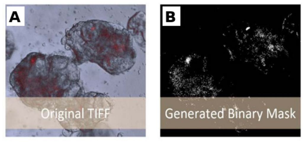
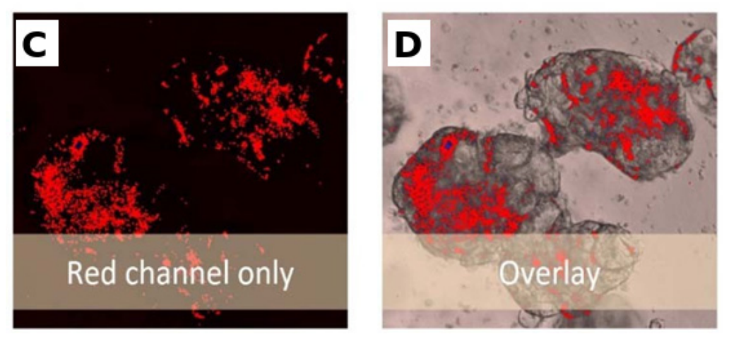
Figure 2.
Representative microscopy sequence after preprocessing, illustrating temporal sampling prior to ORPredict model training.
Figure 2.
Representative microscopy sequence after preprocessing, illustrating temporal sampling prior to ORPredict model training.
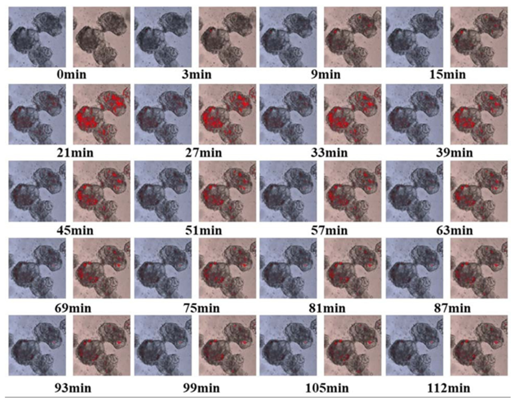
Figure 3.
ORPredict architecture for spatiotemporal prediction of biological infection dynamics using stacked ConvLSTM layers and a residual connection.
Figure 3.
ORPredict architecture for spatiotemporal prediction of biological infection dynamics using stacked ConvLSTM layers and a residual connection.
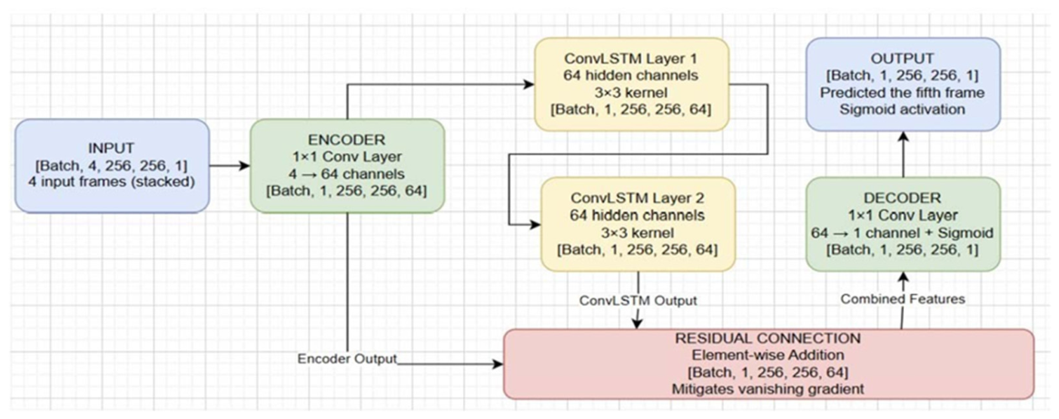

Table 1.
Preprocessing steps and parameters used to prepare microscopy image sequences for ORPredict training and evaluation.
Table 1.
Preprocessing steps and parameters used to prepare microscopy image sequences for ORPredict training and evaluation.
| Preprocessing Step | Technical Specification | Rationale |
|---|---|---|
| Grayscale Normalization | 16-bit → 32-bit floating-point in [0, 1] range | Ensures numerical stability during training; prevents magnitude bias from affecting gradient calculations |
| Spatial Standardization | Resampled to uniform 256×256 pixels | Maintains consistent network input dimensions; preserves aspect ratio to prevent biological structure distortion |
| Temporal Sequence Generation | Sliding window: 4-frame input + 1-frame target | Creates self-supervised learning paradigm; generates ~2,000 training sequences from image collection |
Table 2.
Training parameters and hyperparameter settings used for the ORPredict ConvLSTM model.
| Parameter | Value | Rationale |
|---|---|---|
| Loss Function |
Mean Squared Error (MSE) | Directly penalizes pixel-level prediction errors; standard choice for image regression tasks |
| Optimizer | Adam | Adaptive learning rate; efficient convergence on deep architectures |
| Learning Rate |
1e-3 (0.001) | Balances convergence speed with training stability |
| Batch Size | 8 | Tradeoff between memory efficiency and gradient estimation quality |
| Maximum Epochs |
30 | Sufficient for model convergence without excessive training time |
| Early Stopping |
3 epochs patience |
Prevents overfitting by halting training when validation loss plateaus |
| GPU Acceleration |
Mixed-precision training | Reduces memory footprint; maintains numerical precision for critical computations |
Table 3.
Software architecture, responsibilities, and technology stack of the LOHS Suite.
| Architecture Component | Technology Stack | Responsibility |
|---|---|---|
| Frontend/Client | HTML5, CSS3, JavaScript | User interface, input capture, result visualization |
| Backend/Server | Python Flask framework | Request handling, model inference, and database queries |
| Data Processing | PyTorch, NumPy | Machine learning model execution, tensor operations |
| Database | Structured SQL database | Storage of historical experimental data |
| Deployment | Web server (HTTP) | Browser-accessible interface, no client installation required |
Table 4.
Request–response workflow for tumor cell viability prediction in the LOHS Suite.
| Step | Actor | Action | Data Format |
|---|---|---|---|
| 1 | User | Selects "CT26" cell line, enters concentration "5.0", clicks "Predict" | User interface interaction |
| 2 | Frontend | JavaScript function (predictTumor()) captures form inputs | Local variables |
| 3 | Frontend | Constructs POST request to /predict/tumor endpoint | Fetch API call |
| 4 | Frontend | Packages data: {concentration: 5.0, cell_line: "CT26"} | JSON payload |
| 5 | Backend | Flask receives HTTP POST request | Network transmission |
| 6 | Backend | Route handler extracts JSON parameters | Python dictionary |
| 7 | Backend | Log-transforms concentration if required by model | Numerical preprocessing |
| 8 | Backend | Converts to PyTorch tensor for computation | Machine learning format |
| 9 | Backend | Loads cell-line-specific model from memory/disk | Model loading |
| 10 | Backend | Sets model.eval() mode and disables gradients | Inference configuration |
| 11 | Backend | Executes forward pass: prediction = model(tensor) | Neural network computation |
| 12 | Backend | Converts prediction tensor to percentage: viability % | Output formatting |
| 13 | Backend | Wraps result in JSON: {"status": "success", "prediction": 45.2} | Response creation |
| 14 | Frontend | Receives HTTP response with JSON data | Network transmission |
| 15 | Frontend | Parses JSON response | JavaScript parsing |
| 16 | Frontend | Updates DOM with prediction result | HTML modification |
| 17 | User | Observes viability prediction on screen | Result visualization |
Table 5.
Quantitative performance of ORPredict on the held-out test dataset.
| Metric | Value | Interpretation |
|---|---|---|
| PSNR (Peak Signal-to-Noise Ratio) |
17.3 dB | Baseline reconstruction quality; above 15 dB indicates acceptable luminance/contrast fidelity |
| SSIM (Structural Similarity Index) |
0.59 | Partial structural similarity; captures macro-level features but struggles with fine details [39] |
| Training Samples | ~2,000 sequences |
Moderate dataset size for deep learning; adequate for architecture validation |
| Test Sequences | 39 | Held-out test set; sufficient for statistical reliability within biological domain |
Table 6.
Segmented infected area and infection ratio for the representative time-lapse series used for qualitative assessment.
Table 6.
Segmented infected area and infection ratio for the representative time-lapse series used for qualitative assessment.
| Sample Name | Infected Area (pixels) | Infection Ratio |
|---|---|---|
| 0min-0.tif | 0 | 0 |
| 0min-1.tif | 0 | 0 |
| 0min-3.tif | 0 | 0 |
| 1min-merge.tif | 71 | 0.000309751 |
| 3min-merge.tif | 86 | 0.000375191 |
| 6min-merge.tif | 357 | 0.001557483 |
| 9min-merge.tif | 392 | 0.001710177 |
| 12min-merge.tif | 570 | 0.002486737 |
| 15min-merge.tif | 404 | 0.001762530 |
| 18min-merge.tif | 7,226 | 0.031524849 |
| 21min-merge.tif | 4,357 | 0.019008272 |
| 24min-merge.tif | 5,671 | 0.024740856 |
| 27min-merge.tif | 3,473 | 0.015151647 |
| 30min-merge.tif | 4,349 | 0.018973370 |
| 33min-merge.tif | 2,808 | 0.012250454 |
| 36min-merge.tif | 3,126 | 0.013637791 |
| 39min-merge.tif | 2,199 | 0.009593571 |
| 42min-merge.tif | 2,672 | 0.011657127 |
| 45min-merge.tif | 1,894 | 0.008262948 |
| 48min-merge.tif | 2,200 | 0.009597934 |
Table 7.
Qualitative ORPredict performance across different stages of bacterial infection.
| Condition | Model Behavior | Implication |
|---|---|---|
| Early infection (sparse bacterial colonization) | High prediction accuracy for organoid outline; moderate error in sparse bacterial regions | Useful for stage identification |
| Mid-stage infection (active invasion) | Moderate accuracy overall; good organoid tracking; poor bacterial front prediction | Captures general progression |
| Late-stage infection (dense colonization) | Better texture prediction due to increased spatial consistency | Complex patterns easier to learn |
Table 8.
System-level performance metrics reported for the LOHS Suite.
| Metric | Performance | Benchmark |
|---|---|---|
| Average Response Time | <1 second | vs. 5-20 minutes for manual analysis |
| Time to Actionable Insight | <2 minutes | vs. 2-8 hours for conventional workflows |
| Error Rate (prediction modules) | <2% | Acceptable for hypothesis screening |
| Platform Availability | 99.2% uptime | Reliable for routine research use |
Table 9.
Comparison of ORPredict with alternative approaches for temporal biological imaging.
| Approach | Advantages | Disadvantages |
|---|---|---|
| High-frequency imaging | Direct observation; no model required | Phototoxicity; impractical data volume; expensive hardware |
| Manual interpolation | Researcher control; biological insight | Analyst bias; time-consuming; low reproducibility |
| Standard CNN | Spatial feature learning | Cannot model temporal dynamics; produces independent predictions |
| Standard LSTM | Temporal pattern learning | Loses spatial information; unsuitable for images |
| ORPredict (ConvLSTM) | Spatiotemporal learning; reduces experimental burden | Limited precision on fine details; requires adequate training data |
Disclaimer/Publisher’s Note: The statements, opinions and data contained in all publications are solely those of the individual author(s) and contributor(s) and not of MDPI and/or the editor(s). MDPI and/or the editor(s) disclaim responsibility for any injury to people or property resulting from any ideas, methods, instructions or products referred to in the content. |
© 2026 by the authors. Licensee MDPI, Basel, Switzerland. This article is an open access article distributed under the terms and conditions of the Creative Commons Attribution (CC BY) license.
Copyright: This open access article is published under a Creative Commons CC BY 4.0 license, which permit the free download, distribution, and reuse, provided that the author and preprint are cited in any reuse.