

Submitted:
09 October 2026
Posted:
10 October 2026
You are already at the latest version
Abstract
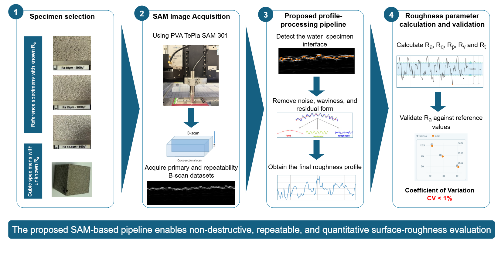
Although additive manufacturing enables the production of metallic components with complex geometries, accurately characterizing their surfaces remains challenging, especially in regions beyond the reach of conventional techniques. To address this challenge, this study investigates scanning acoustic microscopy (SAM) as an automated, non-destructive method for measuring the surface roughness of stainless steel 316L cubes fabricated by selective laser melting. A dedicated image-processing pipeline was developed to detect the water–specimen interface in SAM B-scan images and convert it into a calibrated surface profile. ISO-based spatial filtering was then applied to separate roughness from measurement noise, waviness, and surface form. The resulting profiles were used to calculate Ra, Rq, Rp, Rv, and Rt. Ra was used as the common parameter for quantitative validation of SAM against reference standards. For nominal values of 12.5, 25, and 50 μm, SAM measured 12.92, 28.53, and 51.60 μm, corresponding to absolute deviations of 0.42, 3.53, and 1.60 μm, respectively. The repeatability assessment showed coefficients of variation below 1%, indicating precise measurements. Following this assessment, the proposed pipeline was applied to the fabricated cubes and compared with digital light and laser confocal microscopes. Overall, the findings show that SAM can distinguish different roughness levels and provide reliable quantitative measurements.
Keywords:
additive manufacturing
; scanning acoustic microscopy (SAM)
; surface roughness
; non-destructive testing
; image processing
1. Introduction
Producing additively manufactured metal components that meet their functional requirements involves not only achieving the required geometry, but also obtaining a surface condition suitable for the intended application. Effectively controlling and monitoring this condition requires a clear understanding of how printing and post-processing parameters influence the final surface quality. Among the characteristics that define this quality, surface roughness is particularly important because it can directly affect dimensional accuracy, friction, fatigue behavior, subsequent processing, and the overall functional performance of additively manufactured components. Consequently, accurate and efficient surface roughness measurement is essential for evaluating and controlling the quality of these components.
Accurately measuring surface roughness is particularly challenging for metal additively manufactured components due to the complex nature of the surfaces produced during the manufacturing. In their as-built condition, these surfaces are heterogeneous and direction-dependent, with features occurring across different spatial scales, including partially fused particles, weld-track ripples, balling, stair-stepping, deep valleys, and re-entrant structures. Consequently, a single profile measurement may not fully represent the overall surface condition [1,2]. Surface texture is commonly evaluated using profile parameters, such as , , and , or areal parameters, such as and . ISO 21920-2 defines the terms and parameters for profile measurements, while ISO 25178-2 covers areal surface-texture measurements. ASTM F3624-23 provides additional guidance specifically for measuring and characterizing the surface texture of metal powder-bed-fusion components [3,4,5].
Several established techniques are available for measuring these parameters, but each is suitable only under certain conditions. Stylus profilometry provides highly accurate and traceable measurements at a relatively moderate cost, but it requires direct contact with the surface, and may affect delicate or loosely attached surface features [1,2]. Optical techniques, including coherence-scanning interferometry, confocal microscopy, focus-variation microscopy, structured-light measurement, and laser scanning, provide non-contact surface measurements and can capture areal topography. However, the required equipment can be expensive, and measuring large areas at a high resolution can require considerable time [1,2]. Moreover, measurements obtained using different instruments cannot always be compared directly because the results depend on the instrument resolution, measured area, surface orientation, treatment of missing data, and the filtering and form-removal procedures applied during processing [1].
Accessibility creates an additional challenge because stylus profilometry and conventional optical techniques cannot normally measure internal channels, lattice structures, or other non-line-of-sight surfaces. X-ray computed tomography (XCT) can characterize both external and inaccessible internal surfaces without damaging the component [6,7,8,9]. Nevertheless, XCT requires specialized and expensive equipment, as well as long measurement and reconstruction times. Its accuracy also depends on factors such as voxel size, focal-spot dimensions, surrounding material thickness, reconstruction settings, image noise, and the method used to identify the material boundary [6,7,8,9]. These practical and technical limitations created a need for an alternative method that could measure surface roughness quickly and non-destructively while providing acceptable accuracy at a reasonable cost. This need led us to investigate SAM as a potential surface-roughness measurement method [10,16].
SAM provides a different non-destructive approach by using focused high-frequency acoustic waves to generate information about surface, subsurface, and interfacial features [10]. In additive manufacturing (AM) research, SAM has primarily been applied to porosity assessment and the detection of internal or interfacial discontinuities rather than to standardized surface-roughness measurement [11,12,13]. Park et al., for example, used SAM as a reference technique for porosity evaluation and demonstrated that rough as-built surfaces reduce the signal-to-noise ratio of ultrasonic measurements [11,12], while subsequent investigations applied SAM to the inspection of porosity in directed-energy-deposited components using alternative coupling fluids [13]. Similarly, Yin et al. demonstrated that surface roughness significantly affects laser-ultrasonic propagation and defect-detection performance in LPBF-manufactured 316L stainless steel [14]. Although an earlier study showed that roughness information could be derived from slightly defocused acoustic microscopy images [15], it did not address additively manufactured surfaces or establish an ISO-compliant measurement procedure. More recently, SAM has been proposed as a potential quality-control technique for three-dimensional printing, but this work was conceptual rather than an experimental validation of parameters such as , , , or [16]. Other acoustic approaches have also been investigated for estimating surface roughness. Feng et al. developed a model-based method that estimated surface roughness from acoustic emission signals recorded during pin-on-disc sliding tests. The method achieved an average error of approximately 14% compared with experimental roughness measurements under different operating conditions [17]. However, this method provides an indirect estimate based on signals generated during sliding contact and does not reconstruct a surface profile from SAM images. Therefore, previous research has not yet systematically validated SAM for quantitative roughness measurement of additively manufactured metallic surfaces. This research gap motivates the present study, in which surface profiles are extracted from SAM B-scan images and the resulting roughness parameters are validated using reference surfaces with known nominal values.
2. Materials and Methods
This study began with the fabrication of cubic specimens made of stainless steel 316L under standard printing conditions using a DMG MORI LASERTEC 30 SLM 3D printer [18]. Some specimens were retained in their as-built condition, while selected specimens were electropolished using different voltages and polishing times, providing both untreated and post-processed surfaces for the investigation. Surface roughness reference specimens with known nominal values were also examined to support the quantitative validation of the method. The following sections describe the SAM measurement principle, image acquisition procedure, and each stage of the proposed processing pipeline.
2.1. Principles of SAM-Based Surface Profiling
SAM is a non-destructive imaging technique that uses focused high-frequency ultrasonic waves to examine the surface and internal structure of a material. A typical SAM system consists of a piezoelectric transducer, an acoustic lens, a mechanical scanning unit, and a signal-acquisition and image-processing system. The transducer generates short ultrasonic pulses and focuses them onto the specimen through a coupling medium, which is commonly water. When an acoustic wave reaches the specimen, part of its energy is reflected at the surface, while the remaining energy is transmitted into the material. Further reflections may occur at internal interfaces, pores, cracks, inclusions, or other discontinuities [10]. In the present study, the reflection from the water–specimen interface is particularly important because its position in the acquired signal represents the location of the specimen surface. Tracking this reflection across consecutive lateral positions therefore provides the information required to reconstruct the surface profile.
The strength of the reflected signal mainly depends on the difference in acoustic impedance between the coupling medium and the specimen. The acoustic impedance Z is defined as:
where is the material density and v is the speed of sound in the material. This relationship is relevant to the present work because the difference between the acoustic impedances of water and stainless steel produces a strong reflection at the specimen surface, making the surface boundary visible in the SAM signal.
For an acoustic wave reaching an interface at normal incidence, the pressure-amplitude reflection coefficient r is given by:
where and are the acoustic impedances of the coupling medium and the specimen, respectively. The magnitude of r describes the relative amplitude of the reflected pressure wave, while its sign indicates whether a phase inversion occurs. The corresponding intensity reflection coefficient R, which represents the fraction of incident acoustic energy reflected at the interface, is:
These coefficients explain why the specimen surface appears as a distinct echo in the acquired data. However, the amplitude of this echo may vary across a rough surface because local slopes and surface irregularities can change the direction and strength of the reflected wave. The proposed image-processing pipeline must therefore detect the position of the surface reliably despite local variations in echo amplitude.
In addition to its amplitude, the arrival time of the reflected echo provides information about the position of the surface along the depth direction. For an acoustic pulse propagating through a medium at a sound velocity v, the distance d to the reflecting interface is calculated as
where t is the measured round-trip time and the factor of two accounts for the forward and return paths of the acoustic wave [10]. For the surface reflection examined in this study, v corresponds to the speed of sound in the water used as the coupling medium. Differences in the echo arrival time between neighboring lateral positions indicate differences in surface height. The time-of-flight information can therefore be converted into a depth profile from which the surface-roughness parameters are subsequently calculated.
SAM data can be represented using several complementary scan modes, as illustrated in Figure 1. An A-scan records the echo amplitude as a function of time at a single lateral position and identifies reflections from different interfaces along the depth direction. By combining consecutive A-scans acquired along a line, a B-scan produces a two-dimensional cross-sectional image in which the horizontal axis represents the lateral position and the vertical axis represents depth. A C-scan extends this principle to an area by raster scanning the specimen and selecting echoes within a defined time or depth gate, thereby producing a plan-view image of a surface or internal layer. Additional modes, including P-, X-, D-, and Z-scans, can reconstruct vertical, parallel, diagonal, or combined views of the specimens[10].
In this study, B-scan images were selected because they preserve the cross-sectional position of the water–specimen interface and therefore provide the information required to extract a surface profile. The suitability of this scan mode was first observed in a B-scan acquired along a path crossing the three reference surfaces, as shown in Figure 2. The appearance of the surface echo changed clearly between the reference regions, with the vertical variation and irregularity of the detected interface increasing from the surface to the and surfaces. Although this initial observation was qualitative, it indicated that the B-scan retained information related to differences in surface roughness and therefore motivated the development of the proposed method for extracting surface profiles and calculating quantitative roughness parameters.
2.2. Proposed Surface-Roughness Analysis Pipeline
To determine surface roughness from the acoustic measurements, we developed a processing pipeline that converts the SAM data into calibrated surface profiles and quantitative roughness parameters. The B-scan images were acquired using a PVA TePla SAM 301 scanning acoustic microscope and processed through five main stages, as illustrated in Figure 3.
2.2.1. SAM Image Acquisition
The acoustic scans were performed with a PVA TePla SAM 301 microscope using WinSAM 8 software. For the acquisition of the B-scan images, the microscope was equipped with a transducer having a nominal focal length of . Using this setup, we examined two groups of samples representing known and unknown surface roughness. The first group consisted of three surface roughness standard specimens with nominal values of , 25, and , taken from a MICROSURF 334 reference plate manufactured by SMT-Messzeuge. The second group consisted of three additively manufactured cubic specimens: one with an as-built surface and two electropolished specimens treated at for 8 and , respectively. Figure 4 shows the standards plate and the acquisition process for the standards and cubic specimens using the SAM microscope.
Before acquiring the B-scans, the acoustic focus was adjusted to obtain a clear and strong reflection from the specimen surface. As illustrated in Figure 5(a), the ultrasonic beam becomes progressively narrower as it approaches the focal plane, where the acoustic energy is concentrated within the smallest area. When the specimen surface coincides with this plane, the reflected signal reaches its highest intensity and the best lateral resolution is obtained. If the surface is positioned either above or below the focal plane, the beam interacts with it over a larger area, resulting in a weaker and less sharply defined reflection. The corresponding relationship between the transducer position and the reflected signal intensity is shown in Figure 5(b).
To bring the specimen surface close to the focal plane, its expected time-of-flight position was first estimated using the nominal focal length of the transducer and the speed of sound in water. By rearranging the pulse–echo relationship introduced in Equation (4), the expected time of flight of the surface reflection at the focal position was calculated as:
where f is the transducer focal length and is the speed of sound in water. At a water temperature of approximately , a sound speed of approximately was used. For the transducer focal length of , the expected time of flight to the surface and back was approximately . The transducer was then moved along the vertical axis until the surface echo appeared near the expected time of flight, after which its position was adjusted more precisely by monitoring the sharpness and intensity of the reflected signal. The receiver gain was also adjusted so that the surface peak selected by the active data gate reached approximately 70– of the displayed full-scale amplitude. This produced a strong surface response without saturating or clipping the signal. The main WinSAM 8 settings and the percentage scale used during this adjustment are presented in Figure 6.
Once the acoustic focus had been established, a C-scan was acquired to obtain a plan-view image of the specimen surface and select a representative region of interest. The C-scan was also used to define the positions and repetitions of the parallel B-scans within this area. The main dataset included the three reference specimens and the three cubic specimens. For each specimen, 500 parallel B-scans were acquired across the selected area, and the complete acquisition was repeated once, resulting in 1000 B-scan images per sample and 6000 images across the six samples. Further details on the spatial arrangement and processing of these B-scans are provided in the pipeline step entitled Spatial Sampling of the Surface. Another dataset, hereafter referred to as the repeatability dataset, was collected to assess the precision and the repeatability of the SAM method. For each reference specimen, 10 fixed measurement lines were selected, and each line was measured at least 21 times under unchanged measurement conditions. This produced at least 210 measurements per reference specimen and at least 630 measurements for the complete repeatability study. Repeatedly measuring the same fixed lines reduced the influence of spatial surface variation and allowed the variation associated with the measurement procedure to be evaluated.
During B-scan acquisition, the surface-trigger function in WinSAM 8 was disabled. This function normally compensates for changes in the position of the upper specimen surface caused by tilt, bow, warping, dents, or similar geometrical variations by aligning the detected surface echoes within the acquisition window. Although this correction is useful when examining subsurface features, it is unsuitable for the present application because variations in the surface position contain the information required for roughness evaluation. Preliminary measurements showed that activating the surface trigger produced an artificially flattened representation of the surface and removed some of its relevant height variations. The surface trigger was therefore disabled for all measurements so that the original surface geometry was preserved in the B-scan images and could subsequently be extracted and analyzed.
2.2.2. Surface Profile Extraction
The purpose of this step was to identify the water–stainless-steel interface in each SAM B-scan and represent it as a continuous surface profile. Let denote the grayscale intensity of a B-scan image, where x represents the lateral pixel position and y represents the depth direction. Because of the difference in acoustic impedance between water and stainless steel, the specimen surface generally produces a strong reflection that appears as a pronounced intensity transition in the B-scan. However, acoustic scattering, local surface orientation, image noise, and reflections from other interfaces can produce additional intensity transitions. Therefore, the surface was extracted using a constrained gradient-based tracking method rather than by selecting the brightest pixel in each image column.
The original B-scan was first smoothed using a pixel kernel Gaussian filter to reduce small intensity fluctuations while preserving the main water–specimen boundary. The smoothed image is expressed as
where is a two-dimensional Gaussian kernel, * denotes convolution, and represents the standard deviation of the kernel. The Gaussian kernel is defined as:
After smoothing, a Sobel operator was applied in the depth direction. The vertical gradient was selected because the water–specimen interface appears mainly as a horizontal boundary whose depth changes along the lateral direction. The vertical Sobel kernel is given by:
and the magnitude of the vertical intensity gradient was calculated as:
The absolute gradient magnitude was used so that both dark-to-bright and bright-to-dark intensity transitions could be detected, regardless of the direction of the intensity change.
To obtain an initial estimate of the surface depth, the search was restricted to the upper region of the B-scan. This reduced the likelihood of selecting strong reflections from deeper interfaces or from the lower boundary of the specimen. The height of this initial search region was defined as:
where H is the total number of image rows and pixels is the maximum number of rows included in the initial search. For each row y within this region, the algorithm determined the maximum vertical-gradient magnitude across all image columns:
where W is the image width. The initial surface-depth estimate was then assigned to the row containing the strongest intensity transition:
This initial estimate defined the expected depth of the specimen surface and was used to establish a restricted search band. The upper and lower limits of this band were calculated as
where pixels is the selected half-width of the search band. Restricting the subsequent search to this region prevented the tracking algorithm from following unrelated reflections located far from the expected surface.
Within the defined search band, the surface depth was determined independently for every lateral image column. For a fixed column x, the algorithm searched along the depth direction and selected the row containing the strongest vertical gradient:
This operation produced one surface-depth coordinate for every lateral pixel position. Nevertheless, weak surface echoes, local scattering, and isolated image noise could cause individual columns to be assigned to an incorrect depth. The resulting sequence was therefore smoothed along the lateral direction using a one-dimensional Gaussian with a standard deviation of . This smoothing operation was applied only to stabilize the detected boundary and suppress isolated column-wise tracking errors.
The output of the surface-extraction step was a continuous profile expressed entirely in pixel coordinates:
At this stage, x represents the lateral pixel position and represents the detected surface depth in pixels. Their conversion into physical lateral and depth coordinates was performed separately during the spatial-calibration step.
Figure 7 illustrates the surface-profile extraction procedure using a representative SAM B-scan. The original B-scan is shown together with the detected water–specimen interface and the resulting pixel-based surface profile. The overlay was visually inspected to confirm that the detected profile followed the interface consistently across the complete image width.
2.2.3. Spatial Calibration and ISO-Based Profile Filtering
The surface profile extracted in the previous step was initially represented in pixel coordinates, with the horizontal coordinate corresponding to the lateral position in the B-scan and the vertical coordinate corresponding to the acoustic depth. Before calculating the roughness parameters, both coordinates were converted into physical units. The calibrated profile was then filtered to isolate the surface-roughness component.
In general, a measured surface profile contains contributions from surface form, waviness, roughness, and small-scale measurement noise. Form represents the largest-scale geometrical variation, such as specimen inclination or curvature, waviness represents intermediate-scale variations, and roughness represents the shorter-scale surface irregularities of interest. Therefore, the form, waviness, and high-frequency noise had to be removed before the roughness parameters could be calculated.
Lateral calibration
The lateral pixel size was defined directly in the WinSAM 8 acquisition software using the resolution setting expressed in micrometres per pixel. For all measurements in this study, the lateral sampling interval was set to .
Depth calibration
Unlike the lateral resolution, the depth resolution was determined from the temporal sampling of the acoustic signal and the speed of sound in the coupling medium. Because SAM operates in pulse–echo mode, the measured time represents the complete path travelled by the acoustic pulse from the transducer to the reflecting interface and back to the transducer. As described in Equation (4), the acoustic depth is determined from the measured time of flight, the speed of sound in the coupling medium, and the pulse–echo propagation path. This relationship was used to determine the physical depth represented by each row of the B-scan image. For the acquisition used in this study, the B-scan contained depth samples across a time gate of . Therefore, the temporal sampling interval represented by each image row was:
At a water temperature of approximately , a sound speed of was used. Based on the pulse–echo relationship given in Equation (4), the corresponding depth increment was
Accordingly, a depth resolution of was used to convert the extracted profile from pixel coordinates into physical dimensions. If denotes the detected surface-row coordinate at lateral position i, the corresponding relative surface depth was obtained from:
Only relative depth variations were required for the roughness analysis. Therefore, the constant depth offset associated with the gate start was not added to the profile. Including this constant would shift the complete profile vertically but would not alter its roughness values.
In the B-scan images, the vertical pixel coordinate increases downward, such that larger y-values represent greater depths. This coordinate convention was retained during numerical processing, while the vertical axis was inverted only for visualization.
Selection of the evaluation length
Each B-scan image contained 5000 pixels in the lateral direction. With a lateral resolution of , the complete image width corresponded to , or . Therefore, the entire extracted surface profile was used as the evaluation length, and no additional cropping or selection of a central region was required.
Profile filtering
As discussed previously, the extracted profile contains contributions from surface form, waviness, roughness, and small-scale measurement noise. To isolate the roughness component required for the subsequent parameter calculation, the calibrated profile was processed using an S-filter followed by an L-filter and a linear form-removal operation. This procedure follows the general scale-separation principle used in standardized surface-texture evaluation [3,4,5]. However, it is described as ISO-based rather than fully ISO-compliant because the relationship between the cutoff wavelength and the Gaussian-filter width was implemented using a numerical approximation.
The S-filter was applied first to suppress image noise and very small lateral-scale variations that should not contribute to the evaluated roughness. A one-dimensional Gaussian low-pass filter with a cutoff wavelength of was used. In the implemented algorithm, the Gaussian standard deviation was approximated from the cutoff wavelength as:
where is the selected cutoff wavelength and is the lateral sampling interval. The resulting standard deviation for the S-filter was therefore pixels. Applying this filter to the calibrated profile produced the S-filtered profile , in which small-scale noise was suppressed while the larger surface variations were retained.
An L-filter was then applied to separate the slowly varying waviness from the S-filtered profile. A cutoff wavelength of was selected, corresponding to a Gaussian standard deviation of pixels using Equation (19). The S- and L-filtering operations can be summarized as:
where denotes one-dimensional Gaussian low-pass filtering with standard deviation . The resulting profile represents the large-scale waviness component. This component was subtracted from the S-filtered profile to obtain the roughness-band profile:
Thus, the S-filter suppressed small-scale measurement noise, while the L-filter identified and removed the larger-scale waviness. The remaining linear form was subsequently removed through the form removal operation, hereafter referred to as the F-operation
Removal of Residual Form Using the F Operation
After S- and L-filtering, the roughness-band profile could retain a linear form caused mainly by slight specimen tilt or scanning-platform misalignment. Because the evaluated cube surface was nominally planar, this form was represented by a straight line fitted to using least-squares regression:
where a is the slope and b is the vertical intercept. The F operation removed this form by subtracting the fitted trend from the roughness-band profile:
The resulting profile retained the local height variations required for roughness calculation. Figure 8 illustrates how the filtering and F operation transformed the extracted surface profile into the final roughness profile.
2.2.4. Roughness Parameter Calculation
Surface-roughness parameters provide numerical descriptions of the height variations contained in the final roughness profile. As illustrated in Figure 9, represents the average magnitude of the profile deviations from the mean line, while gives greater weight to large deviations. The parameters and describe the highest peak and deepest valley, respectively, whereas represents the total vertical distance between them. Together, these parameters provide complementary information about the magnitude and distribution of surface irregularities [3].
In the implemented pipeline, these parameters were calculated from the final roughness profile , which was centred approximately on the mean line after removal of the fitted linear form. For a profile containing N uniformly spaced points, the parameters were calculated as:
The algorithm also returned a quantity denoted as , calculated as . Because this expression is identical to , it does not represent the standardized , which requires evaluation over defined sampling lengths. It was therefore treated only as an approximate peak-to-valley value and not as an ISO-compliant result. All parameters were calculated in micrometres from the complete profile and were subsequently used for spatial mapping and validation.
2.2.5. Spatial Mapping and Validation
The previous processing steps were applied to a single B-scan image, representing one measurement line across the surface of a reference standard or cubic specimen. However, the roughness obtained from one line may not adequately represent the complete surface because surface characteristics can vary between different positions. Multiple parallel B-scans were therefore evaluated to reduce the influence of local variations and obtain a more representative assessment of the measured area.
Spatial sampling of the surface
For each reference standard and cubic specimen, a nominal surface area of was examined. The spatial sampling strategy is illustrated in Figure 10. Figure 10(a) shows the SAM C-scan of the complete measurement area, while Figure 10(b) highlights one of the B-scan measurement lines. To evaluate the complete area, 500 parallel line positions were sampled at a constant spatial offset of . Each line was scanned twice under the same measurement conditions, resulting in 1000 B-scan images for each evaluated area. The distribution of the 500 line positions across the surface is shown in Figure 10(c).
Batch processing and spatial mapping
Before processing, the B-scan images were sorted according to the line and B-scan numbers contained in their filenames. This sorting preserved the spatial order in which the images were acquired. The complete processing pipeline, including surface profile extraction, spatial calibration, S- and L-filtering, form removal, and roughness parameter calculation, was then applied independently to every B-scan.
For each measurement line, the roughness parameters , , , , and were calculated from the corresponding final roughness profile. Each calculated value was assigned to the spatial position of its B-scan, producing a one-dimensional spatial distribution of every roughness parameter across the evaluated area.
Area-level roughness results
The final result for each evaluated area was obtained by calculating the arithmetic mean of the values determined from all the B-scans. For a roughness parameter P, where P represents , , , , or , the area-level mean was calculated as
where is the parameter calculated from the j-th B-scan and M is the total number of evaluated profiles.
The spatial variation of each parameter across the measured area was described using the sample standard deviation:
The mean value provided a representative roughness result for the complete evaluated area, while the standard deviation described the variation among the individual measurement lines.
All line level results, their corresponding spatial positions, and the area-level summary statistics were exported to Excel worksheets. These stored results were subsequently used for the validation of the proposed SAM-based surface roughness measurement method.
Reference-based validation
The validation was conducted using three surface roughness reference specimens with nominal values of , 25, and . The surface roughness for each specimen was measured using the proposed SAM method, a Keyence VK-X3050 laser confocal microscope, and a Keyence VHX-7000 digital light microscope. Because the nominal roughness values of these reference specimens were known, they provided a common basis for evaluating the measurement error of all three measurement methods across the investigated roughness range.
The additively manufactured cubic specimens could not be used alone to validate the proposed method because their actual surface roughness values were unknown. Comparing measurements obtained from the cubes would reveal differences between the three methods but would not determine which result was closest to the reference value. Therefore, the performance of the three methods was first evaluated using the reference specimens. After this evaluation, the measurements obtained using the digital light and the laser confocal microscopes were used as comparative measurements when assessing the cubic specimens. This procedure is described as reference-based method validation combined with an inter-instrument comparison.
For each measurement method d and reference specimen k, the measurement error with respect to the nominal value was evaluated using:
where is the mean measured value and is the nominal roughness of the reference specimen. The absolute deviation was calculated as:
and the relative deviation was calculated as:
Repeatability assessment
In addition to calculating the measurement error, the repeatability of the SAM method was assessed using the repeatability dataset described previously. Repeatability represents the variation observed when the same measurement is performed several times under unchanged conditions. For reference specimen k and measurement line l, the mean value was calculated from the repeated measurements as:
The sample standard deviation was calculated as:
To express this variation relative to the measured roughness level, the coefficient of variation was calculated as:
A lower coefficient of variation indicates lower relative variation among repeated measurements and, therefore, better short-term repeatability. For example, a below indicates that the standard deviation of the repeated measurements is less than of their mean value. The was therefore used in this study as an indicator of the relative repeatability of the proposed measurement method. The results of the reference-based validation, inter-instrument comparison, and repeatability assessment are presented in the Results section.
3. Results
The quantitative evaluation presented in this section focuses on the arithmetic mean roughness , as this was the only roughness parameter with nominal values provided for the reference specimens. Although the proposed pipeline also calculates , , , and , no corresponding nominal values were available for these parameters. They were therefore not used to evaluate measurement methods with respect the reference specimens.
3.1. The Measurement Error
The values obtained using SAM, the Keyence VHX-7000 digital microscope, and the Keyence VK-X3050 laser confocal microscope were compared with the nominal values of the three reference specimens. The measured values and their deviations from the corresponding nominal values are summarized in Table 1.
The main outcome of the reference-based comparison is that SAM correctly distinguished the three roughness levels while maintaining reasonable measurement error with their nominal values. When the absolute deviations were averaged across the three specimens, the VHX-7000 showed the smallest deviation (), followed by SAM () and the VK-X3050 (). However, this ranking was not consistent at every roughness level. SAM produced the closest result for the specimen and a result comparable to the VHX-7000 for the specimen. Overall, the results demonstrate that SAM can provide quantitatively meaningful measurements, although it did not outperform the established optical methods at every investigated roughness level.
3.2. Repeatability of the SAM Measurements
As previously mentioned, the repeatability of the SAM method was evaluated by repeatedly measuring 10 fixed lines on each reference specimen. Each line was measured at least 21 times for the different specimen. Figure 11 presents the mean obtained for each line, with error bars corresponding to , where is the standard deviation of the repeated measurements at that fixed location.
The repeatability results are also summarized in Table 2. Across all 30 evaluated lines, the individual coefficients of variation remained below .
The low coefficients of variation demonstrates that SAM produced highly consistent results when the same surface line was measured repeatedly under unchanged conditions. Differences between the mean values obtained at different line positions were expected because the roughness of the reference surfaces was not spatially uniform. Some regions contained greater surface variations than others and therefore produced higher or lower local values. For this reason, the final roughness evaluation was based on multiple parallel B-scans distributed over a area rather than on a single measurement line. This area-based evaluation provided a more representative description of the overall surface and reduced the influence of the selected measurement position.
3.3. Measurements of the Additively Manufactured Cubes
Following the evaluation using the reference specimens, the three measurement methods were applied to the additively manufactured cubes. Because these specimens had no known reference values, the results were used for inter-instrument comparison rather than direct evaluation of measurement accuracy. Table 3 presents the values obtained for the three cubes.
The comparison revealed a clear and consistent offset between the three measurement methods. Across the cubic specimens, the mean value obtained using SAM was , compared with for the VK-X3050 and for the VHX-7000. SAM therefore showed closer agreement with the laser-confocal measurements than with the digital-microscope measurements. Moreover, the differences between the methods were greater than the variation among the three cubes measured using the same method. This suggests that the measurement principle, spatial resolution, evaluated area, and applied data processing had a stronger influence on the reported values than the differences among the investigated cubic specimens.
The consistent ordering of the three methods across the cubic specimens indicates a systematic method-dependent difference rather than random variation. However, because no nominal values were available for the cubes, these measurements cannot determine which method was closest to the actual surface roughness. Overall, the reference-based results show that SAM can distinguish different roughness levels and produce values close to the nominal values, while the repeatability assessment demonstrates high measurement precision.
4. Discussion
The results support the hypothesis that variations in the surface echo of SAM B-scans can be converted into physical surface profiles and used for quantitative roughness evaluation. SAM distinguished the three reference roughness levels and achieved an acceptable measurement error that was comparable to the two established instruments within the investigated range. However, the measurement error varied between the standards, indicating that a single correction factor would not adequately improve the method across the complete roughness range. This variation may be related to the acoustic focal spot, surface scattering, signal gain, interface detection, and the selected filtering parameters. Moreover, the B-scan pixel spacing defines the sampling interval but not the complete acoustic resolution, which also depends on the transducer characteristics and reflected-signal quality.
For the additively manufactured cubes, the consistent differences among SAM, laser-confocal, and digital-microscope measurements indicate a systematic dependence on the measurement method. Complex AM surfaces contain steep slopes, partially fused particles, narrow valleys, and features at different spatial scales that are captured and processed differently by each instrument. Although the SAM results were closer to the laser-confocal measurements, the absence of known reference values for the cubes prevents identification of which method was closest to the true roughness.
The low variation among repeated measurements demonstrates that SAM can provide precise and repeatable results. In contrast, variations between measurement lines reflect the non-uniformity of the investigated surfaces and confirm that a single profile may not adequately represent the complete surface. Evaluating multiple parallel B-scans across a defined area therefore provides a more representative roughness assessment.
SAM also offers potential practical advantages. Once the focus and measurement area have been defined, multiple B-scans can be acquired and processed automatically without mechanical contact. The same acoustic data may additionally support surface, subsurface, and interfacial inspection, allowing roughness evaluation to be combined with other inspection tasks.
The present investigation was limited to three nominal levels, one transducer, and mainly planar surfaces. In addition, only could be validated against nominal reference values. Within these limitations, SAM represents a promising complementary method for evaluating the surface roughness of additively manufactured metallic components.
5. Conclusions
This study established a complete procedure for extracting surface profiles from SAM B-scans and calculating quantitative roughness parameters. Validation against reference specimens showed that the method could distinguish different roughness levels, while repeated measurements demonstrated high precision at fixed positions. The area-based sampling strategy also reduced the influence of local surface variations and provided a more representative assessment than a single profile. SAM should therefore be considered a promising complementary technique that can combine non-contact roughness evaluation with other acoustic inspection tasks.
The next stage should extend this study toward a more comprehensive metrological validation. This will require traceably calibrated standards covering a wider range of roughness values, additional materials and surface types, and co-located measurements using SAM and established reference instruments. Future work should also evaluate the feasibility of using SAM to characterize the roughness of internal surfaces and complex triply periodic minimal surface (TPMS) lattice structures, where access using conventional measurement methods is limited. The effects of transducer frequency, focusing, gain, water temperature, and filtering parameters should also be evaluated systematically to determine their influence on the calculated roughness. Finally, repeated measurements after specimen repositioning and under different operators and measurement days are needed to assess reproducibility and establish a complete measurement uncertainty. These investigations will define the operating limits of the method and determine its suitability for reliable surface roughness measurement in research and industrial applications.
Funding
This research was funded by the European Union through the European Regional Development Fund (ERDF) under the Interreg Bavaria–Czechia 2021–2027 programme, project AM SURF, grant number BYCZ01-032.
Data Availability Statement
The data supporting the findings of this study are available from the corresponding author upon reasonable request. Further inquiries may be directed to the corresponding author.
Acknowledgments
The authors would like to express their sincere gratitude to Professor Tim Weber and René Höhle for providing access to the Sensor Laboratory at the Technology Campus Cham and for their valuable collaboration and support throughout the experimental work.
Conflicts of Interest
The authors declare no conflicts of interest.
References
- Mirabal, A.; Loza-Hernandez, I.; Clark, C.; Hooks, D.E.; McBride, M.; Stull, J.A. Roughness measurements across topographically varied additively manufactured metal surfaces. Addit. Manuf. 2023, 69, 103540. [Google Scholar] [CrossRef]
- Mason, B.; Kundu, A.; Ryan, M.; Setchi, R.; Bhaduri, D. A robust methodology for surface roughness characterisation of additive manufactured parts. Proc. Inst. Mech. Eng. Part L J. Mater. Des. Appl. 2026, 240, 883–903. [Google Scholar] [CrossRef]
- DIN Deutsches Institut für Normung e.V. DIN EN ISO 21920-2:2022-12 English version EN ISO 21920-2:2022; ISO 21920-2:2021, corrected version 2022-06; Geometrical Product Specifications (GPS)—Surface Texture: Profile—Part 2: Terms, Definitions and Surface Texture Parameters. DIN: Berlin, Germany, 2022.
- International Organization for Standardization. ISO 25178-2:2021; Geometrical Product Specifications (GPS)—Surface Texture: Areal—Part 2: Terms, Definitions and Surface Texture Parameters. ISO: Geneva, Switzerland, 2021.
- ASTM International. ASTM F3624-23: Standard Guide for Additive Manufacturing of Metals—Powder Bed Fusion—Measurement and Characterization of Surface Texture; ASTM International. West Conshohocken, PA, USA, 2023. [CrossRef]
- Sun, W.; Giusca, C.; Lou, S.; Yang, X.; Chen, X.; Fry, T.; Jiang, X.; Wilson, A.; Brown, S.S.; Boulter, H. Establishment of X-ray computed tomography traceability for additively manufactured surface texture evaluation. Addit. Manuf. 2022, 50, 102558. [Google Scholar] [CrossRef]
- Lifton, J.J.; Liu, Y.; Tan, Z.J.; Mutiargo, B.; Goh, X.Q.; Malcolm, A.A. Internal surface roughness measurement of metal additively manufactured samples via X-ray CT: The influence of surrounding material thickness. Surf. Topogr. Metrol. Prop. 2021, 9, 035008. [Google Scholar] [CrossRef]
- Downing, D.; Rogers, J.; Tino, R.; Elambasseril, J.; Wallbrink, C.; Qian, M.; Brandt, M.; Leary, M. A virtual stylus method for non-destructive roughness profile measurement of additive manufactured lattice structures. Int. J. Adv. Manuf. Technol. 2023, 125, 3723–3742. [Google Scholar] [CrossRef]
- Englert, L.; Schulze, V.; Dietrich, S. Generalised and automated method for surface analysis of roughness and subsurface porosity using micro-computed tomography. NDT E Int. 2024, 146, 103166. [Google Scholar] [CrossRef]
- Yu, H. Scanning acoustic microscopy for material evaluation. Appl. Microsc. 2020, 50, 25. [Google Scholar] [CrossRef] [PubMed]
- Park, S.-H.; Hong, J.-Y.; Ha, T.; Choi, S.; Jhang, K.-Y. Deep learning-based ultrasonic testing to evaluate the porosity of additively manufactured parts with rough surfaces. Metals 2021, 11, 290. [Google Scholar] [CrossRef]
- Park, S.-H.; Choi, S.; Jhang, K.-Y. Porosity evaluation of additively manufactured components using deep learning-based ultrasonic nondestructive testing. Int. J. Precis. Eng. Manuf.-Green Technol. 2022, 9, 395–407. [Google Scholar] [CrossRef]
- Park, S.-H.; Choi, S.; Jhang, K.-Y.; Ha, T. Nondestructive inspection of directed energy deposited components using scanning acoustic microscopy with metalworking fluids. Int. J. Precis. Eng. Manuf. 2023, 24, 2099–2112. [Google Scholar] [CrossRef]
- Yin, Q.; Hu, P.; Xu, Z.; Li, H.; Shen, S. Influence of surface roughness on laser ultrasonic detection for laser powder bed fusion manufactured 316L stainless steel. J. Mater. Res. Technol. 2024, 28, 605–614. [Google Scholar] [CrossRef]
- Steinbach, M.; Goch, G.; Laun, U. Roughness measurement by analysing slightly defocused images obtained by acoustical microscopy. CIRP Ann. 2002, 51, 479–482. [Google Scholar] [CrossRef]
- Lafrance, S.; Bernadin, S. Scanning acoustic microscopy for 3D print quality control. Proceedings of IEEE SoutheastCon 2024, Atlanta, GA, USA, 20–24 March 2024; pp. 1250–1255. [Google Scholar] [CrossRef]
- Feng, P.; Borghesani, P.; Smith, W.A.; Peng, Z. Model-based surface roughness estimation using acoustic emission signals. Tribol. Int. 2020, 144, 106101. [Google Scholar] [CrossRef]
- MORI, D.M.G. LASERTEC 30 SLM 3. Generation: Generative Fertigung durch selektives Laserschmelzen (SLM). Available online: https://de.dmgmori.com/produkte/maschinen/additive-manufacturing/pulverbettverfahren/lasertec-30-slm-3rd (accessed on 1 September 2026).
Figure 1.
Schematic representation of the different SAM scan modes[10].
Figure 1.
Schematic representation of the different SAM scan modes[10].
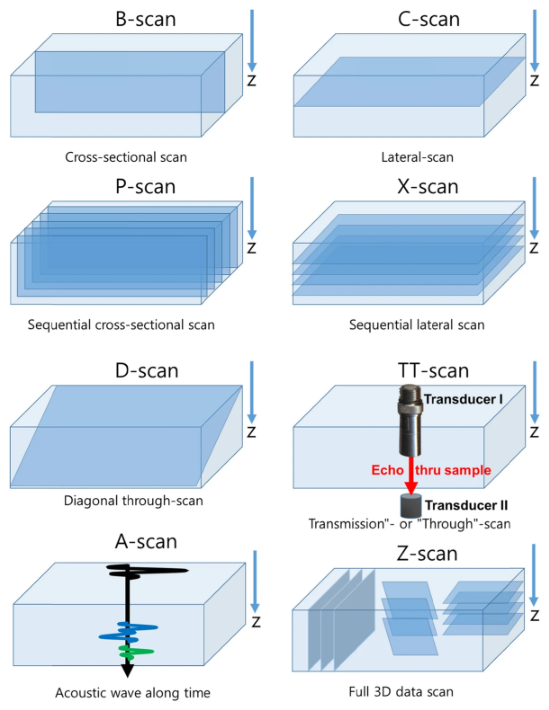
Figure 2.
Representative SAM B-scan acquired along a path crossing the three regions of the MICROSURF 334 reference plate with nominal values of , 25, and . The surface echo shows progressively greater vertical variation and irregularity as the nominal surface roughness increases.
Figure 2.
Representative SAM B-scan acquired along a path crossing the three regions of the MICROSURF 334 reference plate with nominal values of , 25, and . The surface echo shows progressively greater vertical variation and irregularity as the nominal surface roughness increases.

Figure 3.
Overview of the proposed pipeline for extracting and evaluating surface roughness from SAM B-scan images.
Figure 3.
Overview of the proposed pipeline for extracting and evaluating surface roughness from SAM B-scan images.

Figure 4.
Samples and measurement arrangements used for SAM image acquisition: (a) MICROSURF 334 reference plate; (b) SAM image acquisition from the standards specimen; and (c) SAM image acquisition from an additively manufactured cubic specimen.
Figure 4.
Samples and measurement arrangements used for SAM image acquisition: (a) MICROSURF 334 reference plate; (b) SAM image acquisition from the standards specimen; and (c) SAM image acquisition from an additively manufactured cubic specimen.
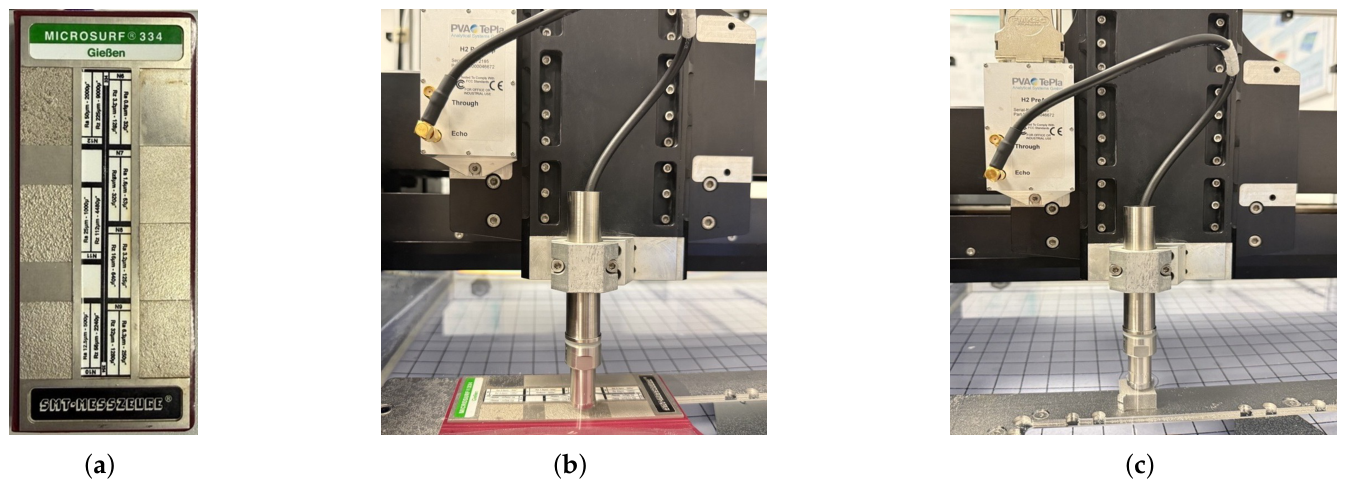
Figure 5.
Influence of the transducer position on acoustic focusing and the reflected signal: (a) under-focused, focused, and over-focused positions of the specimen surface relative to the focal plane; and (b) variation in the reflected signal intensity with the axial (z) transducer distanse to sample, where the maximum intensity is obtained at the focal position (2).
Figure 5.
Influence of the transducer position on acoustic focusing and the reflected signal: (a) under-focused, focused, and over-focused positions of the specimen surface relative to the focal plane; and (b) variation in the reflected signal intensity with the axial (z) transducer distanse to sample, where the maximum intensity is obtained at the focal position (2).
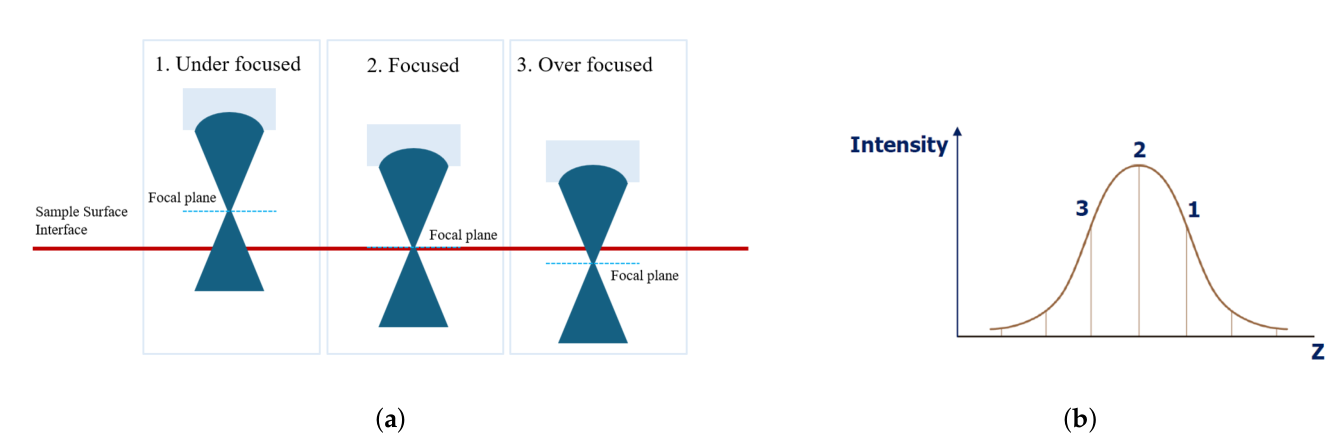
Figure 6.
WinSAM 8 interface showing the main acquisition settings and the percentage scale used to monitor the gated surface-echo amplitude during adjustment of the transducer focus and receiver gain.
Figure 6.
WinSAM 8 interface showing the main acquisition settings and the percentage scale used to monitor the gated surface-echo amplitude during adjustment of the transducer focus and receiver gain.
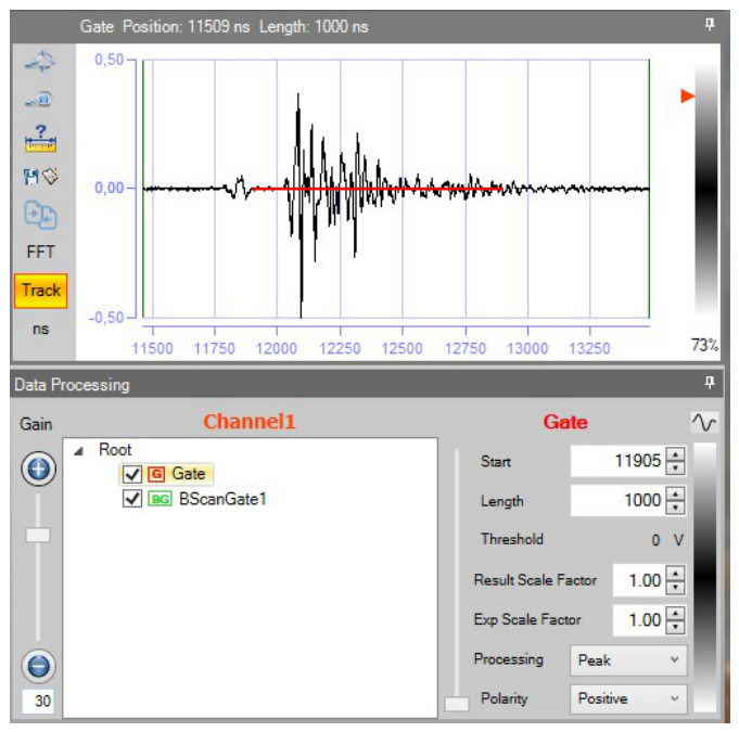
Figure 7.
Surface-profile extraction from a representative SAM B-scan: (a) original B-scan image; (b) detected water–specimen interface overlaid on the original B-scan; and (c) extracted surface profile in pixel coordinates.
Figure 7.
Surface-profile extraction from a representative SAM B-scan: (a) original B-scan image; (b) detected water–specimen interface overlaid on the original B-scan; and (c) extracted surface profile in pixel coordinates.
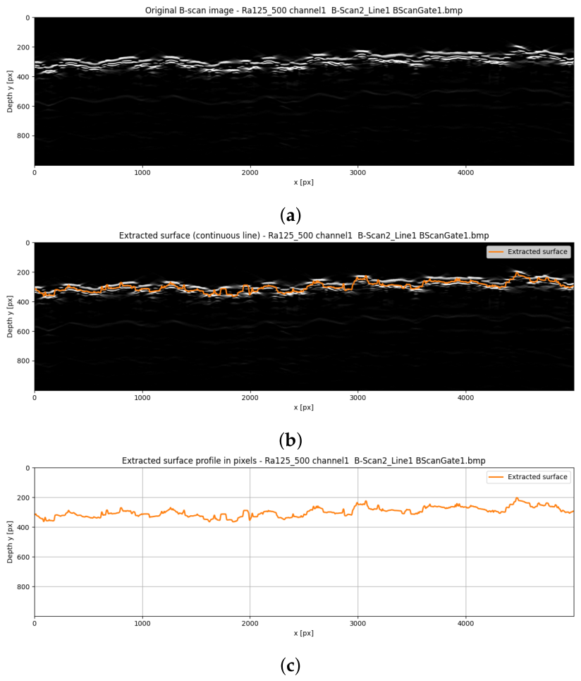
Figure 8.
Example of the filtering and form-removal procedure: (a) initial surface profile (blue), S-filtered profile (orange), and large-scale waviness profile obtained using the L-filter (green); (b) roughness-band profile after S- and L-filtering (blue) and fitted linear form used in the F-operation (orange); and (c) final roughness profile after removal of the fitted linear form.
Figure 8.
Example of the filtering and form-removal procedure: (a) initial surface profile (blue), S-filtered profile (orange), and large-scale waviness profile obtained using the L-filter (green); (b) roughness-band profile after S- and L-filtering (blue) and fitted linear form used in the F-operation (orange); and (c) final roughness profile after removal of the fitted linear form.
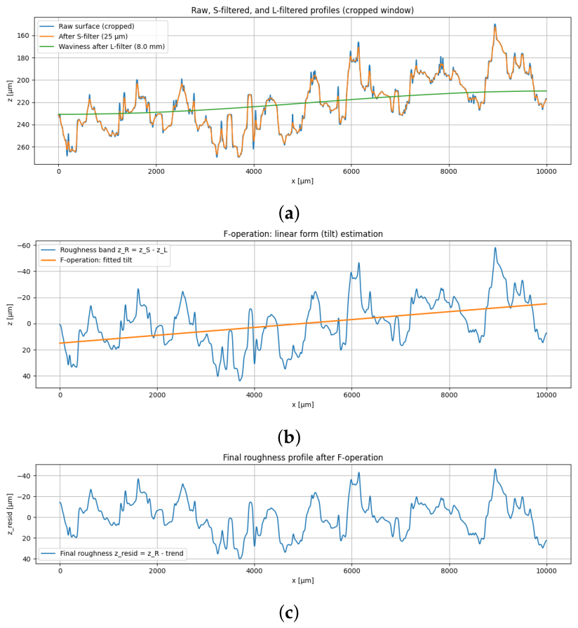
Figure 9.
Schematic representation of the profile roughness parameters , , , , and .
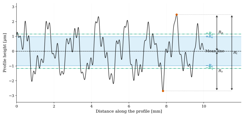
Figure 10.
Spatial sampling strategy used for the area-based surface roughness evaluation: (a) SAM C-scan of the complete measurement area; (b) location of one selected B-scan measurement line; and (c) positions of the 500 parallel B-scans acquired at a spatial offset of .
Figure 10.
Spatial sampling strategy used for the area-based surface roughness evaluation: (a) SAM C-scan of the complete measurement area; (b) location of one selected B-scan measurement line; and (c) positions of the 500 parallel B-scans acquired at a spatial offset of .
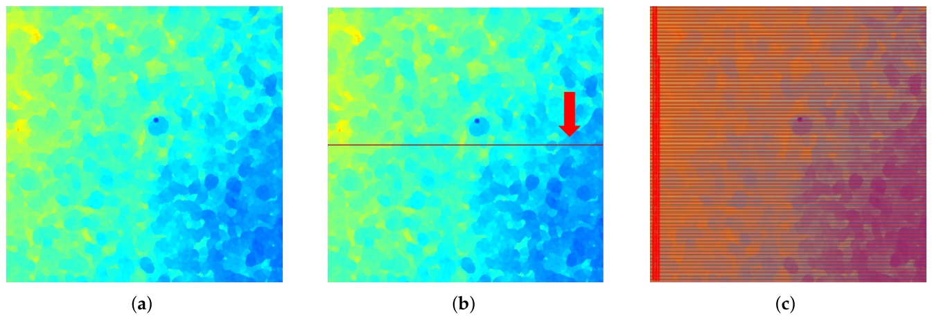
Figure 11.
Repeatability of the SAM-based measurements for the reference specimens with nominal values of (a) , (b) , and (c) .
Figure 11.
Repeatability of the SAM-based measurements for the reference specimens with nominal values of (a) , (b) , and (c) .
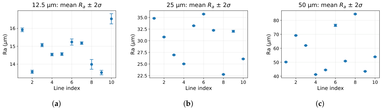

Table 1.
Comparison of the values obtained using the three measurement methods with the nominal values of the reference specimens.
Table 1.
Comparison of the values obtained using the three measurement methods with the nominal values of the reference specimens.
| Nominal | Method | Measured | Absolute deviation | Relative deviation |
|---|---|---|---|---|
| () | () | () | (%) | |
| SAM | ||||
| VHX-7000 | ||||
| VK-X3050 | ||||
| 25 | SAM | |||
| 25 | VHX-7000 | |||
| 25 | VK-X3050 | |||
| 50 | SAM | |||
| 50 | VHX-7000 | |||
| 50 | VK-X3050 |
Table 2.
Summary of the SAM repeatability results obtained from the fixed measurement lines.
| Nominal | Lines | Repeats per line | Mean of line means | Mean standard deviation | Mean |
|---|---|---|---|---|---|
| () | () | () | (%) | ||
| 10 | 21 | ||||
| 25 | 10 | 26 | |||
| 50 | 10 | 21 |
Table 3.
Comparison of the values measured on the additively manufactured cubic specimens.
| Specimen | SAM | VHX-7000 | VK-X3050 |
|---|---|---|---|
| () | () | () | |
| Cube 1 | |||
| Cube 2 | |||
| Cube 3 |
Disclaimer/Publisher’s Note: The statements, opinions and data contained in all publications are solely those of the individual author(s) and contributor(s) and not of MDPI and/or the editor(s). MDPI and/or the editor(s) disclaim responsibility for any injury to people or property resulting from any ideas, methods, instructions or products referred to in the content. |
© 2026 by the authors. Licensee MDPI, Basel, Switzerland. This article is an open access article distributed under the terms and conditions of the Creative Commons Attribution (CC BY) license.
Copyright: This open access article is published under a Creative Commons CC BY 4.0 license, which permit the free download, distribution, and reuse, provided that the author and preprint are cited in any reuse.