

Submitted:
08 October 2026
Posted:
10 October 2026
You are already at the latest version
Abstract
Foundation models and AI agents are increasingly used to read operational requests, estimate uncertain quantities, and draft plans. In supply chains, these outputs feed decisions that must respect costs, stock and capacity limits, and business rules, and whose effects become visible only after delayed and often partial execution. This perspective, ScoAI = SC + OR + AI, argues that learned components should be designed around the decision they support. Supply-chain context defines the problem, operations research supplies objectives, constraints, and coordination, and AI supplies estimates and judgments that can be reused across tasks. We call a model or agent OR-native when these elements are explicit in its interface, and we refer to the coupling of learned components with executable operational relations as data--mechanism fusion. The coupling can fail in three places: when a judgment is turned into an action, when a locally good choice changes the cost of later stages, and when the executed action differs from the approved one. For each, we give a short analysis. Cost-sensitive thresholds and a decomposition of decision loss address the first; completion values and resource prices address the second; and a censoring argument shows how executed actions limit what operational logs can teach. Systems developed at JD.com illustrate these interfaces, and small constructed examples make every calculation reproducible. We close with decision records, an agent architecture, and evaluation protocols that compare reusable components with specialist workflows on decision quality, validity, coverage, and total cost.
Keywords:
ScoAI
; OR-native models
; decision intelligence
; data-mechanism fusion
; supply chains
1. Introduction
Consider a supplier message warning that an inbound shipment for a promoted item may arrive late. The planner can expedite the shipment, move stock from another warehouse, or wait. Choosing well requires an estimate of the delay risk, the cost of each response, the stock and transport capacity that each response consumes, and the rules that apply to this supplier and promotion. After the choice is made, the shipment may still arrive partly or late, and sales during a stockout reveal only that demand exceeded the available stock. A good forecast is one input to this decision, but it does not settle it.
Foundation models and agents can now help with several of these steps. They can read the message, retrieve the relevant rules, write or adapt an optimization model, estimate responses, and call tools [1,2]. Some recent models return typed outputs instead of prose: a choice among supplied options, a rating on a declared rubric, or a probability for a stated proposition [3,4]. Such outputs are easy for software to consume. They do not, by themselves, say what a score means in cost terms, which constraints the resulting action must satisfy, or how its effect will be checked once it is carried out.
Operations research has long addressed part of this problem. Predictive-to-prescriptive analytics and decision-focused learning tie the estimation target to the optimization model that uses the estimate [5,6,7]. In these settings, an analyst fixes the prediction target and the optimization model in advance. A reusable model or an agent instead decides, task by task, what to estimate, which formulation to build, and when to act. The decision structure therefore has to travel with the model: it must be visible in the interface between learned components and the computations that consume them, rather than being supplied separately by the analyst for each application.
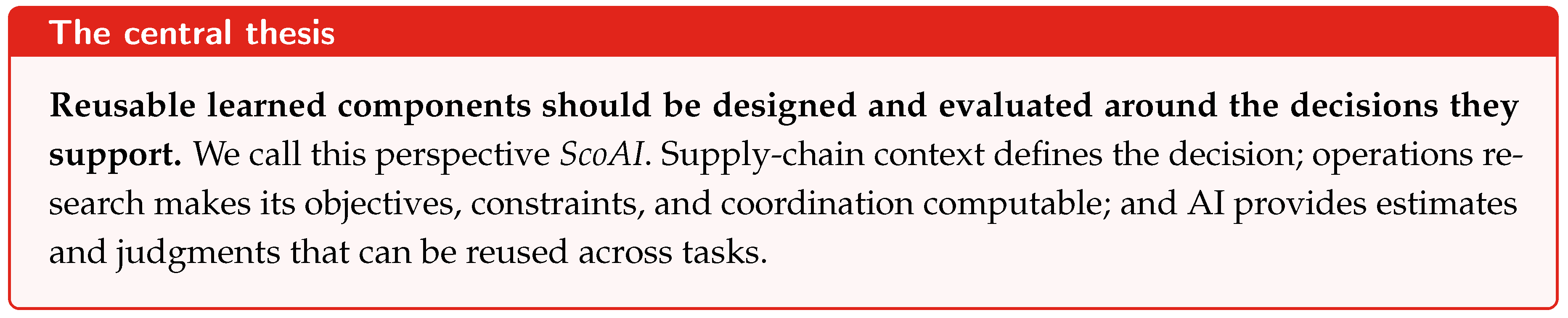
We call a model or agent OR-native when objectives, admissible actions, uncertainty, information, and feedback are explicit parts of its interface. The term refers to this interface requirement, not to a particular neural architecture or to the mere ability to call a solver. We refer to the coupling between learned components and executable operational relations as data–mechanism fusion. In inventory, for example, material balance can be applied exactly, demand response must be estimated, and the solver allocates stock among competing uses. Fusion lets each part do what it does reliably and lets information flow between them: decision costs can guide estimation, conservation relations can structure learned dynamics, solver feedback can improve formulations, and executed outcomes can update the uncertain components. The name ScoAI also suggests score; we use it as a reminder that a score is an input to a decision rather than the decision itself.
1.1. Three Gaps Between a Judgment and Its Execution
The delay example shows three places where a learned output and an operational decision can come apart.
The first lies between a judgment and an action. A delay probability of 10% makes “no delay” the most likely outcome, yet expediting can still be the cheaper response when a stockout is costly; Section 3.1 works through such a case. Likewise, the plan rated highest by a model may exceed the stock or capacity available. Probabilities, rubric scores, confidence values, and expected costs are different quantities, and each needs its own interpretation and test before it can drive an action.
The second lies between local and system-level value. Expediting into one warehouse uses transport and receiving capacity that other replenishment decisions rely on, and an assortment choice changes the replenishment and routing problems that follow it. A stage that minimizes its own cost can raise the cost of the complete plan.
The third lies between the approved plan and what is executed. Partial dispatch, late receipts, and human overrides determine the state that is actually reached. The data that follow also depend on execution: when stock runs out, recorded sales understate demand. A learning system that treats its recommendations as executed, or its sales as demand, will evaluate and train itself on the wrong quantities.
Existing work addresses parts of these gaps. ORLM, OptMATH, and OptiRepair connect language, formulations, and solver feedback [8,9,10,11]. Learned search and multi-task optimization reuse computational structure across instances [12,13,14]. Planning agents and OR-guided inventory learning connect such components to operating systems [15,16,17,18,19]. These studies usually examine one interface at a time. Less is known about how to combine them so that objectives, feasibility, information, and feedback remain consistent from the learned output through to the executed action.
1.2. Contributions and Organization
This perspective makes four contributions.
- 1.
- It defines ScoAI, the OR-native requirement, and data–mechanism fusion, and lists the interfaces through which learned and mechanistic components exchange information (Section 2).
- 2.
- It analyzes each gap in turn (Section 3, with proofs in Appendix A). For the first, it links score semantics to consequence costs and splits decision loss into three parts: candidates that were never considered, errors in comparing candidates, and incomplete search. For the second, it uses completion values and resource prices to carry downstream consequences back to earlier stages. For the third, it shows how executed actions and censored observations limit what logs can identify.
- 3.
- It specifies decision records that link the decision specification, scores, proposed, approved, and executed actions, and outcomes, together with an agent architecture in which judgment, computation, commitment, and learning can be tested separately (Sections 4–6).
- 4.
- It maps systems developed at JD.com and a constructed inventory system onto these interfaces, and derives evaluation protocols and research priorities from the same analysis (Sections 7–9).
The evidence is of three kinds, and we keep them separate. The JD.com systems are reported with their original study designs and metrics; several authors of this perspective contributed to them, and their results are cited rather than replicated. The constructed disruption and inventory examples are small enough to verify by hand. Product documentation of structured judgment models motivates a proposed integration and test protocol; we report no experiment with, or supply-chain deployment of, such a model. Proof assumptions and reporting boundaries are collected in Appendices Appendix A and Appendix B, and Figure 1 summarizes the decision loop that the paper follows.
2. Decision Interfaces and Operational Mechanisms
2.1. ScoAI and the OR-Native Design Requirement
ScoAI = SC + OR + AI names the three sources of a decision system introduced in Section 1. The supply chain contributes resources, actors, information, and the consequences of actions. Operations research contributes objectives, uncertainty models, constraints, and coordinated computation. AI contributes estimates, interpretations of context, and statistical and computational knowledge that transfer across tasks. The three interact: a demand estimate is only as useful as the cost model that weighs its errors, and a cost model is only as useful as the estimates fed into it.

Supply chains anchor the discussion, but the same interface principles carry over to other domains in which decisions compete for limited resources. The perspective concerns system design rather than a particular checkpoint, solver, or product. The rest of this section distinguishes three kinds of mechanism, states a common mathematical form, and then gives a precise definition of data–mechanism fusion.
2.2. Three Kinds of Mechanism
In this perspective, a mechanism is an explicit relation used to describe or control a decision system. Three kinds require different treatment.
- Physical and accounting relations.
Material balance, inventory transitions, travel-time accumulation, and resource consumption define how states and actions fit together. Under the specified system boundary, these relations can be implemented directly. For example, selling one unit reduces on-hand stock by one unit; this coefficient need not be estimated from transaction logs.
- Decision and institutional structure.
Capacity, compatibility, integrality, precedence, service definitions, and cost functions specify the admissible choices and their evaluation. Some are stable; others change with contracts or operating policies. They belong in a versioned decision specification that can be supplied to a model and executed by tools.
- Empirical response relations.
Demand response, lead-time distributions, substitution, and supplier behavior link actions and context to uncertain outcomes. Their form may reflect domain knowledge, while their parameters or residual variation are learned from data. They require estimation and revision as operating conditions change.
Each kind calls for a different computational treatment: accounting relations are enforced, current decision rules are applied, and empirical responses are estimated and revised. Theory-guided and scientific machine learning provide related ways to combine structural knowledge with estimation [20,21,22]. OR adds explicit objectives, feasible sets, information constraints, and optimization feedback.
2.3. A Common Mathematical Interface
Let be the information available at decision time t, the active mechanism version, and the operational state, including outstanding commitments. A fused sequential computation takes the form
Here supplies uncertain inputs and may include a belief over unobserved state; applies the structural transition; gives the current admissible action set; and contains policies respecting the available information and specified constraints under the version sequence . The expectation includes the observation process and subsequent policy responses. For partially observed hard restrictions, admissibility is defined over the specified state support. Static optimization is the single-decision case, with no transition model required. These equations idealize faithful execution; when dispatch differs from the approved plan, the transition uses the recorded executed action (Sections 3.7 and 7.6).
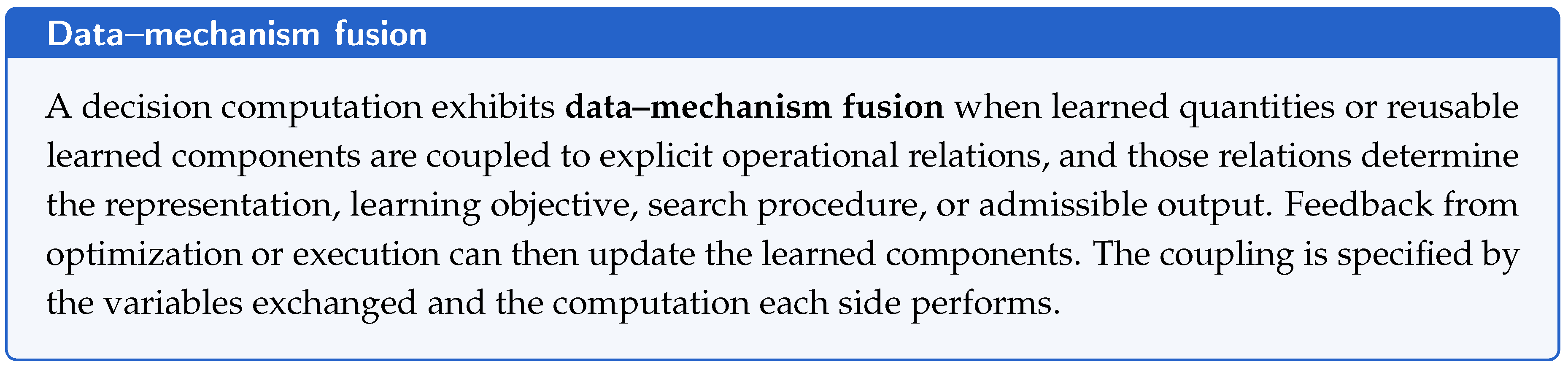
The learned object can be a conditional distribution, a decision score, a value function, a formulation, a candidate generator, or a search policy. A foundation model reuses such objects across a task family [1,2]; an agent combines them with current data, solvers, simulators, and information requests. Structured output alone does not establish an OR-native interface: the outputs must connect to an objective, admissibility conditions, and independent assessment. A foundation-model claim additionally requires evidence of reuse across a stated task family.
2.4. Where the Coupling Enters
The interfaces below specify what a learned component exchanges with an operational model and how that information enters the computation.

Table 1.
Interfaces between learning and operational mechanisms. These interfaces can coexist; none alone establishes end-to-end decision quality.
Table 1.
Interfaces between learning and operational mechanisms. These interfaces can coexist; none alone establishes end-to-end decision quality.
| Interface | Learned contribution | Mechanistic contribution and feedback |
|---|---|---|
| Representation | Context, demand beliefs, graph embeddings | Typed entities, flow structure, domains, and shared resource identities |
| Training | Predictors, policies, and formulation models | Decision losses, OR-generated labels, feasibility witnesses, and solver feedback |
| Inference | Probabilities, scores, candidates, and search guidance | Constrained optimization, exact state updates, bounds, and scenario accounting |
| Operational update | Response and policy adaptation | Executed-action records, observation models, revised rules, and reconciliation |
In a one-way pipeline, a predictor is trained for statistical fit and its output is passed to an optimizer. In decision-focused fusion, the optimizer’s loss also shapes the predictor. In structured dynamics, a learned distribution supplies shocks to an exact transition. In solver-in-the-loop learning, optimization outputs supervise subsequent proposals. These choices address different sources of error and can be compared separately.
For a static task, the local interface can be recorded as
where gives entities and units, specifies uncertainty and risk treatment, and records acceptance requirements, deadlines, and fallback conditions. The admissible set is the one in ; it may also depend on , for example through robust or chance constraints. A rule change then updates only the relevant part of , while reusable learned parameters stay fixed, so the effect of the change can be tested in isolation.
2.5. Precision Follows the Operational Relation
Fusion places different precision requirements at different interfaces. Accounting identities and discrete domains are implemented directly. Continuous inequalities are checked in physical units. Service probabilities and fill rates are evaluated under their specified distributions and horizons. Execution is reconciled against the approved action and current resource availability.
For a continuous inequality, let be a planned guard margin, a numerical residual allowance, a bound on constraint-model discrepancy, and a bound on the effect of execution perturbation. The sufficient condition
preserves that inequality under the assumptions proved in Appendix A.4. All terms have the same residual units. Integer case packs require a domain check, and exact flow equalities require a consistent update; neither is replaced by a larger continuous margin.
3. From Scores to Decisions: Value, Feasibility, and Coordination
An operational decision combines an estimate, a consequence model, and a feasible computation. This section follows the three gaps of Section 1. For the gap between judgment and action, we connect scores to actions (Section 3.1) and then distinguish three sources of improvement: better estimation (Section 3.2), better value comparisons (Section 3.3), and admissible search (Section 3.4 and Section 3.5). For the gap between local quality and system value, completion values and resource prices coordinate stages (Section 3.6). For the gap between a plan and its execution, executed actions and their observation mechanism determine the next state and the next data (Section 3.7). The economics of reuse closes the section (Section 3.8).
3.1. A Score Needs a Decision Interpretation
A probability, a rubric rating, and an expected operational cost are different objects (Table 2). A distribution over candidate answers expresses a model’s judgment within the supplied choice set and rubric. It is not automatically a probability of physical success, a cardinal utility, or an optimality certificate. Numeric output removes a parsing problem; its decision meaning still has to be specified.
For a static decision with total consequence cost , a typical conversion is
Here is the retained candidate set and the independently specified admissible set. If their intersection is empty, the system must generate new candidates or use an authorized fallback. Risk-sensitive objectives and service constraints require their own declared semantics; sequential decisions additionally value nonanticipative continuations. Neither candidate probabilities nor rubric scores can be substituted for without validating that interpretation.
Consider a constructed binary disruption decision. A disruption has probability p, incurs loss 100 if no action is taken, and is fully prevented by an expedite action costing 6. Expediting is optimal when
At , “no disruption” is the most likely outcome, yet expediting costs 6 rather than an expected 10. A 0.5 classification threshold would give the wrong action. This example isolates the role of consequences; it does not assume that expediting always prevents disruption in an actual supply chain. Appendix A.1 gives a regret calculation and a separate example of equal rubric averages with unequal consequence costs.
Probabilistic calibration and proper scoring rules assess a specified predictive target [23,24]. They do not supply its costs or constraints, and the cost-minimizing action need not be the one the model is most confident about. A structured judgment model (Section 4.5) can therefore supply a calibrated input to Equation 6, but the action is chosen by Equation (7).
3.2. Correct Structure Reduces the Learning Problem
Suppose the state update has a known accounting component and an unknown response component. Instead of estimating an unrestricted transition, construct
For inventory, can generate nonnegative demand and positive integer lead times, while updates sales, on-hand stock, and pipeline inventory. Conservation then holds for every admissible generated input, including combinations absent from the training set. Statistical effort is concentrated on demand and delay rather than spent reconstructing bookkeeping.
A finite-class argument makes the estimation benefit explicit. Let be a finite predictor class and a class fixed by a supplied mechanism before observing the training sample. In the inventory case, contains unrestricted transition predictors and contains only those of the form Equation (9). For independent identically distributed samples and , loss in , population risk R, and empirical risk minimizer , with probability at least ,
Here is the best risk in the reference class. The proof in Appendix A.2 uses uniform concentration. The right-hand side is a guarantee, not the realized error. If the restriction is correct, in the sense that contains a best predictor in , the approximation bias is zero and the smaller reduces the sample size needed for a given guarantee. If it is wrong, the bias is positive and does not shrink with more data. Known conservation relations should therefore be encoded firmly, and assumptions about empirical response kept open to revision. For neural classes, the relevant complexity measure changes; the same bias–estimation tradeoff remains the design question.
3.3. Decision Costs Determine Which Predictions Are Useful
Statistical accuracy and decision quality weight errors differently. For stock , nonnegative demand D of finite mean, and costs , the one-period inventory problem is
where is the distribution function of D. The optimum is therefore a demand quantile, and the cost ratio selects which one. For , constant demand of one gives . Demand equal to five with probability and zero otherwise has the same mean, but gives . Choosing its mean costs , compared with cost 4 at . A mean predictor can be statistically correct while omitting the information needed by the decision.
Decision-focused training addresses this mismatch by composing prediction and optimization [6,7,25]:
The realized decision loss sends information about capacity, costs, and tradeoffs back to the statistical model. A prediction-only loss omits this feedback even when an optimizer is used after training.
For a concrete differentiable interface, consider subject to , where , A has full row rank, are fixed, and is differentiable. With optimal solution and equality multiplier , differentiating the optimality conditions gives
The constraint matrix A appears in the system, so the gradient passed back to moves the decision only in directions that keep . Differentiable optimization layers implement such couplings [26,27]. With inequalities the same local calculation requires a stable active set and regularity; discrete problems instead motivate surrogates, perturbations, or solver-based training signals.
3.4. Mechanisms Should Enter the Feasible Computation
Better estimates and decision-aware training improve value comparisons; they do not by themselves make the selected action admissible.
For a proposal and a nonempty closed feasible set , an exact projection satisfies
Constrained decoding, optimization layers, and feasible incumbents offer related ways to implement the same division of labor: learning proposes or ranks, while the constrained computation produces an admissible action. Projection can change decision value, so the resulting action is evaluated after projection.
A quadratic violation penalty need not enforce the same feasible set. The problem , for any finite , has minimizer , although the desired hard constraint is . Penalizing violations can guide learning without implementing the feasible set. The choice between a hard interface and a soft loss therefore follows the meaning of the relation being encoded.
3.5. Separate Representation, Valuation, and Search
Fix an objective, horizon, information structure, and feasible policy class . A learned representation or candidate generator retains a nonempty class . Define
The first term is the value lost by restricting choices; the second is the largest distortion of a pairwise cost comparison.
Proposition 1
(Decision loss of restricted planning). Assume that J and are real-valued on , that , and that . If is within of the minimum learned cost over , then
Uniform value error at most ε implies .
Appendix A.5 proves the result. Mechanism-aware representations can retain useful choices and reduce ; decision-focused learning can reduce ; and better optimization can reduce . Improving one term does not reduce the others: exact search over a poor candidate class leaves and unchanged. The feasibility premise is supplied by the decision interface, not by the value-error bound. For a scoring model, the corresponding tests are candidate coverage, value ranking, and action selection. Evaluating them separately identifies whether better generation, estimation, or computation is the useful next intervention.
3.6. Cross-Stage Value Is the Object to Coordinate
For task context z and coupled decisions , define the completion value of a partial plan by
with value when no feasible completion exists. Because an infimum over a product of choices can be taken one stage at a time, on feasible plans and , where ranges over choices with a feasible continuation. When these infima are attained, choosing and then each yields a plan of cost . A stage that minimizes only its own cost drops the downstream term of this recursion.
This formulation is for a deterministic decision pipeline; under uncertainty, the remaining choices are nonanticipative policies and the objective is their conditional expected cost. An assortment decision is then valued through the replenishment, fulfillment, and routing choices it enables. For example, an upstream option with local cost 1 and best downstream cost 8 is worse than an option with costs 3 and 1. Local optimization selects total cost 9; completion-value optimization selects total cost 4.
Resource prices provide a second coordination interface. Consider the coupled problem
with optimal value . Assume convex and , and a Lagrangian saddle point with , as holds under a Slater condition. Then a plan is optimal exactly when it minimizes the local terms at the common prices, satisfies the coupling constraint, and satisfies complementary slackness. Local minimization alone is not sufficient: when local minimizers are not unique, as in linear programs, some of them can violate the coupling constraint. The prices also bound the value of capacity,
so is a subgradient of the convex function , and where is differentiable. Thus a shared capacity has a marginal value that can enter local training targets or policy inputs. Integer decisions can retain a duality gap; the same prices then supply bounds and coordination signals, while the final plan still comes from the coupled feasible problem. Multi-echelon inventory theory and information-sharing research provide the operational background for these interfaces [28,29,30].
3.7. Executed Actions Determine the Next State and the Next Data
The preceding results value an action as if it were carried out as chosen. In operation, an approved action passes through reservations, partial dispatch, and human overrides before it becomes the executed action . With an execution channel and observation model ,
Two consequences follow. First, the cost of a planning policy is its expected cost through : when execution deviates systematically, the realized policy differs from the evaluated one, and the transition must use the recorded rather than the plan. Second, executed actions determine what can be learned. With demand and available stock , sales equal , so availability censors demand. If historical availability never exceeds three, constant demands of three and five generate identical logs; for any stocking rule based on those logs, Proposition A2 shows that the larger of the two expected regrets under absolute-deviation cost is at least one. No estimator can remove this ambiguity; only an action that raises availability, or a record of unmet demand, can. The decision records of Section 5 and the commitment interface of Section 6 are designed around these two facts.
3.8. Reuse Changes the Economics of the Computation
For N uses of a learned component, express its fixed development cost , recurring computation and integration costs, and operational loss in common units:
Validity and useful coverage are reported alongside this cost. If denotes the event that an output is accepted and that it violates a hard obligation, require
These dimensions define the supported-decision frontier in Figure 1. Compare a reusable workflow with a dedicated workflow built for one task family, with fixed costs and and expected recurring costs per use , the latter being the expectation in Equation (22) for each workflow. At equal expected operational loss, validity, and coverage, the reusable workflow has lower average cost exactly when
When the reusable component is shared across several task families, is the share allocated to the family under study. Mechanism reuse can reduce specification and checking effort as well as search time. Local adaptation and exception handling contribute to the same comparison. This makes structural transfer and total decision cost the economic tests of a foundation-model strategy. Cheap scoring is beneficial when it reduces this end-to-end cost at comparable quality and coverage; a lower model-call cost alone does not establish the benefit. The literature reviewed next supplies reusable components for each of these computational roles.
4. Research Landscape: Reusable Models, Judgments, and Computation
The literature can be organized by the object learned, the mechanism supplied, and the feedback exchanged between them. This view connects learned optimization [31,32], decision-focused learning [7], and LLM-based formulation, algorithm design, and validation [33]. Each strand implements a different interface in Table 1. Organizing the work by its computational role clarifies what can be reused and what still needs task-specific specification.
4.1. Classical Decision Models Supply the Computational Structure
Stochastic programming specifies scenarios and nonanticipativity; robust optimization specifies uncertainty sets and protection requirements; dynamic programming specifies value recursion; and model predictive control repeatedly solves a finite-horizon problem using updated state information [34,35,36,37]. These structures determine how learned forecasts, values, or transitions enter a decision. Approximate dynamic programming also makes the tradeoff between value approximation and computation explicit [38].
Supply-chain theory adds the structure of multi-echelon control, coordination, and information propagation [28,29,30,39,40]. Foundation-model reuse operates on top of these decision relations: it can estimate uncertain inputs, amortize expensive computations, and adapt recurring formulations to new contexts.
4.2. Formulation Models Couple Language to Executable Mechanisms
NL4Opt makes the extraction of optimization structure an explicit benchmark [41]. OptiMUS connects language-based modeling to mixed-integer linear programming, and ORLM trains models for customizable automated formulation [8,42]. OptMATH uses bidirectional synthesis and filtering to produce paired problem descriptions and mathematical models; autoformulation with search explores candidate formulations and removes symbolic redundancies [9,43]. In this interface, the mechanism is both the learning target and the executable object used to assess proposals.
OptiMind uses class-specific error analysis in training-data cleaning and inference [44]. OptiRepair combines solver diagnosis with inventory rationality checks [10]. These approaches send mathematical and domain feedback back into formulation. OptiGuide places an existing optimization model behind a natural-language what-if interface [15], allowing business context to select a structured computation.
The assessment target matters. Executability checks program behavior; feasibility checks the modeled constraints; comparison to accepted requirements checks the formulation. Optimal-value agreement, used in ORLM evaluation and OptMATH filtering, is useful but does not distinguish every pair of feasible sets. For example, minimizing x over or gives the same optimum, while minimizing separates them. Objective perturbations and constraint witnesses therefore complement value-based feedback.
4.3. Learned Optimization Couples Proposals to Search Structure
Neural construction policies learn solution patterns, while learned branching policies guide a structured search [12,45,46,47]. A branching policy that changes only the search order can use a sound branch-and-bound procedure to retain exactness. The learned contribution is computational efficiency under the instance distribution and algorithm class being studied [48].
MVMoE combines a shared routing representation with constraint-specific masks, training on six variants and evaluating ten unseen combinations [13]. MILP-Evolve generates diverse MILP classes for pretraining and studies gap prediction, branching, and language–MILP alignment; its MIPLIB transfer experiments include task-specific fine-tuning [14]. These methods make constraint structure part of the representation and the transfer protocol.
Evolution of Heuristics, MCTS-AHD, and FunSearch use executable feedback to search for reusable programs [49,50,51]. The output of learning can thus be an algorithm that is reused across many decisions. Its evaluator and program skeleton supply mechanistic structure, while the generative model explores alternatives.
4.4. Decision-focused Learning Couples Estimation to Value
Predictive-to-prescriptive analytics uses covariates to construct decision models; decision-focused training accounts for the downstream cost of the predictions [5,6,7,25]. Differentiable optimization layers make this coupling computationally explicit, as in Equation (13) [26,27]. The key feedback is the effect of a prediction on the chosen action, not its error considered in isolation.
Mechanisms can also contain quantities to be inferred. Inverse optimization learns decision-model elements from observed choices. Ren et al., for example, learn signal-dependent feasible regions using specified conic primitives and known linear objectives [52]. This provides a structured hypothesis class for learning constraints. Its interpretation depends on the assumptions connecting observed actions to the underlying objective and feasible set.
4.5. Structured Judgment Models: Explicit Choices and Scores
A structured judgment model answers a bounded question about supplied state with a typed output and a distribution, rather than with prose. Its outputs are meant to be consumed by software: a selection among supplied options, a rating against declared rubric levels, or a probability for a stated proposition. Reading context thus produces a number with a declared meaning rather than free text. Such a model can assess an exception, compare stated options, or supply a learned input to a policy, while numerical and optimization tools handle arithmetic, feasibility, and the final choice.
TypeSafe’s Jev is a documented instance, described by its developer as a System One model. Its primitives are Choice, a selection with a distribution over supplied options; Score, a rubric-based rating with a level distribution; and Noul, a yes/no probability judgment on a statement. The launch announcement describes Reinforcement Learning for Calibrated Decisions (RLCD) as its training approach [3]. Calibration concerns the probability of a specified answer or event, whereas decision-focused learning also incorporates consequences; calibration in a new operating population requires testing. The account here relies on the announcement and its accompanying first-party documentation, accessed on October 8, 2026.
The returned numbers have different definitions. With level probabilities , Score returns the mean level number; for Choice options, the documented confidence is a rescaled maximum probability:
Thus a binary Choice with probabilities has confidence 0.8, not 0.9. The statistic describes the returned distribution, not a guaranteed probability of correctness. Score uses a separate order-sensitive confidence statistic, and Noul returns a yes probability without a separate confidence field. These distinctions matter when composing scores, choosing thresholds, or auditing an automated action (Table 2).
The documentation for jev-1.13, last reviewed October 2, 2026, notes limitations in numerical precision, date comparisons, and option-order sensitivity, and cautions against reconstructing exact magnitudes from rubric expectations [3]. In a replenishment system, a judgment model may therefore interpret a supplier message, while code checks receipt dates and a solver enforces shared stock, case packs, and capacity. A plausible judgment does not authorize relaxing those constraints. The operational contribution of any such model depends on the connection from its outputs to costs and admissibility in Equations (6) and (7); Sections 6 and 8.2; propose an adapter and evaluation protocol for that connection. No hosted-model experiment or deployment result is claimed here.
4.6. World Models Couple Learned Response to Planning
Bounded judgments describe one interaction; sequential planning also requires reasoning about how actions change future states and observations. Decision Transformer and Trajectory Transformer learn from decision sequences, using different conditioning and planning procedures [53,54]. Surveys of decision foundation models describe broader pretraining and adaptation opportunities [2,55]. Offline policy learning connects these representations to questions of action support and the information contained in logged trajectories [56].
World Models, MuZero, and Dreamer learn internal response or value models for control [57,58,59]. Value-aware model learning targets the values queried by a planner, and value equivalence formalizes agreement relative to chosen policies and function classes [60,61]. These are direct antecedents of the decision-comparison term in Equation (17).
Richens et al. relate competence over specified composite goals to recoverable transition information in a finite, stationary, fully observed controlled Markov setting [62]. Vafa et al. probe learned structure through inductive bias [63], while pretraining scaling work studies how agent and world-model performance changes with resources [64]. For supply chains, the corresponding questions are which response information transfers, which structural relations remain explicit, and how much decision cost the representation saves. Reusing one training algorithm across tasks and transferring one pretrained checkpoint are distinct experimental protocols.
4.7. Structured Dynamics and Operational Observations Close the Loop
Theory-guided and geometric learning inject structure through hypothesis classes, representations, architectures, and losses [20,21,22]. Neurosymbolic world models and constrained reinforcement learning connect structured response models with policy learning [65,66,67]. PIGDreamer uses privileged training information in partially observed safe control [68]. The relevant interfaces distinguish per-action feasibility, expected-cost constraints, model mismatch, and information available only during training.
Digital twins synchronize models with operational systems and integrate data, simulation, and decision tools [69,70,71]. Simulation optimization provides an established way to search within such environments [72]. A reusable model can contribute response priors or computational policies while the local twin maintains system-specific state and mechanisms.
Inventory control connects these ideas to action-dependent observation. Nonparametric learning with censored demand accounts for the fact that stock limits what is observed [73,74]. Deep reinforcement learning has been studied across lost-sales, dual-sourcing, and multi-echelon problems [75]. In Zara’s allocation system, observed size-dependent display behavior changes how inventory translates into sales and therefore changes the optimization model [76]. These examples illustrate why the observation and response mechanisms belong in the learning problem.
4.8. Three Feedback Loops
The preceding methods use three distinct feedback loops (Figure 2). A formulation loop compiles, solves, diagnoses, and revises a model. An algorithm-design loop evaluates and improves a reusable heuristic. An operational loop executes a decision and incorporates the resulting events into the next decision. The first two can be nested inside the third. Their feedback has different meanings: solver feasibility, benchmark performance, and observed operational response. Keeping these targets separate also prevents a successful solver call from being mistaken for evidence of operational gain.
Planning agents orchestrate these interfaces [16]. OR-guided pretraining, solver-verified formulation selection, and coupled supply-chain policies place feedback at different points in the computation [17,77,78]. The JD.com portfolio in Section 7 examines these choices within one operational domain.
4.9. What the Different Forms of Evidence Establish
Table 3 compares the interfaces and evidence in representative work. Product documentation establishes an available interface; benchmarks test a computation; operational studies assess its use in a particular system. Each supports a different claim.
Table 3.
Representative learning–decision interfaces. Jev denotes documented functionality; other rows summarize studies.
Table 3.
Representative learning–decision interfaces. Jev denotes documented functionality; other rows summarize studies.
| Case | Interface used | Consequence for fusion |
|---|---|---|
| Structured judgment (Jev) [3] | Typed questions return choices, ratings, and distributions | Structured judgment still needs an explicit objective and admissibility checks |
| OptiGuide [15] | Business questions translated into queries around an existing fulfillment MIP | Query semantics select the optimization computation |
| OptiRepair [10] | Solver diagnosis and inventory rationality checks guide model repair | Different checks provide different training signals |
| MVMoE [13] | Shared routing attributes with feasibility masks | Learned transfer and explicit admissibility can be composed |
| FunSearch [51] | Generated scoring programs inside an executable algorithm skeleton | Search feedback produces a reusable algorithm |
| Zara [76] | Size-dependent display behavior embedded in an inventory-allocation MIP | An empirical response mechanism changes allocation value |
| UPS ORION [79] | Route optimization integrated with daily driver workflows | The useful decision includes execution timing and practices |
OptiGuide’s Azure fulfillment example makes the language–mechanism interface concrete: a request for earlier delivery must identify the reference date before code generation can answer the intended question. The report describes production integration with planners retaining business context and override capability ([15], Secs. 5–6).
OptiRepair supplies a within-system comparison of feedback signals. On its 284-problem held-out synthetic test set, GPT-5.2 achieves 53.5% feasibility recovery and 42.2% rational recovery; the trained Qwen3-8B pipeline reaches 81.7% rational recovery [10]. These figures concern the study’s specified repair protocol and inventory checks, including cost consistency and order smoothing. They support separating feasibility from operational validation and evaluating specialized training, not a general ranking of model families.
Zara supplies the corresponding mechanism lesson from allocation practice. When a major size is unavailable, an article can be removed from display, coupling sales across sizes. The model embeds this observed behavior through a sales approximation and a MIP. Its pilot used matched articles and a difference-in-differences analysis, with ten articles providing sufficient post-switch data [76]. Here empirical observation supplies the response structure that optimization uses.
The transferable object differs across these systems: a formulation pattern, a constraint-aware representation, a program, or an empirical response model. Training records must preserve the specification and feedback that give each object its meaning. This is the data-design problem developed next.
5. Learning from Mechanisms, Scores, and Decision Records
The interfaces in Section 4 require aligned evidence. A score needs a declared target; a formulation needs an accepted specification; an outcome needs the action and information that generated it. Training data should link these objects rather than store descriptions, scores, and outcomes as unrelated examples.
5.1. Represent the Same Decision Across Views
Natural language expresses intent and exceptions; algebra specifies variables and constraints; graphs expose network coupling; event records encode timing; and solver traces describe computation. Fusion requires these views to refer to the same entities, quantities, and rules. A model can then condition on mechanism structure, rather than infer each task solely from surface wording [26,27,32].
Consider a store dispatch cap changing from four units to two. The change updates an algebraic bound, a graph attribute, an action mask, and the simulator’s admissible inputs. It also changes which cached decisions remain feasible. Figure 3 shows these dependencies for the worked allocation in Section 7.6. The old feasible decision is invalidated, while the old lower bound survives because the objective is unchanged and the feasible set shrinks. Thus explicit structure supports selective reuse as well as correction.
Figure 3.
A cap edit in the constructed future-epoch allocation. Stocks and demand stay fixed; unit lost-sales and holding costs remain 10 and 1, with zero shipping and warehouse holding costs. Tightening store 2’s cap replaces by and leaves two warehouse units unused. Under the unchanged objective, feasible-set inclusion preserves the old lower bound of zero while the old decision becomes inadmissible. Algebra, graph, action mask, and simulator use the same updated cap. The old plan’s score cannot override the new admissibility condition.
Figure 3.
A cap edit in the constructed future-epoch allocation. Stocks and demand stay fixed; unit lost-sales and holding costs remain 10 and 1, with zero shipping and warehouse holding costs. Tightening store 2’s cap replaces by and leaves two warehouse units unused. Under the unchanged objective, feasible-set inclusion preserves the old lower bound of zero while the old decision becomes inadmissible. Algebra, graph, action mask, and simulator use the same updated cap. The old plan’s score cannot override the new admissibility condition.
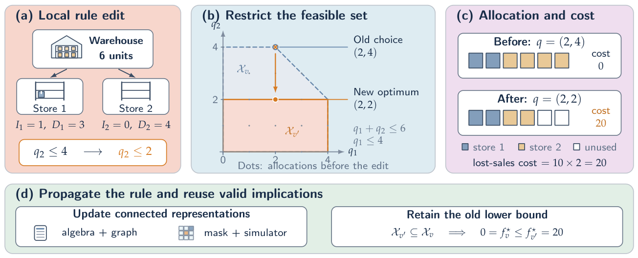
Training examples should include such linked edits. Entity renaming and consistent changes of units preserve the mapped optimization problem; a capacity change alters it. The learning target is therefore both invariance to changes of description and sensitivity to changes of mechanism. Equivalent problems may have several optimal solutions, so evaluation compares feasibility and value after mapping rather than a solver’s arbitrary tie-breaking choice.
5.2. Record What Generated the Observation
A sequential decision record can be written as
where is the current decision specification; the three action fields distinguish proposal, approval, and execution; links subsequent observations; records the candidate set, question or rubric, scores, and any reported confidence; records checks; and records source, model, rule, and event versions. Each event has its own timestamp. Observed, inferred, simulated, and unavailable quantities are identified separately.
For a structured judgment interface, retain the exact question, option order, rubric levels, returned distribution, and model version. Record any masks, thresholds, or OR computations applied after scoring. A question’s judging criteria are not the same object as an approved operational rule: a prompt edit must not silently change a capacity or service obligation.
This organization has a statistical purpose. A lead-time label is attached to the dispatched order and its realized receipt. A sales label is attached to available stock. A policy-learning sample describes the action actually taken, including an override. The observation process then determines the likelihood or learning objective, rather than being treated as a preprocessing detail [56].
- A censored-demand likelihood.
For conditionally exogenous integer demand , let availability be known before demand and sales be . Let be the conditional demand mass function using pre-demand information. Conditional on availability, the negative log-likelihood of sales is
A stock-exhausting sale is a tail observation, including the equality case . Treating it as exact demand trains a different statistical model. Here the observation mechanism determines the statistical objective. Inventory-learning research develops the associated estimation and exploration problems [73,74].
5.3. Four Complementary Training Signals
- Structural alignment.
Paired text, algebra, graphs, and executable models teach correspondences among entities and constraints. Synthetic instances and back-translation expand coverage [8,9]; rule edits and near-boundary examples make the distinctions consequential. Training and evaluation splits separate templates, generators, and constraint compositions.
- Decision supervision.
OR-generated actions provide labels containing the effect of costs, constraints, and time coupling. When supervising a score, distinguish event labels, rubric judgments, pairwise preferences, and realized or simulated decision costs. Business-value targets carry units and a horizon; ordinal ratings do not acquire those properties merely by averaging their levels. Probability targets can use proper scoring rules, while action selection is tested by decision loss [24]. Decision-focused losses in Equation (12) provide a second route when optimization can participate in training. Label provenance includes the information used by the reference solver, its solution quality, and its time limit. Future realizations used to construct hindsight labels remain outside the deployed model’s inputs.
- Search and feasibility feedback.
Incumbents, bounds, violated constraints, repair trajectories, and solver traces teach which candidates and computations are useful [6,12]. An irreducible infeasible subsystem localizes a conflict in a formulation; selecting a business requirement to relax requires its declared priority or owner. Keeping these two labels separate lets a model learn diagnosis without learning arbitrary rule changes.
- Operational response.
Executed trajectories update demand, delay, and policy-value estimates under the relevant observation model. Known accounting structure can remain fixed while these empirical components adapt. Model updates are evaluated under the distribution induced by the policy, since actions can change both outcomes and future training data [80]. A chosen supplier’s outcome does not reveal the outcomes of rejected suppliers. Off-policy comparisons therefore require suitable support and identification assumptions, not just a log of model scores [56]. A Choice distribution is not the behavior policy’s action propensity unless the system actually samples actions from that distribution. Log the implemented selection and exploration rule, including deterministic OR selection and human overrides.
These signals need not be summed into one loss. A formulation model, a demand model, and a branching policy have different targets. What they share is the record format: each training example must identify the specification, computation, and outcome it came from.
5.4. Learn Sufficient Structure for the Intended Decisions
The desired abstraction retains information needed for admissibility and comparison. A state containing only total stock may omit its location or in-transit composition. A demand mean may omit the tail needed for a service constraint. Value-aware and value-equivalent learning formalize the dependence of a model on its planning queries [60,61]. The bound in Equation (17) further separates the cost of omitted choices from distorted values and incomplete search.
For a compressed history , a decoder using only z can remain admissible for every represented history by choosing from
This permits conservative compression, whose opportunity cost is measured by . If the intersection is empty, the decision interface needs more information or a different representation. By contrast, information absent from the original observations cannot be restored by an encoder. For example, logs with availability at most three cannot distinguish constant demand of three from constant demand of five. Appendix A.6 quantifies the resulting decision ambiguity.
Mechanism-conditioned pretraining should consequently cover variations in network structure, objectives, constraint combinations, observation processes, and response regimes. Correct, incomplete, and misspecified mechanisms are separate experimental conditions. They test whether the system gains from structure and whether it can localize the component that needs revision. Reusable learning therefore needs both task diversity and records that preserve decision meaning. The runtime architecture must carry those same records through computation, commitment, and execution.
6. Agent Architecture: Score, Compute, Commit, and Learn
6.1. Assemble a Decision-Specific Computation
An OR-native agent assembles reusable components around the current decision specification and information state. It chooses what to retrieve, which model to construct, which candidates to evaluate, and when to commit to an action. Figure 4 connects these choices to analytical tools and operational records. A static task may use formulation and constrained search; a sequential task adds state estimation, response modeling, and replanning.
Figure 4.
Proposed agent architecture. A typed judgment adapter connects a structured judgment model (for example, Jev) or another learned estimator to OR and numerical tools. Reusable learned components and the current decision specification remain separate inputs. Checks establish local acceptability, the commitment boundary controls execution, and actual actions and outcomes update the next decision record.
Figure 4.
Proposed agent architecture. A typed judgment adapter connects a structured judgment model (for example, Jev) or another learned estimator to OR and numerical tools. Reusable learned components and the current decision specification remain separate inputs. Checks establish local acceptability, the commitment boundary controls execution, and actual actions and outcomes update the next decision record.
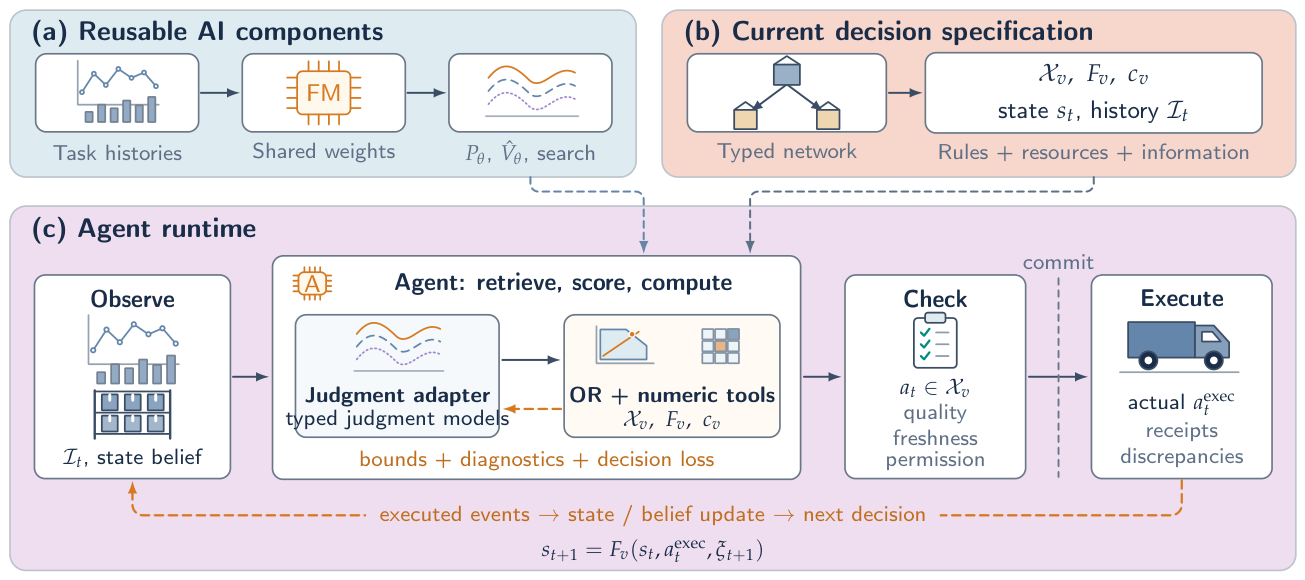
The division of labor follows the stability and mathematical role of each component. Weights reuse formulation patterns, response priors, value estimates, and search strategies. Retrieval supplies current rules and local data. Optimizers apply the feasible set and objective. Simulators compose uncertain inputs with structural updates. The agent selects and connects these operations. An explicit world model is useful when action-conditioned response must be predicted; it is unnecessary for a fully specified static allocation.
This division of labor yields three common execution patterns. A direct policy produces candidates that pass through constrained decoding or validation. A model-guided optimizer uses learned coefficients, warm starts, decompositions, or branching decisions. A scenario-based planner evaluates nonanticipative policies using learned uncertainty and explicit dynamics. In each case, the learned component supplies a different part of the computation, so its contribution is measured by replacing that component while holding the rest of the interface fixed.
6.2. Give Structured Judgment Models an Explicit Boundary
A structured judgment model, such as Jev (Section 4.5), can be integrated through a narrow adapter: retrieve the relevant authorized state, pose a bounded question with an explicit rubric, and return a typed judgment to the planner. The adapter records the response without interpreting confidence as permission to execute. A conventional classifier or another structured model can implement the same role, allowing its contribution to be tested without changing the rest of the planner.
For a small complete candidate set, code may first reject inadmissible actions, then use a validated value model to rank those remaining. For a large combinatorial problem, enumerating all actions is usually impractical. Learned scores may instead guide branching, partial-plan expansion, or candidate screening inside a structured optimizer. Screening changes the retained class and must be assessed through in Equation (17); exact optimization of a screened subset is not a global optimality claim.
In the disruption example of Section 3.1, a judgment such as “supplier delay is likely” can trigger retrieval of shipment evidence. Expediting still requires a validated risk estimate, an action-effect model, costs, and current capacity. A low score, an ambiguous rule, or a weakly supported prediction can instead trigger clarification or fallback. These routes are selected by expected consequences and authority, not by a universal confidence threshold. Exact arithmetic, date comparison, and discrete feasibility stay in code or solvers, consistent with documented limitations of current judgment models [3].
6.3. Choose between Computation and Information Acquisition
Let h record the current information, evaluated candidates, checks, and remaining resources. Let contain the currently available, checked actions, including a specified fallback. Define
where u is a prospective meta-action and its resulting history. Because is computed only over actions already generated and checked, it can fall when the agent does more work: search can add a better candidate, a data query can change estimated consequences, and clarification can resolve which constraints apply. Their net values include computation, delay, and human effort [81,82].
A policy over these meta-actions can be evaluated by
where is the terminal action or fallback and all costs use compatible units. Approximate value estimates can guide orchestration, while fixed workflows and simple stopping rules provide comparisons.
- A value-of-clarification calculation.
In the future-epoch allocation of Section 7.6, suppose the active store-2 cap is two or four with equal probability. Until it is resolved, require feasibility under either value. The best common allocation is , with cost 20. Immediate clarification permits under the lower cap and under the higher cap, with expected cost . With a query cost of two, Equation (29) gives , so asking first is worth eight units. Further optimization of the already solved common feasible problem leaves its cost at 20. The calculation identifies a situation in which information, rather than search, is the useful next input.
6.4. Maintain Local Applicability and Reuse Valid Computations
Before a model output becomes an operational decision, it must pass the five checks in Table 4. Each answers a different question, so passing one does not imply passing another.
Mechanism changes need not invalidate every computational artifact. Tightening a feasible set preserves an old lower bound for the same minimization objective, although it may invalidate the old incumbent. Relaxation preserves the incumbent but may invalidate the bound. Appendix A.8 gives these conditions. An agent can therefore reuse evidence by tracking the mathematical dependencies of each artifact, reducing repeated computation after local edits.
For shared stock, validation and reservation belong to one concurrency-controlled commitment procedure. Stable action identifiers make retries distinguishable from new orders. Execution records then identify what was dispatched, received, and sold. These interfaces connect a feasible recommendation to the state that will actually be used in the next computation.
6.5. Update the Component That Changed
A stock correction updates state; a cap change updates the feasible set; a lead-time shift updates an empirical response model; and a partial dispatch updates the execution record. These events call for different computations. Keeping their histories separate lets an agent adapt locally while retaining unaffected learned and symbolic components.
Interactions with independent suppliers, carriers, and stores additionally involve their objectives and responses. Requests, offers, commitments, and executed actions are distinct events. Policy changes can alter the empirical relationships learned from past behavior [80,83]. Replanning therefore combines updated observations with the outstanding commitments that still constrain the system. The loop closes when execution and its consequences update the next decision record. The following cases show where these interfaces enter operational systems.
7. Supply-Chain Cases and Worked Decisions
Coupled material flows, uncertain demand, and delayed execution make supply chains a demanding setting for the proposed interfaces. The JD.com systems below connect learning and operational mechanisms in different ways. For each, we ask what is learned, what is specified, and how feedback enters the computation. The evidence ranges from offline and production-batch evaluations to deployed systems and field comparisons.
Several of our authors contributed to these studies; their results are cited, not replicated here. Mapping them onto the interfaces of this perspective is our interpretation: the systems were not built under the ScoAI name and do not use a structured judgment model.
7.1. A Portfolio of Computational Interfaces
Table 5.
Learning and operational mechanisms in the JD.com portfolio. Different settings and study designs are reported separately.
Table 5.
Learning and operational mechanisms in the JD.com portfolio. Different settings and study designs are reported separately.
| System | Data / learned component | Operational mechanism | Setting / evidence |
|---|---|---|---|
| Warehouse robots [84] | Live task, robot, rack, and workstation state | Integer optimization and decomposition coordinate dispatch within operating deadlines | Production warehouses |
| End-to-end inventory [85] | Features mapped to replenishment quantities | Dynamic-programming decisions supervise a neural policy | Real-data experiments and field comparison |
| Assortment and allocation [86] | Demand forecasts and inventory policies | Assortment, allocation, and simulation connect learning to fulfillment and inventory costs | Out-of-sample tests; deployed support across eight RDCs |
| ORPR [17] | Pretrained replenishment policy with subsequent reinforcement | Simulation-augmented OR labels and expert-guided refinement | One-month field comparison with DiD analysis |
| Generative planning [16] | Semantic interpretation and task decomposition | Data and analytical tools execute a context-dependent planning workflow | Deployment; year-over-year operational comparison |
| ORLA [77] | Formulation generation and learned quality estimation | Solver feedback supports training, formulation selection, and aggregation | 29 production batches; five unseen task categories |
| SCOPE [78] | Shared representations and conditional policies | Stage-specific training and full-pipeline validation coordinate decisions | Offline evaluation with dataset-specific checkpoints |
The warehouse-robot system demonstrates the operational structure that a learned interface must preserve. It coordinates robots, racks, and workstations through integer optimization and fast decomposition under real-time deadlines [84]. Current state, shared resources, and dispatch timing are inputs to the computation. Reusable learning can contribute to modeling or search while keeping that execution structure explicit.
7.2. Inventory: OR Supplies Supervision and Learning Supplies Adaptation
The end-to-end inventory model learns replenishment quantities from operational features using decisions from dynamic programming as training guidance. Its labels encode multi-period consequences of demand and vendor lead times [85]. ORPR extends the training interface through simulation-augmented OR reference decisions, pretraining, reinforcement learning, and expert-guided refinement [17].
Using notation introduced here, the shared computational pattern is
The reference decision carries the objective, constraints, and intertemporal tradeoffs into supervision. Subsequent decision-cost refinement adapts the policy to the modeled operating environment. These equations summarize the interface, rather than reproduce either paper’s training algorithm. They identify two contributions to test separately: the quality of OR supervision and the benefit of adaptation after pretraining.
ORPR’s field comparison ran from September 1 to October 1, 2025, covering 331 SKUs and 3,899 SKU–distribution-center pairs. The study reports a 5.27-day reduction in turnover, an in-stock-rate gain reported as 2.29%, and a 29.95% reduction in holding cost, accompanied by a difference-in-differences analysis [17]. The relevant fusion lesson is that structured decisions can serve as a learning resource and initial policy, with operational refinement targeting the remaining mismatch. The reported effects concern the combined inventory system.
7.3. Assortment and Allocation: Couple Forecasts Through Shared Resources
The regional distribution center (RDC)–front distribution center (FDC) system combines assortment selection with inventory allocation and uses a forecast–optimize–simulate learning pipeline [86]. Its mechanism connects which products are available locally to how regional stock and front-warehouse capacity are used. For a simplified single-RDC slice, let indicate assortment of product i at FDC j, and let be allocated units. The coupling includes
where is regional stock, unit storage volume, FDC capacity, and an allocation bound. Demand estimates determine the value of an allocation, while assortment and capacity determine whether it is available. Simulation feedback exposes the resulting fulfillment, transfer, shortage, and inventory costs to learning.
The study reports out-of-sample gains of 0.54 percentage points in local order fulfillment for assortment and 1.05 percentage points in FDC demand fulfillment for its allocation comparison, together with deployed decision support across eight RDCs [86]. The mechanism in Equation (33) explains why demand accuracy alone is an incomplete training target: the value of an error depends on shared stock, assortment, and the capacities binding elsewhere in the network.
7.4. Planning and Formulation: Learn How to Construct the Computation
The generative planning system connects business requests with data acquisition, analysis, and inventory planning tools. The report describes deployment from December 2023 and evaluates more than 70,000 SKUs across three business units. For the May–June 2024 promotional period relative to the corresponding 2023 manual baseline, it reports a 22% increase in the share of plans with inventory-value deviation below 5% [16]. Its fusion interface is semantic and computational: the learned component interprets context and assembles the analytical workflow used to make a plan. The outcome comparison is year-over-year.
ORLA moves the learned interface into optimization-model construction and selection. It generates formulation candidates and code, uses solver feedback in post-training, estimates candidate quality, and combines selected outputs [77]. The business objective includes balance in target inventory days. For warehouse k with current inventory , allocation , and positive forecast daily demand , the post-allocation coverage is
This ratio connects a statistical forecast to an operational allocation criterion. Its constraints encode quantity domains and scenario-specific requirements, which solver feedback makes available to the learning loop.
Across 29 production evaluation batches, ORLA reports a 4.5-percentage-point overall improvement in its TID-based allocation-accuracy measure. In five unseen task categories, all generated programs execute syntactically and three produce allocations satisfying the tested hard constraints [77]. This separates the learned ability to generate executable code from the ability to reconstruct the complete decision mechanism.
7.5. Coupled Policies: Learn the Value of Downstream Consequences
SCOPE connects assortment, source assignment, replenishment cycles, and routing through shared operational representations and policies conditioned on preceding decisions [78]. This is the cross-stage fusion interface in Equation (18): an upstream choice changes the feasible downstream problem and hence the value of the full plan.
The implementation trains stage-specific surrogate objectives and selects policy checkpoints using complete-pipeline validation utility. Completion value provides a conceptual coordination target here; it is not computed exactly during training. Its experiments use JD.com and public fresh-retail data with separate dataset-specific checkpoints [78]. The case therefore supports an architectural pattern: shared context and explicit handoffs can combine local learning with system-level evaluation. Estimating completion values or capacity prices more directly is a further research question suggested by Equation (19).
Together, the portfolio shows four forms of fusion: OR decisions as supervision, operational cost as a learning signal, solvers as feedback on formulations, and downstream consequences as a coordination target. The first three mainly address the gap between judgment and action; the last addresses the gap between local and system value. The field and production studies also illustrate the third gap, since their reported effects are measured on executed decisions rather than on recommendations. A reusable foundation model could learn these structures across tasks, and an agent could assemble them around the decision at hand.
A structured judgment model would add one more testable interface to this portfolio, not replace it. It could classify a supplier exception, rate the relevance of a retrieved rule, or compare bounded candidate plans. The prediction would still enter the inventory, allocation, or coordination computation under an explicit meaning. The worked example below uses constructed inputs to isolate that connection; it contains no model-generated values.
7.6. A Worked Inventory System
The following constructed example makes the data and mechanism roles explicit. One warehouse ships a single product to stores over periods . Quantities are nonnegative and use one common unit; returns, spoilage, and transit losses are excluded. At each period’s start, due receipts are recorded and dispatches chosen before store demand is observed. Dispatch lead times are positive integers.
- Exact flow, learned uncertainty.
Let be warehouse stock before supplier receipt , and the units actually dispatched. The warehouse relation is
With initial pipeline receipts , realized store arrivals are
Lead times in this ledger are realized transit times. Their distributions can be learned at dispatch, while actual receipts update the ledger when observed. With pre-arrival store stock and latent demand ,
Sales are observed, while lost demand may be unobserved. These equations are the mechanism; the conditional law of demand and transit time is the learned input. They compose into the policy objective
with unit holding, lost-sales, and dispatch costs , subject to the flow relations, dispatch domains, and specified service requirements. A forecast update changes ; a cap update changes ; an executed shipment changes the next state. Each has a distinct place in the same computation.
- Data support determines what can be learned.
In this system, the censoring example of Section 3.7 arises directly: if store availability has never exceeded three, constant demands of three and five leave identical sales logs, and no stocking rule based on those logs avoids a regret of at least one in both (Appendix A.6). Stocking four units in one period separates them, since sales would be three or four. The censored likelihood in Equation (27) uses such an observation correctly, and the choice to stock four becomes an information-acquisition decision whose cost can be weighed against its value.
- Service requires the relevant distributional information.
For nonnegative demand with , cycle service and volume fill rate at stock z are
If demand is zero with probability and 100 with probability , stock three gives 99% cycle service but 3% volume fill. Mean demand is one, as for constant demand one, which the same stock fully serves. Thus the service mechanism determines which aspect of the demand law must be preserved by the learned representation.
- A rule edit changes the optimization problem.
For a deterministic future arrival epoch, let projected pre-arrival store stocks be , demands , and warehouse availability six. With single-unit dispatches, lost-sales cost ten, holding cost one, and zero shipping and warehouse holding costs, solve
For caps , the optimum is with cost zero. Tightening the second cap to two gives optimum with cost 20 and leaves two units at the warehouse. This is the edit shown in Figure 3. It changes the admissible action and optimal value without changing the demand assumption or requiring a new representation of inventory conservation. Even if a score model continues to favor the old plan, the updated OR model rejects it. Among admissible candidates, decision cost rather than model confidence selects the plan: a model may judge an alternative, but only the constrained computation can certify it as a valid operational decision.
A domain edit has a different effect. In the instance above, the optimum already consists of even quantities, so two-unit case packs would not bind. Consider instead empty stores, , demands , the same six units, caps , and costs. Unit dispatches give the optimum with cost zero. Two-unit case packs, with , make inadmissible; rounding both entries up to violates the six-unit limit. The admissible optima are and , each with cost . If both stores must receive at least three units, the packed problem is infeasible. The coupled domain must therefore be applied before an action is released, and rounding a unit solution is not a substitute for solving the packed problem.
- Execution supplies the next training and decision record.
An approved dispatch may be executed as . Figure 5 records that difference, the delayed receipts, and the subsequent censored sales. The state update uses the executed quantities, and learning uses the observations linked to them. An accurate proposal alone would not determine this update: executed quantities establish the state, and the observation mechanism determines what the resulting sales reveal.
The example permits controlled comparisons of prediction models, two-stage forecasting and optimization, mechanism-informed training, and structured planning. Each policy generates its own stock availability and observation history. Rule, demand, service, domain, and lead-time changes then test different parts of the interface, using the metrics developed next.
8. Evaluation: Judgments, Decisions, and Executed Outcomes
Evaluation should identify which interface improves the decision and at what cost. Compare quality and total cost at matched validity, information, and task coverage. Then isolate representation, learning, constrained computation, and operational updates. The terms in Equations (10) and (17) provide separate diagnostic targets for these comparisons. The protocol for structured judgment models (Section 8.2) covers the first and third gaps; the coordination tests (Section 8.5) cover the second.
8.1. Compare the Interfaces, Not Only the Final Systems
Use the same task data and requirements to compare a specialist OR workflow, a reusable predictor feeding the same optimizer, a version trained with decision or mechanistic feedback, and an agent that selects its computations. This sequence separates predictor reuse, training feedback, and orchestration. A direct learned policy provides an additional proposal baseline where relevant; strong specialist policies remain essential comparators.
The ablations hold solver access, data cutoffs, hardware, and total budgets fixed. Replacing prediction-only training with decision loss isolates the training interface. Replacing an unrestricted transition with the structured update in Equation (9) isolates the dynamics interface. Removing shared context or downstream feedback isolates coordination. Replacing a pretrained component with a task-specific model measures reuse. Every configuration uses the same independent final assessment; raw proposal feasibility, repair cost, and final validity are recorded separately.
Data size and mechanism quality are additional experimental axes. Vary sample size under correct, incomplete, and misspecified structural assumptions. Measure both statistical risk and induced decision cost. This tests the tradeoff in Equation (10): a smaller hypothesis class can need fewer samples, while an incorrect restriction can impose persistent bias. In sequential tasks, each policy’s actions generate its own observations; historical sales are not replayed as uncensored demand for every policy.
8.2. A Three-Level Protocol for Structured Judgment Models
The protocol has three levels. Judgment quality tests the score against its own declared target. Decision quality tests the conversion of that score into an admissible action, which is the first gap. Operational quality tests what happens once the action is committed and executed, which is the third.
- Judgment quality.
Freeze the model identifier, question, rubric, candidate construction, and information cutoff. For defined binary or categorical events, measure proper scoring losses and calibration on held-out outcomes; report subgroup and shifted-regime results [23,24]. For rubric ratings, assess agreement with the declared rubric separately from business utility. A reported confidence value, a maximum option probability, and an empirically calibrated error probability are distinct quantities. Reorder equivalent options, rename entities, and vary irrelevant context to test stability without silently changing the task.
- Decision quality.
Compare four configurations: offline score-only selection; scored candidates with a separate feasibility check; the scores inside a coupled optimizer; and a strong specialist OR baseline. Include an alternative estimator with the same OR backend to isolate the scoring model. Keep candidate and computational budgets explicit. Report raw proposal violations, post-check coverage, repair costs, and regret under the actual costs and service requirements. Use the three terms in Equation (17) to distinguish missing candidates, value distortion, and incomplete search. A correct discrete answer or a well-calibrated probability is not by itself a successful decision.
- Operational quality.
Compare confidence-gated escalation with cost-sensitive thresholds and fixed workflows. Report human effort, rejected tasks, fallback outcomes, and end-to-end latency, including data retrieval, optimization, and commitment. A candidate model call’s speed is only one component of that latency. Any supply-chain gain requires simulation or operational evidence under the stated design. Version-specific stress cases include numerical and date boundaries, option ordering, and adversarial text in retrieved state [3].
8.3. Test Changes with a Specified Expected Response
A test instance includes the original decision specification, the edit, and the expected effect on the computation. Entity renaming or consistent unit conversion preserves the mapped feasible problem. Capacity, case-pack, and precedence edits change admissibility. Cost and service edits change action ranking. Demand or lead-time shifts change empirical response. An observation change alters what can be inferred.
Hold out constraint combinations, network sizes and topologies, objective weights, service definitions, and observation regimes. Include near-binding resources and infeasible combinations. Separate template families and data generators across training and test sets. For equivalent edits, compare mapped feasible sets and objective values rather than exact optimizer vectors (Appendix A.9). For changed requirements, measure whether all relevant representations and computations respond.
A transfer report identifies the reused checkpoint, parameter updates, retrieved context, demonstrations, search calls, and task-specific engineering. A fixed checkpoint with in-context examples and a fine-tuned checkpoint are reported as different protocols. Benchmark revisions and corrected labels likewise define separate evaluation versions; OptiMind and OptMATH illustrate why annotation and scoring conventions matter [9,44].
8.4. Measure Quality, Validity, Coverage, and Cost Jointly
For M attempted tasks, let indicate an accepted output and a detected hard-obligation violation in that output. Report
These are the empirical counterparts of and in Equation (23). When no output is accepted, conditional violation and quality rates are unavailable, while coverage is zero. Report cost per attempted task, cost per accepted output when defined, and the operational consequences of fallback. Quality includes objective value or regret, tail loss, service, and completion feasibility. Validity includes physical-unit residuals, discrete violations, deadline misses, and current-rule consistency.
Uncertainty accompanies each estimate. For example, with independent identically distributed accepted decisions and zero observed violations, the one-sided binomial upper confidence bound is
This follows from . Repeated product, facility, or temporal observations generally require a clustered or dependence-aware analysis instead. Stratified results expose systematic abstention or service failures hidden by an overall average.
The total-cost accounting in Equation (22) includes pretraining, adaptation, specification, tool calls, retries, verification, human queries, and delay. Show fixed costs separately and use plausible amortization volumes. Report the frontier when no system dominates across validity, quality, coverage, latency, and cost.
8.5. Separate Value Approximation from Coordination
On tractable instances, evaluate the full feasible reference class, the retained candidate class, their true costs, and the learned cost estimates. This gives restriction loss , relative-value distortion , and planning error separately. For large instances, use justified bounds or strong reference policies, and report the remaining uncertainty. A perfect-future-information policy is a separate bound rather than a like-for-like deployed competitor.
For a coupled pipeline, compare independent modules, explicit handoff features, shared representations, and completion-value or system-utility feedback. Vary coupling strength through shared capacity, lead times, and service requirements while holding local prediction difficulty as stable as possible. For each partial plan, assess downstream completion under the same information and computational limits. Report end-to-end cost, frequency of no feasible completion, repair burden, and upstream decisions that cause downstream congestion. This tests the coordination mechanism in Equations (18) and (19).
8.6. Match the Evidence to the Outcome
For a minimization problem, a valid lower bound ℓ and feasible incumbent value u establish for the stated model. Model fidelity and execution use the other evidence in Table 6. A learned feasibility classifier is evaluated against an independent checker, and a generated repair is re-evaluated under the current requirements.
Retrospective replay, simulation, shadow use, planner-approved pilots, and controlled deployment answer different empirical questions. Shadow use measures availability, timing, and proposal quality; executing a policy makes its operational outcomes observable. Intervention comparisons specify assignment, exposure, outcome windows, overrides, missingness, support, and interference [87]. The JD.com cases retain their individual study designs and metric definitions. Their evidence identifies interfaces worth testing; controlled ablations are needed to attribute a gain to a particular component. The resulting research agenda concerns which interface changes improve decisions, under which task shifts, and at what cost.
9. Research Priorities
The preceding analysis suggests six research priorities. Each concerns a specific interface and can be tested against a simpler alternative. Together they ask what should be learned, how it should transfer, and when the added computation pays for itself.
9.1. Learn Decision-Relevant Scores, Not a Universal Rating
Structured judgment interfaces (Section 4.5) make the learning target explicit. The research question is which targets improve operational decisions: event probabilities, rubric ratings, action values, or completion values. A scalar used across tasks must specify the objective, horizon, units, and uncertainty it represents.
Compare generic rubric scoring, calibrated event prediction, and cost-conditioned value learning with the same candidate set and OR backend. Vary loss asymmetry, tail risk, and resource coupling separately. The hypothesis is that decision-conditioned scores reduce , but only where the retained candidates and available information can support a good action. Evaluate calibration under policy-induced shift and include score abstention or clarification in the cost comparison. The test is whether each target preserves the distinctions needed by the intended decision family.
9.2. Mechanism-conditioned Representations and Constraint Composition
A supply-chain foundation model should condition its predictions and proposals on the mechanism of the task: entities, network edges, resource constraints, objectives, and observation rules. This allows pretrained structure to be reused when coefficients or combinations change. MVMoE and MILP-Evolve provide starting points for studying this form of transfer [13,14].
The hypothesis is that structural diversity in pretraining improves adaptation to new constraint compositions more than additional paraphrases of a fixed formulation family. Test it by holding out combinations, topology–constraint interactions, case-pack domains, and cost or service changes. Compare a generic model with equivalent tools, a specialist model, and a mechanism-conditioned model at matched adaptation budgets. Measure feasibility, decision loss, and sample requirements. Structural coverage then becomes a meaningful dimension of scale alongside model and dataset size.
9.3. Optimization Feedback as a Reusable Learning Resource
Solutions, valid bounds, conflict sets, repair traces, and near-boundary counterexamples contain more decision information than final answers alone. Training should connect each artifact to the specification that produced it. This supports learning both how to propose a decision and how to revise it when a mechanism changes.
Two hypotheses follow. First, diverse solver and mechanism feedback should improve error localization and transfer beyond the training generator. Second, dependency-aware reuse should reduce the amount of checking required after a local edit. Compare solution-only training with richer feedback using an independent test checker. Compare complete recomputation with selective reuse under the conditions in Appendix A.8. The measurements are proposal validity, repair effort, retained-bound quality, and total computation. This direction treats optimization outputs as training data with mathematical meaning and usable provenance.
9.4. Goal-aware Abstraction and Cross-Stage Coordination
Reusable representations should retain the structure needed by several related objectives, horizons, and service requirements. The learning target is not full reconstruction of every detail, but useful feasible choices and adequate value comparisons across the intended query family [60,61]. The terms in Equation (17) specify what to measure as the representation is compressed or the goal changes.
For supply chains, this abstraction must also carry downstream consequences. Completion values and resource prices offer two possible interfaces. A model may estimate how an assortment changes attainable fulfillment cost, or how an extra unit of warehouse capacity changes network value. These quantities can coordinate specialized policies without forcing every stage into one output sequence. SCOPE’s shared representations and full-pipeline validation motivate this direction; direct completion-value estimation and price-based coordination remain distinct targets to investigate [78].
Compare independent policies, explicit handoffs, shared context, and learned completion or price signals under increasing coupling. The expected benefit should grow where capacity and timing externalities are substantial. Evaluate complete plans and the cost of producing those coordination signals.
9.5. Allocate Reasoning, Checking, and Information Budgets
An agent chooses the computation as well as the operational action. The next useful step depends on whether the limitation is a missing candidate, an uncertain value comparison, an unresolved rule, or an unobserved quantity. Metareasoning supplies the decision-theoretic basis [82]; the fusion interface makes these states explicit to the orchestrator.
Construct matched tasks in which further search, an informative query, or an authorized change to the action set is the useful intervention. Vary tool prices and deadlines, and compare learned orchestration with fixed workflows, simple thresholds, and budget rules. Charge for the information and computation used to learn the orchestrator as well as its runtime calls. Agent scaling studies [64] can then be extended from prediction or return to the supported-decision frontier.
This also gives a direct test of foundation-model economics. Measure fixed investment and recurring cost across task volume and mechanism-update rates, and compare the observed crossover with Equation (24). A specialized optimizer may remain the lower-cost choice for a narrow stable task; reusable models are most useful when the same investment serves many related decisions.
9.6. Adapt Data and Mechanisms at Their Respective Time Scales
Demand patterns, transit delays, inventory state, and operating rules change at different rates. A fused system can update a demand estimator, refresh a state ledger, revise a constraint, or retrain a policy independently when the interfaces remain consistent. This suggests a two-level design: reusable representations and computational skills across tasks, with local state and mechanism versions supplied at decision time.
Test selective adaptation against periodic full retraining and retrieval-only updates under isolated and combined changes. Censoring and delayed execution are especially useful tests because they determine when new information becomes available. Evaluate whether the system updates the affected component, retains valid computations, and attributes outcomes to the executed action.
The same logic applies to deployment-driven data collection. An action can improve both immediate performance and future knowledge, as in the inventory observation example. Learning should therefore account for which observations the policy makes available and the operational cost of acquiring them. This connects model adaptation, experimental design, and OR planning within one computational objective.
These priorities share one experimental discipline: change a defined interface, hold the comparison conditions fixed, and measure the effect on decisions. Progress means a better quality, validity, coverage, and cost frontier across related tasks, with the effort required for transfer included in the comparison.
10. Conclusion
The useful output of a foundation-model workflow is a decision whose meaning, feasibility, and consequences can be assessed. This perspective has organized that requirement around explicit interfaces: scores are connected to costs, candidates to constraints, local choices to downstream value, and proposed actions to execution records. Data–mechanism fusion makes those connections available to both learning and computation.
Each of the three gaps has a distinct remedy. Between judgment and action, consequence costs give scores a decision meaning; structural knowledge reduces estimation demands when its assumptions are valid, decision-aware learning improves value comparisons, and constrained computation preserves admissibility. Between local quality and system value, completion values and resource prices coordinate stages. Between plan and execution, records of approved and executed actions determine the next state and what the resulting observations can reveal. None of these substitutes for candidate coverage or for evidence from execution. Structured judgment models are one promising source of learned components; the proposed adapter and evaluation protocol specify how their operational contribution would be tested.
The JD.com cases and constructed examples serve different purposes: the former illustrate reported systems, and the latter make the decision logic reproducible. Together they motivate a research program measured by quality, validity, coverage, and total cost rather than by confidence or generation quality alone.
ScoAI = SC + OR + AI captures this program in one organizing idea: learn reusable judgments, compute under explicit mechanisms, and improve through the consequences of executed decisions.
Appendix A. Mathematical Details and Worked Checks
This appendix gives the assumptions, proofs, and constructed calculations supporting the decision interfaces in the main text. The calculations check the argument; they do not estimate industrial or hosted-model performance.
Appendix A.1. Probability Thresholds and the Meaning of an Average Score
For the disruption example in Equation (8), let denote expediting and no action. The expected cost is
Either action is optimal at equality; the displayed policy chooses no action. For an estimate , the induced regret satisfies
If the actions differ, p and lie on opposite sides of the threshold (allowing equality), so the distance from p to the threshold is at most . Otherwise regret is zero. At , acting on costs 10 instead of 6: regret 4 is below the bound 5. This bound concerns a probability of the defined event; it does not apply to an arbitrary confidence score.
An average rubric score can discard information needed by the decision. Consider three levels , with distributions and . Both have average level 1. If the corresponding consequence costs are , their expected costs are 50 and 1. Consequently, a shared mean rating does not imply a shared operational value. The level distribution and consequence map, or a directly validated value estimate, are needed. This is distinct from numeric precision: even exact arithmetic on the average cannot recover the discarded information.
Appendix A.2. Estimation Under a Fixed Structural Restriction
Let be independent identically distributed samples, , and let the nonempty finite class be fixed independently of these samples. For loss , define
For and , Hoeffding’s inequality and a union bound give
Choose , so the right-hand side equals . On the complementary event, which has probability at least , take a population minimizer over the finite class; then
Subtracting the reference risk and writing yields Equation (10). To make the estimation term at most , it suffices that
Thus a fixed valid restriction reduces this sufficient sample bound through class size. A restriction estimated from the same data requires its own complexity control or an independent fitting sample. Serially dependent operational data and neural hypothesis classes require corresponding concentration and capacity analyses. The approximation-bias term remains explicit in each case.
Appendix A.3. Information, Policies, and Structural Transitions
Let denote latent state and an observation. A sequential model specifies
The state includes variables needed by the assumed dynamics, such as outstanding shipments and relevant regimes. The information record contains observations released by the cutoff, past executed actions, and the rules disclosed by that time. Set . An admissible policy is nonanticipative: its action is measurable with respect to , augmented by permitted randomization independent of future shocks. A belief is one possible information state [36,38].
In Equation (9), the learned generator supplies uncertain inputs in valid domains and the known map applies the accounting update. This composition defines a valid transition law when the generator and map are measurable and their domains match. Positive integer transit times and nonnegative demand can be enforced at the generator interface.
The actor’s information set matters. A human override based on private information is an execution channel beyond the agent’s policy. Outcome models condition on the executed action and the relevant information, while evaluation keeps the agent’s original information cutoff. Robust and chance constraints then use their declared support or probability semantics [35,37,66].
Appendix A.4. A Feasibility Margin with Separate Error Sources
Consider continuous inequalities . Let be the modeled constraint, x the nominal decision, and its executed realization.
Proposition A1
(Inequality protection). Suppose nonnegative satisfy
If for each row, then for each row.
Proof.
For every i,
□
The error bounds hold at the selected and executed points. For a linear row, can be the dual norm of its coefficient vector. All terms use the same residual units. If the premises hold on a joint event of probability , the conclusion holds on that event. Integer domains and exact flow equalities use their corresponding discrete and structural checks.
Appendix A.5. Proof of the Decision-Loss Decomposition
For Proposition 1, both J and are real-valued on , their required infima are finite, and . For every , the definition of gives
Taking the infimum over and adding proves Equation (17), without requiring attainment of the true infimum. If each absolute value error is at most , the difference of two errors is at most . □
The decomposition is tight in a finite example. Let admissible actions have costs , but retain only . Give both retained actions learned cost 2 and let the planner choose b. Then , , , and the decision loss is 3. A common offset added to all learned values instead leaves unchanged. These examples distinguish value ranking from absolute prediction accuracy.
The premise handles feasibility separately. If the learned feasible set admits a prohibited action, value accuracy on the true feasible actions does not control selection of that action. Likewise, a reference policy using future information belongs to a different comparison class. The bound is evaluated for the specified feasible policies and information.
For the compressed-history condition in Equation (28), every action decoded from z must be admissible in every history mapped to z; intersecting those admissible sets gives the condition directly. A smaller nonempty intersection permits conservative decisions whose value loss can be assessed. A decoder or checker with additional information uses a richer interface and is evaluated as such.
Appendix A.6. A Censored-Log Decision Ambiguity
Proposition A2
(Censored-log ambiguity). Let in the historical data. The only demand record is , with . Compare constant demand 3 with constant demand 5, under the same public context. Any adaptive stocking policy using only these records and independent internal randomization has the same observation law in both environments. For a future stocking quantity based on these records and cost , the larger of its two expected regrets is at least one.
Proof.
Couple the policy’s randomization across environments. Since , both produce ; induction gives identical histories and subsequent choices. Therefore Q has the same law in both. The informed optimal stocks are 3 and 5 with cost zero, and
The constant choice attains the bound. □
An observed unmet-demand indicator at availability three distinguishes the environments, whereas a stock-exhaustion flag does not. Availability four in a later period also separates them. The result isolates the information contained in the restricted logs and complements adaptive inventory learning under broader exploration protocols [73,74].
Appendix A.7. Optimization Sensitivity and Shared Resource Prices
For the equality-constrained quadratic program in Equation (13), stationarity and feasibility are and . The block matrix is invertible: if and , then , so ; full row rank of A then gives . Differentiating these equations for differentiable proves Equation (13).
As a numerical check, take , , , and . The optimizer and derivative are
A change in one predicted cost moves both decisions because they share a resource equality.
For Equation (19), the dual function at resource vector b is
Under the saddle-point assumption, strong duality gives . The dual function is affine in b for fixed : . Weak duality at , which needs no convexity, then gives
which proves Equation (20). Convexity of and makes convex, so is a subgradient. A plan x is optimal if and only if is a saddle point, that is, x minimizes , satisfies the coupling constraint, and satisfies complementary slackness. For the linear program , the price makes every a local minimizer, although only points with are optimal. For integer models, strong duality can fail; the same dual construction then supplies a lower bound and coordination signals, while primal reconciliation remains necessary.
Appendix A.8. Reuse After a Constraint Edit
Let be nonempty feasible sets for the same objective f, with finite values . Let be an old lower bound and an old incumbent. Set inclusion gives
Tightening preserves the lower bound, and relaxation preserves the incumbent. For , tightening to invalidates incumbent 0; relaxing to invalidates old lower bound 1. In the worked allocation, the tightened cap preserves lower bound zero but changes the optimum to 20. Reuse therefore tracks the objective, feasible-set relation, units, and numerical conventions of each artifact.
Appendix A.9. Equivalent Descriptions Preserve Optimizer Sets
Suppose is a bijection and for every , with . The order-preserving transformation gives
This preserves the solution set rather than a particular tie-breaking choice. Unit conversions transform domains as well as coefficients: integer items become multiples of when measured in dozens. Absolute objective tolerances scale by a, and feasibility tolerances follow the units of each constraint. These are the invariants used in paired semantic tests.
Appendix A.10. Propagation of Transition Error
For deterministic transitions under the same prescribed action sequence, let d be a state metric and assume
Writing , the triangle inequality gives , and hence
This identifies the initial-state and per-step error contributions. For state-feedback policies, the corresponding bound requires closed-loop regularity or explicit action-error terms; stochastic models require a specified coupling or distributional metric. Structured accounting focuses model estimation on uncertain inputs, while long-horizon evaluation still checks how those uncertainties propagate through the chosen policy.
Appendix B. Reporting Requirements and Evidence Scope
Appendix B.1. A Reproducible System Description
- 1.
- Decision: Task family, units, horizon, objective, constraints, and available information.
- 2.
- Data: Observed, inferred, simulated, and missing fields; cutoffs, splits, and action–outcome links.
- 3.
- Mechanisms: Accounting, rules, and response models; their roles in representation, training, inference, and updates.
- 4.
- Scores and learning: Targets, rubrics, candidates and order, distributions, confidence semantics, model versions, calibration data, label quality, reuse and adaptation budgets, and actual action-selection rules.
- 5.
- Computation: Solvers, simulators, candidate generation, repair, stopping rules, and checks.
- 6.
- Coordination: Shared resources, handoffs, and the complete-plan objective.
- 7.
- Evaluation: Quality, validity, coverage, latency, uncertainty, and fixed and recurring costs.
- 8.
- Operation: Permissions, reservations, commitment, execution records, update owners, and fallback.
Identify each capability as tested, source-attributed, or proposed. Record both data and tool access boundaries, including those for cross-organization reuse.
Appendix B.2. Review and Case-Study Scope
This is a representative perspective on data–mechanism interfaces, not a systematic review or meta-analysis. It connects OR and decision learning to scientific and state-transition modeling, including neighboring-domain perspectives [21,88].
Industrial effects retain each source’s metric, study design, period, and unit of analysis. Benchmark, production-batch, offline-data, and field results are distinct. Several authors coauthored the JD.com studies in Section 7; the case evidence is attributed, not independently replicated here.
Jev’s evidence consists of first-party documentation and the September 15, 2026 launch announcement, accessed through October 8, 2026. The limitations concern jev-1.13, with a documentation review date of October 2, 2026 [3]. No hosted-model experiment or training reproduction is reported; adapters and evaluation protocols are proposals. Typed outputs establish an output space, not calibrated truth or operational feasibility.
Proofs state their assumptions. The disruption and inventory examples are constructed reproducibility checks, not industrial effect estimates.
References
- Bommasani, Rishi; Hudson, Drew A; Adeli, Ehsan; Altman, Russ; Arora, Simran; von Arx, Sydney; Bernstein, Michael S; Bohg, Jeannette; Bosselut, Antoine; Brunskill, Emma; et al. On the opportunities and risks of foundation models. arXiv 2021, arXiv:2108.07258. [Google Scholar]
- Yang, Sherry; Nachum, Ofir; Du, Yilun; Wei, Jason; Abbeel, Pieter; Schuurmans, Dale. Foundation models for decision making: Problems, methods, and opportunities. arXiv 2023, arXiv:2303.04129. [Google Scholar]
- TypeSafe, A.I. TypeSafe AI. 2026. Available online: https://typesafe.ai/.
- Liu, Yang; Zhou, Chuan; Chen, Yancheng; Zhang, Shuai; Lin, Xixun; Wang, Xiaoqing. Hard constraints meet soft generation: Guaranteed feasibility for llm-based combinatorial optimization. arXiv 2026a, arXiv:2602.01090. [Google Scholar]
- Bertsimas, Dimitris; Kallus, Nathan. From predictive to prescriptive analytics. Manag. Sci. 2020, 66(3), 1025–1044. [Google Scholar] [CrossRef]
- Elmachtoub, Adam N; Grigas, Paul. Smart “predict, then optimize”. Manag. Sci. 2022, 68(1), 9–26. [Google Scholar] [CrossRef]
- Mandi, Jayanta; Kotary, James; Berden, Senne; Mulamba, Maxime; Bucarey, Victor; Guns, Tias; Fioretto, Ferdinando. Decision-focused learning: Foundations, state of the art, benchmark and future opportunities. J. Artif. Intell. Res. 2024, 80, 1623–1701. [Google Scholar] [CrossRef]
- Huang, Chenyu; Tang, Zhengyang; Hu, Shixi; Jiang, Ruoqing; Zheng, Xin; Ge, Dongdong; Wang, Benyou; Wang, Zizhuo. Orlm: A customizable framework in training large models for automated optimization modeling. Oper. Res. 2025a, 73(6), 2986–3009. [Google Scholar] [CrossRef]
- Lu, Hongliang; Xie, Zhonglin; Wu, Yaoyu; Ren, Can; Chen, Yuxuan; Wen, Zaiwen. Optmath: A scalable bidirectional data synthesis framework for optimization modeling. arXiv 2025, arXiv:2502.11102. [Google Scholar]
- Ao, Ruicheng; Simchi-Levi, David; Wang, Xinshang. Optirepair: Closed-loop diagnosis and repair of supply chain optimization models with llm agents. arXiv 2026, arXiv:2602.19439. [Google Scholar]
- He, Jiayin; Pan, Yutong; Yang, Sen; Kang, Ningxuan; Qi, Yongzhi; Zhang, Jianshen; Qi, Wei; Shen, Zuo-Jun Max. Spord: A simulation-propose-then-or-dispose approach for supply chain planning. arXiv 2026, arXiv:2607.21354. [Google Scholar]
- Gasse, Maxime; Chételat, Didier; Ferroni, Nicola; Charlin, Laurent; Lodi, Andrea. Exact combinatorial optimization with graph convolutional neural networks. Adv. Neural Inf. Process. Syst. 2019, 32. [Google Scholar]
- Zhou, Jianan; Cao, Zhiguang; Wu, Yaoxin; Song, Wen; Ma, Yining; Zhang, Jie; Xu, Chi. Mvmoe: Multi-task vehicle routing solver with mixture-of-experts. arXiv 2024, arXiv:2405.01029. [Google Scholar]
- Li, Sirui; Kulkarni, Janardhan; Menache, Ishai; Wu, Cathy; Li, Beibin. Towards foundation models for mixed integer linear programming. International Conference on Learning Representations, 2025; volume 2025, pp. 88590–88638. [Google Scholar]
- Li, Beibin; Mellou, Konstantina; Zhang, Bo; Pathuri, Jeevan; Menache, Ishai. Large language models for supply chain optimization. arXiv 2023, arXiv:2307.03875. [Google Scholar]
- Yin, Jiaheng; Qi, Yongzhi; Zhang, Jianshen; Geng, Dongyang; Chen, Zhengyu; Hu, Hao; Qi, Wei; Shen, Zuo-Jun Max. Rethinking supply chain planning: A generative paradigm. arXiv 2025, arXiv:2509.03811. [Google Scholar]
- Zhao, Lingjie; Yu, Xue; Qi, Yongzhi; Hu, Hao; Zhang, Jianshen; Ma, Yingzheng; Han, Shuyu; Qi, Wei; Shen, Zuo-Jun Max. Orpr: An or-guided pretrain-then-reinforce learning model for inventory management. arXiv 2025, arXiv:2512.19001. [Google Scholar]
- Liu, Yang; Huang, Yulin; Zhang, Jianshen; Qi, Yongzhi. Recasting the destroy step of large neighborhood search as dense segmentation. arXiv 2026b, arXiv:2609.22350. [Google Scholar]
- Liu, Yang; Huang, Yulin; Yu, Xue; Dong, Jiong; Zhang, Jianshen; Qi, Yongzhi. Sabreagent: Language models at design time for lost-sales inventory control. arXiv 2026c, arXiv:2609.19760. [Google Scholar]
- Karpatne, Anuj; Atluri, Gowtham; Faghmous, James H; Steinbach, Michael; Banerjee, Arindam; Ganguly, Auroop; Shekhar, Shashi; Samatova, Nagiza; Kumar, Vipin. Theory-guided data science: A new paradigm for scientific discovery from data. IEEE Trans. Knowl. Data Eng. 2017, 29(10), 2318–2331. [Google Scholar] [CrossRef]
- Willard, Jared; Jia, Xiaowei; Xu, Shaoming; Steinbach, Michael; Kumar, Vipin. Integrating scientific knowledge with machine learning for engineering and environmental systems. ACM Comput. Surv. 2022, 55(4), 1–37. [Google Scholar] [CrossRef]
- Bronstein, Michael M; Bruna, Joan; Cohen, Taco; Veličković, Petar. Geometric deep learning: Grids, groups, graphs, geodesics, and gauges. arXiv 2021, arXiv:2104.13478. [Google Scholar]
- Guo, Chuan; Pleiss, Geoff; Sun, Yu; Weinberger, Kilian Q. On calibration of modern neural networks. International Conference on Machine Learning, 2017; PMLR; pp. pages 1321–1330. [Google Scholar]
- Gneiting, Tilmann; Raftery, Adrian E. Strictly proper scoring rules, prediction, and estimation. J. Am. Stat. Assoc. 2007, 102(477), 359–378. [Google Scholar] [CrossRef]
- Wilder, Bryan; Ewing, Eric; Dilkina, Bistra; Tambe, Milind. End to end learning and optimization on graphs. Adv. Neural Inf. Process. Syst. 2019, 32. [Google Scholar] [CrossRef]
- Amos, Brandon; Kolter, J Zico. Optnet: Differentiable optimization as a layer in neural networks. International conference on machine learning, 2017; PMLR; pp. pages 136–145. [Google Scholar]
- Agrawal, Akshay; Amos, Brandon; Barratt, Shane; Boyd, Stephen; Diamond, Steven; Kolter, J Zico. Differentiable convex optimization layers. Adv. Neural Inf. Process. Syst. 2019, 32. [Google Scholar]
- Clark, Andrew J; Scarf, Herbert. Optimal policies for a multi-echelon inventory problem. Manag. Sci. 1960, 6(4), 475–490. [Google Scholar] [CrossRef]
- Cachon, Gerard P; Fisher, Marshall. Supply chain inventory management and the value of shared information. Manag. Sci. 2000, 46(8), 1032–1048. [Google Scholar] [CrossRef]
- Lee, Hau L; Padmanabhan, Venkata; Whang, Seungjin. Information distortion in a supply chain: The bullwhip effect. Manag. Sci. 1997, 43(4), 546–558. [Google Scholar] [CrossRef]
- Bengio, Yoshua; Lodi, Andrea; Prouvost, Antoine. Machine learning for combinatorial optimization: a methodological tour d’horizon. Eur. J. Oper. Res. 2021, 290(2), 405–421. [Google Scholar] [CrossRef]
- Cappart, Quentin; Chételat, Didier; Khalil, Elias B; Lodi, Andrea; Morris, Christopher; Veličković, Petar. Combinatorial optimization and reasoning with graph neural networks. J. Mach. Learn. Res. 2023, 24(130), 1–61. [Google Scholar]
- Xiu, Xianchao; Li, Jianhao; Fan, Jun; Liu, Wanquan. Large language models for operations research: A comprehensive survey. arXiv 2026, arXiv:2605.20849. [Google Scholar]
- Birge, John R; Louveaux, Francois. Introduction to stochastic programming; Springer, 1997. [Google Scholar]
- Ben-Tal, Aharon; Nemirovski, Arkadi. Robust optimization–methodology and applications. Math. Program. 2002, 92(3), 453–480. [Google Scholar] [CrossRef]
- Puterman, Martin L. Markov decision processes: discrete stochastic dynamic programming; John Wiley & Sons, 2014. [Google Scholar]
- Shapiro, Alexander; Dentcheva, Darinka; Ruszczynski, Andrzej. Lectures on stochastic programming: modeling and theory . SIAM 2021. [Google Scholar] [CrossRef]
- Powell, Warren B. Approximate dynamic programming i: Modeling. In Wiley Encyclopedia of Operations Research and Management Science; Wiley, 2010; pp. pages 1–11. [Google Scholar]
- Liu, Yang; Zhou, Chuan; Zhang, Peng; Zhang, Shuai; Zhang, Xiaoou; Li, Zhao; Chen, Hongyang. Decision-focused graph neural networks for graph learning and optimization. In 2023 IEEE International Conference on Data Mining (ICDM); IEEE, 2023a; pp. pages 1151–1156. [Google Scholar]
- Liu, Yang; Zhou, Chuan; Zhang, Peng; Gao, Yang; Li, Zhao; Chen, Hongyang. Meta-heuristics graph neural architecture search for combinatorial optimization. IEEE Transactions on Emerging Topics in Computational Intelligence, 2025. [Google Scholar]
- Ramamonjison, Rindranirina; Yu, Timothy; Li, Raymond; Li, Haley; Carenini, Giuseppe; Ghaddar, Bissan; He, Shiqi; Mostajabdaveh, Mahdi; Banitalebi-Dehkordi, Amin; Zhou, Zirui; et al. Nl4opt competition: Formulating optimization problems based on their natural language descriptions. NeurIPS 2022 competition track, 2023; PMLR; pp. pages 189–203. [Google Scholar]
- AhmadiTeshnizi, Ali; Gao, Wenzhi; Udell, Madeleine. Optimus: Scalable optimization modeling with (mi) lp solvers and large language models. arXiv 2024, arXiv:2402.10172. [Google Scholar]
- Astorga, Nicolás; Liu, Tennison; Xiao, Yuanzhang; Van Der Schaar, Mihaela. Autoformulation of mathematical optimization models using llms. arXiv 2024, arXiv:2411.01679. [Google Scholar]
- Zhang, Xinzhi; Chen, Zeyi; Zope, Humishka; Barbalho, Hugo; Mellou, Konstantina; Molinaro, Marco; Kulkarni, Janardhan; Menache, Ishai; Li, Sirui. Optimind: Teaching llms to think like optimization experts. arXiv 2025, arXiv:2509.22979. [Google Scholar]
- Bello, Irwan; Pham, Hieu; Le, Quoc V; Norouzi, Mohammad; Bengio, Samy. Neural combinatorial optimization with reinforcement learning. arXiv 2016, arXiv:1611.09940. [Google Scholar]
- Kool, Wouter; Van Hoof, Herke; Welling, Max. Attention, learn to solve routing problems! arXiv 2018, arXiv:1803.08475. [Google Scholar]
- Khalil, Elias; Le Bodic, Pierre; Song, Le; Nemhauser, George; Dilkina, Bistra. Learning to branch in mixed integer programming. In Proceedings of the AAAI conference on artificial intelligence, 2016; volume 30. [Google Scholar]
- Balcan, Maria-Florina; Dick, Travis; Sandholm, Tuomas; Vitercik, Ellen. Learning to branch. International conference on machine learning, 2018; PMLR; pp. pages 344–353. [Google Scholar]
- Liu, Fei; Tong, Xialiang; Yuan, Mingxuan; Lin, Xi; Luo, Fu; Wang, Zhenkun; Lu, Zhichao; Zhang, Qingfu. Evolution of heuristics: Towards efficient automatic algorithm design using large language model. arXiv 2024, arXiv:2401.02051. [Google Scholar]
- Zheng, Zhi; Xie, Zhuoliang; Wang, Zhenkun; Hooi, Bryan. Monte carlo tree search for comprehensive exploration in llm-based automatic heuristic design. arXiv 2025, arXiv:2501.08603. [Google Scholar]
- Romera-Paredes, Bernardino; Barekatain, Mohammadamin; Novikov, Alexander; Balog, Matej; Kumar, M Pawan; Dupont, Emilien; Ruiz, Francisco, JR.; Ellenberg, Jordan S; Wang, Pengming; Fawzi, Omar; et al. Mathematical discoveries from program search with large language models. Nature 2024, 625(7995), 468–475. [Google Scholar] [CrossRef] [PubMed]
- Ren, Ke; Mohajerin Esfahani, Peyman; Georghiou, Angelos. Inverse optimization via learning feasible regions. arXiv 2025, arXiv:2505.15025. [Google Scholar]
- Chen, Lili; Lu, Kevin; Rajeswaran, Aravind; Lee, Kimin; Grover, Aditya; Laskin, Misha; Abbeel, Pieter; Srinivas, Aravind; Mordatch, Igor. Decision transformer: Reinforcement learning via sequence modeling. Adv. Neural Inf. Process. Syst. 2021, 34, 15084–15097. [Google Scholar]
- Janner, Michael; Li, Qiyang; Levine, Sergey. Offline reinforcement learning as one big sequence modeling problem. Adv. Neural Inf. Process. Syst. 2021, 34, 1273–1286. [Google Scholar]
- Liu, Xiaoqian; Jiao, Jianbin; Zhang, Junge. Self-supervised pretraining for decision foundation model: Formulation, pipeline and challenges. arXiv 2023b, arXiv:2401.00031. [Google Scholar]
- Levine, Sergey; Kumar, Aviral; Tucker, George; Fu, Justin. Offline reinforcement learning: Tutorial, review, and perspectives on open problems. arXiv 2020, arXiv:2005.01643. [Google Scholar]
- Ha, David; Schmidhuber, Jürgen. World models. arXiv 2018, arXiv:1803.101222((3):440). [Google Scholar]
- Schrittwieser, Julian; Antonoglou, Ioannis; Hubert, Thomas; Simonyan, Karen; Sifre, Laurent; Schmitt, Simon; Guez, Arthur; Lockhart, Edward; Hassabis, Demis; Graepel, Thore; et al. Mastering atari, go, chess and shogi by planning with a learned model. Nature 2020, 588(7839), 604–609. [Google Scholar] [CrossRef] [PubMed]
- Hafner, Danijar; Pasukonis, Jurgis; Ba, Jimmy; Lillicrap, Timothy. Mastering diverse control tasks through world models. Nature 2025, 640(8059), 647–653. [Google Scholar] [CrossRef] [PubMed]
- Farahmand, Amir-massoud; Barreto, Andre; Nikovski, Daniel. Value-aware loss function for model-based reinforcement learning. In Artificial Intelligence and Statistics; PMLR, 2017; pp. pages 1486–1494. [Google Scholar]
- Grimm, Christopher; Barreto, André; Singh, Satinder; Silver, David. The value equivalence principle for model-based reinforcement learning. Adv. Neural Inf. Process. Syst. 2020, 33, 5541–5552. [Google Scholar]
- Richens, Jonathan; Abel, David; Bellot, Alexis; Everitt, Tom. General agents contain world models. arXiv 2025, arXiv:2506.01622. [Google Scholar]
- Vafa, Keyon; Chang, Peter G; Rambachan, Ashesh; Mullainathan, Sendhil. What has a foundation model found? using inductive bias to probe for world models. arXiv 2025, arXiv:2507.06952. [Google Scholar]
- Pearce, Tim; Rashid, Tabish; Bignell, Dave; Georgescu, Raluca; Devlin, Sam; Hofmann, Katja. Scaling laws for pre-training agents and world models. arXiv 2024, arXiv:2411.04434. [Google Scholar]
- Hernandez Cano, Leonardo; Perroni-Scharf, Maxine; Dhir, Neil; Ramamurthy, Arun; Solar-Lezama, Armando. Neurosymbolic world models for sequential decision making. Forty-second International Conference on Machine Learning, 2025. [Google Scholar]
- Achiam, Joshua; Held, David; Tamar, Aviv; Abbeel, Pieter. Constrained policy optimization. International conference on machine learning, Pmlr, 2017; pp. pages 22–31. [Google Scholar]
- Sun, Zhongchang; He, Sihong; Miao, Fei; Zou, Shaofeng. Constrained reinforcement learning under model mismatch. arXiv 2024, arXiv:2405.01327. [Google Scholar]
- Huang, Dongchi; Wang, Jiaqi; Li, Yang; Xia, Chunhe; Zhang, Tianle; Zhang, Kaige. Pigdreamer: Privileged information guided world models for safe partially observable reinforcement learning. arXiv 2025b, arXiv:2508.02159. [Google Scholar]
- Kritzinger, Werner; Karner, Matthias; Traar, Georg; Henjes, Jan; Sihn, Wilfried. Digital twin in manufacturing: A categorical literature review and classification. Ifac-PapersOnline 2018, 51(11), 1016–1022. [Google Scholar] [CrossRef]
- Fuller, Aidan; Fan, Zhong; Day, Charles; Barlow, Chris. Digital twin: Enabling technologies, challenges and open research. IEEE Access 2020, 8, 108952–108971. [Google Scholar] [CrossRef]
- Ivanov, Dmitry; Dolgui, Alexandre. A digital supply chain twin for managing the disruption risks and resilience in the era of industry 4.0. Prod. Plan. Control 2021, 32(9), 775–788. [Google Scholar] [CrossRef]
- Fu, Michael C; et al. Handbook of simulation optimization; Springer, 2015; volume 216. [Google Scholar]
- Huh, Woonghee Tim; Rusmevichientong, Paat. A nonparametric asymptotic analysis of inventory planning with censored demand. Math. Oper. Res. 2009, 34(1), 103–123. [Google Scholar] [CrossRef]
- Huh, Woonghee Tim; Levi, Retsef; Rusmevichientong, Paat; Orlin, James B. Adaptive data-driven inventory control with censored demand based on kaplan-meier estimator. Oper. Res. 2011, 59(4), 929–941. [Google Scholar] [CrossRef]
- Gijsbrechts, Joren; Boute, Robert N; Van Mieghem, Jan A; Zhang, Dennis J. Can deep reinforcement learning improve inventory management? performance on lost sales, dual-sourcing, and multi-echelon problems. Manuf. Serv. Oper. Manag. 2022, 24(3), 1349–1368. [Google Scholar] [CrossRef]
- Caro, Felipe; Gallien, Jérémie. Inventory management of a fast-fashion retail network. Oper. Res. 2010, 58(2), 257–273. [Google Scholar] [CrossRef]
- Xu, Jintao; Ma, Yingzheng; Dong, Jiong; Qi, Yongzhi; Zhang, Jianshen; Geng, Dongyang; Zhang, Anni. Solver-verified formulation generation and selection for multi-warehouse inventory allocation using large language models. arXiv 2026, arXiv:2606.29366. [Google Scholar]
- Liang, Yunhao; Cao, Xianqi; Zhang, Pujun; Qu, Yuan; Qi, Yongzhi; Kang, Ningxuan; Shen, Max ZJ. Scope: Supply-chain operations through coupled policies for end-to-end coordination. arXiv 2026, arXiv:2607.28488. [Google Scholar]
- Holland, Chuck; Levis, Jack; Nuggehalli, Ranganath; Santilli, Bob; Winters, Jeff. Ups optimizes delivery routes. Interfaces 2017, 47(1), 8–23. [Google Scholar] [CrossRef]
- Perdomo, Juan; Zrnic, Tijana; Mendler-Dünner, Celestine; Hardt, Moritz. Performative prediction. International conference on machine learning PMLR, 2020; pp. pages 7599–7609. [Google Scholar]
- Howard, Ronald A. Information value theory. IEEE Trans. Syst. Sci. Cybern. 1966, 2(1), 22–26. [Google Scholar] [CrossRef]
- Russell, Stuart; Wefald, Eric. Principles of metareasoning. Artif. Intell. 1991, 49(1-3), 361–395. [Google Scholar] [CrossRef]
- Lucas, Robert E, Jr. Econometric policy evaluation: A critique. Carnegie-Rochester conference series on public policy, 1976; North-Holland; volume 1, pp. pages 19–46. [Google Scholar]
- Qin, Hengle; Xiao, Jun; Ge, Dongdong; Xin, Linwei; Gao, Jianjun; He, Simai; Hu, Haodong; Carlsson, John Gunnar. Jd. com: Operations research algorithms drive intelligent warehouse robots to work. Inf. J. Appl. Anal. 2022, 52(1), 42–55. [Google Scholar] [CrossRef]
- Qi, Meng; Shi, Yuanyuan; Qi, Yongzhi; Ma, Chenxin; Yuan, Rong; Wu, Di; Shen, Zuo-Jun. A practical end-to-end inventory management model with deep learning. Manag. Sci. 2023, 69(2), 759–773. [Google Scholar] [CrossRef]
- Shen, Zuo-Jun Max; Sun, Shuo; Qi, Yongzhi; Hu, Hao; Kang, Ningxuan; Zhang, Jianshen; Wang, Xin; Lin, Xiaoming. Jd. com improves fulfillment efficiency with data-driven integrated assortment planning and inventory allocation. Inf. J. Appl. Anal. 2025, 55(5), 386–398. [Google Scholar] [CrossRef]
- Pearl, Judea; et al. Causality: models, reasoning, and inference. Econom. Theory 2003, 19(675-685), 46. [Google Scholar] [CrossRef]
- Zhang, Chongyang; Wang, Rendong; Zheng, Hao; Zhang, Hanwen; Liu, Yang; Wei, Xiaolong; Chong, Bin. Physiological world models for human state transitions. arXiv 2026, arXiv:2608.15309. [Google Scholar]
Figure 1.
An OR-native decision loop. Operational context, explicit mechanisms, and reusable learning meet at the interfaces between observation, judgment, computation, and execution. Feedback updates the next decision; quality, validity, coverage, and total cost assess the complete workflow.
Figure 1.
An OR-native decision loop. Operational context, explicit mechanisms, and reusable learning meet at the interfaces between observation, judgment, computation, and execution. Feedback updates the next decision; quality, validity, coverage, and total cost assess the complete workflow.
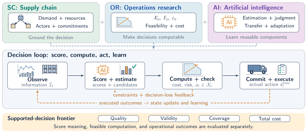
Figure 2.
Three distinct feedback targets. Formulation feedback revises an executable decision model; algorithm feedback improves a scoring program or search method; operational feedback updates beliefs and future decisions. The upper loops can supply reusable components to the operational loop [10,16,51]. Orange dashed arrows denote feedback; blue dashed arrows denote component reuse.
Figure 2.
Three distinct feedback targets. Formulation feedback revises an executable decision model; algorithm feedback improves a scoring program or search method; operational feedback updates beliefs and future decisions. The upper loops can supply reusable components to the operational loop [10,16,51]. Orange dashed arrows denote feedback; blue dashed arrows denote component reuse.
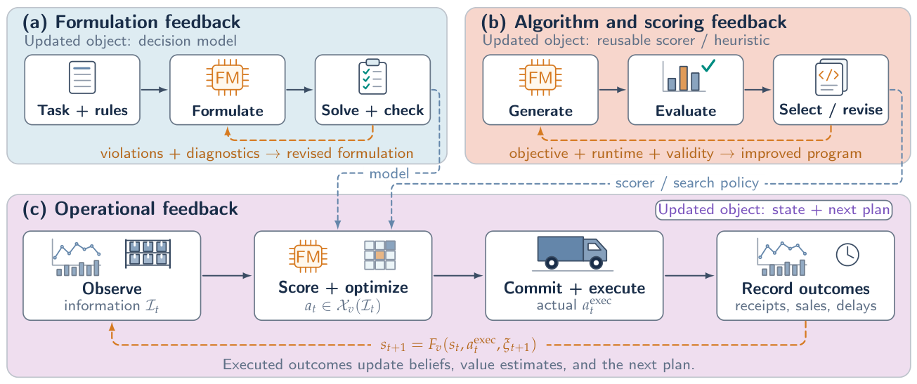
Figure 5.
Forward timing of the constructed shipment. Proposal and approval are , whereas actual dispatch is . For display, both shipments share a positive lead time L and intervening decisions are omitted. Executed quantities determine warehouse deductions and later receipts; the observation model determines how sales inform demand. A stock-exhausting sale includes the case and does not prove lost demand. Outcome records become available to subsequent decisions, closing the learning loop.
Figure 5.
Forward timing of the constructed shipment. Proposal and approval are , whereas actual dispatch is . For display, both shipments share a positive lead time L and intervening decisions are omitted. Executed quantities determine warehouse deductions and later receipts; the observation model determines how sales inform demand. A stock-exhausting sale includes the case and does not prove lost demand. Outcome records become available to subsequent decisions, closing the learning loop.
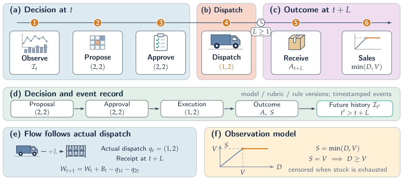
Table 2.
Four score semantics that a decision interface must distinguish. The first three can be learned inputs; the last includes a model of consequences.
Table 2.
Four score semantics that a decision interface must distinguish. The first three can be learned inputs; the last includes a model of consequences.
| Object | Meaning | Additional requirement for a decision |
|---|---|---|
| Outcome probability | Estimated frequency of a defined event under stated information and action | Costs of each outcome; population calibration; action-dependent response |
| Choice distribution | Relative support for the supplied alternatives under a specified question | Candidate coverage, admissibility, and a connection to operational value |
| Rubric score | Average or rating on declared criterion levels | Meaning of level spacing, tradeoff weights, and validation against the intended target |
| Decision value | Expected cost or utility of an action and its continuation | Correct horizon, feasible continuation, information, and uncertainty model |
Table 4.
Checks connecting a model output to an operational decision. Model confidence is an input to assessment, not a substitute for these checks.
Table 4.
Checks connecting a model output to an operational decision. Model confidence is an input to assessment, not a substitute for these checks.
| Interface | Question | Required connection |
|---|---|---|
| Semantic | Is the current task represented? | Entities, units, objective, constraints, and rule version |
| Informational | Are estimates and actions based on available information? | Cutoffs, observation model, and statistical support |
| Valuation | Does the score measure what the decision needs? | Event or rubric definition, cost units, horizon, calibration, and continuation value |
| Computational | Is the result admissible and of adequate quality? | Domains, residuals, feasible incumbents, bounds, or simulation estimates |
| Operational | Can the approved action be carried out as recorded? | Permissions, reservations, execution events, and outcome links |
Table 6.
Evidence for distinct system claims. Each row checks a different object; passing one row does not imply the next.
Table 6.
Evidence for distinct system claims. Each row checks a different object; passing one row does not imply the next.
| Evidence | Checked outcome | Reference object |
|---|---|---|
| Structured output / program | Type, parsing, execution, and output format | Declared schema, program, and runtime environment |
| Semantic formulation | Correct entities, units, objectives, and rules | Independently accepted decision specification |
| Mathematical solution | Feasibility, bounds, gap, and numerical residuals | Specified optimization model and domains |
| Statistical estimate | Calibration, decision risk, or intervention effect | Population, information set, and study design |
| Operational record | Dispatch, receipt, service, latency, and exceptions | Approved and executed actions with linked outcomes |
Disclaimer/Publisher’s Note: The statements, opinions and data contained in all publications are solely those of the individual author(s) and contributor(s) and not of MDPI and/or the editor(s). MDPI and/or the editor(s) disclaim responsibility for any injury to people or property resulting from any ideas, methods, instructions or products referred to in the content. |
© 2026 by the authors. Licensee MDPI, Basel, Switzerland. This article is an open access article distributed under the terms and conditions of the Creative Commons Attribution (CC BY) license (http://creativecommons.org/licenses/by/4.0/).
Copyright: This open access article is published under a Creative Commons CC BY 4.0 license, which permit the free download, distribution, and reuse, provided that the author and preprint are cited in any reuse.