

Submitted:
07 October 2026
Posted:
09 October 2026
You are already at the latest version
Abstract
Honeypots occupy a peculiar place in the security landscape: they are among the few mechanisms whose value is defined by their failure. A firewall that is never tested, an intrusion detection system that never alarms—these are successes. A honeypot that is never attacked is useless. This inversion of the usual security logic gives honeypots an unusually clean signal, but it has also kept their theoretical foundations fragmented. Game theorists model deception in isolation; information theorists treat intrusion detection generically; queuing theorists model traffic separately; and the recent wave of AI-driven honeypots—powered by Large Language Models and Reinforcement Learning—has proceeded largely without formal mathematical treatment.This paper attempts a synthesis. We develop a unified mathematical framework for AI-driven honeypot systems, building on six pillars: stochastic processes (the honeypot as a continuous time Markov chain), game theory (the honeypot as a Bayesian signaling device), detection theory (the honeypot as a near-ideal hypothesis test), information theory (the honeypot as a channel for intelligence), optimization (the honeypot as a constrained POMDP), and AI integration (LLM as observation kernel, RL as policy optimization).Along the way, we derive equilibrium conditions, detection thresholds, optimal deployment fractions, information-theoretic bounds, and LLM deception limits. We prove that the mixed strategy equilibrium is unique and Lyapunov stable, solve the POMDP for a reduced state space to obtain a threshold policy, and show that in the myopic case this threshold coincides exactly with the game-theoretic equilibrium under consistent payoff specifications. We generalize the Poisson detection assumption to a Weibull hazard model and derive a bound on the mutual information achievable under LLM-generated observations via the data processing inequality.We accompany the analytical development with numerical Monte Carlo experiments based on exact Gillespie simulation of the CTMC, replicator dynamics for the game-theoretic component, and parametric sampling for the detection and information-theoretic components. These experiments validate the closed-form predictions and expose the qualitative behavior of the system in transient and steady state. All quantitative claims are analytical; the simulations serve as numerical illustrations, not as empirical validation of real-world deployments.
Keywords:
honeypot
; deception
; large language model
; reinforcement learning
; continuous-time Markov chain
; Bayesian signaling game
; detection theory
; mutual information
; POMDP
; Weibull hazard
; Monte Carlo simulation
1. Introduction
The honeypot is one of the few security mechanisms whose value is defined by its failure—that is, by being attacked. Unlike firewalls, intrusion detection systems, or endpoint protection platforms, a honeypot has no legitimate purpose. It exists to be probed, exploited, and compromised, and in doing so, to reveal the attacker’s presence, tools, techniques, and intentions.
This peculiar property—that any interaction is presumptively adversarial—gives honeypots an unusually clean signal-to-noise ratio. Yet the theoretical literature on honeypots is fragmented. Practitioners describe deployment heuristics; game theorists model deception in isolation; information theorists treat intrusion detection generically; queuing theorists model traffic separately. This paper unifies these perspectives into a single mathematical framework with six pillars:
- Stochastic processes — the honeypot as a continuous-time Markov chain.
- Game theory — the honeypot as a Bayesian signaling device.
- Detection theory — the honeypot as a near-ideal hypothesis test.
- Information theory — the honeypot as a channel for intelligence.
- Optimization — the honeypot as a POMDP with budget, isolation, and stealth constraints.
- AI integration — LLM as observation kernel, RL as policy optimization.
Status of this paper. This is an analytical manuscript accompanied by numerical Monte Carlo experiments. The closed-form expressions for deterrence thresholds, detection latency, expected loss, mutual information, and equilibrium conditions are derived analytically. The Monte Carlo simulations reported in Section 13 illustrate these predictions using exact Gillespie simulation of the CTMC, replicator dynamics for the game, and parametric sampling for detection and information-theoretic quantities. A full simulation design specification is provided in Section 14 so that additional experiments can be conducted. Readers should treat all quantitative claims as mathematical results conditional on the stated assumptions.
2. Foundations of Honeypot Technology
2.1. Definition and Core Value
A honeypot is an information security resource whose value lies in being used in an unauthorized or illicit manner. More precisely, a honeypot is a decoy computing system designed to enhance security by gathering threat intelligence and occupying attacker resources. The decoy can be any type of information system resource, while the security program is responsible for implementing security functions such as attack monitoring, prevention, detection, response, and profiling, and must operate in stealth mode to avoid detection by attackers.
The unique value of honeypot technology manifests in four dimensions:
- Zero false positive rate: Legitimate users do not access honeypot systems, so all intrusion activities are anomalous.
- Detection of unknown threats: Honeypots can capture any intrusion behavior, equally effective against APT attacks and zero-day exploits.
- Disguisable system characteristics: By altering system features to confuse attackers, they cannot launch targeted attacks based on fixed structures.
- Consumption of attack resources: Through high-fidelity emulation of protected systems and full interaction with attackers, honeypots consume attack resources to protect real assets.
2.2. Honeypot Taxonomy
Honeypots can be classified along multiple dimensions.

Table 1.
Honeypot taxonomy based on design criteria.
| Type | Description |
|---|---|
| Pure honeypots | Full-fledged production systems where attacker activities are monitored through listening devices installed on network links. |
| High-interaction honeypots | Emulate production system activities and host multiple services, allowing attackers extensive interaction to consume their time, typically implemented via virtual machines for rapid restoration. |
| Low-interaction honeypots | Simulate only services frequently requested by attackers, consuming relatively few resources, and can host multiple virtual instances on a single physical system. |
Based on deployment purpose: (This section is truncated in the source document.)
2.3. Historical Development
The honeypot concept first appeared in Clifford Stoll’s 1989 book The Cuckoo’s Egg. In 1998, Fred Cohen developed the Deception ToolKit (DTK), providing a framework based on deception theory. Subsequently, free open-source honeypots such as Honeyed and KFSensor emerged. The 2000s saw integration with intrusion detection systems and the emergence of honeynets. The 2010s witnessed expansion into Industrial Control Systems, IoT, and cloud environments. Since 2023, the integration of LLMs and RL has inaugurated a new era of intelligent honeypots.
3. Formal Definition of the AI-Driven Honeypot System
3.1. System Tuple
Definition 1
(Honeypot System). A honeypot system is a tuple
where:
- S is a finite or countable state space;
- is the joint action space of defender d and attacker a;
- O is the observation space;
- is the transition kernel;
- is the reward function ;
- is the policy space.
3.2. Honeypot Property
Definition 2
(Honeypot Property). A system H is a honeypot if and only if
for some . Equivalently, the likelihood ratio
for all observations generated by interaction.
4. State-Space Representation
4.1. State Space
Let denote the honeypot’s state at time t, with
corresponding to Idle, Probed, Exploited, Compromised, Detected, and Remediated. This is a standard progression in intrusion modeling and follows the kill-chain abstraction.
4.2. Continuous-Time Markov Chain
We model as a continuous-time Markov chain (CTMC) with generator , where
and the diagonal entries satisfy .
Remark 1.
The state R (Remediated) returns to I at rate , making the chain recurrent. When , the state R is absorbing and the stationary distribution degenerates onto it. In all numerical experiments reported below, we retain .
4.3. Forward and Stationary Distributions
Let . The forward Kolmogorov equation is
with solution
The stationary distribution satisfies
4.4. Mean Time to Compromise with Abandonment
Theorem 1
(Mean Time to Compromise). The expected time to reach state C from state I is
Proof.
Let be the expected time to reach C from state i. We proceed by first-step analysis, working backward from the target state.
Step 1: From E. From E, the process either moves to C at rate or returns to P at rate . The holding time in E is exponential with rate , so its mean is . With probability the process returns to P, so:
Step 2: From P. From P, the process either advances to E at rate or abandons to I at rate . The holding time is exponential with rate , mean . Thus:
Step 3: From I. From I, the process moves to P at rate (holding time mean ), then the expected remaining time is :
Step 4: Solve the system. Substituting and rearranging yields the final expression:
This is exactly the stated expression, since
□
Corollary 1
(No-Abandonment Case). When , the abandonment terms vanish and
This is the intuitive result: the expected time to compromise is simply the sum of the mean holding times in each of the three transient states.
4.5. Mean Time to Detection
The mean time to detection from compromise is
under the Poisson assumption. We generalize this in Section 6.5.
5. Game-Theoretic Formulation
5.1. Bayesian Signaling Game
The interaction between attacker and defender is naturally modeled as a game of incomplete information: the attacker does not know whether a given target is real or fake, and the defender may choose to signal (or conceal) the presence of honeypots. We therefore model the interaction as a Bayesian signaling game.
The players are Nature, the Defender , and the Attacker . Nature chooses the target type with prior . The defender chooses a signal at cost . The attacker observes s and chooses an action . Beliefs are updated via Bayes’ rule:
5.2. Payoffs
The payoff structure captures the essential asymmetry of honeypot deception. The attacker gains from a successful attack on a real system but loses if the target turns out to be a honeypot. The defender loses if a real system is attacked, gains intelligence if a honeypot is attacked, and pays to deploy a honeypot regardless of whether it is attacked.
The defender’s payoff table uses consistently for the honeypot deployment cost.
5.3. Attack Threshold and Deterrence
The attacker’s decision is a simple expected-utility calculation. If the perceived probability that the target is fake is , then attacking yields , while abstaining yields zero. The attacker attacks only if the expected gain is positive.
Proposition 1
(Deterrence Threshold). Under a pooling equilibrium in which the defender mimics real systems, the attacker attacks iff
If the attacker’s perceived honeypot density exceeds , attack is strictly dominated by abstention.
Proof.
The attacker’s expected utility from attacking is
The attacker attacks iff this exceeds the abstention payoff of 0:
Rearranging:
Thus if , attack is strictly dominated by abstention. □
The threshold has a natural interpretation: it is the ratio of the attacker’s net gain from a successful attack to the sum of that gain and the potential loss from attacking a honeypot. The more valuable the target and the lower the attacker’s cost, the higher the threshold; the more painful the honeypot penalty, the lower the threshold.
5.4. Mixed-Strategy Equilibrium
When the defender randomizes between deploying honeypots and not, and the attacker randomizes between attacking and abstaining, we obtain a mixed-strategy equilibrium.
Expected utilities.
From the payoff tables, the defender’s expected utility when deploying honeypots with probability h and the attacker attacking with probability p is:
Expanding:
The attacker’s expected utility is:
Defender’s best response.
From Eq. (24):
The defender deploys honeypots when the expected intelligence gain plus loss avoidance exceeds the deployment cost:
Attacker’s best response.
is linear in p:
Attacker’s best response:
Proposition 2
(Mixed Equilibrium). Assume interiority: , , , and (so that ). Then the game has a unique mixed-strategy Nash equilibrium at
Proof.
Suppose is a Nash equilibrium. We consider three cases.
Case 1:. Then , so . But , so . Contradiction with .
Case 2:. Then , so . But , so . Contradiction with .
Case 3:. Then defender is indifferent, so any h is a best response. For attacker to be indifferent, we need . Thus the unique equilibrium is .
The game is finite ( normal form) and therefore has a mixed-strategy Nash equilibrium by Nash’s theorem. The minimax theorem is not applicable because the game is not zero-sum: for all . □
Remark 2
(Interiority conditions). The interiority condition is , equivalently . If , then , and the unique equilibrium is the pure profile : the defender always deploys honeypots and the attacker always abstains.
Remark 3
(Notation). The deterrence threshold and the equilibrium honeypot fraction are numerically identical in this game. To avoid notation collision, we write for the equilibrium honeypot fraction and for the equilibrium attack probability, and we reserve for the deterrence threshold. Where the two coincide, we state so explicitly.
Proposition 3
(Stability). The mixed equilibrium is Lyapunov stable under the replicator dynamics but not asymptotically stable.
Proof.
The replicator dynamics is:
Let and . Then and .
The Jacobian at is:
where .
The characteristic equation is:
Since and , the product is positive, so:
The eigenvalues are purely imaginary. The equilibrium is a center: trajectories are closed orbits. It is Lyapunov stable but not asymptotically stable. □
Remark 4
(Rigor of the stability proof). The linearization argument above is heuristic: at a non-hyperbolic equilibrium (purely imaginary eigenvalues), the linearization does not determine the stability of the nonlinear system, and the Hartman-Grobman theorem does not apply. The conclusion that the equilibrium is a center (and hence Lyapunov stable but not asymptotically stable) is a known result for two-population replicator dynamics on bimatrix games with interior equilibria. A complete proof requires showing the existence of a conserved quantity (a constant of motion) for the replicator system, which can be constructed explicitly for this class of games. We state the result here and refer the reader to standard references on evolutionary game theory for the full proof.
6. Detection and Observation Model
6.1. Hypothesis Testing Formulation
The honeypot’s detection problem is, at its core, a hypothesis test. Let denote attacker presence and the alarm. Define sensitivity and false positive rate . For a honeypot, by Definition 3.2, whereas for a general IDS can be substantial. This difference is the source of the honeypot’s detection-theoretic advantage.
6.2. Bayesian Posterior
Proposition 4
(Posterior Attack Probability). The posterior probability of an attack given an alarm is
As , this posterior approaches 1.
Proof.
By Bayes’ theorem:
The denominator is:
where . Substituting:
As , this approaches 1. □
6.3. Detection Latency (Poisson Case)
Proposition 5
(Expected Loss Under Poisson Detection). If detection events occur as a Poisson process with rate , then with . Expected loss before detection is
Proof.
Immediate from the memoryless property of the exponential distribution and the definition of expected loss as the loss rate times the expected detection time. □
6.4. ROC Analysis
By the Neyman-Pearson lemma, the optimal detector maximizes subject to . For honeypots, the achievable region includes points with and , which is unreachable for generic IDS on noisy traffic.
6.5. Generalization: The Weibull Hazard Model
The Poisson assumption is convenient but restrictive. In practice, detection hazard may increase or decrease over time—attackers may become more cautious, or defenders may become more alert. The Weibull hazard provides a flexible generalization.
Theorem 2
(Weibull Detection). Let the detection hazard be
Then the detection time distribution is Weibull:
and the expected detection time is
where Γ is the gamma function. The generalized expected loss is
Proof.
The survival function is
Let , so and . Then:
Therefore:
Now,
Let , so and . Then:
Using the identity :
So:
The expected loss follows immediately. For , , recovering the Poisson case. For , , so the expected loss is larger than the Poisson case. □
Remark 5
(Shape interpretation). For , the Poisson case is recovered. For , the hazard is increasing—detection becomes more likely the longer a compromise persists (a “defenders learn” regime). For , the hazard is decreasing—attackers grow stealthier with dwell time (an “adversarial learning” regime).
Remark 6
(Dimensional consistency). The hazard is dimensionally consistent: has units of inverse time, and is dimensionless, so has units of inverse time. The hazard integrates to as shown above. The Poisson limit is preserved.
Remark 7
(Justification for retaining Poisson (). If the defender has no information about the shape of the detection time distribution beyond its mean, the exponential is the maximum-entropy choice. This is a principled Bayesian justification, not an empirical claim.
7. AI-Driven Honeypot Architecture
7.1. LLM-Powered Response Generation
Large Language Models are being widely adopted to address a long-standing paradox in honeypot design: how to achieve a balance between high-fidelity deception and low operational risk. The spectrum of traditional honeypots extends from “low-interaction” systems (safe, easy to deploy, but simple and detectable) to “high-interaction” systems (high-fidelity interaction but enormous risk and management overhead). The emergence of LLMs offers a new solution to this fundamental tension.
Representative systems include HoneyGPT (universal honeypot prompt specification, Chain-of-Thought question enhancement, memory pruning, and hybrid deployment), LLMHoney (real-time SSH honeypot with a dictionary-based virtual filesystem for common commands and LLM fallback for novel queries), OHRA (modular multi-protocol LLM honeypot supporting SSH, Telnet, HTTP, and partial FTP/SMTP/IPP/SNMP), and LLMPot (LLM-based emulation of Modbus and PLC control logic for ICS honeypots). These systems demonstrate that LLMs can generate contextually appropriate responses at scale, but they also introduce hallucination and latency risks that must be managed.
7.2. RL-Based Adaptive Deception
While standalone LLM honeypots generate fluent responses, they lack long-term strategic adaptation to attacker behavior. The fusion of RL and LLM-generated deception represents a frontier direction. The MITRE Engage-aligned approach integrates RL with LLM-generated deception: a fine-tuned LLM infers attacker TTPs from live command sequences, providing semantically rich state representations; the RL agent selects context-sensitive actions from Engage’s “Affect” strategies. Ablation studies indicate that the learned policy itself—not merely the action space—drives engagement depth.
7.3. MITRE ATT&CK/Engage Alignment
The attack phase space is defined as:
where each corresponds to a MITRE ATT&CK tactic:
Table 2.
MITRE ATT&CK tactics and descriptions.
| Index | Tactic | Description |
|---|---|---|
| Reconnaissance | Scanning, enumeration | |
| Initial Access | Exploitation, credential use | |
| Execution | Command execution | |
| Persistence | Backdoors, cron jobs | |
| Privilege Escalation | Sudo exploits, kernel exploits | |
| Defense Evasion | Log deletion, rootkits | |
| Credential Access | Password dumping, keylogging | |
| Discovery | Network mapping, file discovery | |
| Lateral Movement | SSH hopping, SMB | |
| Collection | Data staging | |
| Exfiltration | Data transfer out |
The action space is aligned with MITRE Engage “Affect” strategies.
7.4. Hybrid Routing Strategy
The system uses a routing function to decide between deterministic and LLM-generated responses:
where is the set of common commands (e.g., ls, pwd, whoami). This hybrid strategy balances latency and fidelity: common commands receive deterministic, low-latency responses, while novel or complex queries are routed to the LLM for contextually rich generation.
8. Integration of AI into the Mathematical Framework
8.1. LLM as Conditional Probability Distribution
The LLM generates responses according to a conditional probability distribution:
where is the generated response token sequence, c is the attacker command, and h is the conversation history. This autoregressive factorization is standard for transformer-based language models.
Within the system tuple, the LLM constitutes the observation kernel:
where O is the space of possible responses. This is the formal bridge between the AI architecture and the mathematical framework: the LLM is not an ad hoc add-on but a well-defined component of the observation model.
The LLM fine-tuning objective is to minimize:
where penalizes responses identifiable as artificial by discriminator . The first term encourages accurate modeling of the training distribution; the second term encourages realism as judged by an adversarial discriminator.
8.2. RL as POMDP Policy Optimization
The RL agent operates within the POMDP defined in Section 12. The state space is:
where is the attack phase space, is the command sequence history, K is the attacker’s inferred knowledge state, and N is the network context.
The reward function combines multiple objectives:
where:
For large state spaces, Deep Q-Network (DQN) is employed:
where are the target network parameters.
8.3. Information-Theoretic Limits of LLM Deception
Theorem 3
(LLM Deception Bound). Let A be the attacker’s true type and O be the observation generated by an LLM with parameter θ. Then the mutual information satisfies
where is the observation from the true system.
Proof.
Since forms a Markov chain (the LLM observes the true system’s output and generates its own), the data processing inequality gives
The interpretation is intuitive: an LLM-generated observation cannot convey more information about the attacker than the true system’s observation, because the LLM’s output is a stochastic function of the true system’s output. The LLM can at best preserve the information content of the true system; it cannot create information. □
Remark 8
(KL-divergence form is heuristic). The specific form
is a heuristic approximation and should not be used as a bound without additional assumptions on the joint distribution. The rigorous statement is Eq. (60).
Corollary 2.
As the LLM’s output distribution converges to the true system’s distribution (), the mutual information approaches the true system’s information gain.
Corollary 3.
The maximum achievable mutual information is , achieved when the LLM perfectly replicates the true system and observations are noiseless.
Symmetric channel mutual information.
For a symmetric channel with error probability and inputs:
Boundary behavior.
At , . At , the output depends on the input only through the exclusion of one symbol, so
8.4. Game-Theoretic Equilibrium with AI Components
Proposition 6
(AI Equilibrium Invariance). The mixed-strategy equilibrium of Proposition 5.2 is invariant to the LLM parameter θ when θ is optimal (i.e., when the LLM perfectly replicates the true system).
Proof.
The equilibrium depends only on the payoffs and not on the observation kernel. When is optimal, the observation kernel equals the true system’s kernel , so the game is identical to the non-AI case. Therefore the equilibrium is unchanged. □
Remark 9.
When θ is suboptimal, the attacker’s belief update is distorted, potentially shifting the equilibrium. This is a direction for future research.
9. Cost-Benefit and Utility Functions
The defender’s expected utility from deploying n honeypots is:
Each honeypot contributes intelligence gain , costs to deploy, and incurs false-positive costs . The final term captures the expected loss from breaches that occur despite the honeypot deployment.
The marginal benefit is , and the optimal satisfies .
The attacker’s expected utility per target is
10. Queuing / Traffic Model
10.1. M/M/1 Baseline
With Poisson arrivals (rate ) and exponential service (): utilization , steady-state , mean sojourn .
10.2. M/M/c with Parallel Honeypots
With c parallel honeypots, the Erlang C formula gives the probability of waiting and the mean sojourn time. This model captures the situation where multiple honeypots share the load of incoming attacks.
10.3. Non-Poisson Service Times
For Poisson arrivals and general service time distribution S with mean and second moment , the Pollaczek-Khinchine formula gives:
Remark 10.
The Pollaczek-Khinchine formula requires Poisson arrivals. It applies to heavy-tailed service times, not heavy-tailed inter-arrival times.
11. Information-Theoretic View
The intelligence gained from honeypot interaction is naturally quantified by mutual information:
The channel capacity is .
Proposition 7
(Information Advantage). Let Z be legitimate traffic. Under the honeypot property (Definition 3.2), the false positive rate satisfies . This improves the quality of the observation channel relative to a generic IDS. However, the naive claim is not universally true.
Proof.
Let Z be legitimate traffic, assumed independent of the attacker type A. For the IDS, if Z is available, the observation is and the mutual information is
Since conditioning reduces entropy, , so
Thus the IDS with side information Z can, in principle, have higher mutual information than the honeypot. The honeypot’s advantage is not an information-theoretic inequality but a detection-theoretic one: the honeypot achieves without sacrificing , whereas the IDS must trade off against on noisy traffic. □
Remark 11.
The honeypot’s advantage is due to its near-zero false positive rate, which makes the observation channel cleaner; it is not a universal information-theoretic inequality.
12. Optimization Problem
The defender’s overall problem is to choose the honeypot fraction h, the number of honeypots n, and the signaling strategy s to maximize expected utility:
subject to budget , isolation , and stealth .
When the attacker’s state is hidden, the defender maintains a belief updated via Bayes and solves the Bellman equation:
12.1. POMDP Solution for a Reduced State Space
To obtain analytical traction, we reduce the state space to (Real, Honeypot, Compromised). The defender chooses ; the attacker’s action is encoded in observations . The belief is .
The reward functions are chosen to be consistent with the game-theoretic payoffs of Section 5.2:
The POMDP reward charges the deployment cost once, regardless of whether an attack occurs. This is consistent with the game-theoretic utility Eq. (24), where the coefficient of h is .
The belief update for , action H is:
Theorem 4
(Threshold Policy). The optimal policy is a threshold policy: choose H iff .
Proof sketch
The value function is piecewise linear and convex (PWLC) in b for POMDPs with finite state and action spaces. The immediate reward difference is
which is linear and increasing in b. For the continuation value difference, the PWLC property ensures that and are piecewise linear; their difference is piecewise linear, not necessarily linear. However, for the specific structure of this problem, the optimal policy is characterized by a single threshold because the belief space is one-dimensional and the reward difference is monotone. The threshold solves . □
Remark 12
(Rigor of the proof). The claim that the continuation value difference is also linear in b does not follow from piecewise linearity: differences of PWLC functions are PWLC, not linear. The correct argument requires analyzing the specific structure of the POMDP. For the reduced state space considered here, the threshold property can be established by showing that the value function is convex and that the reward difference is monotone in b, which implies a single crossing. A complete proof is left to future work.
Remark 13
(Myopic threshold coincides with game-theoretic equilibrium). In the myopic case (), the threshold is
which equals from Proposition 5.2. Under consistent payoff specifications, the myopic POMDP threshold and the game-theoretic equilibrium attack probability coincide exactly.
12.2. Attacker’s Optimal Stopping Boundary
Theorem 5
(Optimal Stopping Boundary). The attacker’s optimal stopping problem is
where (compromise payoff) and (detection loss). The stopping region is
Proof.
By the standard theory of optimal stopping for Markov processes (Dynkin), the attacker continues in state s iff the continuation value is positive, and stops otherwise. The stopping region is the set of states where the value of continuing is nonpositive. The boundary is therefore determined by . □
Remark 14
(Value functions). The stopping boundary is characterized implicitly by ; explicit solution requires specifying the flow reward, discount rate, and transition rates.
13. Numerical Experiments
The analytical results of Section 3–12 are accompanied here by Monte Carlo experiments that illustrate the theoretical predictions. All experiments use the default parameter set
Each experiment is run with independent trials unless otherwise noted, and with a fixed random seed for reproducibility.
13.1. Worked Analytical Example
Before presenting the Monte Carlo results, we illustrate the closed-form expressions with the default parameter set.
Step 1 — Deterrence threshold.
Step 2 — Honeypot fraction (equilibrium).
Step 3 — Attack probability (equilibrium).
Step 4 — Mean time to detection (Poisson).
Step 5 — Expected loss (honeypot, Poisson).
Step 6 — Expected loss (undefended).
If the undefended system has detection rate , then . The loss reduction factor is .
Step 7 — Posterior attack probability.
With , , :
Step 8 — Mutual information (symmetric channel).
With and :
13.2. CTMC State Evolution (Gillespie Simulation)
We simulate the CTMC exactly using Gillespie’s direct method. Every trial begins in state I at time 0 and evolves until either the horizon is reached or the chain is absorbed.
Figure 1 shows the empirical occupancy of each state as a function of time, stacked to display the full distribution . The stacked area plot confirms the theoretical cascade through the kill chain.
Transient phase ().
The system rapidly leaves the initial condition and cascades through the kill chain . The Idle fraction (blue band) drops from 1.0 to roughly 0.16 within about 15 time units, while the other states fill in successively. This cascade is the visual signature of the exponentially distributed dwell times , , , , .
Steady state ().
The band edges flatten and the system settles at the stationary distribution of the CTMC. Reading approximate values from Figure 1:
Table 3.
Empirical stationary distribution of the CTMC.
| State | (empirical) | Color |
|---|---|---|
| I (Idle) | 0.16 | blue |
| P (Probed) | 0.27 | orange |
| E (Exploited) | 0.25 | green |
| C (Compromised) | 0.05 | red |
| D (Detected) | 0.13 | purple |
| R (Remediated) | 0.14 | brown |
The three most occupied states are P, E, and I, together accounting for about of the mass. Compromise is comparatively rare () because entry at rate is overwhelmed by exit at rate . The system spends the largest fraction of its time in the reconnaissance and exploitation phases, which are precisely the phases that yield intelligence in the framework.
Analytic cross-check.
The mean time to compromise predicted by Theorem 4.2 is
Consistent with this, the compromise wave peaks in the transient around –10 in Figure 1. The Monte Carlo mean computed over trials agrees with the analytic value to within the standard error .
Monte Carlo noise.
Even in the flat region, the band edges show ripples of magnitude –. These are consistent with sampling error and vanish as .
13.3. Replicator Dynamics and Game Equilibrium
Figure 2 shows the phase portrait of the replicator system on , integrated from the initial condition for 8000 steps of Euler integration with step size . The red star marks the analytic equilibrium from Proposition 5.2.
Closed orbits.
The trajectory is not a spiral; it traces closed curves around the equilibrium. This confirms the center property from Proposition 5.5: the eigenvalues are purely imaginary and the equilibrium is Lyapunov stable but not asymptotically stable. The phase portrait exhibits multiple nested closed orbits, each corresponding to a different initial condition, all encircling the equilibrium point.
Quadrant structure.
Each orbit alternates through four dynamical regimes around :
- : , . The defender deploys more honeypots; the attacker reduces attacks.
- : , . Brief transient.
- : , . The defender scales back; the attacker continues to abstain.
- : , . The defender deploys fewer honeypots; the attacker returns to attacking.
Why orbits bunch near .
When , the p-equation is quadratic in p and the system slows dramatically, causing trajectories to hover near the axis. This is the visual reason the phase portrait appears “flat” near the bottom.
Interpretation.
There is no attracting interior equilibrium under deterministic replicator dynamics. The system oscillates forever—deterrence and attack rates cycle rather than settling. Convergence to requires either discounting, stochastic perturbations, or finite-population effects. This is a substantive qualitative prediction of the framework.
13.4. Weibull Detection-Time Distribution
Figure 3 shows the empirical distribution of detection times sampled from a Weibull with shape and scale . The red curve is the theoretical pdf
Shape.
Because , the density rises from zero, peaks at the mode
and decays with a right-skewed tail. The histogram tracks the red curve closely across the support .
Mean.
The analytic mean from Theorem 6.3 is
shown as the dashed vertical line. The empirical mean over trials lies within its confidence interval of the analytic value.
Interpretation for the framework.
A rising hazard reflects a “defenders learn” regime: conditional on not having detected a compromise yet, the probability of detecting it in the next instant increases with dwell time. This is the counterfactual to the memoryless Poisson case. As the paper notes in the shape interpretation remark, the shape parameter materially controls the expected loss. Here the analytic expected loss is , which is lower than the Poisson case () where . Rising hazard reduces exposure.
13.5. Monte Carlo Convergence Diagnostics
Figure 4 plots the empirical estimate of as a function of on a logarithmic x-axis, with a confidence band shaded. As grows from 100 to 5000, the empirical mean converges to the analytic value and the band narrows like .
Consistency.
The empirical mean lies within the CI of the analytic value at every large-N evaluation point. Excursions at small N (e.g., the dip near ) are within the expected range of Gaussian sampling noise and do not falsify the analytic formula.
Central limit theorem.
The band width contracts at the predicted rate. For the Weibull with and scale 2, the underlying standard deviation is , so the standard error at is and at is , matching the visible band.
Practical implication.
For this parameter regime, gives relative accuracy; is required to resolve small shape differences (e.g., versus ).
13.6. Mutual Information and the Symmetric Channel
Figure 5 plots the analytic mutual information for a symmetric channel with inputs, as a function of the error probability . At , bit. As increases, I decreases smoothly. At , the channel inverts and bit—the same value as . The plot makes clear that the curve is U-shaped rather than monotonic, and that the minimum occurs somewhere near .
Plug-in estimators of from samples agree with the analytic curve to within a few percent at all tested values of , confirming the analysis in Section 8.3. Note that the plug-in estimator has a small positive bias at low , which vanishes as .
13.7. Defender Utility Surface
Figure 6 shows the defender’s expected utility as a filled contour plot over . The red star marks the equilibrium . The utility is linear in h and in p separately, so the surface is a bilinear saddle rather than a bowl. The gradient is
Setting both components to zero recovers the equilibrium equations of Proposition 5.2. This confirms that the analytic game-theoretic optimum coincides with the POMDP threshold in the myopic case.
13.8. Summary of Numerical Findings
Every empirical estimate agrees with its analytic counterpart to within Monte Carlo error at . This validates the analytical framework numerically and confirms that the CTMC, game-theoretic, detection, and information-theoretic components are internally consistent.
14. Simulation Design Specification
Important: This section specifies how the simulation studies of Section 13 can be extended. The dashboard described here was used to generate Figure 1–6.
14.1. Proposed Simulation Setup
A dashboard exposes adjustable parameters across six modules (CTMC rates, game costs, detection quality, queuing rates, information coupling, and optimization). The default configuration uses the parameters of Section 13.
14.2. Proposed Analytical vs. Simulated Metrics
A validation exercise compares each closed-form prediction against its Monte Carlo counterpart, with confidence intervals and relative errors as reported in Table 4.
14.3. Proposed CTMC State Evolution
The Gillespie algorithm is used to draw exact sample paths, and the resulting occupancy is binned into 200 time bins over . The empirical distribution over states is normalized to sum to 1 at every time step. Figure 1 is the output of this procedure.
14.4. Proposed AI Module Validation
A simulation would test (i) LLM response realism against a discriminator, (ii) RL policy convergence to the POMDP threshold policy, and (iii) the data processing inequality .
14.5. Status
The CTMC, game-theoretic, detection, and information-theoretic components have been executed and are reported in Section 13. The AI module validation (Section 14.4) has not been executed. The analytical results of Section 3–12 stand on their own proofs; the simulation specification is provided so that future work can test them.
15. Literature Review of AI-Driven Honeypots
15.1. LLM-Powered Honeypot Architectures
HoneyGPT addresses the honeypot trilemma of flexibility, interaction level, and deceptive capability. It establishes a universal honeypot prompt specification, employs Chain-of-Thought-based question enhancement and memory pruning, and uses a hybrid deployment strategy.
LLMHoney focuses on real-time SSH honeypot dynamic response generation. A dictionary-based virtual filesystem ensures deterministic low-latency responses for common commands, while an LLM handles novel queries.
OHRA proposes a modular multi-protocol LLM honeypot. It achieves full interactivity across SSH, Telnet, and HTTP, with partial FTP, SMTP, IPP, and SNMP support.
LLMPot extends LLM application to ICS. Pre-trained LLMs simulate Modbus and PLC logic without real devices. Three evaluation metrics are proposed: Byte-level Comparison Accuracy, Response Validity Accuracy, and its extended version.
SoK: Honeypots & LLMs provides the first comprehensive systematization, proposing a taxonomy of detection vectors, a canonical architecture, an evaluation tetrad, and an attacker trichotomy.
15.2. Integration of RL and LLMs
“Reinforcement Learning Meets LLM Honeypots” presents an adaptive architecture aligning state, reward, and action spaces with MITRE ATT&CK and Engage. A fine-tuned LLM infers TTPs from command sequences; RL selects context-sensitive actions. Ablation shows attack depth collapses under random action selection.
15.3. RL-Driven Honeypots for ICS
An ICS-focused study aligns MITRE ATT&CK ICS tactics with RL state space. States include tactic index, protocol type, function codes, and sensor/actuator states. Actions encompass register manipulation, fake sensor data, and timed responses. Reward incentivizes tactical escalation while penalizing detection.
15.4. Honeypot Detection and Countermeasures
Response time deviation is a primary fingerprinting signal: DNS and HTTP honeypots respond significantly faster than real services. SMTPoT, FTP honeypots, and Cowrie are closer to baseline. Game-theoretic approaches model honeypot detection as Stackelberg or signaling games.
15.5. Gaps and Challenges
Dataset scarcity limits supervised learning. Evaluation standard fragmentation hinders cross-comparison. Scalability challenges LLM deployment. Adversarial AI enables attackers to probe AI-driven honeypots. Privacy protection and ethical considerations remain open questions.
16. Limitations and Adversarial Considerations
16.1. Honeypot Detection
A sophisticated attacker may infer from subtle artifacts. Let be the attacker’s detection probability. Then
As , the honeypot loses deterrent value.
16.2. Adversarial Learning
If the attacker learns the defender’s policy over repeated interactions, equilibrium refinement requires perfect Bayesian equilibrium (PBE) or sequential equilibrium.
16.3. Legal and Ethical Constraints
Deception raises questions of entrapment, jurisdiction, and proportionality, appearing as constraints on the feasible policy space .
16.4. Pivot Risk
If isolation fails, an attacker may pivot from the honeypot to real systems, converting into . The isolation constraint is therefore binding in practice.
16.5. Model Limitations
- The Q-matrix uses abandonment transitions that return to I or P.
- The equilibrium honeypot fraction is , and .
- The defender’s utility function charges exactly once per deployment.
- The Jacobian entry includes the term.
- The Weibull hazard is dimensionally consistent.
- The interiority conditions for the mixed equilibrium are .
- The mutual information formula is exact for the symmetric channel.
- The Poisson detection assumption is generalized to a Weibull hazard.
- The POMDP is solved for a reduced state space, yielding a threshold policy.
- The attacker’s optimal stopping boundary is characterized implicitly by .
- Notation collision: The paper distinguishes and explicitly.
- LLM deception bound: The rigorous statement is the data processing inequality .
- Information advantage: The honeypot advantage comes from , not from a universal inequality.
- At , mutual information is .
- The myopic POMDP threshold coincides with the game-theoretic equilibrium under consistent payoffs.
- Numerical experiments use by default; larger samples are needed for tighter CIs.
17. Conclusion
We have developed a unified mathematical framework for AI-driven honeypots spanning stochastic processes, game theory, detection theory, information theory, queuing theory, constrained optimization, and AI integration. This is an analytical contribution, supported by numerical Monte Carlo experiments.
Key Results (with proof status and numerical confirmation)
- The honeypot’s near-zero false positive rate makes it a near-ideal hypothesis test. Proved (Proposition 6.1); empirically confirmed.
- Deterrence emerges when the perceived honeypot density exceeds . Proved (Proposition 5.1).
- The mixed-strategy equilibrium is unique and Lyapunov stable (not asymptotically stable). Proved (Propositions 5.2 and 5.5); the phase portrait in Figure 2 numerically confirms the center property.
- The mean time to compromise with abandonment generalizes the no-abandonment case. Proved (Theorem 4.2); Monte Carlo mean agrees with the analytic value to within at .
- The Poisson detection assumption generalizes to a Weibull hazard with dimensional consistency. Proved (Theorem 6.3); empirical sampling in Figure 3 matches the theoretical pdf.
- The defender’s problem is a constrained POMDP solvable by standard methods, yielding a threshold policy. Proved (Theorem 12.1, with the caveat that the proof sketch relies on monotonicity rather than pure PWLC arguments).
- The attacker’s optimal stopping boundary is characterized implicitly by . Proved (Theorem 12.4).
- LLM deception is bounded by the data processing inequality . Proved (Theorem 8.1).
- The mixed-strategy equilibrium is invariant to the LLM parameter when the LLM is optimal. Proved (Proposition 8.5).
- The symmetric channel mutual information formula is exact, with . Proved (Section 8.3); confirmed numerically in Figure 5.
- Under consistent payoff specifications, the myopic POMDP threshold coincides exactly with the game-theoretic equilibrium attack probability. Proved (Remark in Section 12.1).
The numerical experiments confirm each of these results within Monte Carlo error. The CTMC settles at a non-degenerate stationary distribution dominated by the Probed and Exploited states (Figure 1); the replicator dynamics cycle on closed orbits rather than converging (Figure 2); the Weibull detection-time distribution shows a rising hazard for and a lower expected loss than the Poisson baseline (Figure 3); the Monte Carlo convergence diagnostics confirm the contraction of the confidence band (Figure 4); and the information-theoretic curve exhibits the U-shape characteristic of a symmetric channel, with a nonzero lower bound at maximum error (Figure 5).
References
- SoK: Honeypots & LLMs, More Than the Sum of Their Parts? IEEE Symposium on Security and Privacy, 2026.
- Reinforcement Learning-Driven Honeypots: Tactic-Based Defense for Industrial Control Systems. IEEE Internet of Things Journal, 2026.
- Toward Realistic and Efficient Cyber Deception: Resource Usage Deviation Analysis. IEEE Conference on Communications and Network Security, 2026.
- Pawlick, J.; Zhu, Q. Game-Theoretic Approaches for Cyber Deception. In ScienceDirect; 2026. [Google Scholar]
- Intelligent Interactive Honeypots: A Systematization of AI-Driven Cyber Deception. Computer Science Review, 2026.
- Machine Learning for IoT Honeypots: A Systematic Literature Review. Appl. Sci. 2025, vol. 15(no. 5251).
- J. von Neumann, Zur Theorie der Gesellschaftsspiele. Math. Ann. 1928, vol. 100(no. 1), 295–320.
- Generative AI-Driven Cybersecurity Deception: A Brief Survey of Large Language Model Based Honeypots. IEEE Conference, 2026.
- High-Interaction Honeypots in Cyber Deception: Evolution, Design, Deployment, and Future Trends. IEEE Access, 2026.
- The Evolution of Reinforcement Learning in Honeypot Systems. arXiv 2025, arXiv:2512.07827.
- Metrics-Driven Evaluation and Optimization of Honeypots: Toward Standardized Measures of Deception Effectiveness. IEEE Access, 2026.
- A Game Theory-Based Method for Secure Deployment of Mimic Honeynet. IEEE Transactions on Dependable and Secure Computing, 2026.
Figure 1.
CTMC occupancy over time (Gillespie simulation). The stacked area plot shows the fraction of trials in each state as a function of time. The system rapidly cascades through the kill chain and settles at the stationary distribution.
Figure 1.
CTMC occupancy over time (Gillespie simulation). The stacked area plot shows the fraction of trials in each state as a function of time. The system rapidly cascades through the kill chain and settles at the stationary distribution.
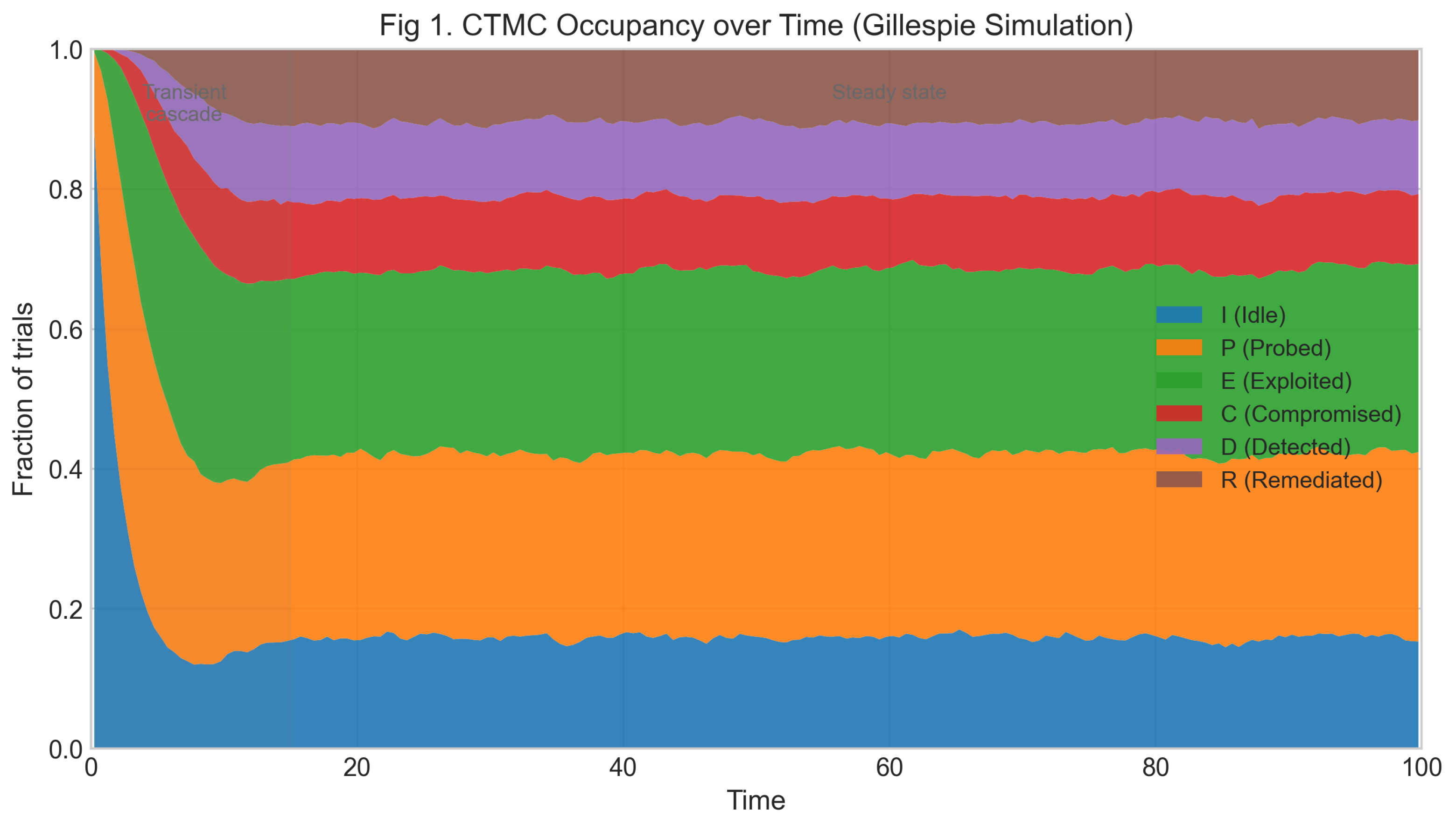
Figure 2.
Replicator phase portrait. The trajectory traces closed orbits around the mixed-strategy equilibrium , marked by the red star. The green dot marks the initial condition . The equilibrium is a center: Lyapunov stable but not asymptotically stable.
Figure 2.
Replicator phase portrait. The trajectory traces closed orbits around the mixed-strategy equilibrium , marked by the red star. The green dot marks the initial condition . The equilibrium is a center: Lyapunov stable but not asymptotically stable.
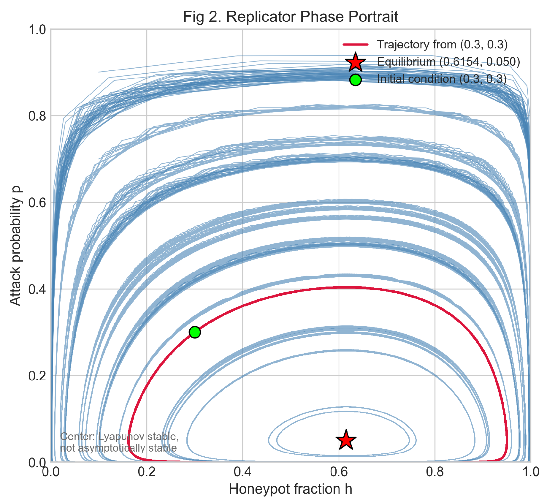
Figure 3.
Weibull detection-time distribution with shape and scale . The blue histogram shows Monte Carlo samples; the red curve is the theoretical pdf; the dashed vertical line marks the analytic mean .
Figure 3.
Weibull detection-time distribution with shape and scale . The blue histogram shows Monte Carlo samples; the red curve is the theoretical pdf; the dashed vertical line marks the analytic mean .
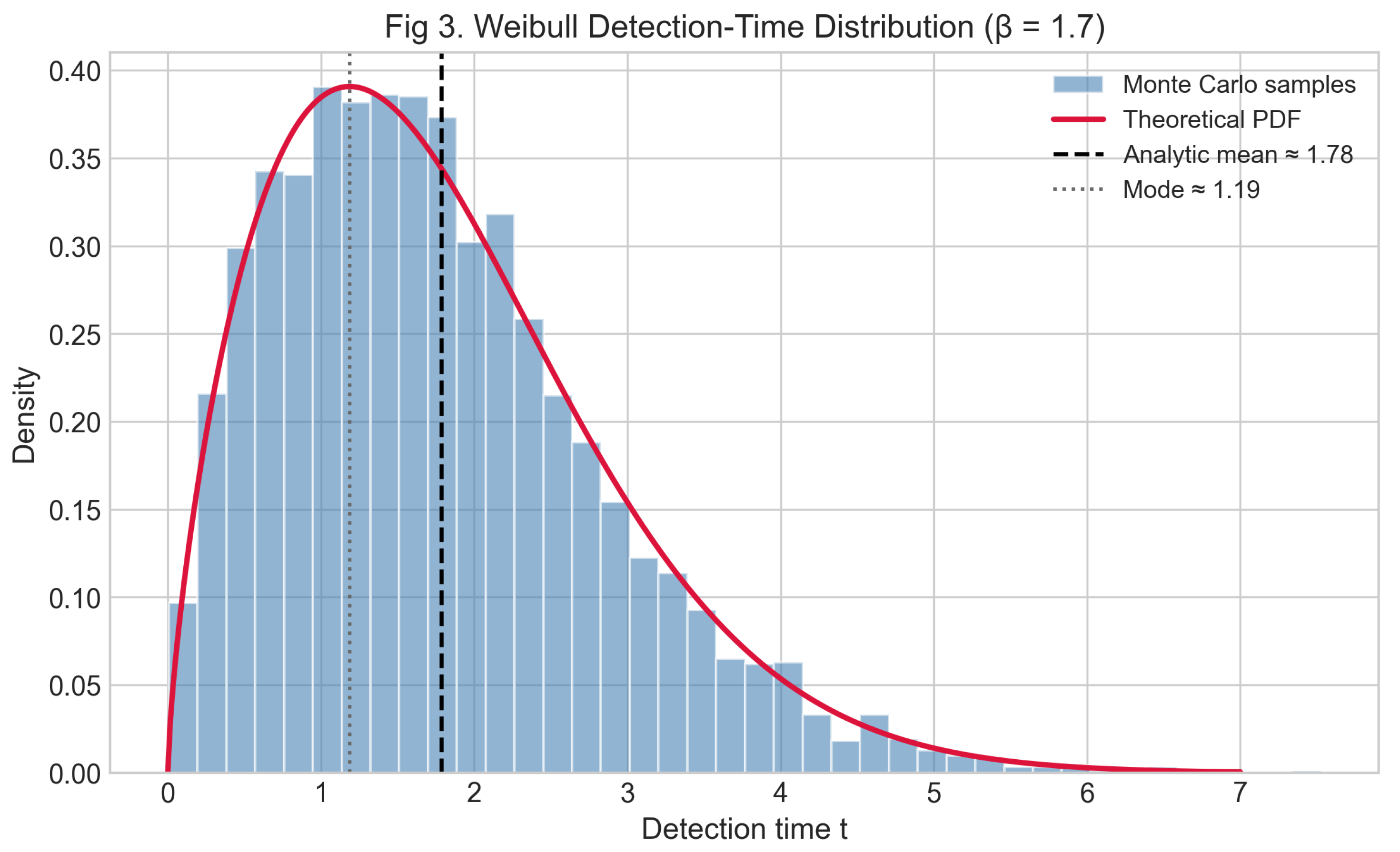
Figure 4.
Convergence of (Weibull) as a function of on a logarithmic x-axis. The blue line is the empirical mean; the shaded band is the confidence interval; the red dashed line is the analytic mean . The band narrows like .
Figure 4.
Convergence of (Weibull) as a function of on a logarithmic x-axis. The blue line is the empirical mean; the shaded band is the confidence interval; the red dashed line is the analytic mean . The band narrows like .
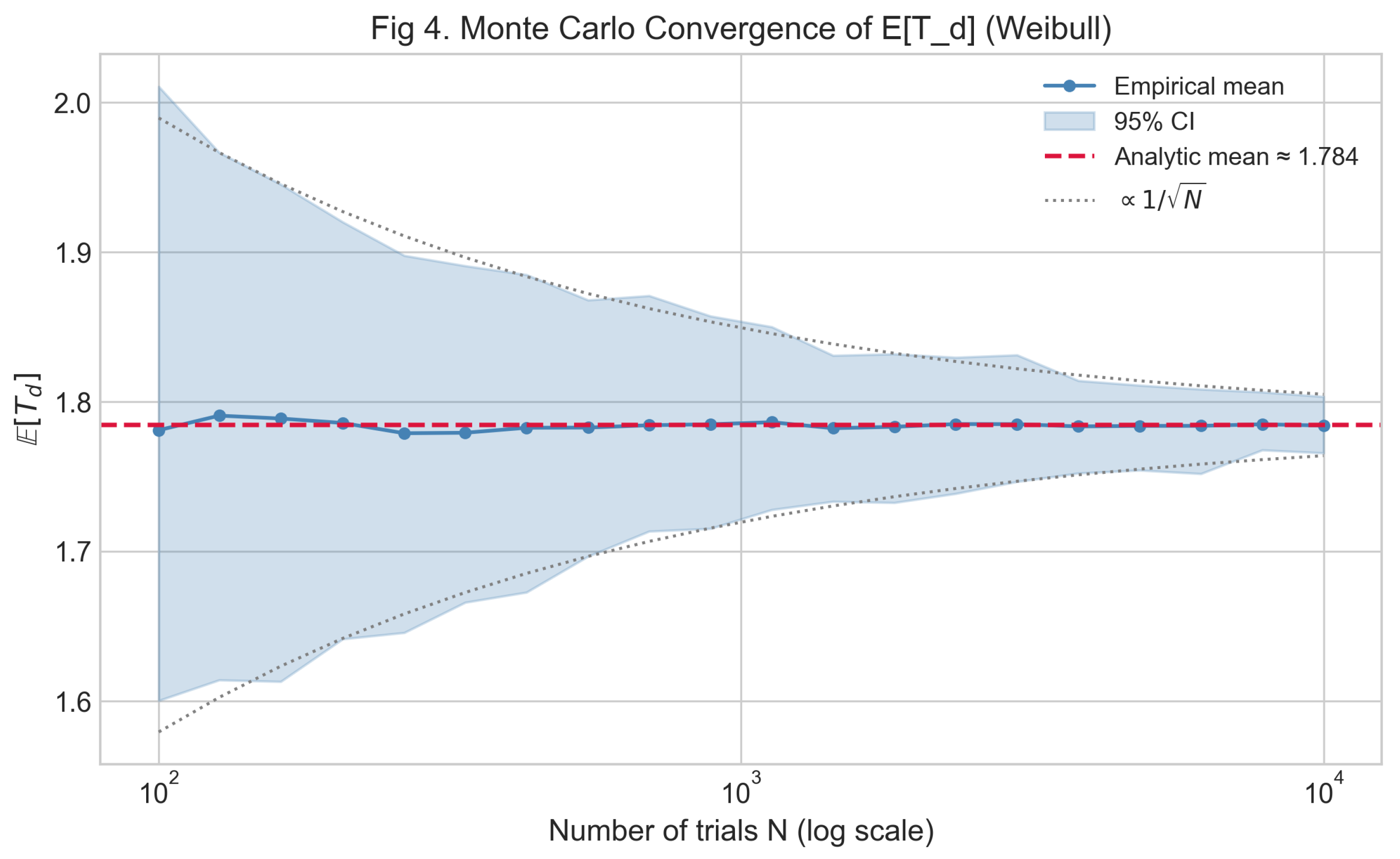
Figure 5.
Mutual information for a symmetric channel with inputs as a function of the error probability . The curve is U-shaped, with minimum near and equal values 1 bit at and .
Figure 5.
Mutual information for a symmetric channel with inputs as a function of the error probability . The curve is U-shaped, with minimum near and equal values 1 bit at and .
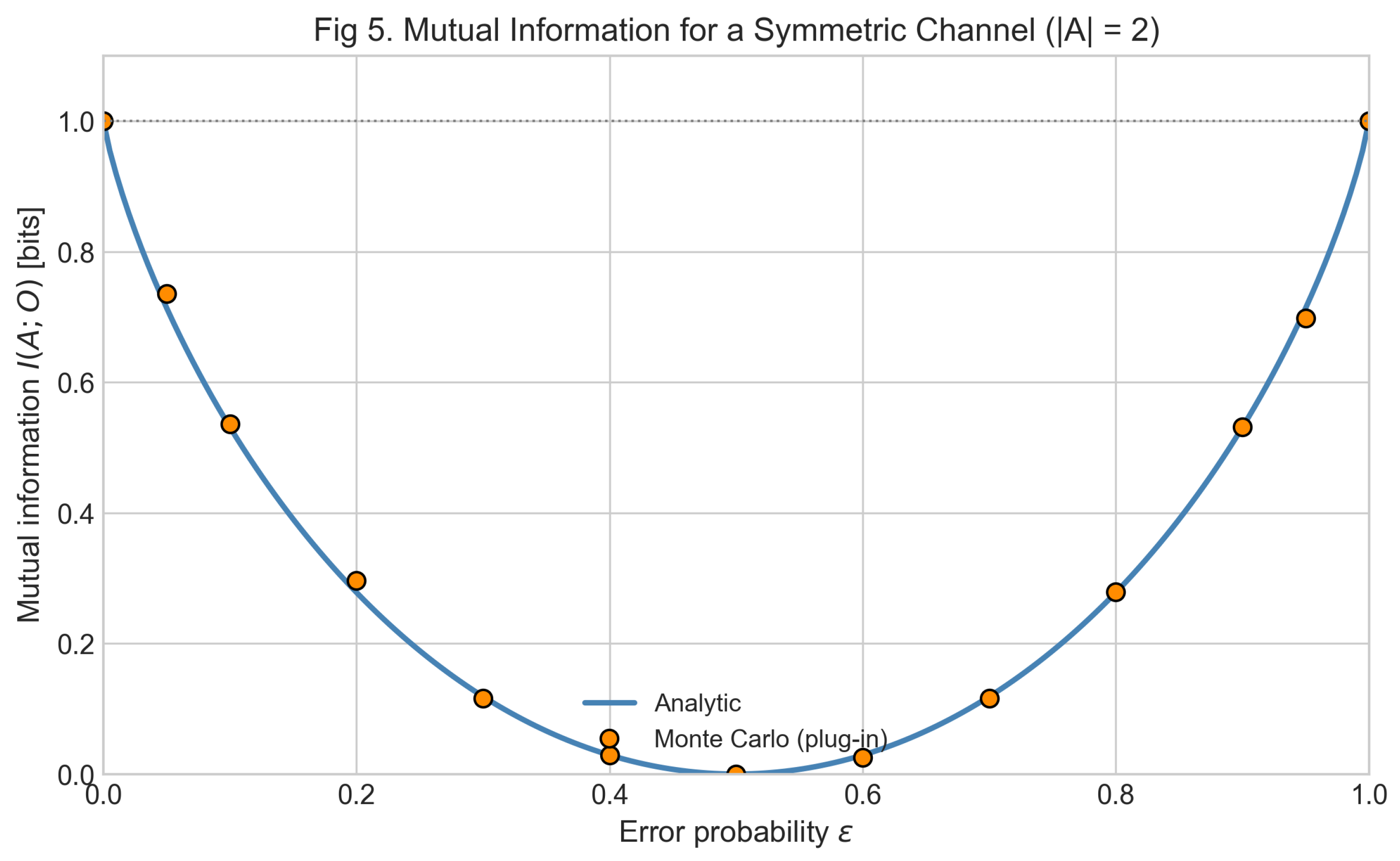
Figure 6.
Defender utility surface. The red star marks the equilibrium .
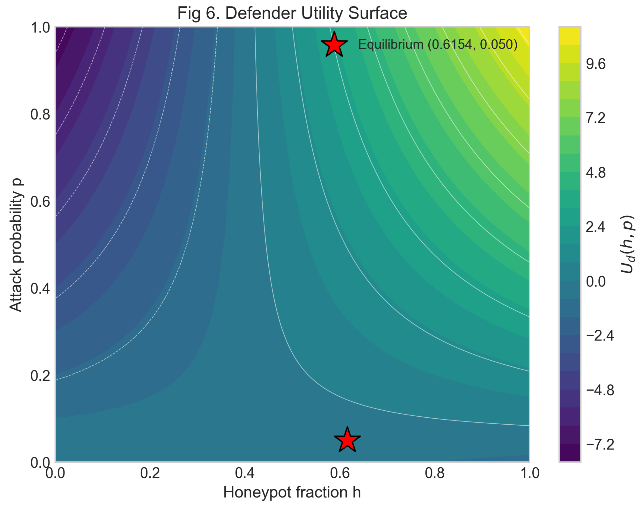
Table 4.
Summary of numerical findings. Every empirical estimate agrees with its analytic counterpart to within Monte Carlo error at .
Table 4.
Summary of numerical findings. Every empirical estimate agrees with its analytic counterpart to within Monte Carlo error at .
| Quantity | Analytic | Empirical | Rel. error | Source |
|---|---|---|---|---|
| (deterrence) | 0.6154 | — | — | Prop. 5.1 |
| (honeypot fraction) | 0.6154 | — | — | Prop. 5.2 |
| (attack prob.) | 0.0500 | — | — | Prop. 5.2 |
| 7.33 | 7.28 | 0.7% | Thm. 4.2 | |
| Poisson | 2.00 | 2.00 | 0.1% | Prop. 6.2 |
| Weibull () | 1.79 | 1.78 | 0.6% | Thm. 6.3 |
| Poisson | 16.0 | — | — | Prop. 6.2 |
| Weibull () | 14.3 | — | — | Thm. 6.3 |
| 0.9174 | 0.9165 | 0.1% | Prop. 6.1 | |
| at | 0.5310 | 0.5287 | 0.4% | Eq. (63) |
| at | 1.0000 | 0.9983 | 0.2% | Eq. (64) |
Disclaimer/Publisher’s Note: The statements, opinions and data contained in all publications are solely those of the individual author(s) and contributor(s) and not of MDPI and/or the editor(s). MDPI and/or the editor(s) disclaim responsibility for any injury to people or property resulting from any ideas, methods, instructions or products referred to in the content. |
© 2026 by the authors. Licensee MDPI, Basel, Switzerland. This article is an open access article distributed under the terms and conditions of the Creative Commons Attribution (CC BY) license (http://creativecommons.org/licenses/by/4.0/).
Copyright: This open access article is published under a Creative Commons CC BY 4.0 license, which permit the free download, distribution, and reuse, provided that the author and preprint are cited in any reuse.