

Submitted:
09 October 2026
Posted:
09 October 2026
You are already at the latest version
Abstract
Quantifying coastal spatial complexity across continuous display scales in digital mapping architectures is traditionally constrained by static raster resolution boundaries, quantization errors, and manual operator bias. Furthermore, dynamic web-mapping services deploy scale-dependent cartographic generalization, causing displayed geometries to reflect geospatial database complexity rather than static physical boundaries. To address these challenges, this study presents an automated, hybrid Web-GIS and MATLAB geospatial processing pipeline that integrates commercial web-mapping API vector-rendering engines with digital image processing to facilitate continuous multi-scale cartographic complexity (Db) benchmarking and feature extraction. By maintaining a constant physical-scale measuring grid—calibrated via a dimensionless coordinate-ratio parameter—over programmatically scaled vector cartography, the pipeline leverages sub-pixel geometric precision to achieve seamless multi-scale coastal feature extraction. The framework incorporates connected-component labeling (CCL) noise filtration, Otsu thresholding, Canny edge detection, Gecko-engine tile rendering to eliminate WebKit-induced stitching grid artifacts, and latitudinal scale-distortion compensation for Web Mercator projections. Deployed across 16 global geospatial databases, the pipeline demonstrates robust spatial benchmarking capabilities: along Norway's glaciated coastline (Db=1.4395), it effectively captures a scale-dependent, biphasic "fjord-to-fjard" morphometric transition, resolving spatial thresholds corresponding to meso-scale glacial valley morphometry. Global database benchmarking reveals clear structural distinctions in cartographic complexity, where active convergent boundaries exhibit elevated fractal complexity (e.g., Southeast Asia, Db=1.4578) compared to transform-suppressed margins (e.g., US West Coast, Db=1.0460). Additionally, a macro-scale cartographic low-pass filter (>0.8 km, Zoom 2–7) effectively attenuates high-frequency cartographic noise and anthropogenic structural inflation (e.g., 56.29% artificial coastlines in Taiwan). This open-source workflow provides a robust, reproducible Web-GIS framework for dynamic spatial database benchmarking, digital cartographic analysis, and automated coastal feature extraction.
Keywords:
web-GIS pipeline
; web-mapping APIs
; cartographic complexity
; box-counting fractal dimension
; digital cartography
; geospatial database benchmarking
; coastal feature extraction
; reproducible workflow
1. Introduction
Quantifying the morphological complexity of natural terrestrial-aquatic interfaces across continuous spatial scales represents a fundamental challenge in spatial informatics, digital cartography, and geographic information science (GIScience). Natural shorelines exhibit non-Euclidean, highly fragmented geometries that resist simplified parameterization via classical Euclidean metrics. This measurement challenge is epitomized by the “coastline paradox,” first documented empirically by L. F. Richardson [1] and subsequently formalized through fractal geometry by B. Mandelbrot [2,3], which demonstrates that the measured length of a natural shoreline continuously diverges as observation resolution increases. In modern geographic information systems (GIS), web mapping services, and spatial data infrastructures (SDIs) [4], evaluating continuous scale-dependent complexity is critical for environmental modeling, coastal hazard assessment, dynamic spatial database indexing, and automated feature extraction. However, traditional spatial analysis workflows remain constrained by static, resolution-limited raster databases, introducing severe pixelation boundaries, quantization errors, and subjective operator bias during multi-scale grid superpositions.
To parameterize these complex spatial structures, the box-counting fractal dimension (Db) has been widely integrated into spatial processing toolkits [3] and graphic complexity benchmarking models [5]. In classical GIS implementations, this method superimposes a series of grids with varying cell sizes over a static raster image, counts occupied cells, and extracts Db from the slope of a double-logarithmic regression line [6]. Despite its computational popularity, this traditional raster-based paradigm suffers from inherent technical limitations. Applying multi-scale grid overlays to a static raster file degrades spatial fidelity at high resolutions, because pixel-boundary artifacts artificially distort edge structures. Furthermore, manually selecting grid origins and bounding boxes introduces operator-induced variance, limiting the reproducibility of multi-scale geomorphometric assessments. Consequently, static raster pipelines struggle to resolve subtle, scale-dependent structural transitions without sampling artifacts.
A critical evaluation of traditional geomorphometry reveals a persistent mismatch between fixed-resolution datasets and the requirements of multi-scale observation. Conventional workflows rely heavily on discretized raster charts, where spatial downscaling inevitably induces pixelation and geometric blurring [7,8]. When analyzing digital cartographic interfaces, an additional computational consideration emerges: commercial web-mapping platforms deploy scale-dependent cartographic generalization algorithms—such as line simplification, feature selection, and dynamic tile smoothing—to optimize web rendering performance across zoom levels [9,10]. Consequently, multi-scale fractal dimensions extracted from digital web cartography reflect the cartographic complexity of the underlying geospatial database across variable representation scales, rather than an absolute, scale-invariant physical boundary. Establishing a rigorous spatial informatics pipeline therefore requires an automated framework that can process scale-independent vector geometries while explicitly controlling for cartographic rendering noise, web-tile stitching artifacts, and latitudinal projection distortions.
To overcome the resolution constraints and manual biases of static raster analysis, this study presents an automated, hybrid geospatial informatics pipeline that integrates commercial web-mapping API vector-rendering engines with MATLAB digital image processing. The proposed framework reverses the classical measurement paradigm: it maintains a constant physical-scale measuring grid on the display system—calibrated via a dimensionless coordinate-ratio parameter (g)—while programmatically scaling the underlying scale-independent vector map geometry across continuous cartographic zoom levels. To ensure computational rigor, the processing workflow incorporates a custom JSON API styling payload to isolate marine-terrestrial boundaries [11] for automated shoreline detection [12], leverages the Gecko rendering engine (Mozilla Firefox) to eliminate WebKit-induced tile-stitching grid artifacts, and applies Otsu binarization [13] with 8-connectivity connected-component labeling (CCL) [14] to filter out non-target geographic noise. High-precision Canny edge detection [15] subsequently extracts a topologically closed, single-pixel coastline, while a mathematical compensation model corrects for Web Mercator latitudinal scale distortion [16].
By deploying this dynamic multi-scale framework across global spatial databases, this study advances the fields of geospatial informatics and quantitative digital cartography in four primary aspects (Figure 1):
- Vector-Based Measurement Technique: We establish an open-source, reproducible spatial computation workflow that eliminates static raster pixelation boundaries and human operator bias by coupling web-mapping API vector engines with automated digital image processing.
- Scale-Dependent Geomorphic Dynamics: We demonstrate the scale-resolving capability of the pipeline along the glaciated Norwegian coastline (Db = 1.4395), capturing a non-linear, biphasic “fjord-to-fjard” structural transition and resolving spatial scale thresholds matching meso-scale glacial valley morphometry.
- Global Cartographic Benchmarking: We compile a systematic spatial benchmark across 16 global coastal regions, demonstrating that regional cartographic complexity aligns with macro-scale tectonic regimes. Active convergent margins (e.g., Southeast Asia, Db = 1.4578) exhibit elevated fractal ruggedness due to intense crustal deformation, whereas transform faults (e.g., US West Coast, Db = 1.0460) and passive margins display structurally suppressed, low-complexity profiles.
- Macro-Scale Spatial Low-Pass Filtering: We evaluate applying a macro-scale spatial low-pass filter (>0.8 km, Zoom 2 to 7) within the digital image processing workflow. This filtering framework effectively attenuates high-frequency modern cartographic noise (e.g., localized wave erosion, anthropogenic harbor structures, and micro-scale coastal complexity), isolating stable macro-scale structural features across broad geographic domains and providing a robust spatial processing window for multi-scale database analysis.
The remainder of this paper is organized as follows: Section 2 details the four-stage automated geospatial informatics methodology, including web-API vector acquisition, MATLAB digital image processing, latitudinal scale compensation, and double-logarithmic regression parameters. Section 3 presents the empirical spatial results, validating the pipeline across baseline endmembers, resolving the scale-dependent Norwegian “fjord-to-fjard” transition, and establishing a global cartographic complexity benchmark across 16 regions. Section 4 discusses the technical advantages of sub-pixel vector processing, evaluates scale sensitivity against anthropogenic noise, and contextualizes macroscopic transform-margin features. Finally, Section 5 concludes the paper and summarizes the open-source software contribution.
2. Materials and Methods
To systematically overcome the scale-dependent resolution degradation, quantization errors, and subjective operator bias in traditional static raster-based geomorphological mapping, this study implements an automated, hybrid geospatial informatics pipeline. The proposed methodology reverses the traditional measurement paradigm by maintaining a constant physical-scale measuring grid on the display architecture—calibrated via a dimensionless coordinate-ratio parameter (g)—while dynamically scaling the underlying scale-independent vector cartography across continuous cartographic zoom levels. This dynamic box-counting framework ensures absolute geometric fidelity across an unprecedented macro-to-micro spatial spectrum, extracting the scale-dependent cartographic complexity of digital geospatial databases (schematically illustrated in Figure 2). For a holistic structural overview of the automated four-step spatial informatics pipeline, see Supplementary Figure S1. The complete computational workflow is deployed in MATLAB and executed through four integrated protocols as detailed below.
2.1. Step 1: Scale-Independent Cartographic Data Acquisition and API Customization
The first phase of the pipeline compiles pristine, ultra-high-resolution spatial datasets that preserve geographical features without pixelation artifacts during scaling. Unlike static GIS raster charts, this framework leverages the vector rendering engine of the commercial Google Maps JavaScript API [9], which mathematically formulates geographical boundaries as continuous vector layers. To isolate the marine-terrestrial interface, we programmatically manipulate the API’s vector-drawing layers by injecting custom JSON style declarations [11]. This payload systematically suppresses administrative borders, cartographic annotations, transit lines, and cultural features (points of interest), while optimizing radiometric contrast by mapping landmasses and water bodies to highly distinct, uniform hexadecimals (Figure 2a).
To acquire massive cartographic tiles, we utilize an automated coordinate-based screen-capture utility, MapCapt, which stitches seamless high-resolution images of up to 100 megapixels (10,000 × 10,000 pixels). Crucially, empirical calibration requires executing this acquisition process exclusively in Mozilla Firefox (Gecko rendering engine). As shown in Supplementary Figure S2, WebKit-based browsers (such as Google Chrome and Apple Safari) introduce latent, single-pixel tile-boundary coordinate grid lines during canvas stitching. These rendering artifacts trigger catastrophic false positives during automated edge detection. In contrast, the Gecko rendering engine successfully suppresses these stitching lines, guaranteeing a pristine, artifact-free dataset for subsequent processing.
2.2. Step 2: Digital Image Processing, CCL Noise Filtration, and Precise Edge Detection
The compiled high-resolution canvases are processed within a standardized MATLAB digital image processing pipeline to extract a mathematically continuous, closed, and single-pixel-wide coastline boundary. The workflow comprises four sequential sub-protocols (schematically detailed in Figure 2b and Supplementary Figure S3):
- Grayscale Conversion and Contrast Optimization: The raw multi-channel RGB image is converted into a single-channel grayscale matrix. Contrast-Limited Adaptive Histogram Equalization (CLAHE, via MATLAB’s adapthisteq operator) is executed to locally optimize intensity gradients across the full spectrum. This process normalizes localized illumination disparities, maximizing the radiometric gradient at the land-water boundary.
- Automated Binary Segmentation: Using Otsu’s global thresholding method (graythresh) [13], the normalized grayscale image is segmented into a binary matrix. In this binary mask, terrestrial landmass pixels are assigned a logical value of 1 (rendered white) and oceanic water bodies are assigned a logical value of 0 (rendered black).
- Connected-Component Labeling (CCL) Spatial Noise Filtration: To ensure mainland structural continuity, an 8-connectivity connected-component labeling (CCL) scheme [14] is first applied to filter out isolated offshore noise and minor islets. Next, the imfill operator programmatically removes the internal topological holes representing inland lakes, ensuring the edge-detection algorithm focuses exclusively on the primary marine-terrestrial interface. The algorithm evaluates disconnected inland water bodies, minor offshore islands, and localized screen-capture noise based on their relative pixel area. To prevent artificial inflation of the box count, any isolated component constituting less than 0.1% of the primary mainland’s total area is programmatically classified as geographic noise and deleted (reassigned to 0) in the binary mask.
- Precise Coastline Edge Delineation: To extract the continuous, unfragmented boundary contour, we execute the multi-stage Canny edge-detection operator [15]. Unlike traditional first-order gradient operators (such as Sobel or Prewitt), which produce coarse, multi-pixel-wide borders, the Canny operator implements sequential Gaussian smoothing, gradient search, non-maximum suppression, and hysteresis thresholding. This ensures a topologically closed, single-pixel-wide coastline boundary that preserves absolute geometric fidelity for the next grid-counting phase.
2.3. Step 3: Mathematical Formulation of the Dynamic Grid Scaling Framework and Latitudinal Compensation
Rather than programmatically resizing grid overlays over a static, resolution-limited raster image—which degrades the statistical scaling law due to pixelation—our methodology maintains a constant physical-scale measuring grid on the display system while programmatically scaling the underlying scale-independent vector map geometry (Figure 2c). To maintain spatial consistency across global regions, the algorithm must compensate for the severe latitudinal scale distortion introduced by the Web Mercator projection [16]. At any specific geodetic latitude θ and zoom level n, the instantaneous spatial resolution (meters per screen pixel) is mathematically formulated as:
where S0≈156,543.03 m/pixel represents the equatorial resolution baseline at zoom level 0. Accordingly, for a superimposed physical sampling grid characterized by a constant physical box side length Wgrid on the display system, the equivalent physical ground-truth scale ϵn,θ (meters) is dynamically calibrated across the multi-scale spectrum as:
In this formulation, the parameter g (pixels/cell) serves as a dimensionless coordinate ratio, mapping the physical grid geometry into the raster processing workspace. Under our experimental setup, the superimposed physical grid is calibrated to maintain an absolute constant spatial density of ρgrid = 40.25 cells/cm on the screen. This density establishes a highly macroscopic, human-resolvable grid box side length of Wgrid = 10/ρgrid≈0.2484 mm, which is completely free from physical display rendering limitations or optical diffraction constraints. Given the physical pixel pitch of the calibrated LCD monitor (pm≈0.3073 mm/pixel), the dimensionless coordinate ratio g is mathematically derived as the ratio of these two macroscopic physical dimensions:
By applying this calibrated value of g to Eq. (2), at a mean geodetic latitude of θ = 24° (Taiwan) and an exemplary zoom level of n = 6, the equivalent physical grid box size is calibrated to ϵ = 1.8066 km. This corresponds to a cartographic display scale of 72.72 km/cm at n = 6, where 1.8066 km/cell ×40.25 cells/cm ≈72.72 km/cm. In the MATLAB environment, the box-counting algorithm automatically overlays this calibrated virtual grid, scans the single-pixel binary coastline contour, and aggregates the total number of occupied grid cells N(ϵ) for each zoom level n, systematically generating a high-precision multi-scale dataset. Supplementary Figure S4 schematically details the algorithmic execution of this dynamic grid-counting loop and the geodetic scale calibration across sequential zoom levels.
It is worth noting that while the dimensionless coordinate-ratio parameter g is mathematically less than unity (g≈0.8085 pixels/cell), the physical sampling grid itself remains highly macroscopic (Wgrid≈0.2484 mm), thereby completely bypassing any physical display or optical resolution limits of the LCD system. Within the computational workspace, because the web-mapping API renders coastline boundaries with sub-pixel floating-point vector precision rather than discrete integer raster constraints, the fractional scaling value of g does not trigger coordinate overlap or grid-counting degeneracy. To ensure absolute methodological rigor across all scaling spectra, the MATLAB processing engine integrates an automated “Sub-Pixel Security Guard” protocol (detailed in Section S1.3). This system dynamically verifies that the equivalent ground-truth scale ϵ at high zoom levels remains larger than the rendering canvas’s minimum resolvable vector limit, ensuring that the OLS regression runs only within valid geomorphological power-law windows.
2.4. Step 4: Theoretical Scaling Laws, Double-Logarithmic Regression, and Scale-Filtering Windows
The mathematical extraction of the coastal fractal dimension relies on quantifying the scale-dependent power-law relationship embedded within the multi-scale dataset. For a natural coastline exhibiting statistical self-similarity across a discrete spectrum of physical scale factors ϵ, the relationship between the cumulative count of intersected grid cells N(ϵ) and the physical scale ϵ is formulated as:
where Db denotes the box-counting fractal dimension. To linearize this exponential power law for rigorous statistical estimation, a double-logarithmic transformation is executed in MATLAB, mapping the dataset onto a two-dimensional Cartesian coordinate system:
where C represents a constant scaling coefficient. A linear least-squares regression model computes the best-fit line by minimizing the sum of squared residuals. The slope m of this optimized linear equation directly yields the bulk fractal dimension Db. Supplementary Figure S5 shows a graphical demonstration of the OLS double-logarithmic regression and slope extraction for representative high- and low-complexity endmembers. Under practical measurement conditions, however, the fractal dimension is not a constant value but varies with the measurement scale ϵ. From Eq. (5), the dynamic scale-dependent value of Db(ϵ) is evaluated as:
In our dynamic scaling framework, the variation in physical scale ∆ϵ is driven solely by the discrete increment in zoom level n (such that ∆n = 1 between adjacent levels n and n − 1). Utilizing the physical scale relation in Eq. (2), we obtain ∆(log(1/ϵ)) = (log2)∆n. Substituting this relationship into Eq. (6) yields the instantaneous fractal dimension determined by zoom level n:
To ensure the statistical validity of the extracted dimensions, the regression pipeline automatically compiles a suite of diagnostics, enabling targeted scale filtering by customizing the fitting window boundaries:
- Baseline Validation Window: For localized self-similarity analyses (such as Taiwan, Great Britain, and Norway), the regression is executed across the entire acquired scale spectrum (typically Zoom 2 to 17) to capture full, multi-scale scaling dynamics.
- Macro-Scale Cartographic Window: For global-scale spatial database benchmarking, the fitting window is restricted to Zoom levels 2 to 7 (ϵ > 0.8 km). This scale filtering effectively attenuates modern high-frequency noise and captures stable macro-scale boundary geometries.
- Statistical Quality Control: The regression pipeline computes the coefficient of determination (R²) to quantify the goodness-of-fit and verify power-law consistency. The standard error of the estimate is calculated to provide confidence intervals for Db, and residual variance analysis is automatically performed. Non-linear, systematic deviations in residual plots serve as crucial indicators of scale-dependent geomorphological transitions, such as the Norwegian ‘fjord-to-fjard’ structural shift.
3. Empirical Results and Spatial Analysis
3.1. Methodological Validation, Baseline Self-Similarity, and Hemispheric Disparities
To evaluate the mathematical validity and operational robustness of the automated hybrid geospatial informatics pipeline, we ran initial baseline measurements along the coastlines of Taiwan, Great Britain, and Norway. We selected these geographic domains to represent low-, intermediate-, and high-structural-complexity endmembers within our global geomorphological database. Figure 3 quantitatively compared the multi-scale scaling trajectories and extracted bulk fractal dimensions (Db) of these three representative geographies. Double-logarithmic regression analyses performed on the multi-scale datasets confirm the inherent statistical self-similarity and power-law scaling consistency of natural shoreline geometries. The empirical results show that distinct regional geomorphic histories govern spatial scaling behavior, yielding stable fractal metrics across broad spatial resolution spectra.
For Great Britain, the classic benchmark of the coastline paradox, the pipeline processed the contiguous shoreline across ten discrete cartographic zoom levels (Zoom 3 to Zoom 12). This resolution interval extends from a macro-scale to a detailed sub-kilometer resolution, culminating in 1,077,727 occupied grid cells at Zoom 12. Linear least-squares regression of the double-logarithmic dataset yields a highly robust scaling law governed by the empirical equation logN(ϵ) = 1.1858log(1/ϵ) + 2.8305, with a coefficient of determination R2 exceeding 0.99. This extracted bulk fractal dimension Db = 1.1858 mathematically validates the structural irregularity originally investigated in seminal manual geomorphometric studies. Supplementary Figure S8 illustrates the OLS double-logarithmic regression and the subtle downward micro-scale scaling trend characterizing this natural reference baseline. In contrast, Taiwan’s coastline shows the lowest overall complexity in our validation suite, yielding a bulk fractal dimension of Db = 1.0958 across twelve spatial scales (Zoom 6 to Zoom 17), representing a physical span from 72.72 km/cm down to 35.5 m/cm. At the maximum zoom level (Zoom 17), the pipeline successfully evaluated 4,974,657 occupied grid boxes. This low dimension is geomorphologically driven by the smooth western alluvial plains and sandy deltaic systems along Taiwan’s coast.
At the high-complexity extreme, Norway’s highly fragmented glaciated coastline yields a remarkably elevated bulk fractal dimension of Db = 1.4395 across eight Zoom levels (Zoom 4 to Zoom 11), with occupied grid boxes expanding exponentially from 1,753 at Zoom 4 to approximately 1.89 million at Zoom 11. The resulting linear regression equation is established as logN(ϵ) = 1.4395log(1/ϵ) + 2.8558. Comparing the multi-scale grid counts of Great Britain and Norway reveals a crucial scaling phenomenon: while their log-transformed occupied grid counts converge at macro-scales (Zoom 4), they diverge by nearly an order of magnitude at Zoom 11. This divergence underscores how structural complexity compounds exponentially as spatial resolution increases, experimentally confirming the need for a scale-independent computational workflow.
On a global planetary scale, our integrated assessment establishes a baseline average coastline fractal dimension of Db = 1.416. Programmatic partitioning of the terrestrial-aquatic boundary along the equatorial plane (θ = 0°) reveals a pronounced hemispheric structural divergence. The Northern Hemisphere exhibits significantly elevated geometric ruggedness (Db,North = 1.3835), whereas the Southern Hemisphere presents a smoother, lower-stress profile (Db,South = 1.2990). This structural asymmetry is geomorphologically driven by two primary factors:
- Terrestrial Mass Allocation: Continental crust distribution is heavily skewed, with the Northern Hemisphere encompassing approximately 67.3% of global continental landmass compared to 32.7% in the Southern Hemisphere, amplifying boundary folding and accretion.
- Glacio-Geomorphic Fingerprints: Quaternary glacial footprints are heavily concentrated in high northern latitudes. The extensive fjord, skerry, and archipelago systems of Canada, Greenland, and Northern Europe act as high-frequency boundary distributors, shifting the Northern Hemispheric scaling trajectory toward a higher-dimensional topological attractor [17,18,19].
Supplementary Figure S9 provides comparative visualizations of these global and hemispheric coastal fractal baselines and their respective power-law scaling trajectories.
3.2. Scale-Dependent Geomorphological Transitions and Glacial Constraints
A critical finding of our multi-scale framework is that the fractal dimension Db is not a static constant, but a dynamic, scale-sensitive geomorphic indicator that captures non-linear transitions. In Taiwan, localized scaling window analysis reveals a distinct biphasic trend. At intermediate scales (Zoom 6 to 9), the coastline displays a highly smooth, structurally suppressed fractal dimension of 1.0227, reflecting the natural monotonicity of the western alluvial plains. However, as magnification increases toward micro-scales (Zoom 14 to 17), the calculated dimension escalates sharply to 1.1713, closely approaching the bulk complexity of Great Britain’s natural coastline. This resurgent complexity is synthetically inflated by extensive anthropogenic coastal armoring. Specifically, concrete tetrapods, seawalls, and port infrastructure occupy 56.29% of Taiwan’s shoreline. Under high-resolution Web-API rendering, these blocky, highly fragmented artificial structures introduce high-frequency geometric noise that dominates the geomorphic signal at sub-meter scales.
Conversely, Great Britain’s natural coastline shows a minor downward trend at micro-scales, reflecting a gradual geometric generalization free from anthropogenic synthetic inflation. This finding demonstrates that high-resolution geospatial informatics pipelines must incorporate land-use and anthropogenic filters to prevent artificial structures from confounding natural geomorphological complexity metrics. Supplementary Figure S6 plots the full spatial scaling spectrum and the pronounced, anthropogenically inflated biphasic transition of Taiwan’s coastline.
Norway’s glaciated coastline exemplifies a highly irregular geomorphic system governed by scale-dependent glacial constraints, revealing a distinct “fjord anomaly.” Within the meso-scale bandwidth of Zoom 4 to 7 (corresponding to physical grid edge lengths ϵ between 4 km and 500 m), Norway’s calculated fractal dimension surges to a localized peak of Db = 1.5167. This result shows high empirical consistency with physicist Jens Feder’s classic calculation of Db = 1.52 across scales of 80 km to 600 m [20], confirming that the peak of Norway’s structural ruggedness is heavily concentrated within this spatial band. However, as the measurement scale drops below the 500 m threshold (Zoom 6 to 9), the calculated fractal dimension experiences a transient structural depreciation, contradicting the conventional assumption of monotonic multi-scale ruggedness. This localized geometric simplification is physically restricted by the U-shaped morphometry of glacial valleys. Glaciers, operating as high-pressure flowing solids that slide and carve bedrock once snow accumulation reaches a critical thickness (~30 m), carve U-shaped valleys with a characteristic depth-to-width ratio of approximately 0.45 [21,22]. This ratio sets a minimum basal-width threshold [23], causing the calculated fractal dimension to decline when the measurement unit falls below this physical boundary limit.
At ultra-high magnifications (Zoom 8 to 11), Norway’s calculated fractal dimension resumes an increasing trend, representing a structural resurgence. This micro-scale rebound is geomorphologically driven by the emergence of “fjards”, the glaciated lowlands situated at the seaward outlets of fjord networks. Unlike the deeply incised, U-shaped glacial valleys that dominate meso-scales, these seaward fjards feature highly irregular, shallow, and chaotic geomorphic profiles. As the upstream fjord networks become generalized under high magnification, these intricate lowland structures begin to dominate the system’s geometric signal, confirming a scale-dependent, non-linear fjord-to-fjard structural transition. Refer to Supplementary Figure S7 for the complete empirical spatial spectrum, the localized ‘fjord anomaly,’ and the physical glacial valley morphometric constraint models of the Norwegian coastline.
3.3. Global Lithospheric Controls and Structural Coastal Complexity
To isolate deep-seated, tectonic-scale lithospheric signatures from high-latitude glacio-geomorphic overprints, we constrained the multi-scale fractal analysis to global coastlines situated between latitudes 60°N and 60°S. Across this geographical band, we evaluated regional fractal dimensions at spatial scales from Zoom 1 to 5 across 16 distinct local regions. Under the Zoom 5 resolution baseline, the Web Mercator projection translates to a physical grid-box side length of approximately 2 km at 60° latitude and 3.6 km at 24° latitude. This spatial scaling acts as an effective high-frequency spatial filter (> 2 km), suppressing modern localized erosional and anthropogenic noise (such as wave-induced spit migration, beach accretion, and harbor construction) and preserving macroscopic, crustal-scale coastal geometry against the global baseline (Figure 4). While the spatial distribution across these 16 subdivisions is mapped in Figure 4, their multi-scale scaling behaviors and comprehensive regional taxonomy are quantitatively summarized in Supplementary Figure S10.
Our global regional assessment resolves profound disparities in coastal complexity, demonstrating a robust, first-order correlation between regional fractal dimensions and macroscopic tectonic drivers. The empirical datasets bifurcate into two statistically distinct geodynamical groups:
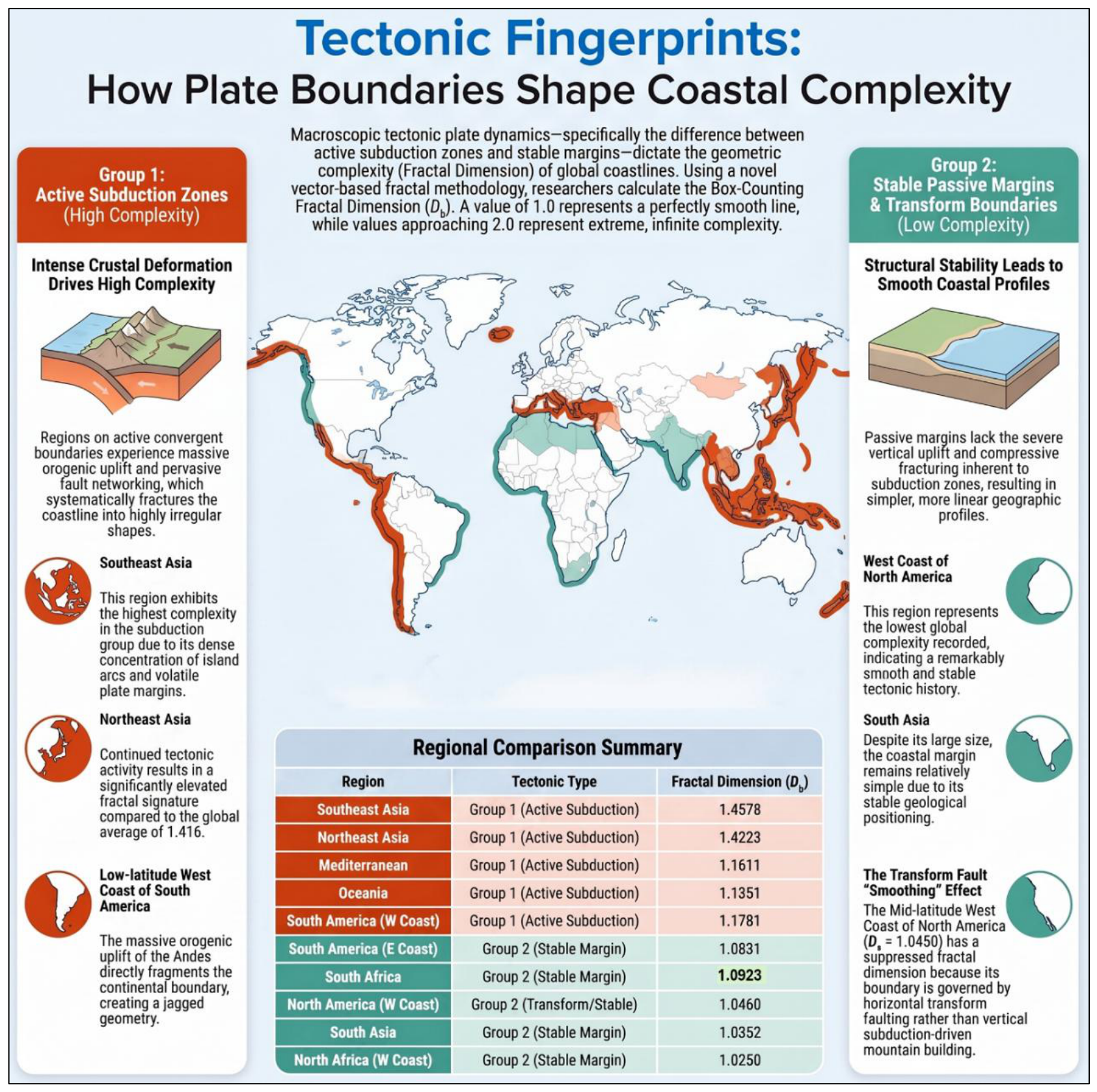
- Group 1: Active Convergent Margins and Orogenic Complexity Amplification. This group encompasses regional coastlines situated along active plate boundaries, primarily dominated by convergent subduction zones and multi-plate collisional interfaces. The continuous subduction of denser oceanic lithosphere drives intense compressive stress fields, continuous crustal deformation, rapid vertical orogenic uplift, and dense fault-propagation folding. These forcing mechanisms systematically segment and shatter the terrestrial boundary, producing highly rugged, fragmented, and irregular coastal profiles with elevated fractal dimensions (Db≫1.1) [24]. Southeast Asia exhibits the highest geometric complexity globally within the subglacial dataset (Db = 1.4578), driven by active island-arc accretion and multi-directional subduction. This is followed by Northeast Asia (Db = 1.4223), the Mediterranean collision interface (Db = 1.3466), and Oceania (Db = 1.2501). Similarly, the active Pacific convergent subduction margin of low-latitude South America yields Db = 1.1781, driven by Andean orogenesis.
- Group 2: Structurally Suppressed and Transform Boundaries. This category consists of stable passive continental margins governed by prolonged thermal subsidence, or regions dominated by strike-slip transform boundaries. Lacking compressive stress fields and severe vertical displacement, these coastlines are shaped by long-term subaerial weathering and wave-induced marine planation, tending toward highly linear, low-stress geomorphological baselines [18]. The West Coast of North Africa registers the lowest complexity within the global dataset (Db = 1.0250), closely aligned with stable cratonic margins in South Asia (Db = 1.0352) and South Africa (Db = 1.0923). Notably, the Mid-latitude West Coast of North America exhibits a suppressed Db of 1.046. Although situated along an active plate boundary, this Pacific margin is dominated by horizontal strike-slip transform tectonics (e.g., the San Andreas fault system). Because it lacks the compressive fracturing and severe vertical uplift characteristic of subduction zones, lateral displacement does not generate high-frequency coastal ruggedness, producing a smoother profile than its passive eastern counterpart (Db = 1.0872) [24]. This transform-boundary scenario demonstrates that lithospheric displacement styles act as a first-order control on structural complexity (schematically conceptualized in Figure 5). Supplementary Figure S11 shows a detailed transcontinental comparative analysis of coastal complexity across the Americas—encompassing glaciated Patagonia, low-latitude active subduction, and the transform-suppressed western margin.
4. Discussion
4.1. Methodological Rigor and the Web-API Rendering Paradox
The proposed geospatial informatics pipeline’s core technical advancement is its ability to resolve the historical trade-off between scale range and operator subjectivity in multi-scale box-counting fractal analyses [2,3]. Conventional approaches have traditionally superimposed dynamic grids on static, resolution-limited raster images, resulting in severe quantization artifacts and loss of geometric fidelity at high magnification levels [7]. By reversing this dynamic—maintaining a static pixel-size measuring grid while programmatically scaling the underlying map vector geometries through commercial Web-mapping APIs—the pipeline achieves a continuous multi-scale characterization from macro-geography (~1,000 km) to micro-structures (~50 m). However, this dynamic scaling approach introduces an inherent technical paradox: while the Web-mapping API renders geometries on the fly using underlying vector databases, the computational environment must capture these elements onto high-resolution rasterized canvases for subsequent digital image processing. Thus, our pipeline is a hybrid vector-rendering and raster-processing computational framework.
This hybrid nature necessitates a rigorous discussion of cartographic generalization and parameter sensitivity, which have historically been underreported in commercial API-based spatial models. Commercial mapping APIs (such as Google Maps) employ proprietary, scale-dependent generalization algorithms—including Douglas-Peucker line simplification, feature selection, and local projection adjustments—to optimize visual rendering at different zoom levels [10]. Consequently, the coastline geometry displayed at Zoom level n is not a mathematically identical scaling of Zoom n − 1, but a simplified, cartographically curated representation. The fractal dimension Db extracted by our algorithm is therefore a quantitative index of the cartographic complexity of the digitized geospatial database, rather than an absolute, scale-invariant physical coastline.
Furthermore, the extracted Db is highly sensitive to the parameters of the digital image processing step, particularly the hysteresis thresholds of the Canny edge detector and the binarization segmentation thresholds. In our MATLAB implementation, we held these parameters constant across all zoom levels to eliminate intra-analysis variance, but future informatics studies should incorporate systematic sensitivity analyses to quantify the exact mathematical influence of edge-thresholding parameters on global geomorphological classification.
4.2. Geomorphological Scale Sensitivity and Anthropogenic Inflation
The pipeline’s scale-resolving capability is clearly demonstrated by the biphasic scaling behavior observed along the Norwegian coastline. Traditional single-scale analyses often yield a static Db that obscures local scaling transitions. In contrast, our dynamic framework captures a distinct ‘dip’ in the localized fractal dimension Db(n) at intermediate spatial scales, followed by a robust geometric recovery. This biphasic pattern represents a physical geomorphological transition from macro-scale tectonic fjords to micro-scale islands and ‘fjards’ (glaciated lowlands). At meso-scales (4 km to 500 m, corresponding to Zoom levels 4 to 7), the coastline’s geometric complexity is dominated by deep, parallel glacial valleys whose width-to-depth ratios are physically bounded by ancient glacial erosion patterns. This produces a highly rugged, self-similar geometry with a peak Db of 1.5167, aligning precisely with the classic fractal models of Jens Feder [20]. At micro-scales (below 500 m), the measuring grid penetrates the interior of these glacial troughs, where the steep, near-linear granite cliffs present simplified, Euclidean profiles that cause a temporary drop in Db(n). This geometric ‘suppression’ is only broken at high magnifications (Zoom levels 8 to 11), where the algorithm begins resolving the complex, low-relief island systems and skerry guards (fjards) typical of post-glacial shorelines, triggering a second phase of fractal complexity.
Conversely, our analysis of the Taiwanese coastline highlights a critical phenomenon of ‘artificial scaling inflation’ in modern GIS datasets. At macro-to-meso scales, Taiwan exhibits a moderately smooth geomorphic baseline. However, at micro-spatial scales (Zoom levels 14 to 17, corresponding to physical grid sizes under 10 m), the localized Db experiences an anomalous, steep upward trajectory, peaking at 1.1713. While a purely mathematical interpretation might attribute this to high-frequency natural ruggedness, geomorphological ground-truthing reveals this as an artifact of extensive anthropogenic modifications. Currently, approximately 56.29% of Taiwan’s coastline is heavily artificialized with harbors, dykes, and massive concrete tetrapods designed for coastal defense. At sub-10 m resolutions, the Canny detector resolves the high-contrast, tessellated geometries of these concrete arrays as highly dense, multi-directional edge fragments. This artificial complexity inflates the box-counting occupancy N(ϵ), resulting in an artificially elevated Db. This finding demonstrates that high-resolution geospatial informatics pipelines must incorporate land-use and anthropogenic filters to prevent artificial structures from confounding natural geomorphological complexity metrics.
4.3. Macroscopic Cartographic Complexity and Transform Margin Features
By compiling a systematic, spatial benchmarking across 16 diverse global regions, this study establishes a robust statistical association between macroscopic plate boundary regimes and coastal fractal complexity. Active convergent boundaries, such as the active subduction zones of Southeast Asia (Db = 1.4578) and Northeast Asia (Db = 1.4223), consistently exhibit the highest fractal dimensions globally, second only to glaciated fjord systems. The intense compressive stress, vertical orogenesis, volcanism, and rapid tectonic uplift characteristic of convergent margins continuously generate high-frequency coastal fragmentation, multiple offshore barrier islands, and complex embayments. In stark contrast, stable passive margins, such as the Atlantic coast of North Africa (Db = 1.0250) and South Asia (Db = 1.0352), exhibit extremely low, near-Euclidean fractal dimensions. These stable, sediment-rich margins are dominated by long-term deltaic deposition, wave-action smoothing, and coastal progradation, which systematically suppress high-frequency geometric irregularities.
Intriguingly, our global taxonomy uncovers what we define as the ‘Transform Suppression Paradox’ along strike-slip plate boundaries. The Pacific coast of the United States (US West Coast), which is dominated by the San Andreas active transform fault system, exhibits a remarkably low fractal dimension (Db = 1.0460). From a conventional geomorphic perspective, active tectonic margins are expected to display high complexity. However, the strike-slip motion along transform faults is predominantly horizontal, resulting in lateral displacement with minimal vertical crustal deformation or folding. This strike-slip kinematic regime produces highly linear, parallel coastal ranges and straight, fault-controlled shorelines with virtually no major embayments or complex island systems. Consequently, despite being an active plate margin, its fractal complexity is severely suppressed, producing a profile smoother than even the stable passive margin of the US East Coast (Db = 1.0872), which is characterized by extensive barrier islands and estuary systems. This paradox underscores the need to use multi-scale spatial informatics to distinguish compressive (vertical) from shear (horizontal) tectonic forces in geomorphological modeling.
4.4. Software Portability, Open Science, and Future Directions
In alignment with the core mission of modern geospatial informatics, a major contribution of this study is the development of a highly portable, open-source computational pipeline that democratizes advanced fractal analysis for the broader scientific community. By using standard, well-documented Web APIs and providing the complete implementation in MATLAB, we ensure that other earth scientists can easily reproduce and extend our findings without requiring expensive, proprietary GIS software. A key technical breakthrough in our open-source workflow is documenting Gecko engine (Mozilla Firefox) compatibility for map-tile acquisition. We discovered that WebKit-based engines (e.g., Google Chrome, Apple Safari) introduce artificial single-pixel grid lines at tile boundaries during dynamic programmatic zoom rendering, which trigger severe false positives during MATLAB Canny edge detection. Documenting and resolving this Gecko-specific rendering advantage represents a highly practical informatics contribution that ensures high data quality for future Web-API-based geomorphic models.
Despite its robustness, the current pipeline has several limitations that define exciting avenues for future informatics research. First, the framework is currently restricted to 2D coastline geometries; integrating 3D digital elevation models (DEMs) via the Google Earth 3D API could allow the pipeline to extract 3D fractal surfaces, providing deeper insights into rugged mountain terrains and volcanic structures. Second, relying on a single commercial Web-mapping API introduces data-dependency risks; future iterations should incorporate multi-source API integration (e.g., OpenStreetMap, Mapbox, and USGS databases) to evaluate cartographic generalization discrepancies across different spatial platforms. Finally, combining our automated fractal pipeline with machine learning classifiers (such as Random Forests or Support Vector Machines) could enable fully automated, multi-parameter geomorphological classification of global coastlines, paving the way for next-generation, AI-driven digital earth systems.
5. Conclusions
This study presents an automated, open-source geospatial informatics pipeline that addresses the long-standing resolution degradation, pixelation boundaries, and operator-induced biases inherent in traditional static raster-based coastal fractal analyses. By reversing the classical measurement paradigm—holding a macroscopic physical measuring grid constant (g≈0.8085 pixels/cell) on the display architecture while programmatically scaling scale-independent web-mapping vector geometries across continuous cartographic zoom levels—the framework achieves seamless sub-pixel feature extraction across an unprecedented spatial spectrum. Integrating Mozilla Firefox’s Gecko rendering engine systematically eliminates WebKit-induced tile-stitching grid artifacts, while automated MATLAB image-processing protocols (CLAHE, Otsu binarization, 8-connectivity CCL noise filtration, Canny edge detection, and Web Mercator latitudinal scale compensation) ensure mathematical rigor and computational reproducibility. Deployed across 16 global coastal regions, the pipeline demonstrates exceptional utility for digital cartographic benchmarking and geomorphometric analysis. Key empirical conclusions include:
- Scale-Dependent Glacial Dynamics: The algorithm resolves a non-linear, biphasic “fjord-to-fjard” morphometric transition along the glaciated Norwegian coastline (Db = 1.4395), capturing localized spatial scale thresholds that match the physical U-shaped morphometric boundaries of glacial valleys.
- Global Cartographic Complexity Benchmarking: Global spatial analysis establishes a baseline average coastal fractal dimension of Db = 1.416 and demonstrates that regional cartographic complexity aligns with macro-scale lithospheric displacement styles. Active convergent margins (e.g., Southeast Asia, Db = 1.4578) exhibit elevated fractal ruggedness due to intense crustal deformation, whereas transform boundaries (e.g., US West Coast, Db = 1.0460) and passive margins display structurally suppressed, low-complexity profiles.
- High-Frequency Noise Suppression via Spatial Filtering: The application of a macro-scale spatial low-pass filter (>0.8 km, Zoom 2 to 7) effectively attenuates high-frequency modern cartographic noise—including modern wave erosion and synthetic inflation caused by anthropogenic coastal armoring (56.29% protection along Taiwan’s coast)—isolating stable macro-scale structural signals across broad geographic domains.
By combining commercial web-GIS vector infrastructure with automated digital image processing, this research provides a scalable, open-science processing tool for quantitative digital cartography, automated coastal feature extraction, and environmental risk assessment. Future extensions of this open-source framework will focus on integrating multi-temporal vector chart repositories to quantify dynamic coastal erosion rates and incorporating 3D bathymetric point-cloud datasets for volumetric fractal modeling.
Supplementary Materials
The following supporting information can be downloaded at the website of this paper posted on Preprints.org. Section S1: Detailed Spatial Informatics Methodology (Steps 1–4). Section S2: Multi-Scale Spatial Informatics of Taiwan’s Coastline: Anthropogenic Ruggedness Inflation. Section S3: Multi-Scale Geomorphic Analysis of Norway: Glacial Valley Constraints and Biphasic Transitions. Section S4: Multi-Scale Geomorphic Analysis of Great Britain: Reference Natural Baseline. Section S5: Macro-Scale Planetary Baselines: Hemispheric Landmass Allocation and Glacio-Geomorphic Footprints. Section S6: Global Regional Taxonomy: Active Subduction vs. Cratonic Stability (16 subdivisions). Section S7: Comparative Analysis of the Americas: Plate-Kinematic Controls and the Transform Suppression Paradox. Section S8: Plate Tectonics Fingerprints and Conjugate Margin Symmetry. Section S9: MATLAB Source Code and Implementation Pipeline Documentation.
Author Contributions
Ciann-Dong Yang: Conceptualization, Methodology, Supervision, Funding acquisition, Writing – review & editing. Horng-Hann Chien: Software, Data curation, Formal analysis, Visualization, Writing – original draft.
Funding
This work was supported by the National Science and Technology Council (NSTC) of Taiwan under Grant NSTC 115-2221-E-006-017.
Data Availability Statement
All data generated or analyzed during this study are included in the published article and its supplementary information. The optimized MATLAB source code pipeline is fully provided in the Supplementary Information (Section S9).
Acknowledgments
The authors thank the Department of Aeronautics and Astronautics, National Cheng Kung University, for providing computational infrastructure and technical support.
Conflicts of Interest
The authors declare that they have no known competing financial interests or personal relationships that could have appeared to influence the work reported in this paper.
References
- Richardson, L.F. The problem of contiguity: An appendix to Statistics of Deadly Quarrels. Gen. Syst. Yearb. 1961, 6, 139–187.
- Mandelbrot, B. How long is the coast of Britain? Statistical self-similarity and fractional dimension. Science 1967, 156, 636–638. [CrossRef]
- Mandelbrot, B. The Fractal Geometry of Nature; W. H. Freeman: San Francisco, CA, USA, 1982.
- Gui, Z.; Yang, C.; Xia, J.; Liu, K.; Xu, C.; Li, J.; Su, B. Global-scale resource survey and performance monitoring of public OGC Web Map Services. ISPRS Int. J. Geo-Inf. 2016, 5, 88. [CrossRef]
- Lan, T.; Wu, L.; Sheng, L.; Chen, Y.; Su, S.; Zhang, X.; Zhao, X.; Pan, Y. Assessing the suitability of fractal dimension for measuring graphic complexity change in schematic metro networks. ISPRS Int. J. Geo-Inf. 2024, 13, 38. [CrossRef]
- Chen, Y. Fractal-based modeling and spatial analysis of urban form and growth: A case study of Shenzhen in China. ISPRS Int. J. Geo-Inf. 2020, 9, 672. [CrossRef]
- Goodchild, M.F. Fractals and the accuracy of geographical measures. Math. Geol. 1980, 12, 85–98. [CrossRef]
- Peitgen, H.-O.; Jürgens, H.; Saupe, D. Chaos and Fractals: New Frontiers of Science, 2nd ed.; Springer-Verlag: New York, NY, USA, 2004.
- Plantin, J.-C. Google Maps as cartographic infrastructure: From participatory mapmaking to database maintenance. Int. J. Commun. 2018, 12, 489–506.
- Kastrisios, C.; Tsoulos, L. Depth contours and coastline generalization for harbor and approach nautical charts. ISPRS Int. J. Geo-Inf. 2021, 10, 197. [CrossRef]
- Google Developers. Maps JavaScript API Style Reference. Available online: https://developers.google.com/maps/documentation/javascript/style-reference (accessed on 30 August 2026).
- Toure, S.; Diop, O.; Kpalma, K.; Maiga, A.S. Shoreline detection using optical remote sensing: A review. ISPRS Int. J. Geo-Inf. 2019, 8, 75. [CrossRef]
- Otsu, N. A threshold selection method from gray-level histograms. IEEE Trans. Syst. Man Cybern. 1979, 9, 62–66. [CrossRef]
- Rosenfeld, A.; Pfaltz, J.L. Sequential operations in digital picture processing. J. ACM 1966, 13, 471–494. [CrossRef]
- Canny, J. A computational approach to edge detection. IEEE Trans. Pattern Anal. Mach. Intell. 1986, PAMI-8, 679–698. [CrossRef]
- Snyder, J.P. Map Projections – A Working Manual; U.S. Geological Survey Professional Paper 1395; U.S. Government Printing Office: Washington, DC, USA, 1987.
- Cogley, J.G. GGHYDRO: Global Hydrographic Data Release 1.0; Tech. Rep.; Trent University: Peterborough, ON, Canada, 1985.
- Migoń, P. Geomorphological Landscapes of the World; Springer: Berlin, Germany, 2010.
- Scheick, J.; Enderlin, E.M.; Miller, E.E.; Hamilton, G. First-order estimates of coastal bathymetry in Ilulissat and Naajarsuit fjords, Greenland, from remotely sensed iceberg observations. Remote Sens. 2019, 11, 935. [CrossRef]
- Feder, J. Fractals; Plenum Press: New York, NY, USA, 1988.
- Easterbrook, D.J. Surface Processes and Landforms, 2nd ed.; Prentice-Hall: Upper Saddle River, NJ, USA, 1999.
- Greve, R.; Blatter, H. Dynamics of Ice Sheets and Glaciers; Springer: Berlin, Germany, 2009. [CrossRef]
- Harbor, J.M. Numerical modeling of the development of U-shaped valleys by glacial erosion. GSA Bull. 1992, 104, 1364–1375. [CrossRef]
- Keller, E.A.; Pinter, N. Active Tectonics: Earthquakes, Uplift, and Landscape, 2nd ed.; Prentice-Hall: Upper Saddle River, NJ, USA, 2002.
Figure 1.
Conceptual and Empirical Framework of the Automated Web-API Coastal Fractal Pipeline. This conceptual diagram delineates the novel, hybrid geospatial computational methodology designed to mitigate the “coastline paradox” and pixelation constraints inherent in traditional raster-based grid counting. By maintaining a constant physical-scale measuring grid, calibrated via a dimensionless coordinate-ratio parameter (g), over continuously scaled vector graphics from mapping APIs, this dynamic multi-scale measurement system successfully preserves geometric fidelity across macro-to-micro scales. The framework highlights four key scientific and technological contributions: (1) removing subjective human operator bias through automated mapping APIs; (2) identifying scale-dependent glacial “fjord anomalies” and “fjord-to-fjard” transitions; (3) quantifying lithospheric tectonic signatures, showing elevated fractal complexity in active subduction zones and suppression along transform faults; and (4) evaluating spatial filtering windows (> 0.8 km) to isolate low-frequency cartographic features across macro-scale global databases.
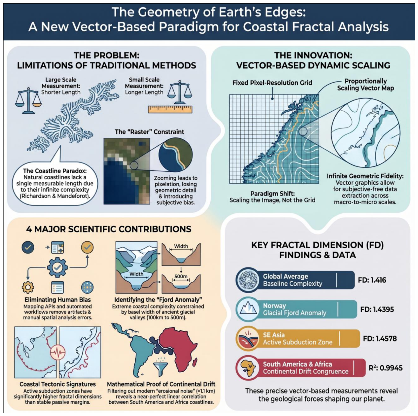
Figure 2.
Schematic workflow of the automated multi-scale coastal fractal analysis pipeline. (a) Cartographic Data Acquisition: Programmatic custom style injection into the Google Maps API and Gecko-based browser rendering to extract label-free land-water vectors and suppress WebKit-induced grid artifacts. (b) Digital Image Preprocessing: Grayscale conversion, CLAHE contrast optimization (adapthisteq), and Otsu binarization, followed by 8-connectivity connected-component spatial filtering and Canny edge detection to delineate a topologically closed, 1-pixel-wide marine coastline. (c) Dynamic Grid Scaling: Superposition of a constant pixel grid g over scalable vector geometries across zoom levels n, incorporating latitudinal scale-distortion correction: ϵ = gS0cosθ/2n. (d) Statistical Regression Diagnostics: Ordinary Least-Squares (OLS) linear regression in double-logarithmic space (logN(ϵ) vs. log(1/ϵ)) to mathematically extract the global bulk fractal dimension Db and scale-specific localized profiles Db(n).
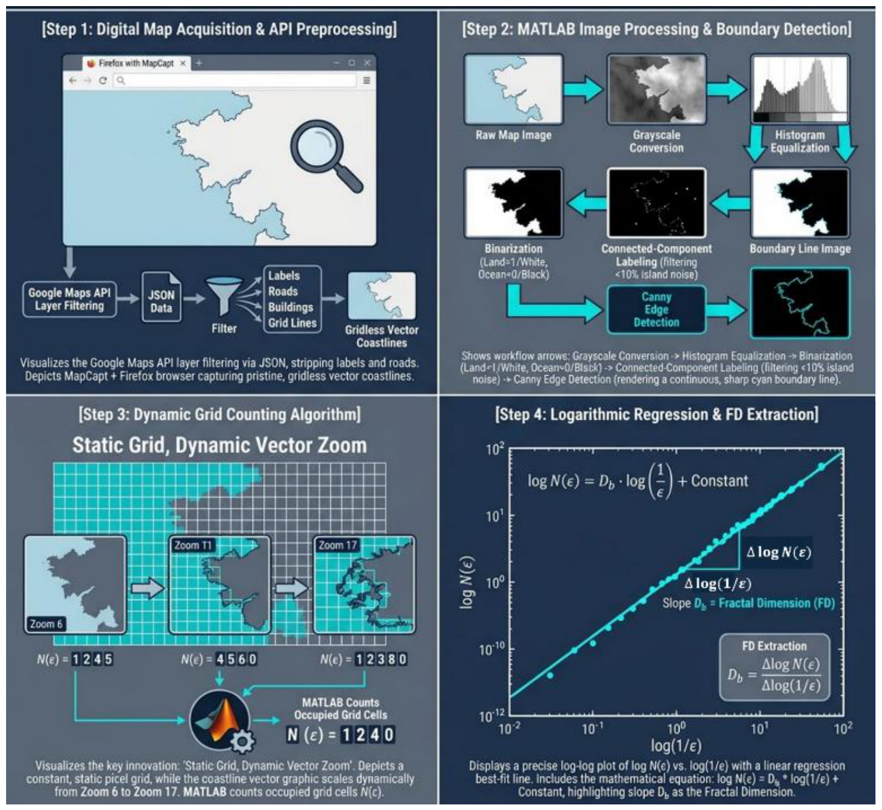
Figure 3.
Comparative Fractal Analysis of Coastal Complexity in Norway, Great Britain, and Taiwan. This figure presents a comparative multi-scale fractal analysis of coastal ruggedness across Norway, Great Britain, and Taiwan. Norway exhibits the highest complexity (Db = 1.4395), driven primarily by deeply indented glacial fjords, whereas Great Britain represents an intermediate benchmark (Db = 1.1858) for natural shorelines. Taiwan shows the lowest overall geometric complexity (Db = 1.0958) because of its smooth western alluvial plains, though anthropogenic structures synthetically alter its high-resolution signal.
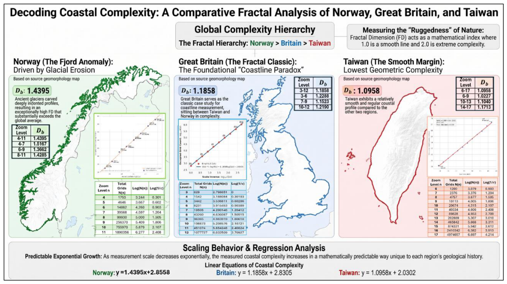
Figure 4.
Global Geographic Distribution of Coastal Fractal Complexity. This figure maps the global distribution of coastal complexity across 16 subdivisions. High-latitude North America exhibits the maximum global complexity (Db = 1.6909) due to deeply incised glacio-geomorphic fjord systems, while Northwest Europe (Db = 1.4416) and Southeast Asia (Db = 1.4578) show elevated complexities due to intense crustal deformation. Conversely, North Africa (Db = 1.0250) represents the lowest-ruggedness global baseline.
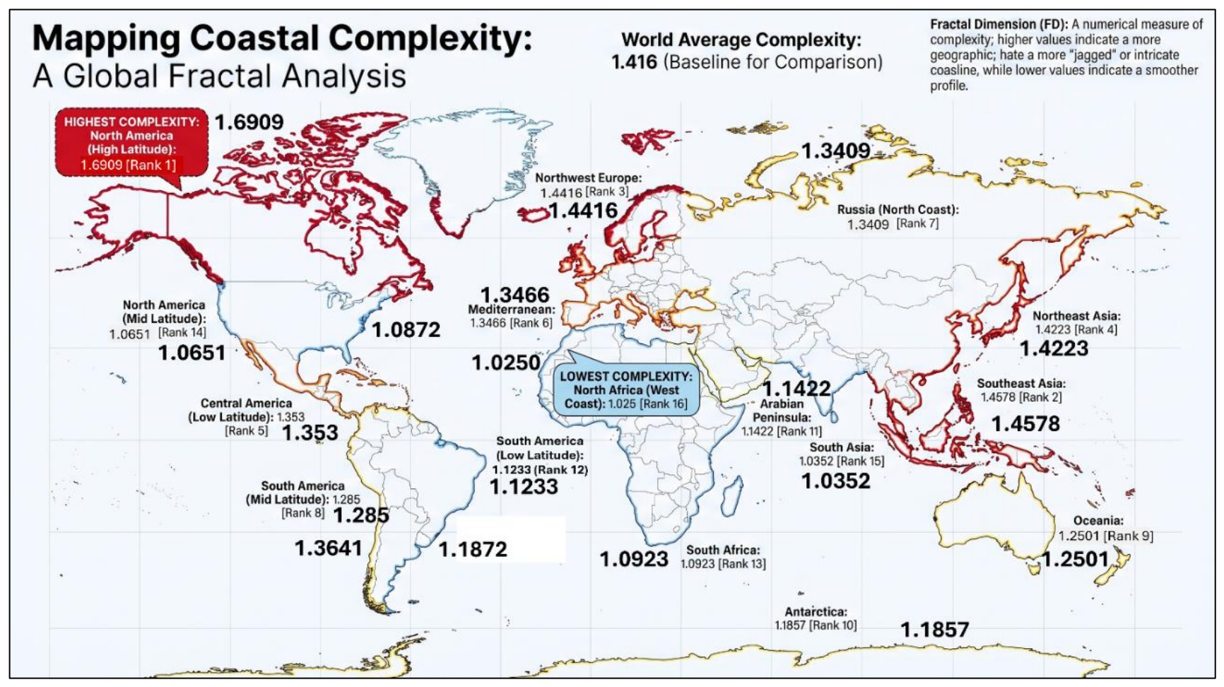
Figure 5.
Tectonic Fingerprints: Coastal Complexity Comparison Between Active Subduction Zones and Stable Margins. This schematic contrasts active convergent boundaries (Group 1, e.g., Southeast Asia, Northeast Asia) against stable passive and transform boundaries (Group 2, e.g., North Africa, South Asia), quantitatively demonstrating that tectonic compression and subduction systematically amplify fractal coastal complexity whereas strike-slip horizontal faulting and passive margin thermal subsidence structurally suppress it.
Disclaimer/Publisher’s Note: The statements, opinions and data contained in all publications are solely those of the individual author(s) and contributor(s) and not of MDPI and/or the editor(s). MDPI and/or the editor(s) disclaim responsibility for any injury to people or property resulting from any ideas, methods, instructions or products referred to in the content. |
© 2026 by the authors. Licensee MDPI, Basel, Switzerland. This article is an open access article distributed under the terms and conditions of the Creative Commons Attribution (CC BY) license (http://creativecommons.org/licenses/by/4.0/).
Copyright: This open access article is published under a Creative Commons CC BY 4.0 license, which permit the free download, distribution, and reuse, provided that the author and preprint are cited in any reuse.