

Submitted:
07 October 2026
Posted:
09 October 2026
You are already at the latest version
Abstract
Covariance augmentation expands small calibration sets for brain–computer interfaces (BCIs), but valid synthetic matrices need not preserve real-trial variation or improve cross-session decoding. We examined the relationship between covariance construction, distribution fidelity, and decoding performance. We compared real-only training with ambient noise followed by positive-definite projection, isotropic and class-dependent log-space noise, and same-class log-Euclidean interpolation on four motor-imagery electroencephalography (EEG) datasets with 3–60 channels. Using calibration draws paired across methods, we evaluated 83 subjects at 20 trials per class. Augmentation did not consistently improve balanced accuracy. Log-Euclidean interpolation changed accuracy by -0.25 to -0.01 percentage points (pp) and passed the additional Holm-corrected non-inferiority tests at a -5 pp group-mean margin. To determine whether near-neutral accuracy also reflected preserved variation, we compared synthetic samples with source trials excluded from calibration. Interpolation retained 62%–65% of the reference within-class scatter and had a larger energy distance than repeated real trials, despite remaining close to calibration class centers. Matched arithmetic interpolation lost more accuracy on two datasets; the methods differed little on the other two. We next tested the role of the classifier's covariance estimator. On BNCI2014_001 at 30 trials per class and augmentation ratio 3, changing fixed-ridge linear discriminant analysis (LDA) to automatic-shrinkage LDA shifted an isotropic-noise effect from -7.35 to +0.10 pp against the respective real-only baselines. Log-Euclidean interpolation and repeated real trials both lost approximately 1.9 pp under shrinkage. Finally, synthetic experiments with preserved labels and matched augmentation counts yielded similar gains from ambient and log-space noise under controlled covariance rotations. These results show that augmentation outcomes depend on both the generated distribution and classifier estimation. Positive definiteness provides valid covariance inputs; assessing fidelity and decoding utility requires independent distribution references and matched classifier comparisons.
Keywords:
electroencephalography
; EEG simulation
; brain–computer interface
; motor imagery
; covariance geometry
; Riemannian geometry
; data augmentation
; cross-session calibration
; MOABB
1. Introduction
A cross-session motor-imagery BCI uses EEG recorded in one session to decode trials from a later session. With a small labeled calibration set, augmentation increases the number of training samples. It also changes the class means and within-class variation on which the decoder is fitted. In covariance-based decoding, each trial is represented by a symmetric positive-definite (SPD) matrix that describes the covariance between EEG channels [1,6,7,8].
Positive definiteness constrains the construction of synthetic covariances, but several methods satisfy this requirement. Log-Euclidean methods apply noise or interpolation to the matrix logarithm and map the result back through the matrix exponential [3]. An alternative is to perturb covariance entries directly and project the result onto the SPD cone. Both constructions produce valid decoder inputs. The question is whether they preserve the variation in real trials and support decoding on a later session. This requires examining the generated distribution as well as accuracy.
To address this question, we compared real-only calibration with amplitude-matched ambient noise, isotropic log-space noise, class-dependent log-space noise, and same-class log-Euclidean interpolation. We used four public motor-imagery datasets, accessed through MOABB [2], spanning 3–60 EEG channels. Within each calibration draw, all methods received the same real trials. We averaged repeated draws within subject before statistical analysis, so comparisons reflected augmentation effects under the same calibration data.
We first evaluated cross-session accuracy across calibration budgets and measured how closely synthetic covariances remained to calibration class centers. These analyses raised two further questions: whether near-neutral accuracy and small class-center distances reflected preserved real-trial variation, and whether the large isotropic-noise loss at one budget depended on the classifier’s covariance estimator. We addressed them through independent source-trial references, matched interpolation and repeated-trial controls, and a comparison of covariance estimators. Finally, we tested the same augmentation methods under known covariance rotations in synthetic data. The Methods distinguish the original planned comparisons from the exploratory extensions; the supplement presents the literature-corpus analyses that motivated the study.
2. Materials and Methods
2.1. Study Design and Analysis History
We specified balanced accuracy at 20 real trials per class as the primary endpoint in the original protocol. The planned non-inferiority comparisons were G0 versus R0 on BNCI2014_001 and BNCI2014_004. G1, G2, Zhou2016, and the expansion of Stieger2021 from 10 to 62 subjects were added later and are reported as additional analyses. The original configuration is archived under docs/revision/archive_20261006/. We reaggregated accuracy and fidelity from all available subject records.
We specified the additional experiments in a protocol written on 6 October 2026 before those runs (scripts/revision/protocol.json). It fixed the calibration budgets, augmentation ratios, subjects, draw counts, classifiers, seeds, and distribution metrics. For these exploratory experiments, we generated new calibration draws paired across methods. We designed the second rotation experiment after examining the first synthetic results and report the two experiments separately.
2.2. Covariance Augmentation Methods
Let denote a real EEG trial for subject i, class c, and session s, with p channels and T samples. The trial covariance matrix is
where makes the covariance estimate strictly positive definite, including for short trials. G0, G1, and G2 operate in log-Euclidean coordinates [3,5]; the matrix exponential maps their symmetric outputs back to SPD matrices.
G0 adds symmetric isotropic Gaussian noise to each anchor’s matrix logarithm (Algorithm 1). G1 estimates a class-specific noise covariance using Ledoit–Wolf shrinkage [12]. G2 interpolates between two same-class anchors in log space (Algorithm 2). Comparing G1 and G2 with G0 tests the effects of class-dependent noise and interpolation.
For G2, the determinant is . It remains constant along the interpolation only if the two anchors have equal determinants. In log-covariance features, G2 is ordinary linear interpolation within a class and reduces the spread between anchors.
All three methods generate covariance features. We computed matrix logarithms and exponentials by eigendecomposition of symmetrized matrices. The primary settings were , , and across the MOABB datasets. Sensitivity analyses vary the noise scale and interpolation concentration; the classifier experiment also varies the augmentation ratio. Real EEG trials use the recorded source and target sessions, with no imposed covariance rotation.
| Algorithm 1:G0 – Log-Euclidean isotropic covariance jitter |
|
| Algorithm 2:G1 (empirical tangent Gaussian) and G2 (log-Euclidean geodesic mixup) |
|
2.3. Augmentation Baselines
The main non-transductive evaluation contains five conditions:
- R0 – Real-only calibration. Decoder trained on real calibration trials only.
- E0 – Amplitude-matched Euclidean perturbation. Symmetric Gaussian noise is added directly to covariance entries, followed by SPD projection through eigenvalue clipping at . A scalar root search sets the noise scale for each subject, budget, and resample. The target is G0’s median anchor-to-synthetic log-Euclidean distance, pooled across both classes under the same anchors and ratio. Synthetic samples retain their anchor labels. This control matches perturbation magnitude while allowing the distribution shape to differ.
- G0 – Log-Euclidean isotropic jitter (Algorithm 1).
- G1 – Empirical tangent Gaussian jitter (Algorithm 2, top branch).
- G2 – Log-Euclidean geodesic mixup (Algorithm 2, bottom branch).
A sixth condition, A0 – Riemannian alignment, aligns source covariances using the unlabeled target-session covariance mean. Because it has access to target statistics, we report it separately in the supplement and exclude it from both non-inferiority test families. E0, G0, G1, and G2 use only source data during fitting.
Figure 1 summarizes the study design.
2.4. Public EEG Datasets and Preprocessing
We used four public motor-imagery datasets through MOABB [2]: BNCI2014_001 [4], BNCI2014_004 [9], Zhou2016 [10], and Stieger2021 [11] (Table 2). They span 3–60 EEG channels. The BNCI datasets each contain 9 subjects and Zhou2016 contains 4. All 62 Stieger2021 subjects were processed. At the primary budget, 61 were eligible for LDA and CSP evaluation and 60 for MDM, based on source-trial availability and successful classifier evaluation.
After 8–30 Hz filtering and epoching, we estimated trial covariances with OAS shrinkage in pyriemann and added a ridge of . At each budget , each augmented condition generated 3 synthetic samples per real calibration trial (). We recorded the generator seeds for every draw in the calibration manifest.
Filtering and epoching used MOABB’s MotorImagery pipeline with the specified settings, without additional baseline correction or a separately specified Butterworth filter. Dataset-specific splits separated source calibration from later-session testing. For the additional Stieger2021 experiments, we used sessions 1 and 2 and retained the dataset’s 3 s minimum accepted trial length. Target labels were used only to evaluate predictions.
2.5. Classifiers
The primary classifier was a custom binary LDA using features, with weights on off-diagonal entries. Features were standardized using the training-set mean and standard deviation. The classifier estimated the pooled within-class covariance, added , and solved for the discriminant vector. The feature dimension was . A separate experiment compared this fixed-ridge estimator with automatic covariance shrinkage.
The secondary classifiers were affine-invariant minimum distance to class mean (MDM) [6] and covariance-CSP with log-variance features followed by LDA. Their results are in the supplement.
2.6. Covariance Fidelity Metrics
To characterize changes in the generated covariances, we computed six fidelity metrics for each augmentation method. We averaged values across draws and classes within each subject before group comparisons: (i) Log-Euclidean distance from the subject’s class-mean log-covariance, , where is the mean of the real calibration log-covariances; (ii) affine-invariant Riemannian distance , which measures class-center distance in a second covariance geometry; (iii) Pearson correlation between the eigenvalue spectra of the class-mean augmented covariance and the class-mean real covariance; (iv) trace ratio (total-power preservation; ideal value 1); (v) condition-number ratio , relative to the arithmetic mean of real calibration covariances; and (vi) anchor-to-synthetic perturbation distance , averaged in the fidelity files. E0 amplitude matching uses the median across synthetic trials from both classes. Its matching accuracy was checked from the logged target, achieved median, relative error, and success flag.
We regenerated synthetic covariances from the recorded seeds and calibration anchors for the fidelity analysis. Draw-level results are stored in results/protocol/*/subject_level_fidelity.csv and were averaged within subject before distance comparisons (Section 2.12).
2.7. Classifier Covariance-Estimation Experiment
To examine the role of classifier estimation in G0’s accuracy loss, we compared covariance estimators on BNCI2014_001 using all nine subjects, 20, 30, and 40 calibration trials per class, augmentation ratios of 1, 3, and 5, and 100 resamples per cell. R0, repeated real trials, G0, and G2 were evaluated with fixed-ridge LDA and automatic-shrinkage LDA (solver=lsqr, shrinkage=auto). Both classifiers standardized features using training data only. We measured accuracy on the target session and on source trials excluded from calibration. We also recorded the extreme eigenvalues and condition number of each classifier’s pooled feature covariance.
With 22 channels, each feature vector has 253 entries. At 30 real trials per class and ratio 3, augmentation gives 240 training rows; the unregularized pooled within-class covariance has rank at most 238. The original experiments used ratio 3 at every budget. By varying the budget and ratio independently, we tested whether the loss followed the number of training rows. Comparing the two covariance estimators then tested whether the loss depended on how these rows were used to fit the classifier.
2.8. Interpolation Controls and Independent Fidelity Reference
To distinguish interpolation geometry from the effect of adding dependent samples, we compared R0, repeated real trials, repeated log-Euclidean class means, arithmetic same-class interpolation, and G2 on all four datasets at 20 calibration trials per class and ratio 3. Arithmetic interpolation and G2 used the same anchors, partners, and coefficients . All four augmented conditions added the same number of samples and retained the anchor labels. Arithmetic interpolation produces SPD matrices because it is a convex combination of SPD inputs. The class-mean control repeats and has zero synthetic within-class variation.
We used source trials excluded from each calibration draw as an independent fidelity reference. This comparison tested whether synthetic samples preserved variation beyond the anchors used to generate them. In log-covariance features, we measured the synthetic-to-reference within-class scatter ratio, the distance between synthetic and reference class means, and the ratio of between-class mean separation. We also computed the class-averaged energy V statistic [13],
with diagonal pairs included in the within-set averages. Distances were divided by . This descriptive finite-sample statistic measures differences in distribution location and spread. Reference trials were excluded from generation and classifier fitting; target labels were used only for accuracy evaluation.
2.9. Controlled Synthetic Experiment
The synthetic experiment used 24 subjects, 8 channels, 128 samples per trial, 140 source and 220 target trials per class, 20 real calibration trials per class, ratio 3, and 30 resamples. Each subject had two class covariances with a shared random orthogonal basis. Their eigenvalues were linearly spaced from 1 to 1.45 and from 1.42 to 0.98. Gaussian trial samples received a lag-one contribution of 0.2, and covariance estimates received a diagonal ridge.
Target covariances were rotated by 0, 0.15, or 0.30 radians in a fixed plane of the subject’s orthogonal basis. Source data, calibration draws, augmentation seeds, and target sampling noise were paired across drift conditions. R0, E0, G0, G1, and G2 used the same implementations as the EEG experiments, with and . All augmented conditions retained the source labels and added the same number of samples. This design compared the methods’ responses to a known covariance rotation under a specified distribution.
The adjacent-eigenvector rotations produced little change in real-only accuracy. To test a rotation spanning a wider range of eigenvalues, we specified a separate exploratory follow-up in scripts/revision/rotation_stress_protocol.json before running it. This experiment rotates the first and last eigenvector directions, whose eigenvalues span the class spectra, by 0, 0.30, and 0.60 radians. All source data, target sampling noise, calibration draws, generator seeds, labels, counts, and classifier settings are paired with the first synthetic experiment. The original rotation results are retained alongside this follow-up.
2.10. Repeated Calibration Resampling
For each dataset, subject, and budget, we drew B class-balanced calibration sets from the source trials. We used for BNCI2014_001, BNCI2014_004, and Zhou2016, and for the 62-subject Stieger2021 cohort to limit computation at . All methods used the same real trials within a draw, holding calibration-set composition fixed in comparisons with R0. We generated new synthetic covariances for each draw using a deterministic SeedSequence derived from the protocol master seed. The target test set remained fixed across draws and methods. Each subject’s mean balanced accuracy over the B draws was the independent unit for group analysis.
2.11. Leakage Control
Target labels were used only to calculate balanced accuracy and macro-F1. Preprocessing settings were fixed before analysis and applied to both source and target sessions. Augmentation, parameter selection, and classifier fitting in the primary comparison used source data only. Trial indices and seeds were recorded in results/protocol/*/calibration_manifest.csv; docs/leakage_audit.md records which data each stage used. A0 alignment additionally uses unlabeled target covariances. It is therefore reported separately in the supplement as a target-informed comparator.
2.12. Statistical Analysis
We analyzed subject means over calibration draws. Descriptive 95% intervals were percentile bootstrap intervals from 5,000 subject resamples with seed 20261006. The two planned G0-versus-R0 tests on the BNCI datasets formed one Holm-corrected family. Additional comparisons at the primary budget formed a separate family of 16 tests: four methods across four datasets. For each comparison, a one-sided paired t test evaluated pp. Both unadjusted and Holm-adjusted p-values and the one-sided 95% lower bound were recorded. We based non-inferiority decisions on these one-sided tests; the two-sided bootstrap intervals describe uncertainty in the mean effects.
We chose a 5 pp margin for the group mean and repeated the 16-test family with margins of 3 and 7 pp in sensitivity analyses. To assess losses within each cohort, we also counted subjects with pp. A group can pass non-inferiority while some subjects lose more than this margin. Zhou2016 had four subjects, limiting the precision of its estimates.
A secondary model summarized effects across datasets: , where and . Covariance-distance comparisons were descriptive, with paired Wilcoxon tests. The classifier and interpolation experiments were reported using subject-level effects and descriptive intervals.
2.13. Software and Reproducibility
The original environment is specified in reproducibility/environment.yml. The additional experiments and result aggregation ran on Ubuntu; their Python and package versions are recorded in environment.json. The project retains source and input hashes, subject logs, covariance-cache manifests, calibration and reference indices, and draw-level results.
The calibration manifests allow reproduction of the original draws. The original planner derived seeds from Python’s process-dependent string hash; reproducing these draws across processes therefore requires the manifests in addition to the master seed. The additional experiments use stable SHA-256-derived seeds.
The EEG and synthetic experiments use the Python implementations in scripts/protocol/ and scripts/revision/. TensorEEG provides the accompanying R simulation package and covariance utilities (https://github.com/Yiming-S/TensorEEG). The reported Python experiments run independently of its R simulator. The controlled synthetic comparison uses the same five augmentation methods as the EEG experiments, with matched sample counts and unchanged class labels. Details of the earlier, superseded synthetic comparison are retained in the supplement.
2.14. Use of AI-Assisted Tools
OpenAI Codex assisted with study revision, implementation of experiment, result-aggregation and plotting code, and manuscript drafting and language editing. Numerical experiments were executed on Ubuntu using the archived protocols and code. Results, tables, and figures were checked against recorded outputs. The author is responsible for the final manuscript.
3. Results
3.1. Cross-Session Accuracy and Individual Losses
Augmentation did not consistently improve cross-session accuracy at the primary calibration budget. At 20 trials per class, the paired cohorts comprised 9 subjects from BNCI2014_001, 9 from BNCI2014_004, 4 from Zhou2016, and 61 from Stieger2021 (Table 3). Both planned G0 comparisons passed the pp non-inferiority test after Holm correction within the two-test family. In the additional 16-test family, all four methods passed on the two BNCI datasets and Stieger2021. On Zhou2016, G1 and G2 passed; E0 and G0 did not pass after Holm correction.
We then examined individual losses within the cohorts that passed the group test. Under E0, losses exceeded 5 pp in one of nine BNCI2014_001 subjects and five of 61 Stieger2021 subjects; the largest Stieger2021 loss was 10.15 pp. G0, G1, and G2 had no subject-mean losses exceeding 5 pp at this budget in those datasets. Thus, the group-level non-inferiority result coexisted with losses exceeding the margin for some subjects.
The effect of G0 also varied with calibration budget. It reduced accuracy by 7.24 pp at budget 30 on BNCI2014_001 (Figure 3). The augmentation ratio was three synthetic trials per real anchor at every budget. This budget-specific loss motivated the classifier comparison reported below. Stieger2021 contributed 62, 61, and 60 subjects at budgets 10, 20, and 30, respectively, so its cohort changed with budget.
The secondary dataset-random-intercept model included 83 paired subjects. The pooled G2 effect was pp (95% model-based interval ), with a between-dataset SD of 0.078 pp. This model summarizes the four observed datasets, while the dataset-specific estimates retain differences in transfer behavior.
3.2. Covariance Fidelity and Perturbation Matching
We next characterized the covariances generated by each method. The pooled fidelity analysis included 84 subjects. Each subject’s available budgets, resamples, and classes were averaged before pooling. Dimension-normalized log-Euclidean distances to the calibration log-class mean were 0.312 for E0, 0.226 for G0, 0.166 for G1, and 0.131 for G2. The corresponding affine-invariant distances were 0.354, 0.325, 0.216, and 0.180 (Table 4). G2 was closest to the calibration center in both geometries. To determine whether this proximity also reflected preserved real-trial variation, we compared it with an independent source reference in the interpolation experiment below.
G0 had a pooled trace ratio of 1.124 and a condition-number ratio of 0.416. E0 was near 1 on both ratios despite its larger class-center distances. G2’s trace ratio was 0.931. These metrics capture different properties of the generated covariances.
To verify that E0 and G0 had comparable perturbation magnitudes, we checked the recorded target and achieved median distances. All 15,945 E0 matching cells satisfied the configured 5% median-distance tolerance; the largest logged relative error was 3.01%. The fidelity file contains within-class mean anchor distances. Its E0/G0 ratio therefore describes a different quantity from the pooled median used for matching.
3.3. Effect of Covariance Estimation on Isotropic Jitter
To examine whether the G0 loss depended on classifier estimation, we repeated the comparison on BNCI2014_001 with independently seeded calibration draws. The loss was reproduced: at budget 30 and ratio 3, G0 reduced fixed-ridge LDA accuracy by 7.35 pp (95% subject bootstrap interval ). With automatic-shrinkage LDA, its effect against that classifier’s R0 baseline was pp (). On independent source trials, the corresponding effects were pp () and pp (). The loss under fixed-ridge estimation therefore extended to the source session as well as the later target session.
We next varied the augmentation ratio independently of the calibration budget. Increasing the ratio moved the loss to a smaller budget: at budget 20 and ratio 5, G0’s fixed-ridge effect was pp. This setting and budget 30 at ratio 3 both supplied 240 training rows for 253 features. At budget 30 and ratio 3, the median subject-mean condition number was 14,736 for fixed-ridge G0 and 14.2 for shrinkage G0. Fixed-ridge G2 had a larger condition number, 23,552, but an accuracy effect of pp. The condition number alone therefore did not account for the accuracy differences between methods.
The estimator comparison also changed the effects of G2 and repeated real trials. At budget 30 and ratio 3, their shrinkage-LDA effects were pp () and pp (), respectively; both were near zero with fixed-ridge LDA. Repeating trials leaves the empirical feature distribution unchanged but increases the number of training rows. The repeated-trial loss shows that the shrinkage classifier’s transfer accuracy can change when additional rows carry no new feature values. Figure 5 summarizes these comparisons; Supplementary Section gives the full numerical grid.
3.4. Matched Interpolation and Independent Distribution Reference
We next compared matched interpolation methods and controls to separate the effects of construction from sample repetition. The comparison included 9, 9, 4, and 61 subjects on BNCI2014_001, BNCI2014_004, Zhou2016, and Stieger2021, respectively. Stieger2021 subject 60 had 22 and 18 source trials in the two classes and was excluded because one class did not meet the 20-trial requirement. Repeating real trials changed fixed-ridge accuracy by less than 0.01 pp on every dataset. G2’s effects against R0 were , , , and pp in the same dataset order. Figure 6 shows subject and group effects, including the repeated-class-mean control, which has zero synthetic within-class variation.
Arithmetic interpolation reduced accuracy by 2.57 pp on BNCI2014_001 and 4.39 pp on Zhou2016. The paired G2-minus-arithmetic effects were pp () and pp (), respectively. On BNCI2014_004 and Stieger2021, they were pp () and pp (). G2 lost less accuracy than arithmetic interpolation on two datasets, although its group means remained slightly below R0 on all four. Supplementary Section shows the direct paired comparisons.
Near-neutral G2 accuracy was accompanied by a reduction in synthetic within-class variation. G2 retained 0.624, 0.621, 0.651, and 0.632 times the independent source within-class scatter across the four datasets. The ratios for repeated trials were 0.971, 0.968, 1.012, and 0.983. Arithmetic interpolation also reduced scatter, with ratios of 0.630, 0.646, 0.705, and 0.638. G2 had a larger energy distance to the independent reference than repeated trials on every dataset: 0.0155 versus 0.0133 on BNCI2014_001, 0.0321 versus 0.0262 on BNCI2014_004, 0.0246 versus 0.0218 on Zhou2016, and 0.0193 versus 0.0170 on Stieger2021. Repeated class means had zero scatter and much larger energy distances, even though their distance to the calibration log-class center was zero. These controls demonstrate why closeness to a calibration center and preservation of the independent reference distribution require separate comparisons.
3.5. Equal-Count, Label-Preserving Synthetic Comparison
Finally, we evaluated the same methods under controlled covariance rotations, with matched augmentation counts and preserved labels. At zero rotation, mean R0 accuracy across the 24 synthetic subjects was 79.05%. E0 and G0 raised it to 97.35% and 97.58%, with paired gains of pp () and pp (). G1 gained 8.31 pp and G2 gained 0.45 pp. This ordering persisted at rotations of 0.15 and 0.30 radians (Figure 8a,c). R0 stayed between 79.02% and 79.05%, showing little response to these adjacent-eigenvector rotations. E0 and G0 produced similar gains despite using different covariance constructions.
In the endpoint-eigenvector follow-up, R0 fell from 79.05% at zero rotation to 76.59% at 0.30 radians and 69.21% at 0.60 radians. At 0.60 radians, E0 and G0 reached 88.61% and 88.70%, with gains of pp () and pp (). G1 gained 6.58 pp and G2 gained 0.25 pp. All 3,600 zero-rotation records matched the first experiment. The larger rotation reduced baseline accuracy, while the method ordering and the similar E0 and G0 gains persisted. Figure 8 compares both designs; Supplementary Section gives their numerical results.
4. Discussion
We examined covariance augmentation through two complementary outcomes: decoding on a later session and preservation of real-trial variation. Across the four EEG datasets, augmentation did not provide consistent accuracy gains. G2 combined near-neutral fixed-ridge accuracy with a contracted synthetic distribution, while the large G0 loss changed with the classifier’s covariance estimator. These findings link the performance of an augmentation method to both its generated samples and the estimator fitted to them.
4.1. Effects of the Classifier’s Covariance Estimator
The classifier comparison showed that G0’s accuracy loss depended on covariance estimation. At budget 30 and ratio 3, its effect changed from pp with fixed-ridge LDA to pp with automatic shrinkage. The fixed-ridge loss also occurred on independent source trials, so cross-session drift was not required for it to appear. At budget 20 and ratio 5, the loss occurred with the same 240 training rows and 253 features. The dependence on estimator and training-set size supports examining classifier estimation when interpreting augmentation losses.
The conditioning results qualify this interpretation. G2 and repeated trials can have larger pooled covariance condition numbers than G0 while preserving fixed-ridge accuracy. Thus, the condition number alone does not explain the method ordering. The observed estimator dependence concerns nine subjects and log-covariance features; extending it to other representations requires direct evaluation.
Automatic shrinkage also changed G2’s effect. At budget 30 and ratio 3, G2 lost 1.92 pp, close to the 1.95 pp loss from repeated trials. Exact repetition leaves the empirical feature distribution unchanged but supplies more rows to covariance estimation. This control shows why augmentation comparisons need to account for the classifier’s response to dependent samples as well as the construction of synthetic covariances.
4.2. Class-Center Distance and Real-Trial Variation
G2’s small class-center distance has a direct explanation in its construction. The calibration centers were estimated from the same anchors used to generate synthetic samples. In log-covariance features, G2 linearly interpolates between same-class vectors. This construction pulls samples toward the class center and reduces their spread. Repeating class means provides the limiting example, with zero class-center distance and zero within-class scatter. Measuring variation against independent real trials is therefore necessary to interpret proximity to a calibration center.
The independent-reference comparison showed that G2 retained 62%–65% of real within-class scatter and had a larger energy distance than repeated trials on every dataset. Arithmetic interpolation also reduced scatter. G2’s small class-center distance and near-neutral fixed-ridge accuracy therefore coexisted with a contracted synthetic distribution. Accuracy alone would not reveal this change in within-class variation.
Matching anchors, partners, and interpolation weights allowed us to compare the two constructions directly. G2 lost less accuracy than arithmetic interpolation on BNCI2014_001 and Zhou2016, but the difference was small on BNCI2014_004 and Stieger2021. G2 remained slightly below the real-only group mean on all four. The choice of interpolation geometry affected accuracy in two cohorts. The independent-reference metrics provide a separate assessment of how much real-trial variation the synthetic samples retained.
4.3. Augmentation Under Controlled Covariance Rotations
The synthetic experiments identified conditions in which augmentation improved accuracy. E0 and G0 produced similar large gains, while G2’s gain was small. Adjacent-eigenvector rotations barely changed baseline accuracy. The endpoint rotation reduced it by 9.84 pp at 0.60 radians, yet E0 and G0 retained similar gains. Thus, the benefit of augmentation persisted when the rotation measurably reduced baseline accuracy. Because ambient and log-space noise performed similarly, this benefit cannot be attributed uniquely to the log-Euclidean construction.
4.4. Evaluation and Scope
These results define the information needed to interpret an augmentation comparison: the calibration budget, synthetic-to-real ratio, covariance construction, classifier estimator, and access to target data. Repeated trials test the effect of adding dependent rows, while matched arithmetic and log-space interpolation compare covariance construction. Source trials excluded from calibration provide a distribution reference that is independent of generation and fitting and does not require target labels.
Our EEG experiments evaluated offline session transfer in public motor-imagery datasets. Each BNCI cohort had nine subjects and Zhou2016 had four. Stieger2021 provided broader subject coverage but used 15 calibration resamples per cell. Pooled fidelity weighted subjects equally, giving Stieger2021 most of the weight; the per-dataset summaries indicate whether patterns were shared across cohorts. The planned G0 tests and exploratory comparisons were analyzed separately. The 5 pp non-inferiority margin applied to the group mean. Individual losses exceeding that margin demonstrate the need to retain subject-level results alongside group decisions.
The synthetic experiments allowed us to compare the same methods under a known covariance rotation and a specified distribution. The scope of this study is covariance-feature augmentation for offline motor-imagery decoding. Waveform generation, trained generative models, and prospective online BCI require evaluation under their respective inputs and operating conditions.
5. Conclusions
We compared covariance augmentation across four cross-session motor-imagery datasets and found that its effects varied with construction, calibration budget, and classifier. Augmentation did not consistently improve decoding accuracy. The large G0 loss under fixed-ridge LDA was reproduced with independent calibration draws, while its effect was near zero under automatic shrinkage. G2 remained near neutral with fixed-ridge LDA, but contracted synthetic variation and lost accuracy under shrinkage. Ambient and log-space noise yielded similar gains in the controlled synthetic experiments.
These comparisons establish distinct roles for covariance validity, distribution fidelity, and decoding utility. Positive definiteness ensures valid decoder inputs. Independent-reference scatter and distance assess preservation of real-trial variation, while subject-level accuracy effects and losses assess utility. Matched interpolation, repeated-trial controls, and classifier comparisons are needed to interpret how covariance construction and estimation contribute to the observed performance.
Supplementary Materials
The following supporting information can be downloaded at the website of this paper posted on Preprints.org. The supplement provides corpus methods and sensitivity analyses, secondary classifiers, target-informed alignment, augmentation parameter sensitivity, perturbation matching, and complete tables for the classifier and interpolation experiments. It also documents the superseded synthetic comparison.
Author Contributions
Conceptualization, Y.S.; methodology, Y.S.; software, Y.S.; validation, Y.S.; formal analysis, Y.S.; investigation, Y.S.; data curation, Y.S.; writing—original draft preparation, Y.S.; writing—review and editing, Y.S.; visualization, Y.S. The author approved the final manuscript.
Funding
This research received no external funding.
Institutional Review Board Statement
Ethical review and approval were not required for this secondary analysis because only publicly available, anonymized EEG datasets were analysed. The original dataset publications should be consulted for their ethics approvals.
Informed Consent Statement
Not applicable to the present secondary analysis of public anonymized datasets.
Data Availability Statement
Public EEG data are accessed through MOABB [2]. The project contains the R package, Python experiment scripts, calibration manifests and draw-level outputs, the protocols, code and input hashes, and additional experiment outputs under results/revision_20261006/. The TensorEEG source repository is maintained at https://github.com/Yiming-S/TensorEEG. The accompanying supplementary archive contains the experiment and analysis code, protocols, calibration manifests, draw-level results, summaries, recorded environments, and the OpenAlex corpus snapshot. Raw EEG recordings are obtained from the original public datasets through MOABB and are not redistributed in the archive.
Conflicts of Interest
The author declares no conflicts of interest.
References
- Lotte, F.; et al. , A review of classification algorithms for EEG-based brain–computer interfaces: A 10 year update. J. Neural Eng. 2018, vol. 15(no. 3), 031005. [Google Scholar] [CrossRef] [PubMed]
- Jayaram, V.; Barachant, A. MOABB: Trustworthy algorithm benchmarking for BCIs. J. Neural Eng. 2018, vol. 15(no. 6), 066011. [Google Scholar] [CrossRef] [PubMed]
- Arsigny, V.; Fillard, P.; Pennec, X.; Ayache, N. Geometric means in a novel vector space structure on symmetric positive-definite matrices. SIAM J. Matrix Anal. Appl. 2007, vol. 29(no. 1), 328–347. [Google Scholar] [CrossRef]
- Tangermann, M.; et al. , Review of the BCI Competition IV. Front. Neurosci. 2012, vol. 6, 55. [Google Scholar] [CrossRef] [PubMed]
- Pennec, X.; Fillard, P.; Ayache, N. A Riemannian framework for tensor computing. Int. J. Comput. Vis. 2006, vol. 66(no. 1), 41–66. [Google Scholar] [CrossRef]
- Barachant, A.; Bonnet, S.; Congedo, M.; Jutten, C. Multiclass brain-computer interface classification by Riemannian geometry. IEEE Trans. Biomed. Eng. 2012, vol. 59(no. 4), 920–928. [Google Scholar] [CrossRef] [PubMed]
- Blankertz, B.; et al. Optimizing spatial filters for robust EEG single-trial analysis. IEEE Signal Process. Mag. 2008, vol. 25(no. 1), 41–56. [Google Scholar] [CrossRef]
- Koles, Z. J.; Lazar, M. S.; Zhou, S. Z. Spatial patterns underlying population differences in the background EEG. Brain Topogr. 1990, vol. 2(no. 4), 275–284. [Google Scholar] [CrossRef] [PubMed]
- Leeb, R.; Lee, F.; Keinrath, C.; Scherer, R.; Bischof, H.; Pfurtscheller, G. Brain–computer communication: Motivation, aim, and impact of exploring a virtual apartment. IEEE Trans. Neural Syst. Rehabil. Eng. 2007, vol. 15(no. 4), 473–482. [Google Scholar] [CrossRef] [PubMed]
- Zhou, B.; Wu, X.; Lv, Z.; Zhang, L.; Guo, X. A fully automated trial selection method for optimization of motor imagery based brain-computer interface. PLoS ONE 2016, vol. 11(no. 9), e0162657. [Google Scholar] [CrossRef] [PubMed]
- Stieger, J. R.; Engel, S. A.; He, B. Continuous sensorimotor rhythm based brain computer interface learning in a large population. Sci. Data 2021, vol. 8, 98. [Google Scholar] [CrossRef] [PubMed]
- Ledoit, O.; Wolf, M. A well-conditioned estimator for large-dimensional covariance matrices. J. Multivar. Anal. 2004, vol. 88(no. 2), 365–411. [Google Scholar] [CrossRef]
- Székely, G. J.; Rizzo, M. L. Energy statistics: A class of statistics based on distances. J. Stat. Plan. Inference 2013, vol. 143(no. 8), 1249–1272. [Google Scholar] [CrossRef]
- Wang, L.; et al. MiniLM: Deep self-attention distillation for task-agnostic compression of pre-trained transformers. arXiv 2020, arXiv:2002.10957. [Google Scholar]
- McInnes, L.; Healy, J.; Melville, J. UMAP: Uniform manifold approximation and projection for dimension reduction. arXiv 2018, arXiv:1802.03426. [Google Scholar]
- Campello, R. J. G. B.; Moulavi, D.; Sander, J. Density-based clustering based on hierarchical density estimates. Proc. PAKDD 2013, 160–172. [Google Scholar] [CrossRef]
- Grootendorst, M. BERTopic: Neural topic modelling with a class-based TF-IDF procedure. arXiv 2022, arXiv:2203.05794. [Google Scholar]
- Killick, R.; Fearnhead, P.; Eckley, I. A. Optimal detection of changepoints with a linear computational cost. J. Amer. Stat. Assoc. 2012, vol. 107(no. 500), 1590–1598. [Google Scholar] [CrossRef]
- Benjamini, Y.; Hochberg, Y. Controlling the false discovery rate: A practical and powerful approach to multiple testing. J. R. Stat. Soc. Ser. B 1995, vol. 57(no. 1), 289–300. [Google Scholar] [CrossRef]
- Reimers, N.; Gurevych, I. Sentence-BERT: Sentence embeddings using Siamese BERT-networks. Proc. Conf. Empir. Methods Nat. Lang. Process. (EMNLP), Hong Kong, China, 2019; pp. 3982–3992. [Google Scholar] [CrossRef]
- Devlin, J.; Chang, M.-W.; Lee, K.; Toutanova, K. BERT: Pre-training of deep bidirectional transformers for language understanding. Proc. Conf. North Am. Chapter Assoc. Comput. Linguist. (NAACL-HLT), Minneapolis, MN, USA, 2019; pp. 4171–4186. [Google Scholar] [CrossRef]
- Cohan, A.; et al. SPECTER: Document-level representation learning using citation-informed transformers. Proc. Conf. Assoc. Comput. Linguist. (ACL) 2020, 2270–2282. [Google Scholar] [CrossRef]
- Lee, J.; et al. , BioBERT: A pre-trained biomedical language representation model for biomedical text mining. Bioinformatics 2020, vol. 36(no. 4), 1234–1240. [Google Scholar] [CrossRef] [PubMed]
- Beltagy, I.; Lo, K.; Cohan, A. SciBERT: A pretrained language model for scientific text. Proc. Conf. Empir. Methods Nat. Lang. Process. (EMNLP), Hong Kong, China, 2019; pp. 3615–3620. [Google Scholar] [CrossRef]
Figure 1.
Paired study design. a, Source trials provide balanced calibration draws and an excluded-trial reference; the later session supplies the fixed target set. b, R0 uses real trials only; E0/G0/G1/G2 augment the same anchors, and classifiers are fitted on source data. c, Target accuracy and covariance fidelity are separate outcomes. Fidelity is measured against calibration class centers and independent source trials, including variation and distributional distance. Repeated draws are averaged within subject before paired contrasts.
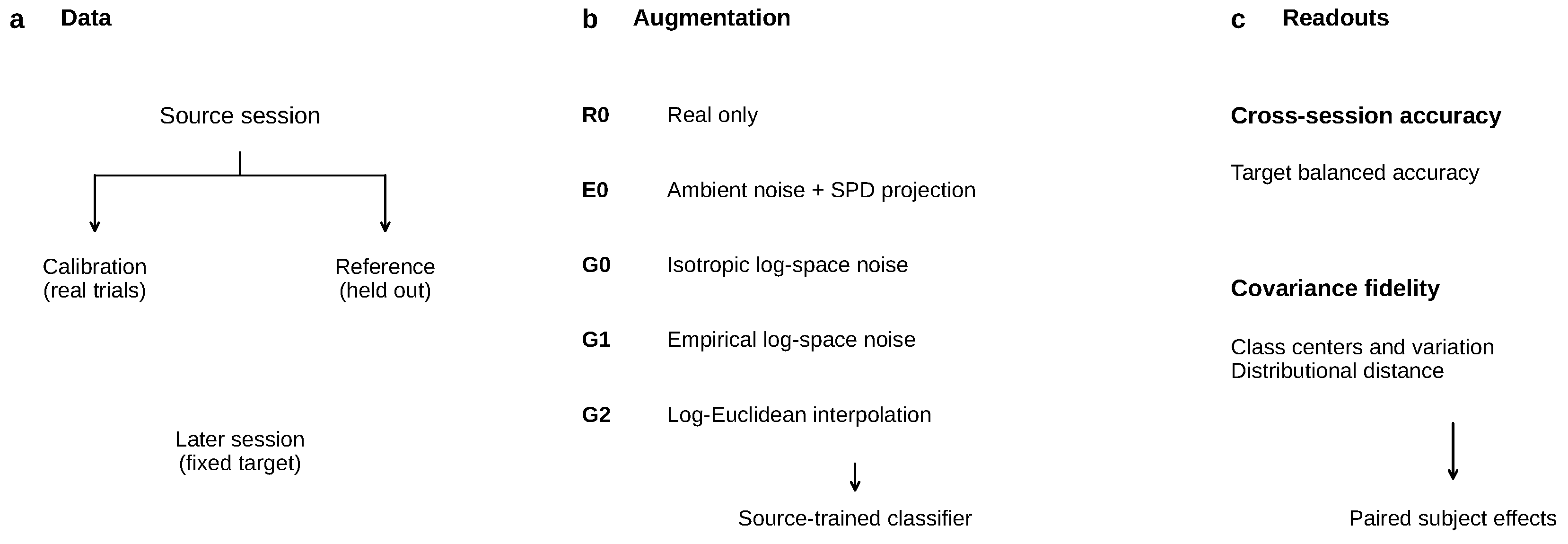
Figure 2.
Subject-level paired differences at budget 20. Points are means over calibration resamples; squares and whiskers are the group mean and 95% subject bootstrap interval. The dashed line marks the analysis-defined pp group-mean margin.
Figure 2.
Subject-level paired differences at budget 20. Points are means over calibration resamples; squares and whiskers are the group mean and 95% subject bootstrap interval. The dashed line marks the analysis-defined pp group-mean margin.
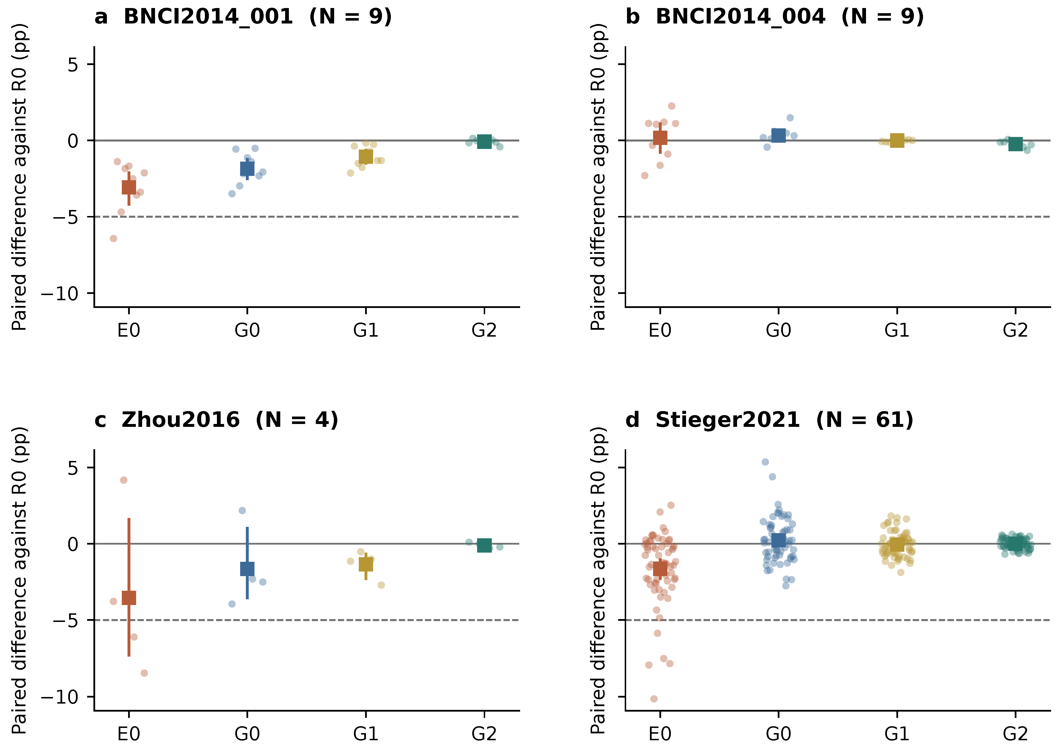
Figure 3.
Calibration curves. Lines are mean balanced accuracy across eligible subjects; shading gives descriptive 95% subject bootstrap intervals. The Stieger2021 cohort varies with budget (62, 61, and 60 subjects at budgets 10, 20, and 30).
Figure 3.
Calibration curves. Lines are mean balanced accuracy across eligible subjects; shading gives descriptive 95% subject bootstrap intervals. The Stieger2021 cohort varies with budget (62, 61, and 60 subjects at budgets 10, 20, and 30).
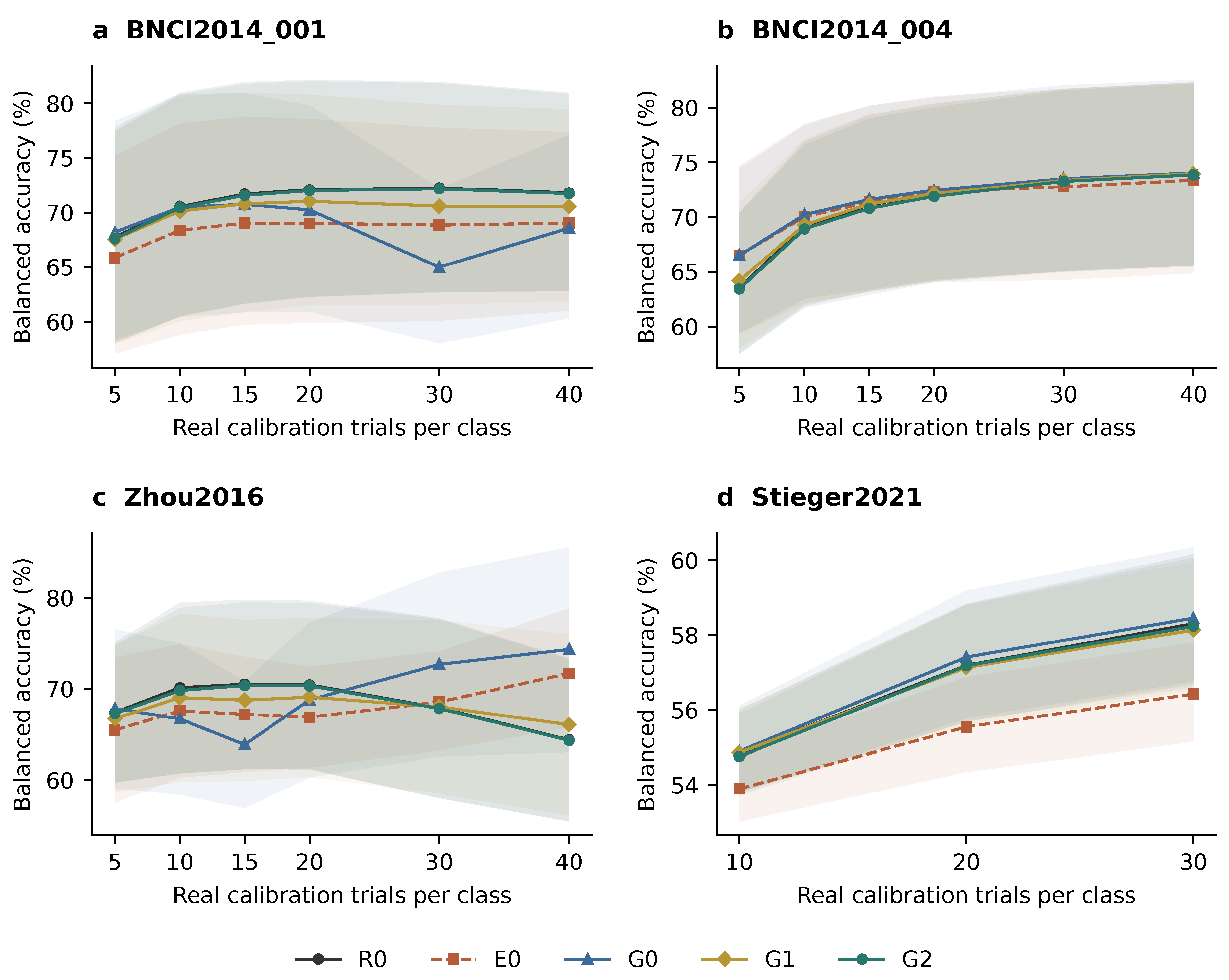
Figure 4.
Pooled fidelity across 84 subject-level means. Small points represent subjects; squares and whiskers show means and 95% subject bootstrap intervals. Distances are normalized by . Dashed lines mark a ratio of 1. Class-center distance, trace ratio, and conditioning describe distinct effects.
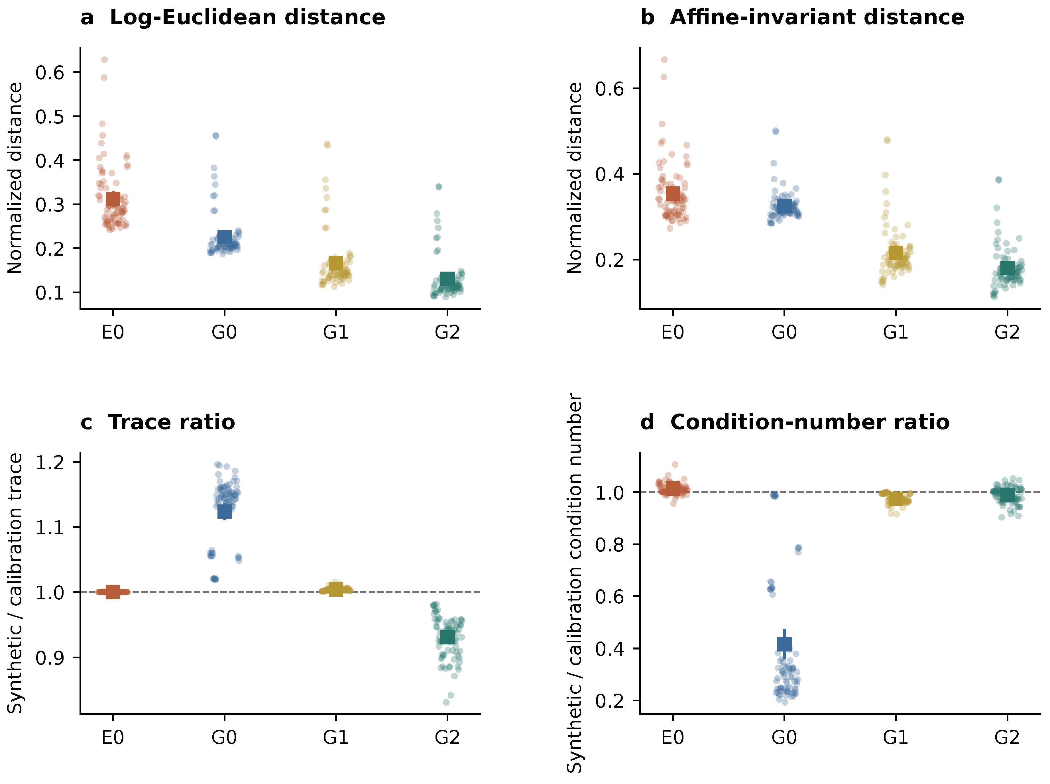
Figure 5.
Classifier-dependent augmentation effects on BNCI2014_001. (a,b) G0 target-accuracy differences against each classifier’s own R0 baseline across budgets and ratios. (c) Repeated real anchors, G0, and G2 at budget 30 and ratio 3. (d) G0 effects on independent source trials and the later target session at the same setting. Points and whiskers are subject means and descriptive 95% subject bootstrap intervals (, 100 resamples per cell). The dashed pp line marks the group-mean non-inferiority margin.
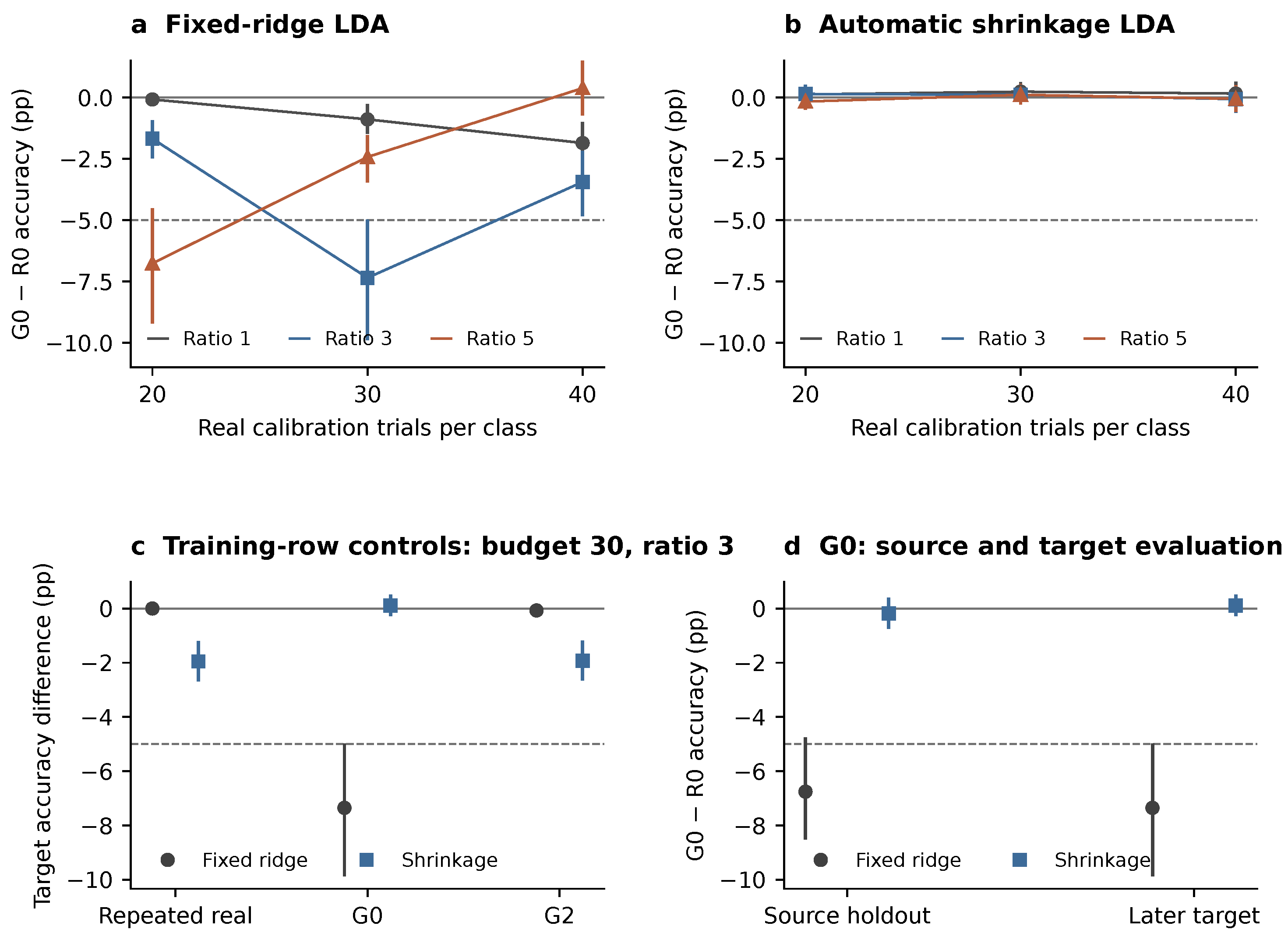
Figure 6.
Target accuracy of the four matched augmentation controls at budget 20 and ratio 3. Small points are paired subject-mean differences against R0; squares and whiskers are group means and 95% subject bootstrap intervals. Augmentation counts and labels are matched. Dataset panels use separate horizontal scales to show the range of subject effects.
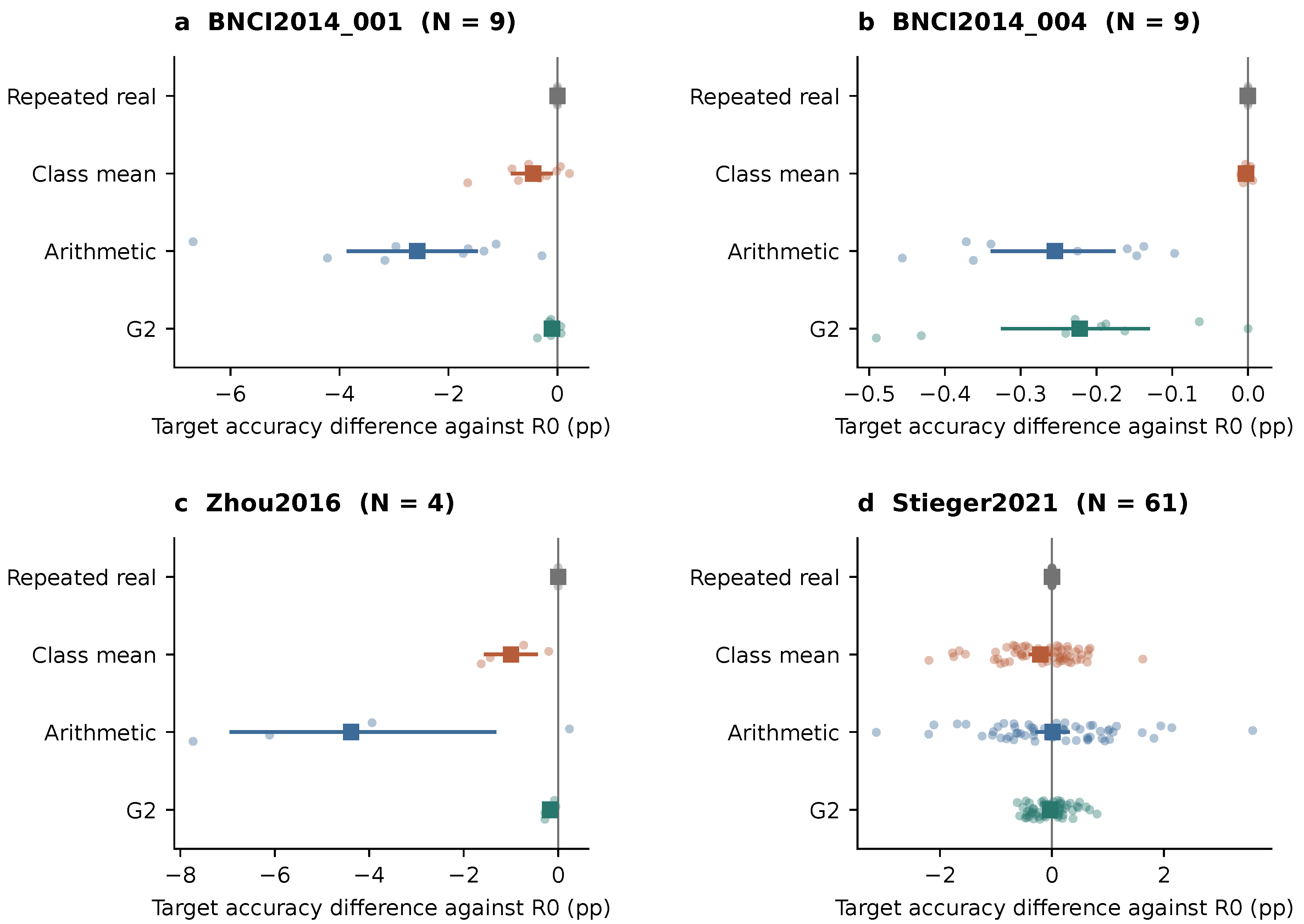
Figure 7.
Fidelity against independent source trials at budget 20 and ratio 3. (a) Within-class scatter ratio. (b) Class-averaged energy distance. (c) Distance between synthetic and reference class means. (d) Between-class separation ratio. Points and whiskers give means and 95% subject bootstrap intervals; dataset counts are 9, 9, 4, and 61. Distances are normalized by ; dashed lines mark ratio 1. Reference trials are excluded from calibration, generation, and classifier fitting.
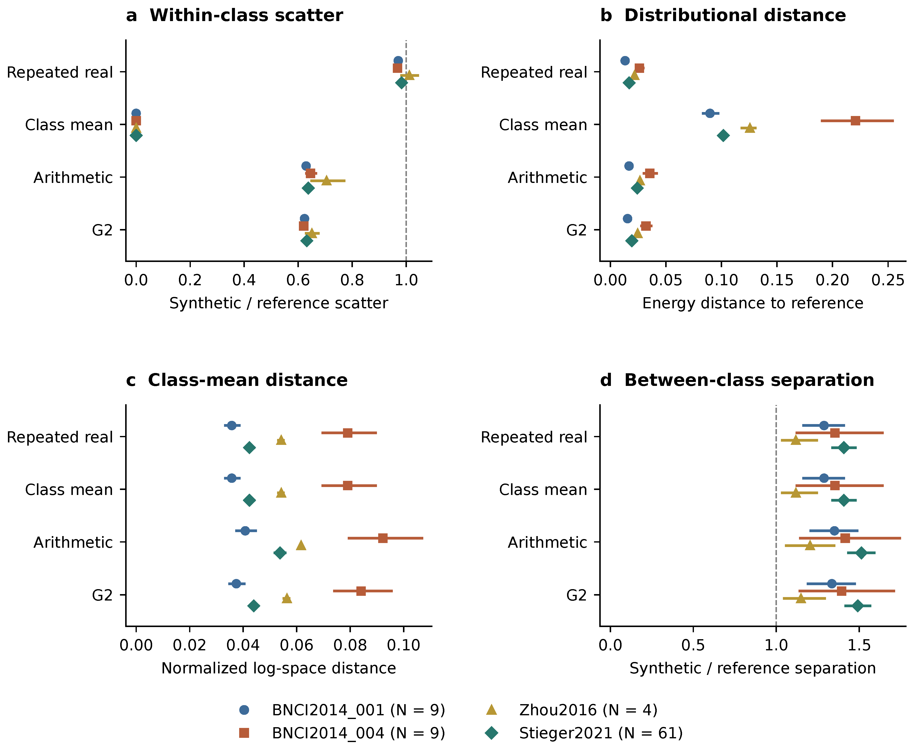
Figure 8.
Equal-count, label-preserving synthetic comparison. (a,c) Original adjacent-eigenvector rotations. (b,d) Separately specified exploratory endpoint-eigenvector follow-up. The top row shows absolute target balanced accuracy; the bottom row shows paired gains against R0. Whiskers are 95% subject bootstrap intervals (, 30 resamples per condition). Panels share vertical scales within each row. Source data, sampling noise, calibration draws, and augmentation seeds are paired across designs; the two designs have identical zero-rotation results.
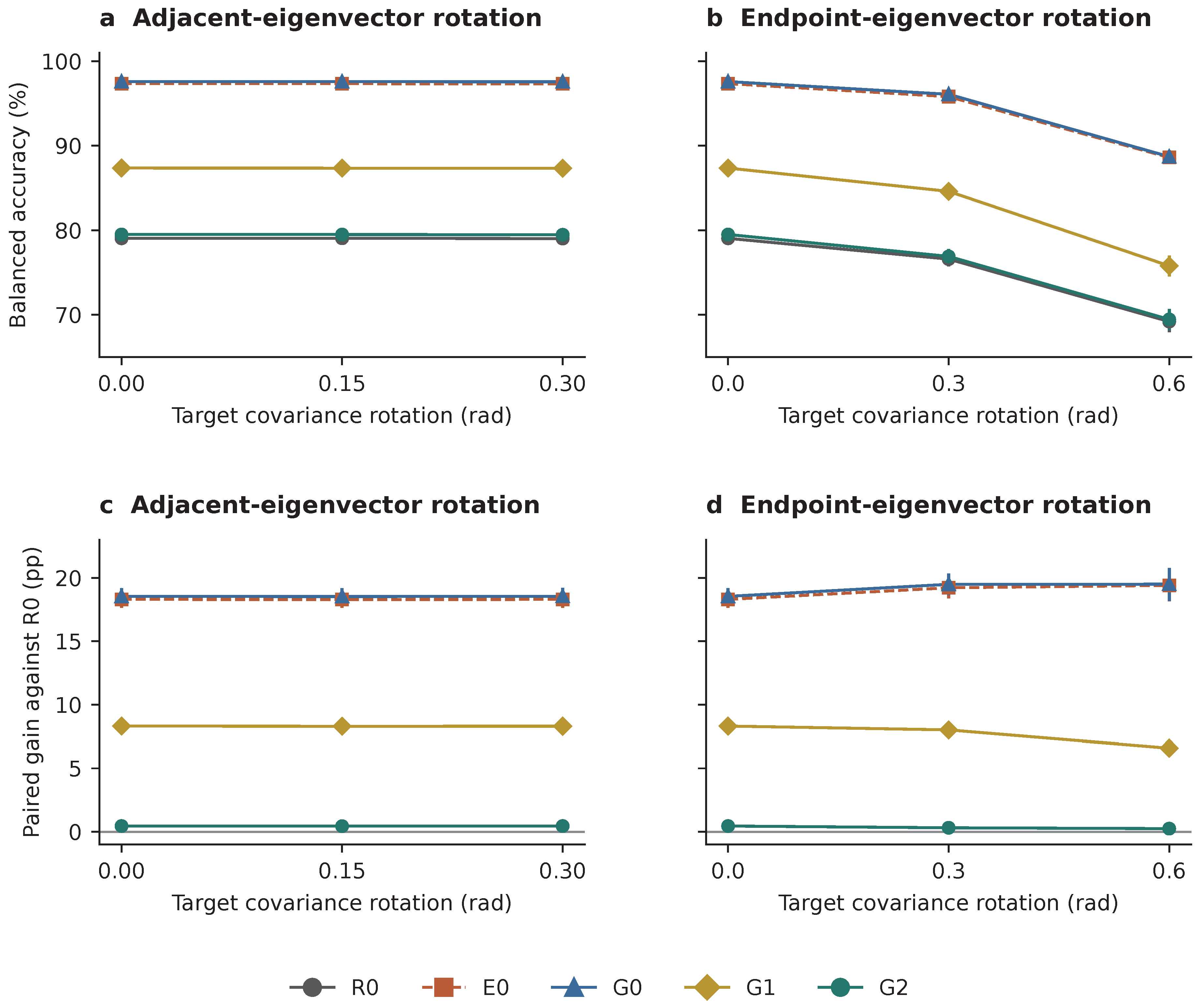

Table 1.
All augmentation conditions provide SPD decoder inputs. Construction and access to target-session statistics distinguish the methods.
Table 1.
All augmentation conditions provide SPD decoder inputs. Construction and access to target-session statistics distinguish the methods.
| Code | Construction | Target statistics |
|---|---|---|
| R0 | Real covariances | None |
| E0 | Ambient noise, then SPD projection | None |
| G0 | Isotropic log-space noise, then exponential | None |
| G1 | Class-dependent log-space noise, then exponential | None |
| G2 | Same-class log-Euclidean interpolation | None |
| A0 | Covariance alignment | Unlabeled target mean |
Table 2.
Public EEG datasets and cross-session protocol. All four datasets are accessed through MOABB [2] under the MI paradigm ( Hz, Hz, epoch 0.5–2.5 s post-cue). The evaluated budgets are shown separately for each dataset; the primary endpoint is evaluated at . Calibration sets are drawn by repeated balanced resampling (Section 2.10); within a resample the same real trial indices are shared across methods. Trial counts below are per subject per session per class.
| BNCI2014_001 | BNCI2014_004 | Zhou2016 | Stieger2021 | |
|---|---|---|---|---|
| Subjects at budget 20 (LDA) | 9 | 9 | 4 | 61 |
| Sessions available / subject | 2 | 5 | 3 | 7–11 |
| Channels | 22 | 3 (C3, Cz, C4) | 14 | 60 |
| Sampling rate (Hz) | 250 | 250 | 250 | 1000 |
| Native classes | 4 (LH, RH, feet, tongue) | 2 (LH, RH) | 3 (LH, RH, feet) | 4 (LH, RH, both, rest) |
| Classes used | LH vs. RH | LH vs. RH | LH vs. RH | LH vs. RH |
| Trials / session / class | ≈72 | ≈60–80 | ≈50–100 | ≈50–75 |
| Calibration / test split | Session 1 → 2 | Sessions 1–3 → 4–5 | Session 1 → 3 | Session 1 → 2 |
| Calibration budgets evaluated | ||||
| Resamples per cell (B) | 100 | 100 | 100 | 15 |
| Role in inference | Primary NI | Primary NI | Failure boundary | Additional high-channel |
Table 3.
Mean paired balanced-accuracy differences against R0 at 20 trials per class, in percentage points, with 95% subject bootstrap intervals. Intervals are descriptive; non-inferiority decisions use the one-sided paired t test and the stated Holm family.
Table 3.
Mean paired balanced-accuracy differences against R0 at 20 trials per class, in percentage points, with 95% subject bootstrap intervals. Intervals are descriptive; non-inferiority decisions use the one-sided paired t test and the stated Holm family.
| Dataset | N | E0 | G0 | G1 | G2 |
|---|---|---|---|---|---|
| BNCI2014_001 | 9 | [-4.18,-2.12] | [-2.51,-1.24] | [-1.51,-0.63] | [-0.18,+0.01] |
| BNCI2014_004 | 9 | [-0.79,+1.10] | [+0.03,+0.68] | [-0.05,+0.04] | [-0.38,-0.12] |
| Zhou2016 | 4 | [-7.29,+1.60] | [-3.54,+1.01] | [-2.29,-0.68] | [-0.26,+0.05] |
| Stieger2021 | 61 | [-2.28,-1.06] | [-0.13,+0.60] | [-0.26,+0.15] | [-0.09,+0.08] |
Table 4.
Dimension-normalized covariance fidelity, pooled across 84 subject-level means. Values are mean ± between-subject SD; distances are divided by .
Table 4.
Dimension-normalized covariance fidelity, pooled across 84 subject-level means. Values are mean ± between-subject SD; distances are divided by .
| Metric | E0 | G0 | G1 | G2 |
|---|---|---|---|---|
| Log-Euclidean distance | ||||
| Affine-invariant distance | ||||
| Anchor distance (mean) |
Table 5.
Raw fidelity metrics pooled across 84 subject-level means. Class-center references are derived from the calibration anchors. The ideal trace and condition-number ratios are 1.
Table 5.
Raw fidelity metrics pooled across 84 subject-level means. Class-center references are derived from the calibration anchors. The ideal trace and condition-number ratios are 1.
| Metric | E0 | G0 | G1 | G2 |
|---|---|---|---|---|
| Log-Euclidean distance | ||||
| Affine-invariant distance | ||||
| Eigenvalue correlation | ||||
| Trace ratio | ||||
| Condition-number ratio | ||||
| Anchor distance (mean) |
Disclaimer/Publisher’s Note: The statements, opinions and data contained in all publications are solely those of the individual author(s) and contributor(s) and not of MDPI and/or the editor(s). MDPI and/or the editor(s) disclaim responsibility for any injury to people or property resulting from any ideas, methods, instructions or products referred to in the content. |
© 2026 by the authors. Licensee MDPI, Basel, Switzerland. This article is an open access article distributed under the terms and conditions of the Creative Commons Attribution (CC BY) license (http://creativecommons.org/licenses/by/4.0/).
Copyright: This open access article is published under a Creative Commons CC BY 4.0 license, which permit the free download, distribution, and reuse, provided that the author and preprint are cited in any reuse.