

Submitted:
06 October 2026
Posted:
09 October 2026
You are already at the latest version
Abstract
Rain gauge network design requires both information retention and observations that support consequential decisions. We connect joint entropy, total correlation and value of information (VOI) using rainfall-network results for the Rio das Velhas basin, Brazil, and an analytical decision model. The study considers 39 observed gauges, including 28 within the basin, and 101 interpolated candidate locations. Configurations of 10, 12 and 15 gauges retain 85.6%, 88.2% and 90.8% of the reference joint entropy of 7.29 bits; the 15-gauge configuration retains more than 90% with 46.4% fewer stations. Annual-rainfall contours and mapped VOI classes complement these network-size comparisons. Under a stated two-state utility model, a low-rainfall prior of 0.20 and symmetric message reliability of 0.80 yield an expected value of sample information (EVSI) of 10.4 utility units, compared with a perfect-information bound of 19.0. Closed-form sensitivity analysis identifies the prior and reliability ranges in which messages change the preferred action. At a prior of 0.05, the same message model provides 0.0561 bits of mutual information but zero EVSI because both messages lead to the same action. The results distinguish information retained by a network from information that changes management choices. They support screening compact networks by entropy and evaluating their decision benefit under explicit probabilities, consequences and observation performance.
Keywords:
rain gauge network
; Shannon entropy
; total correlation
; value of information
; multiobjective optimization
; Rio das Velhas
1. Introduction
The design of a rainfall monitoring network determines which parts of spatial and temporal precipitation variability can be observed directly. Network design must accommodate limited resources, uneven spatial coverage, and different uses of the resulting observations. These requirements have motivated statistical, geostatistical, information-theoretic, and optimization approaches to hydrometric network design [1,2]. A network selected for one criterion may not be the best network for another: reproducing a rainfall field and supporting a particular management decision are related but distinct tasks.
Shannon entropy quantifies uncertainty in a specified probability distribution [3]. In monitoring design, joint entropy describes the uncertainty represented by a vector of station observations, whereas total correlation measures statistical dependence among its components. These quantities support selection rules that seek informative sets while limiting dependence. The maximum information minimum redundancy criterion and subsequent multiobjective formulations have developed this approach for hydrometric networks [4,5]. Their numerical values depend on the data representation and probability estimator; entropy assigned to a discretized record is not a scale-free measure of every possible use of that record.
Value of information (VOI) adds a decision perspective to network design: observations are valuable when they improve the action selected under uncertainty. Its calculation combines prior probabilities, the information supplied by a monitor and the consequences of available actions [6]. Applications to hydrological monitoring and flood management use this structure to identify where additional information can support better decisions [7,8]. This motivates a combined design perspective in which information retention and decision value have complementary roles.
The Rio das Velhas basin provides a setting in which information-based network design has already been investigated. Pádua et al. compared entropy-based methods for the existing streamflow network and examined discretization choices [9]. Bertini et al. subsequently combined satellite and ground observations to optimize the rainfall network using joint entropy [10]. Building on these antecedents, the present study examines the decision-theoretic basis of rainfall monitoring network design.
Recent studies further connect network assessment with robustness to discretization, nonstationarity and spatial representation. Liu et al. examined discretization and nonstationarity in rain gauge selection [11]. Huang et al. combined information measures with a spatiotemporal learning model and network optimization [12]. Together, these developments motivate a framework in which information retention, network dependence and decision performance are evaluated under clearly specified monitoring objectives.
Entropy-based network methods address the statistical content and dependence of observations, including uncertainty in candidate time series [4,5]. Decision-based methods assign value through actions and consequences [7,8]. For network planning, these perspectives meet in a practical question: after a configuration satisfies an information requirement, which additional observations can improve the intended decision? The present analysis makes this question explicit without assuming that a percentage of retained rainfall entropy is also a percentage of retained decision value.
This study asks how information-efficient rainfall networks can be assessed for their usefulness in management decisions. We combine the Rio das Velhas rainfall-network results in [13] with an explicit decision analysis. The contribution has three components: quantitative comparisons of network size and retained entropy; spatial interpretation using rainfall contours and mapped VOI classes; and closed-form conditions linking message reliability, information gain and expected decision benefit. The analytical component identifies when an informative observation changes the preferred action and when it leaves the action unchanged. Figure 1 summarizes the design framework.
2. Materials and Methods
2.1. Study Area and Observational Records
The study concerns the Rio das Velhas basin in Minas Gerais, Brazil, within the São Francisco basin, with a drainage area of approximately 29,173 km². Rainfall observations were selected from the Brazilian National Water Agency archive. The dataset comprised 39 gauges: 28 inside the basin and 11 outside its boundary. External gauges supported spatial interpolation, while internal gauges were selectable in the existing-network analysis [13]. Figure 2 locates the candidate sites used in the network-extension experiment.
The rainfall analysis uses the reported 1994–2014 observation interval [13]. Gauges were selected for overlapping records and limited missing observations. The source preprocessing procedure fills isolated gaps with the mean for the corresponding calendar day across available years. The 39 ANA gauge codes, coordinates and inside/outside-basin classification are documented in ([13] Table 4.3).
2.2. Candidate Locations and Rainfall Interpolation
The basin was divided into grid cells at a nominal spacing of 15 km, with centroids defining 101 potential gauge locations. The spacing was selected after examining the variation of interpolated rainfall at finer separations [13]. Daily rainfall at these locations was generated from the 39 observed records. The interpolation analysis compared inverse distance weighting and ordinary kriging and selected the latter, using a spherical variogram model and a variable search radius [13].
The interpolated records define an experimental rainfall field at the candidate sites. Its spatial structure reflects the observed records, grid spacing, variogram and interpolation procedure. This field supplies the candidate universe for examining alternative spatial configurations.
2.3. Discretization and Information Measures
Let Ri(t) denote rainfall at station i and let Xi(t) denote its discretized category. A quantization interval a = 3 mm was selected by comparing normalized station entropy and rainfall standard deviation across the 28 internal gauges [13]. Equation (1) states the rounding rule adopted in the present mathematical formulation, with the corresponding quantized rainfall equal to aXi(t).
For a selected station set S, XS is the joint vector of categories at a common observation time. Its joint entropy and total correlation are defined by Equations (2) and (3). Probabilities are estimated from aligned category records, and logarithms are base 2. Total correlation is zero for jointly independent variables and is generally not equal to a sum of pairwise mutual informations [3,4,5].
The information-only design problem is represented by Equation (4) for a fixed number k of stations. The formulation treats joint entropy and total correlation as separate multivariate objectives, allowing information retention to be compared with dependence among selected stations.
maximize H(XS), minimize C(XS), |S| = k
The reference entropy H(XU) denotes the empirical joint entropy of the full candidate universe U under a specified estimator, period and discretization. The ratio H(XS)/H(XU) expresses information retention relative to this reference. For an empirical distribution formed from n complete joint observations, entropy is bounded by log₂(n); sample size and the observed support are therefore relevant to interpreting high-dimensional estimates [14].
2.4. Value of Information and Bayesian Decision Model
VOI is the expected improvement in the utility of an optimally selected action when additional information is available before the decision. Here, the expected value of sample information (EVSI) represents the value of imperfect monitoring messages. The expected value of perfect information (EVPI) represents knowledge of the true rainfall state and provides an upper bound. Entropy is expressed in bits, whereas VOI uses the units of the consequence or utility model [6,7,8].
The decision example considers two management actions: take preventive measures concerning land use, or take no action. It includes two rainfall states, low and high rainfall, and two observation messages, danger and normal conditions. Table 1 gives the hypothetical consequence values from [13], interpreted here as utilities to be maximized.
For a decision location y, let s denote the rainfall state, a an available action, and uy(a,s) the utility of their combination. Let MS be the joint message from the selected network. Prior and posterior probabilities refer to the same event and information horizon. Bayes’ rule updates the probability of each state by multiplying its prior probability by the likelihood of the received message and normalizing over the possible states. The expected utility without additional information, U₀,y, is the best available expected utility under the prior. With observations, U₁,y(S) allows the action to depend on the received message [6,7,8].
EVSIy(S) = U1,y(S) − U0,y
This is the expected value of sample information. Under a coherent probability model, with the same available actions and the option to ignore an observation, it is nonnegative and bounded by the value of perfect information for the same decision. An application specifies rainfall-event thresholds, aggregation periods and observation timing consistent with the management action and its information horizon.
For each possible message, the decision calculation updates the state probabilities and selects the action with greatest posterior expected utility. It then averages over the possible messages and subtracts the best expected utility available without them. Consequently, VOI depends on the prior, message reliability and consequences as well as on the observations themselves. A monitoring system has no expected decision value under this model if the same action remains optimal for every possible message.
2.5. Spatial Aggregation and Network Dependence
The spatial decision criterion is given by Equation (8), where wy is an explicitly defined nonnegative weight. Normalized weights produce an average across decision locations; area or exposure weights require utilities with compatible units. The interpretation of the spatial criterion depends on whether it uses a joint message model or an approximation to that model.
The sum of individual-station values does not generally equal the value of their combined observations. Individual stations may provide overlapping evidence about the same decision. If only the most useful station is used at each decision location, Equation (9) defines a possible coverage approximation. It can serve as a transparent benchmark, but it does not represent joint updating or information synergy.
Spatial aggregation links local decision values to a basin-wide design objective. At the station level, a monitor at location x can supply evidence about rainfall conditions at a decision location y; this defines a surface of decision values across the basin [7,13]. The weights in Equation (8) specify the relative importance of decision locations, while Equation (9) provides a coverage benchmark. A spatially integrated VOI score summarizes decision value over the selected domain; it is not a physical volume of rainfall.
2.6. Multiobjective Optimization and Comparison Design
NSGA-II supplies the evolutionary search procedure [15]. The entropy and total-correlation configuration is termed MOEA-EC in [13]. The decision-based formulation evaluates a selected set S through H(XS), C(XS) and V(S), under matched station-count or cost constraints. A two-objective version using H(XS) − C(XS) and V(S) expresses a particular trade-off between information, dependence and decision value.
The evolutionary representation treats an individual as a subset of candidate stations. Non-dominated sorting ranks the alternatives, and crowding distance maintains their spread in objective space. Parent and offspring populations are combined before selection of the next generation [13,15]. Network comparisons use the same candidate universe and a fixed station count; station identities connect objective values to their spatial arrangement.
Entropy and VOI can be combined sequentially or as concurrent objectives, as proposed for the rainfall-network application in [13]. In a sequential design, an information-retention requirement defines eligible networks and VOI distinguishes their relevance to a management problem. In a concurrent design, entropy, dependence and decision value are compared at the same station count or budget. The first approach makes an information requirement explicit; the second exposes the trade-offs among these objectives.
The rainfall study also explored three paired formulations for configurations of 16 out of 101 candidate locations: joint entropy with spatial VOI, total correlation with spatial VOI, and an entropy–correlation composite with spatial VOI ([13] Figures 5.30–5.32). These experiments establish the fixed-size context for studying competing information and decision objectives. The original graphical outputs are documented in ([13] Figures 5.30–5.32). The analytical sensitivity study below separately isolates the roles of probabilities and consequences.
2.7. Scope of the Numerical Comparisons
The study combines reported rainfall-network results, calculations from those results and an analytical decision experiment. The 28-gauge network supplies the common reference for the existing-network entropy ratios. The 101-location candidate analysis addresses spatial network design. Annual-rainfall contours are compared visually with the CPRM reference shown in ([13] Figure 5.27); this reference is labelled 1977–2006, whereas the network analysis uses the reported 1994–2014 interval. The comparison therefore concerns broad spatial structure. The analytical experiment uses the utilities in Table 1, the message probabilities specified in Section 2.8 and Section 3.6, and the sensitivity calculations described in Section 3.7.
For the surface visualization, 101 candidate locations and their five VOI classes were digitized from ([13] Figure 5.28). Each location was assigned the midpoint of its mapped class. Coordinates were approximated from the printed graticule, with distances scaled to kilometers at 19° S. Global inverse-distance weighting (power 2) was applied on a regular grid and clipped to the digitized basin outline. The resulting field provides an illustrative visualization of class representatives. The original class limits provide the common color scale for the two-dimensional and three-dimensional views.
2.8. Analytical Sensitivity of Information and Decision Value
Let p denote the prior probability of the low-rainfall state. Write c for the prevention loss when low rainfall occurs, b for the loss of preventive action under high rainfall, and L for the loss of taking no action under low rainfall. With L > c and b > 0, prevention is preferred when p exceeds the action threshold t. Table 1 corresponds to c = 5, b = 30 and L = 100, giving t = 0.24.
For symmetric message performance, let q = P(danger | low) = P(normal | high), with 0.5 ≤ q ≤ 1. Bayes’ rule gives posterior probabilities pq/[pq + (1 − p)(1 − q)] after danger and p(1 − q)/[p(1 − q) + (1 − p)q] after normal. The optimal policy acts differently after the two messages precisely when p lies strictly between the two boundaries in Equation (11); at a boundary, one message leaves the actions tied.
Within this interval, prevention follows a danger message and no action follows a normal message. Expected utility with information is −30(1 − q) + (−70 + 65q)p. Subtracting the best prior expected utility gives Equation (12). Outside the interval, the same action is selected after either message and EVSI is zero. At q = 0.5 the interval collapses to a point; at q = 1 the expression equals EVPI.
Asymmetric messages are described by sensitivity α = P(danger | low) and false-alarm rate β = P(danger | high), with 0 ≤ β ≤ α ≤ 1. At p = 0.20, a normal message cannot raise the event probability above the action threshold. The benefit therefore comes from acting after danger, giving the compact expression in Equation (13). It describes the balance between correctly triggering preventive action and triggering it unnecessarily.
EVSI(0.20, α, β) = max{0,19α − 24β}
To quantify information gain in the same experiment, let Z be the binary rainfall state and M the monitoring message. With binary entropy Hb(x) = −x log₂x − (1 − x) log₂(1 − x), adopting 0 log₂0 = 0, the symmetric model has the mutual information in Equation (14). This is information about the binary decision event, a different quantity from the multistation rainfall entropy H(XS). Normalization by Hb(p) and EVPI(p), for 0 < p < 1, permits comparison of their respective information and decision-value fractions.
I(Z; M) = Hb(1 − q + (2q− 1)p) − Hb(q)
The sensitivity calculations evaluate 501 equally spaced priors from 0 to 1 and 251 reliability values from 0.5 to 1. Asymmetric messages use a 201 × 201 grid restricted to β ≤ α. Consequence sensitivity varies b over 15, 30 and 60 while retaining c = 5 and L = 100. Closed-form results are checked against direct enumeration over states and messages, including zero-information and perfect-information cases. These grids describe the stated decision model; their probabilities are scenario assumptions rather than fitted rainfall-network performance.
3. Results
3.1. Information Retention and Network Size
The 28 internal gauges provide a reference joint entropy of 7.29 bits. The maximum joint entropies reported for the 10-, 12- and 15-gauge configurations are 6.24, 6.43 and 6.62 bits, respectively [13]. Figure 3 expresses these values as 85.6%, 88.2% and 90.8% of the reference, calculated as the ratio between each configuration’s entropy and 7.29 bits.
The 15-gauge configuration retains 90.8% of the reference entropy with 13 fewer stations, a 46.4% reduction in station count. Among the configurations reported here, it is the smallest to exceed the 90% criterion. The 10- and 12-gauge configurations retain 85.6% and 88.2%, respectively, with reductions in station count of 64.3% and 57.1%. These comparisons quantify the information retained at different network sizes and identify compact alternatives for further operational assessment.
Figure 4 makes the trade-off between network size and information retention explicit. Differences in reported entropy per additional station average 0.095, 0.063 and 0.052 bits for the 10-to-12, 12-to-15 and 15-to-28 comparisons, respectively. The declining averages indicate smaller information differences per station across these increasingly large configurations. They compare whole configurations; they are not conditional gains from adding individual stations to a fixed network.
3.2. Candidate Networks and the 16-Station Configuration
The candidate-network study [13] presents a 16-station configuration under a 90% information-retention criterion. The reported reference entropy for the 101 interpolated locations is 7.71 bits, giving a threshold of 6.939 bits. This spatial design is presented alongside a descriptive illustration of the balance between joint entropy and total correlation.
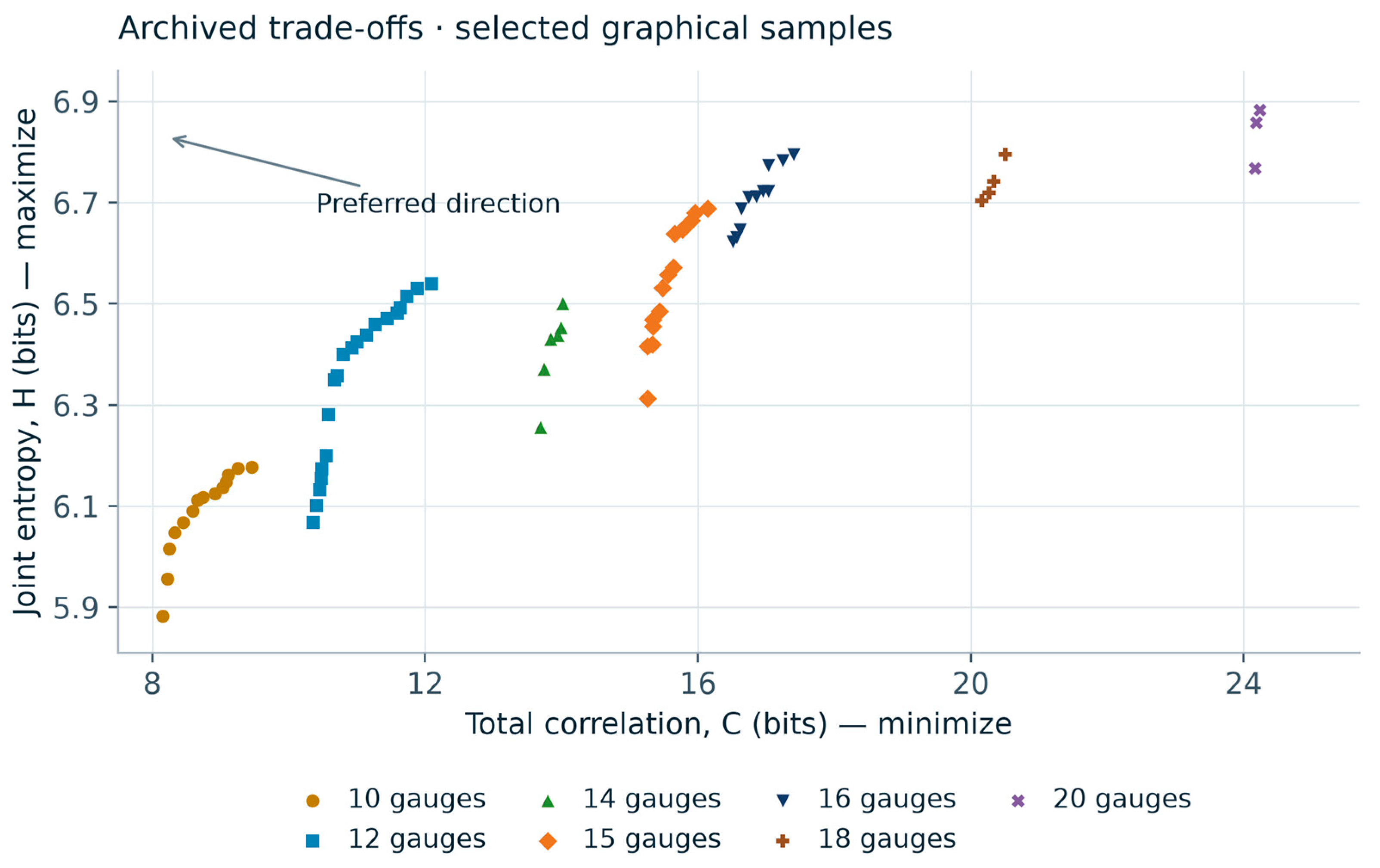
Figure 5 displays 72 selected markers transcribed from the objective-space plot in [13]. Increasing H is displayed upward, while increasing C is displayed to the right; the original station-count groups are retained. Within a group, the upper-left direction indicates the desired combination of greater information and lower dependence. This graphical illustration complements the numerical network-size comparisons in Figure 3 and Figure 4.
Figure 5.
Information–dependence trade-offs illustrated by selected markers graphically transcribed from [13]. Station-count labels are retained from the source and coordinates are approximate. The upper-left direction indicates larger H and smaller C. This descriptive panel illustrates objective-space geometry; the information-retention percentages in Figure 3 and Figure 4 are calculated separately from the reported entropy values.
3.3. Spatial Representation of Annual Rainfall
Figure 7 compares the annual-rainfall contours produced by the proposed 16-site configuration with the CPRM reference reproduced in [13]. Both maps show broad spatial organization of rainfall across the basin, including contour curvature in its central and southern portions. Local contour positions differ, so the comparison is used to examine spatial representation at the map scale. It complements the entropy criterion by showing the rainfall field associated with the proposed arrangement.
3.4. Spatial Distribution and Interpretation of VOI
Figure 8 displays an illustrative VOI surface reconstructed from the five classes mapped for the 101 candidate locations in the Rio das Velhas analysis [13]. The source classes span 14.03–22.79 on the scale of the adopted hypothetical consequences. The interpolated field and its three-dimensional view make the geographic variation in the mapped classes easier to examine. Higher-class locations occur in several parts of the basin, interspersed with lower-class locations, showing that decision relevance varies across the candidate set under this model.
The mapped classes summarize the decision model used in the original network study. In that formulation, observations at a monitoring site can inform decisions at other locations [13]. Figure 8 visualizes the geographic distribution of the resulting candidate-site scores through class midpoints. The peaks and depressions therefore represent the mapped score pattern, while the interpolated areas provide a continuous visual connection between sites. This spatial view complements the entropy comparisons by showing where the adopted decision context assigns greater value to information.
3.5. Analytical Results for the Hypothetical Decision Model
For the hypothetical utilities in Table 1, let p be the probability of the low-rainfall state. Expected utility equals 25p − 30 for preventive action and −100p for no action. The actions are equivalent at p = 0.24, and prevention is preferred above this threshold. With perfect state information, expected utility is −5p. The resulting value of perfect information is 95p for p ≤ 0.24 and 30(1 − p) otherwise, reaching a maximum of 22.8 utility units per decision.
Figure 9 shows that information has its greatest potential value near the probability at which the preferred action changes. At the extremes, where one rainfall state is nearly certain, the potential benefit declines. Under this hypothetical model, the perfect-information curve provides an upper bound on EVSI and a reference for assessing how effectively observations resolve a consequential decision.
3.6. Worked Example with Imperfect Observations
To illustrate EVSI, assume a prior probability of low rainfall of 0.20 and a monitoring message that reports danger with probability 0.80 under low rainfall and 0.20 under high rainfall. These message probabilities are illustrative assumptions, used with the hypothetical utilities in Table 1. Before observing a message, expected utilities are −25 for preventive action and −20 for no action, so the preferred initial decision is no action.
The probability of a danger message is 0.32, and Bayes’ rule gives a posterior low-rainfall probability of 0.50. A normal message has probability 0.68 and a posterior low-rainfall probability of approximately 0.0588. The optimal policy is therefore to take preventive action after danger and no action after a normal message. Averaging the corresponding utilities gives −9.6, an improvement of 10.4 over the initial expected utility of −20.
Perfect information would yield an expected utility of −1.0 and a value of 19.0, so the imperfect-message EVSI remains below its perfect-information bound (Table 2). The example demonstrates the contribution of message reliability: observations improve expected utility by allowing different actions for different messages. These are analytical values for the stated scenario.
3.7. Sensitivity to Priors Message Performance and Consequences
The sensitivity analysis identifies a finite range of prior conditions in which observations change the action. At q = 0.80, the interval is 0.0732 < p < 0.5581 (Figure 10a). At smaller priors both messages lead to no action; at larger priors both lead to prevention. For a fixed q, EVSI reaches its maximum at t = 0.24, where the two actions have equal prior expected utility. The maximum is 22.8(2q − 1), equal to 13.68 utility units at q = 0.80.
At p = 0.20, Equation (12) reduces to EVSI = max{0, 43q − 24}. Positive decision benefit therefore requires q > 24/43, approximately 0.5581 (Figure 10b). Reliability values of 0.60, 0.80 and 0.90 yield 1.8, 10.4 and 14.7 utility units, respectively. Each 0.10 increase in q above this threshold adds 4.3 utility units under the specified model, up to the perfect-information bound of 19.0. In the asymmetric case, Equation (13) requires 19α > 24β (Figure 10d), exposing the separate contributions of detection and false alarms.
Information gain and decision benefit follow different response curves (Figure 10c). At p = 0.05 and q = 0.80, the message supplies 0.0561 bits of mutual information, resolving approximately 19.6% of the binary-state entropy. Its danger-message posterior is only 0.1739, below the action threshold, so EVSI remains zero. At p = 0.20 with the same q, mutual information is 0.1825 bits and EVSI is 10.4 utility units, or 54.7% of EVPI. Thus, resolving uncertainty produces decision value when it changes an action whose consequences differ across rainfall states.
Consequence sensitivity changes both the preferred prior action and the value of the same observation (Table 3). At p = 0.20 and q = 0.80, changing the false-alarm loss b from 15 to 30 to 60 gives EVSI values of 5.8, 10.4 and 5.6 utility units. The response is non-monotonic because b changes the action threshold and the prior decision, in addition to the consequences of a message. A monitoring requirement should therefore specify the decision context together with observation reliability.
4. Discussion
4.1. Information Efficiency and Decision Relevance
The reported configurations reveal a strong concentration of the reference entropy in a smaller monitoring network: 15 of the 28 internal stations retain 90.8% of the reported value. The comparison provides a quantitative basis for screening alternatives when network size is constrained. The smaller entropy differences per station across larger configurations also make the trade-off visible, helping planners identify alternatives that retain substantial information before applying operational and decision-specific criteria.
The analytical results explain why information retention and decision relevance need distinct assessment. At p = 0.05, the assumed monitoring message reduces uncertainty but leaves both posterior-optimal actions unchanged. At p = 0.20, the same reliability changes the preferred action after danger and yields EVSI = 10.4. This difference arises from the position of the posterior probabilities relative to the action threshold. The comparison therefore identifies a mechanism linking monitoring performance to consequences, beyond the amount of statistical information conveyed.
For rainfall-network planning, the derived thresholds translate a decision model into performance requirements. A proposed observation system must distinguish relevant states well enough to move the posterior across the action boundary. Under the baseline prior and consequences, symmetric reliability must exceed 0.5581; asymmetric messages must satisfy 19α > 24β. These requirements can be used to assess candidate observation or forecasting products once their event-detection performance has been estimated for the intended decision horizon [7,8].
4.2. Dependence and Spatial Representation
Total correlation identifies multivariate dependence among station observations and complements joint entropy in network comparison. Its interpretation depends on monitoring objectives: some redundancy can support fault detection, continuity and observation of rare events. A useful design assessment therefore considers the information retained by a compact configuration together with the operational functions of individual stations.
The spatial formulation connects these information criteria with decision locations and their relative importance. Joint observation models account for overlapping evidence, and spatial weights can represent area, exposure or management priorities. Candidate networks derived from interpolation must also be interpreted in relation to the spatial representation supplied by the original gauges [2,5]. Together, these elements define how the framework can be adapted to a specified monitoring and decision problem.
The annual-rainfall overlay provides a complementary view of what a compact configuration represents geographically. Its comparison across different reference periods is useful for assessing broad contour organization, while event reconstruction and predictive accuracy require temporally aligned observations. The VOI surface serves a different purpose: it displays the mapped decision-value classes under the source consequence model. Rainfall contours, entropy ratios and VOI therefore answer separate questions about spatial representation, statistical information and action-dependent benefit.
4.3. Implications for Monitoring Design
The 15-station configuration provides a practical reference for comparing information retention and network size: it preserves more than 90% of the reference entropy with 13 fewer stations. The 10- and 12-station alternatives make the same balance explicit at smaller network sizes. This comparison can help prioritize configurations for planning, with the preferred alternative depending on spatial coverage, monitoring continuity and the intended use of rainfall observations.
A practical application can first identify configurations that satisfy an information-retention target and operational constraints, then evaluate their message performance for a specified management decision. Among feasible alternatives, VOI measures the expected improvement relative to acting with prior information alone. The threshold analysis also helps identify contexts in which improving a monitoring product is unlikely to change the current action, or where a modest improvement in reliability can make an observation useful.
The contribution complements uncertainty-aware entropy design [5] and recent approaches that combine information measures with spatial and temporal prediction [11,12]. Here, the added analytical results make the action-switching conditions and information–value distinction explicit within a rainfall-network application. The reported network comparisons, graphical spatial reconstructions and hypothetical decision scenarios retain their respective scales of interpretation. Empirical transfer of the derived thresholds requires event probabilities and consequences appropriate to the management problem.
5. Conclusions
The Rio das Velhas results identify compact rainfall-network configurations that retain a substantial share of the reference joint entropy. The 15-station configuration retains 6.62 of 7.29 bits (90.8%) with 46.4% fewer stations, while the 10-station configuration retains 85.6% with 64.3% fewer stations. The proposed 16-site candidate arrangement and its annual-rainfall contours add spatial context to the information-based comparison.
The decision analysis establishes explicit conditions under which observations generate value. Under the stated utility model, q = 0.80 produces positive EVSI for priors between 0.0732 and 0.5581. At p = 0.20, EVSI is 10.4 utility units and becomes positive only above symmetric reliability 0.5581. The asymmetric condition 19α > 24β expresses the corresponding balance between event detection and false alarms. These results turn the decision criterion into a quantitative performance requirement.
Information gain alone does not determine decision benefit. At p = 0.05 and q = 0.80, the message resolves 0.0561 bits of uncertainty while EVSI remains zero because the preferred action is unchanged. This result supports a two-stage design logic: use entropy and dependence to identify informative network alternatives, then use explicit decisions, probabilities and consequences to assess their value. The framework connects compact network design with the conditions under which monitoring can improve management choices.
References
- Mishra, A.K.; Coulibaly, P. Developments in hydrometric network design: A review. Rev. Geophys. 2009, 47, RG2001. [Google Scholar] [CrossRef]
- Keum, J.; Kornelsen, K.C.; Leach, J.M.; Coulibaly, P. Entropy Applications to Water Monitoring Network Design: A Review. Entropy 2017, 19, 613. [Google Scholar] [CrossRef]
- Shannon, C.E. A Mathematical Theory of Communication. Bell Syst. Tech. J. 1948, 27, 379–423. [Google Scholar] [CrossRef]
- Li, C.; Singh, V.P.; Mishra, A.K. Entropy theory-based criterion for hydrometric network evaluation and design: Maximum information minimum redundancy. Water Resour. Res. 2012, 48, W05548. [Google Scholar] [CrossRef]
- Keum, J.; Awol, F.S.; Ursulak, J.; Coulibaly, P. Introducing the Ensemble-Based Dual Entropy and Multiobjective Optimization for Hydrometric Network Design Problems: EnDEMO. Entropy 2019, 21, 947. [Google Scholar] [CrossRef]
- Howard, R.A. Information Value Theory. IEEE Trans. Syst. Sci. Cybern. 1966, 2, 22–26. [Google Scholar] [CrossRef]
- Alfonso, L.; Price, R. Coupling hydrodynamic models and value of information for designing stage monitoring networks. Water Resour. Res. 2012, 48, W08530. [Google Scholar] [CrossRef]
- Alfonso, L.; Mukolwe, M.M.; Di Baldassarre, G. Probabilistic Flood Maps to support decision-making: Mapping the Value of Information. Water Resour. Res. 2016, 52, 1026–1043. [Google Scholar] [CrossRef]
- Pádua, L.H.R.; Nascimento, N.O.; Silva, F.E.O.; Alfonso, L. Analysis of the fluviometric network of Rio das Velhas using Entropy. RBRH 2019, 24, e42. [Google Scholar] [CrossRef]
- Bertini, C.; Ridolfi, E.; de Padua, L.H.R.; Russo, F.; Napolitano, F.; Alfonso, L. An entropy-based approach for the optimization of rain gauge network using satellite and ground-based data. Hydrol. Res. 2021, 52, 620–635. [Google Scholar] [CrossRef]
- Liu, J.; Li, Y.; Wang, Y.; Xu, P. Utilizing Entropy-Based Method for Rainfall Network Design in Huaihe River Basin, China. Water 2023, 15, 3115. [Google Scholar] [CrossRef]
- Huang, Y.; Lu, X.; Luo, H.; Liu, B.; Wang, R. A Novel Optimal Layout Method for Rain Gauge Network Based on Mutual Information Entropy and Deep Learning Model. Sensors 2026, 26, 3532. [Google Scholar] [CrossRef]
- Pádua, L.H.R. Análise de redes hidrométricas em bacias brasileiras utilizando teoria da informação e valor da informação. Tese de doutorado, Universidade Federal de Minas Gerais, Belo Horizonte, Brasil, 2020. [Google Scholar]
- Paninski, L. Estimation of Entropy and Mutual Information. Neural Comput. 2003, 15, 1191–1253. [Google Scholar] [CrossRef]
- Deb, K.; Pratap, A.; Agarwal, S.; Meyarivan, T. A fast and elitist multiobjective genetic algorithm: NSGA-II. IEEE Trans. Evol. Comput. 2002, 6, 182–197. [Google Scholar] [CrossRef]
Figure 1.
Framework linking rainfall observations, candidate networks, information criteria and decision value. The independent-evaluation stage is proposed for subsequent assessment.
Figure 1.
Framework linking rainfall observations, candidate networks, information criteria and decision value. The independent-evaluation stage is proposed for subsequent assessment.
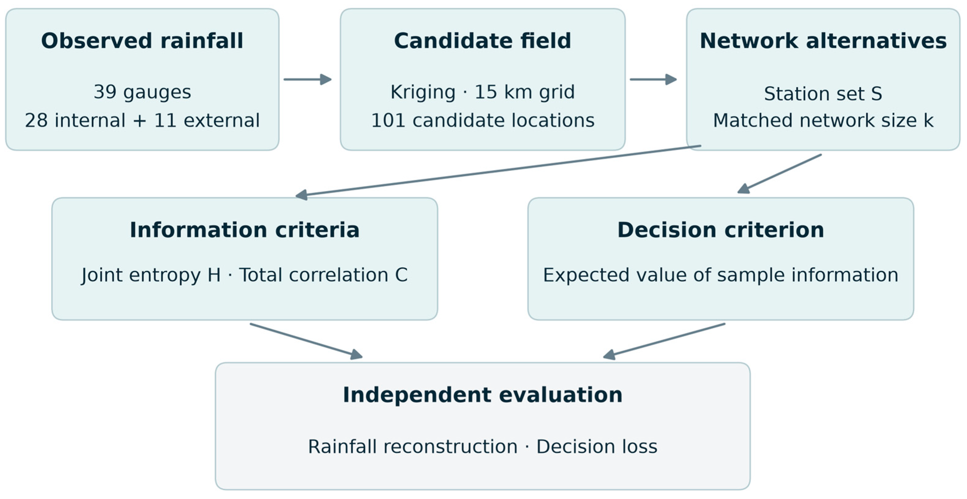
Figure 2.
Candidate locations in the Rio das Velhas basin, reproduced from ([13] Figure 4.11). Red points indicate candidate sites, blue lines the river network, and the black outline the basin boundary. Original cartographic labels and source attribution are retained.
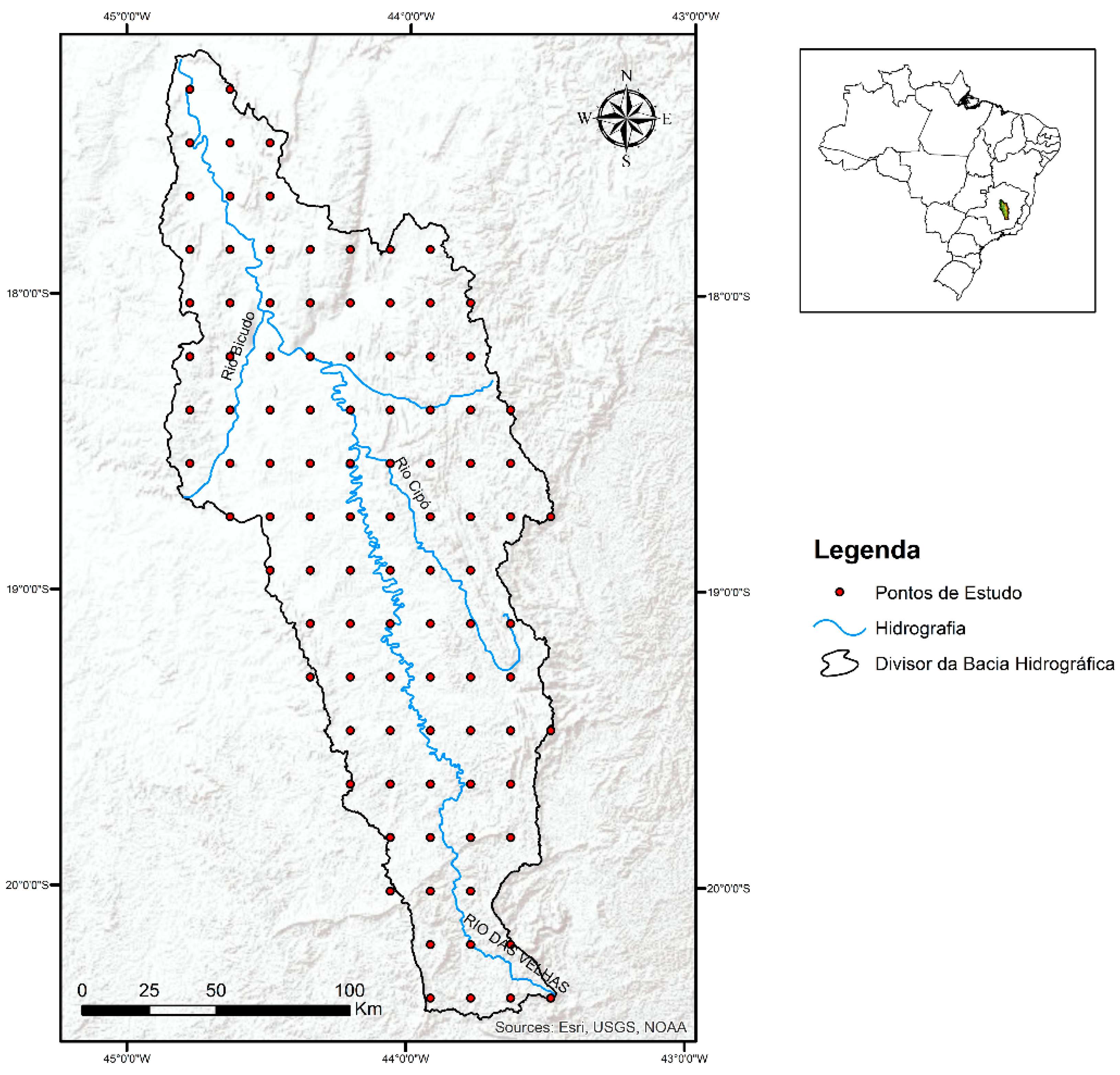
Figure 3.
Joint entropy of existing-network configurations relative to the 28-gauge reference of 7.29 bits, using the values reported in [13]. Labels show entropy and the corresponding percentage; the dashed line marks the 90% criterion.
Figure 3.
Joint entropy of existing-network configurations relative to the 28-gauge reference of 7.29 bits, using the values reported in [13]. Labels show entropy and the corresponding percentage; the dashed line marks the 90% criterion.
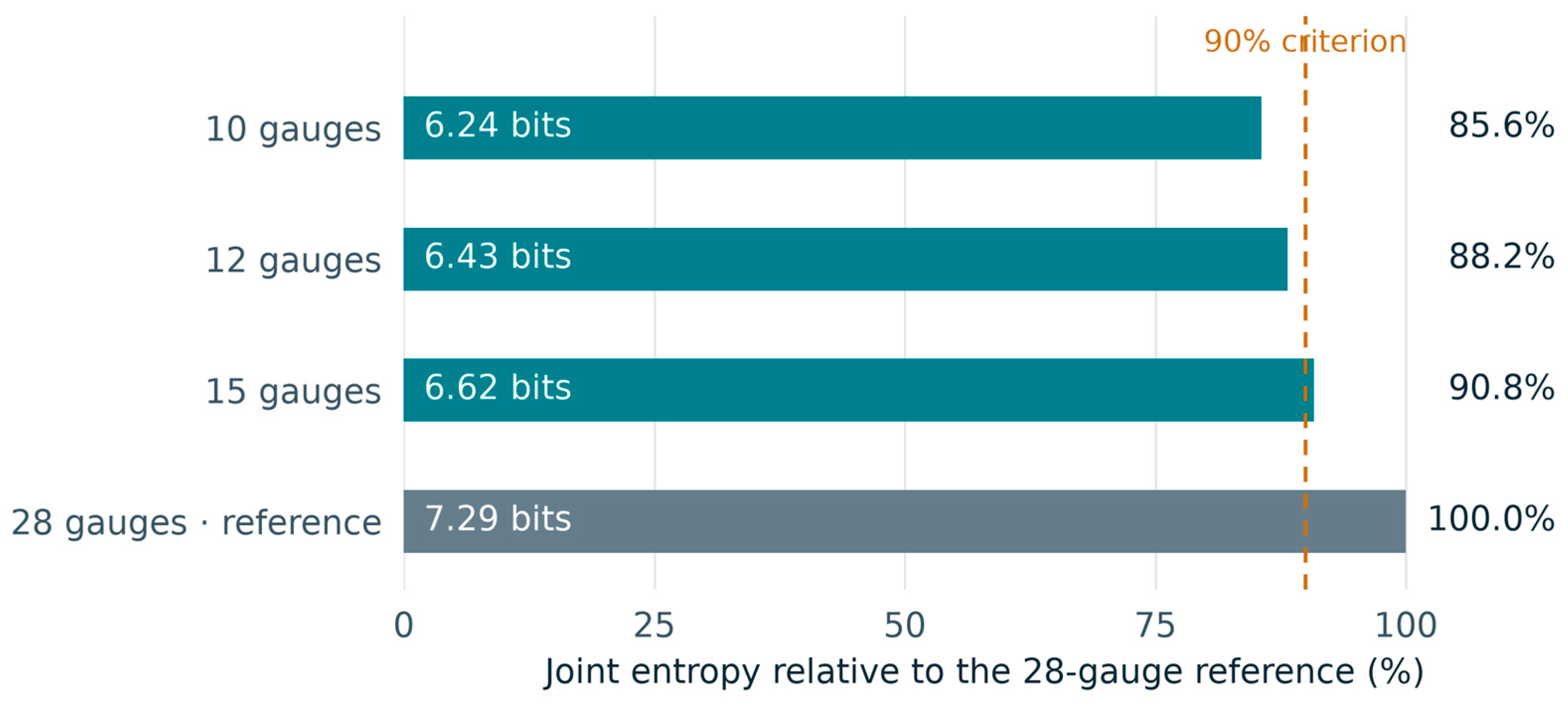
Figure 4.
Network-size trade-offs calculated from the reported existing-network values [13]. (a) Information retained versus reduction in station count relative to the 28-gauge reference; the dashed line marks 90%. (b) Difference in joint entropy divided by the difference in station count for each pair of configurations.
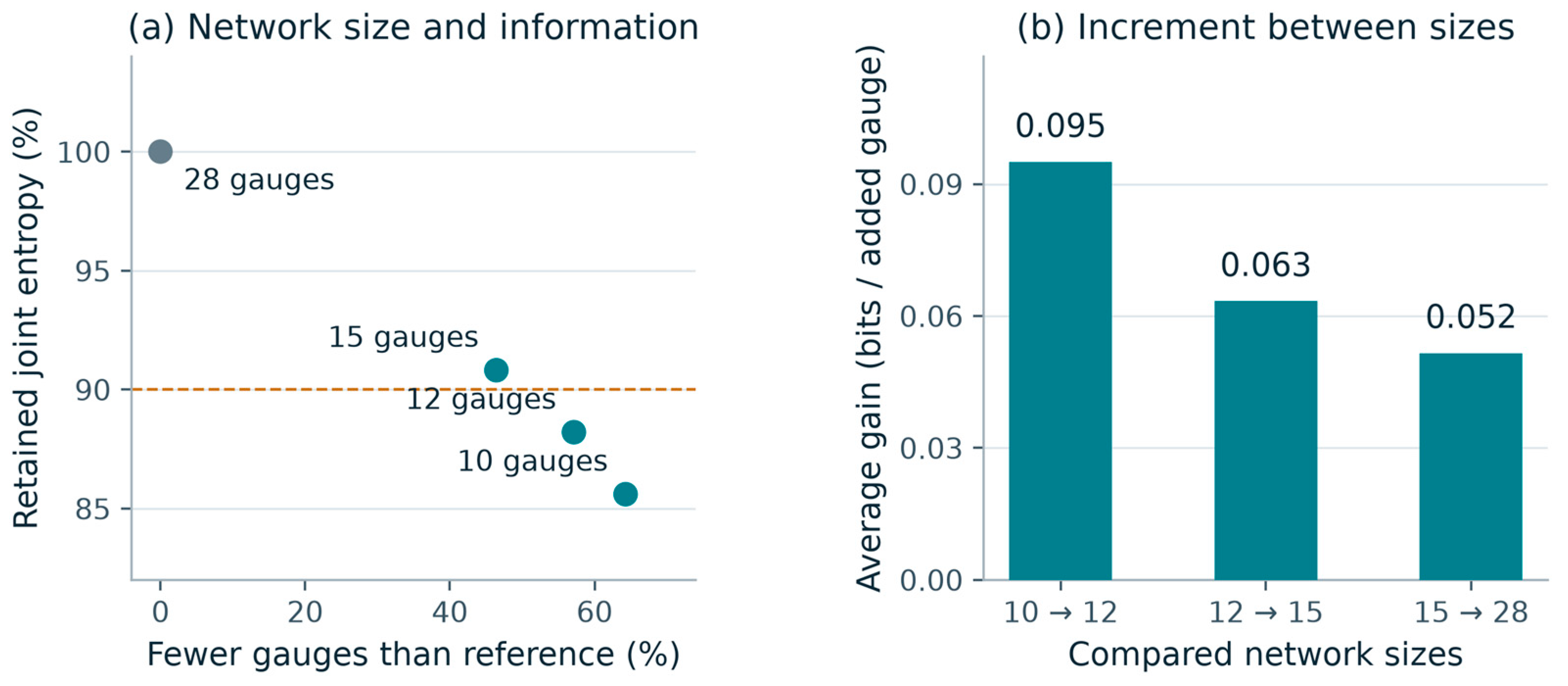
Figure 6.
Proposed 16-station configuration, reproduced from ([13] Figure 5.26). Red triangles indicate proposed gauges and green circles indicate existing gauges. Original cartographic labels and attribution are retained.
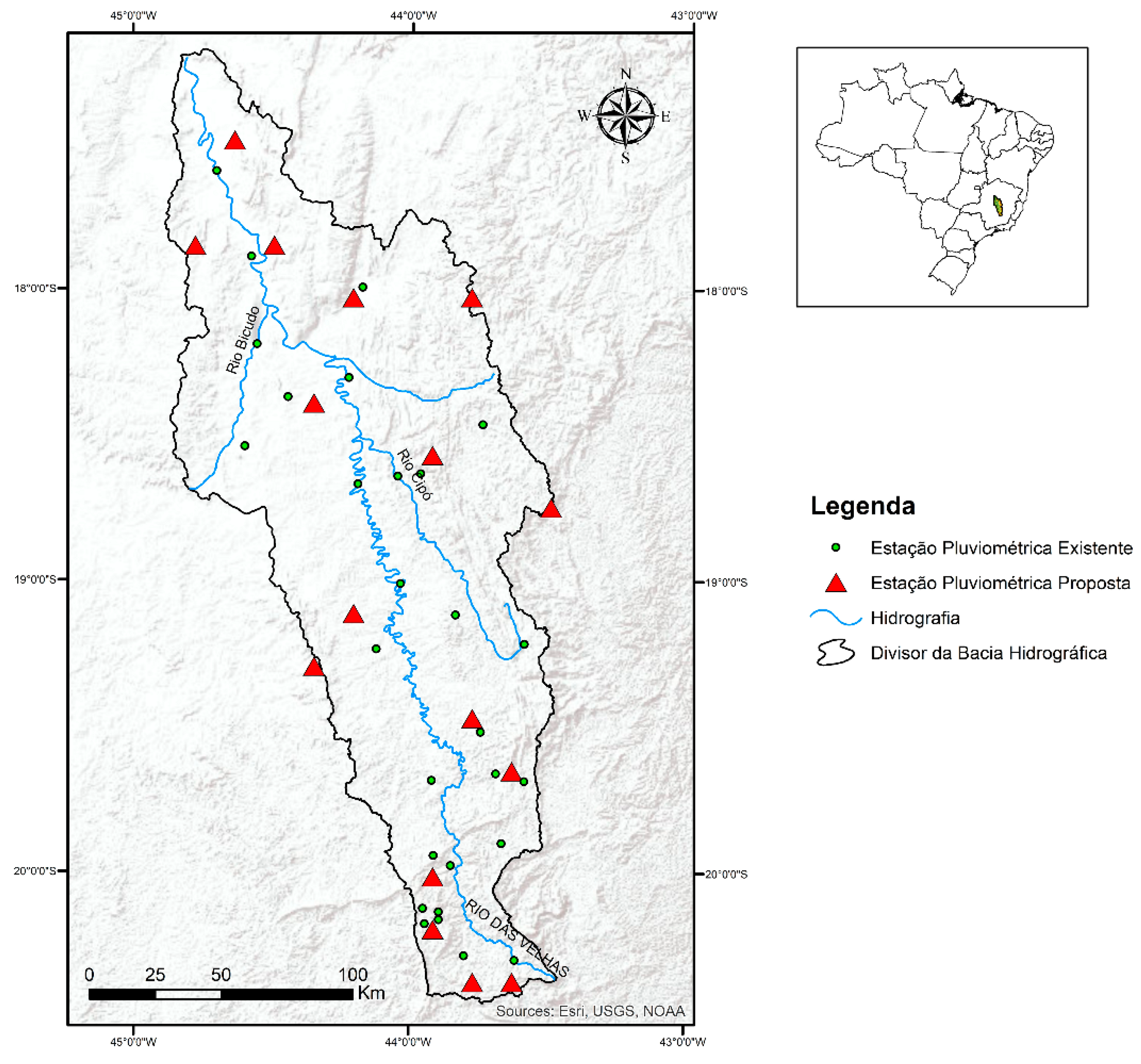
Figure 7.
Annual-rainfall contour comparison for the proposed 16-site configuration, reproduced from ([13] Figure 5.27). Red contours represent the proposed network and green contours the CPRM reference labelled 1977–2006. The observation interval reported for the network study is 1994–2014. The overlay provides a qualitative comparison of broad spatial structure across these periods. Original cartographic labels and attribution are retained.
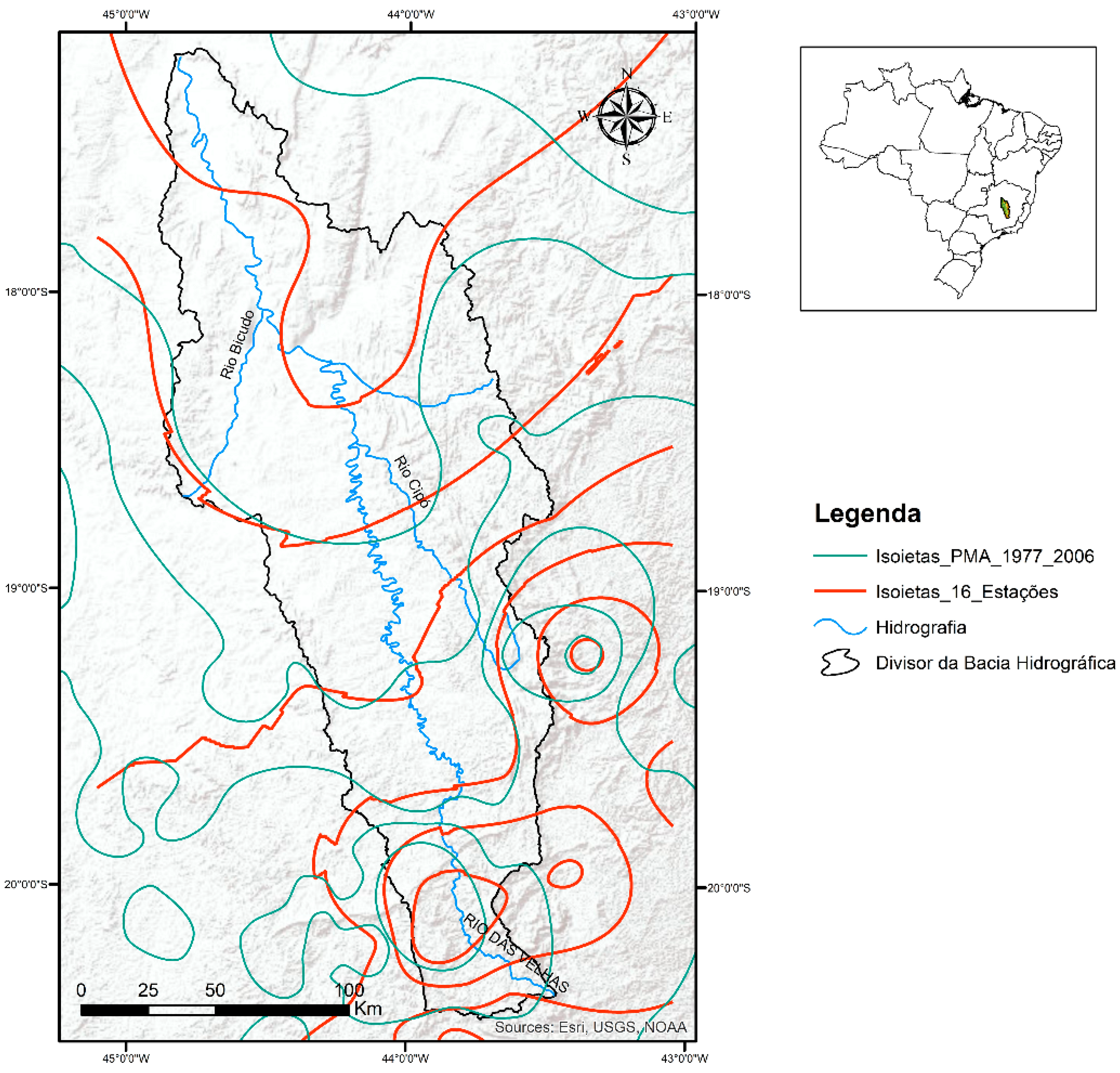
Figure 8.
Illustrative VOI surface reconstructed from the five classes in ([13] Figure 5.28). (a) Interpolated field, isolines and 101 digitized candidate locations (open circles). (b) Three-dimensional view of the same field. Heights represent class midpoints interpolated by inverse-distance weighting (power 2); coordinates and the basin outline were digitized from the source map. The shared color scale retains the original class range. The surface visualizes decision-value classes, not terrain elevation or exact station scores.
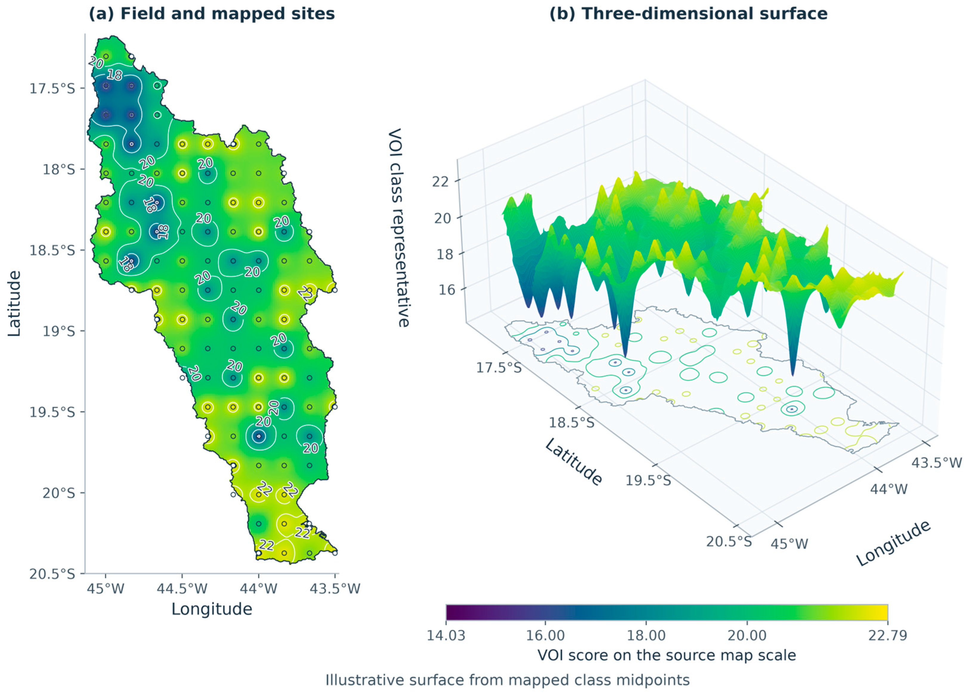
Figure 9.
Analytical results for the hypothetical utility matrix in Table 1. (a) Expected utilities intersect at p = 0.24; preventive action is preferred above that probability. (b) Perfect-information value peaks at 22.8 utility units per decision and provides an upper bound on EVSI under the stated model.
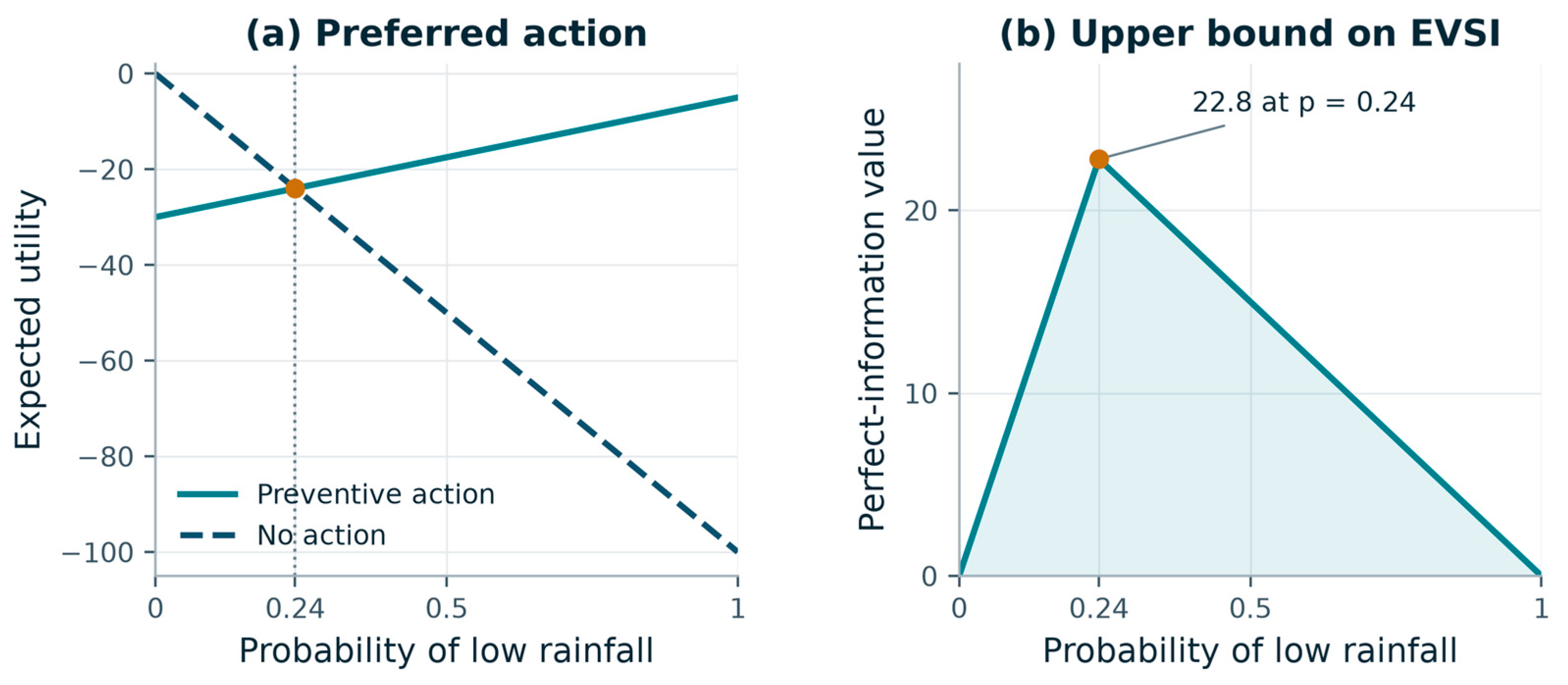
Figure 10.
Analytical sensitivity of the hypothetical decision model. (a) EVSI over prior probability p and symmetric reliability q; solid white curves delimit the positive-value interval, and the dotted line marks t = 0.24. (b) EVSI at p = 0.20. (c) Mutual information normalized by binary-state entropy and EVSI normalized by EVPI, as q varies from 0.5 to 1; markers identify q = 0.80 and the dotted diagonal denotes equal fractions. (d) EVSI at p = 0.20 for asymmetric sensitivity α and false-alarm rate β; the white line is the zero-benefit boundary 19α = 24β. Orange markers in (a), (b) and (d) identify the worked example. Probabilities are scenario assumptions.
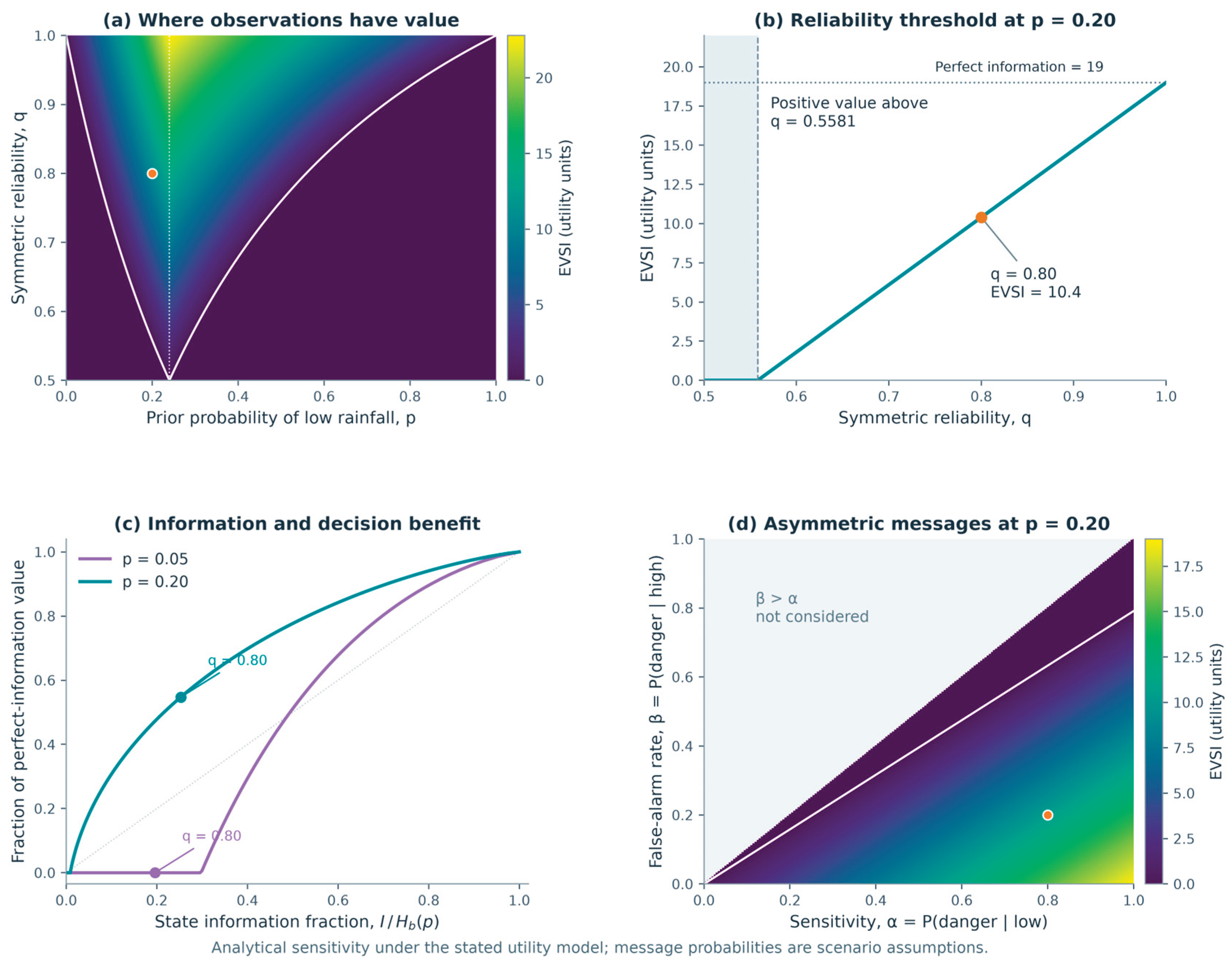

Table 1.
Hypothetical utilities for the decision example, adapted from ([13] Table 4.10).
Table 1.
Hypothetical utilities for the decision example, adapted from ([13] Table 4.10).
| Action | Low rainfall state | High rainfall state |
|---|---|---|
| Preventive action | −5 | −30 |
| No action | −100 | 0 |
Table 2.
Expected utility and VOI in the illustrative imperfect-information example. Prior low-rainfall probability is 0.20; the danger-message likelihoods are 0.80 under low rainfall and 0.20 under high rainfall. Values use the utility scale in Table 1.
Table 2.
Expected utility and VOI in the illustrative imperfect-information example. Prior low-rainfall probability is 0.20; the danger-message likelihoods are 0.80 under low rainfall and 0.20 under high rainfall. Values use the utility scale in Table 1.
| Information case | Optimal policy | Expected utility | VOI |
|---|---|---|---|
| No new information | No action | −20.0 | 0.0 |
| Imperfect messages | Prevent after danger; no action after normal | −9.6 | 10.4 |
| Perfect information | Prevent under low rainfall; no action under high rainfall | −1.0 | 19.0 |
Table 3.
Sensitivity to the loss b of preventive action under high rainfall. All cases use p = 0.20, q = 0.80, prevention loss under low rainfall c = 5 and unmitigated low-rainfall loss L = 100. Values are hypothetical utility losses, not monetary estimates for the basin.
Table 3.
Sensitivity to the loss b of preventive action under high rainfall. All cases use p = 0.20, q = 0.80, prevention loss under low rainfall c = 5 and unmitigated low-rainfall loss L = 100. Values are hypothetical utility losses, not monetary estimates for the basin.
| False-alarm loss b | Action threshold t | Action before message | EVSI |
|---|---|---|---|
| 15 | 0.1364 | Prevention | 5.8 |
| 30 | 0.2400 | No action | 10.4 |
| 60 | 0.3871 | No action | 5.6 |
Disclaimer/Publisher’s Note: The statements, opinions and data contained in all publications are solely those of the individual author(s) and contributor(s) and not of MDPI and/or the editor(s). MDPI and/or the editor(s) disclaim responsibility for any injury to people or property resulting from any ideas, methods, instructions or products referred to in the content. |
© 2026 by the authors. Licensee MDPI, Basel, Switzerland. This article is an open access article distributed under the terms and conditions of the Creative Commons Attribution (CC BY) license (http://creativecommons.org/licenses/by/4.0/).
Copyright: This open access article is published under a Creative Commons CC BY 4.0 license, which permit the free download, distribution, and reuse, provided that the author and preprint are cited in any reuse.