

Submitted:
08 October 2026
Posted:
09 October 2026
You are already at the latest version
Abstract
State policy shocks are routinely capitalised into housing markets, yet the spatial resolution at which that capitalisation can be observed is rarely tested. This study examines the 2022 Dobbs v. Jackson Women’s Health Organization decision, after which thirteen United States states enacted total abortion bans. Replicating and extending county-level synthetic difference-in-differences estimates by one year, rents in ban states remain 2.9% below their synthetic counterfactual through June 2026 and home values 2.3% below, although rent significance depends on the state-level variance estimator. The study then asks whether the decline concentrates in the neighbourhoods where women of reproductive age cluster. A within-metropolitan two-way fixed-effects design across 337 ZIP codes in thirteen ban-state metropolitan areas returns a −0.86% differential that fails its parallel-trends test, depends on a single state and loses significance once spatial dependence is respected: spatially blocked randomisation inference yields p = 0.224, against p = 0.022 when ZIP codes are permuted individually. The exposure measure is spatially clustered (Moran’s I = 0.125) and 46.4% predicted by density, income, age and tenure, so it locates neighbourhoods on the urban gradient rather than isolating policy exposure. A sex-composition test nearly orthogonal to that gradient returns an informative null, excluding differentials beyond ±1%, and the same gradient moved rents in protecting-state metropolitan areas where no policy changed. Capitalisation detectable across states need not be recoverable within cities; compositional neighbourhood measures require explicit specificity and spatial-inference tests before they inform local planning or underwriting.
Keywords:
spatial scale
; residential sorting
; spatial autocorrelation
; rental housing
; abortion policy
; difference-in-differences
; randomisation inference
1. Introduction
Place-based policies rarely respect the geography of the markets they disturb. When a legal change is abrupt, follows jurisdictional boundaries and bears on an identifiable population, it operates as a locational shock whose incidence depends on where that population lives (Roback, 1982; Rosen, 1974). Geographers have long warned that such incidence is scale-dependent: relationships observed at one level of aggregation need not hold at another, and inferences drawn across scales risk ecological fallacy (Fotheringham & Wong, 1991; Robinson, 1950). Whether a policy shock measured across states can be resolved within cities is therefore an empirical question about spatial scale, not a matter of statistical detail.
The 2022 United States Supreme Court decision in Dobbs v. Jackson Women’s Health Organization supplies an unusually sharp test. Within weeks, thirteen states enacted total abortion bans, withdrawing reproductive healthcare along state lines that bear no relation to pre-existing housing-market geography. Dench et al. (2026) estimate, with a synthetic difference-in-differences design on county-level Zillow indices, that bans reduced rents by an average of 2.2% between July 2022 and June 2025, interpreting the decline as withdrawal of housing demand by the households for whom reproductive access is most salient.
That interpretation carries a geographical prediction the county design cannot test. If demand withdrawal is concentrated among women of reproductive age, the rent response should be strongest in the neighbourhoods where they cluster. A confirmed concentration would justify treating reproductive-access loss as a localisable disamenity relevant to neighbourhood planning, tenant protection and submarket underwriting; a spurious one would misdirect all three.
The question matters beyond reproductive policy. Housing, planning and investment decisions are increasingly made at submarket resolution, using commercial indices and census-tract or postal-code demographics, while the policy shocks that move those markets are legislated at state or national scale. Inferring neighbourhood incidence from aggregate effects is therefore routine, and rarely tested. Where the population most exposed to a policy is also the population most strongly sorted by density, tenure and age, a neighbourhood contrast risks recovering the sorting rather than the policy.
This study makes three contributions. First, it replicates the county estimate of Dench et al. (2026) and extends it to June 2026. Second, it constructs a within-metropolitan test of the concentration channel across 337 ZIP codes in thirteen ban-state metropolitan areas, with a falsification programme that treats parallel trends as a hypothesis, isolates neighbourhood sex composition from the general concentration of young adults and respects spatial dependence in inference. Third, it shows that a compositional exposure measure inherits the urban gradient produced by residential sorting (Couture & Handbury, 2020; Diamond, 2016), a hazard general to applied neighbourhood analysis. Section 2 reviews the literature; Section 3 sets out data and methods; Section 4 reports results; Section 5, Section 6, Section 7 and Section 8 discuss limitations, implications and conclusions.
2. Literature and Conceptual Framework
Four literatures discipline the design: the capitalisation of place-based attributes and its dependence on scale; reproductive policy as a locational disamenity; residential sorting as both precondition and confound; and inference under spatial dependence with few clusters.
1.1. Capitalisation, Scale and the Ecological Trap
Hedonic and spatial-equilibrium theory implies that any attribute altering the desirability of a place, including legal and healthcare conditions, is capitalised into rents and property values as households re-sort (Roback, 1982; Rosen, 1974). The best-quantified evidence concerns environmental disamenities: housing-value elasticities of −0.20 to −0.35 with respect to particulates (Chay & Greenstone, 2005), a 4.4–5.5% rent discount near fossil-fuel power plants (Davis, 2011) and localised discounts around toxic plants (Currie et al., 2015). Legal rights can operate similarly. The presence of same-sex couples carries a premium in liberal neighbourhoods and a discount in conservative ones (Christafore & Leguizamon, 2012), and state-level legalisation of same-sex marriage redirected interstate migration until national legalisation removed the locational advantage (Marcén & Morales, 2022).
Capitalisation is heterogeneous: willingness to pay varies with income, education and household composition, so aggregate estimates average over sorted populations (Bayer et al., 2007; Kuminoff et al., 2013). This heterogeneity tempts analysts to move from aggregate effects to neighbourhood mechanisms by correlating outcomes with local composition. Geography offers two warnings. Aggregate associations do not license individual-level or finer-scale inference (Robinson, 1950), and estimated relationships change with the size and configuration of the spatial units used (Fotheringham & Wong, 1991). For policy evaluation the implication is specific: an effect identified across states is a statement about the state as a unit, and its decomposition across neighbourhoods is a separate empirical claim requiring its own identification. A third concerns context: a ZIP code’s demographic composition is an imperfect proxy for the environment that shapes its residents’ choices (Kwan, 2012).
1.2. Reproductive Policy as a Locational Disamenity
Dench et al. (2026) supply the anchor estimate: alongside the rent decline, bans raised rental vacancy. Companion evidence from postal change-of-address records shows net outflows from ban states, larger for single-person households (Dench, Lifchez, et al., 2025), with fertility effects scaling with the change in driving distance to the nearest provider (Dench, Myers, & Pineda-Torres, 2025). Nelson and Witko (2026) corroborate a modest interstate migration response, which motivates a within-metropolitan test where adjustment need not clear the cost of an interstate move. The micro-foundations are established: reproductive control shapes the timing of family formation and labour supply (Bailey, 2006; Myers, 2017), abortion denial raises poverty and financial distress (Foster et al., 2018; Miller et al., 2023), and greater travel distance raises housing insecurity (Aslim et al., 2025; Lindo et al., 2020). Health stakes are documented, including excess infant deaths in Texas after its 2021 restriction (Gemmill et al., 2024), and most surveyed physicians and trainees prefer to practise in access-preserving states (Bernstein et al., 2023).
One consideration bounds the expected neighbourhood signal. Telehealth-dispensed medication abortion grew rapidly after 2022 and, by 2025, accounted for nearly all abortions provided within ban states, while interstate travel for care declined (Maddow-Zimet & Forouzan, 2026; Society of Family Planning, 2026). Because this substitute is available irrespective of residential location, it attenuates the specifically local component of the disamenity, leaving travel fallback, legal risk and provider availability as the residual that could be capitalised by neighbourhood.
1.3. Residential Sorting: Precondition and Confound
A within-metropolitan test has power only if the affected population clusters in identifiable, segmented submarkets. The sorting literature shows that it does. College-educated adults aged 25–34 drove the post-2000 revival of American city centres, with downtowns holding about 5% of metropolitan population absorbing close to a quarter of the growth in young graduates across the largest metropolitan areas (Couture & Handbury, 2020); skill sorting across metropolitan areas is self-reinforcing (Diamond, 2016); and the centrality premium associated with dual-earner households is steeply graded by distance from the centre (Edlund et al., 2022). Submarkets are also imperfectly substitutable: sorting by race and education persists without compensating price differences (Bayer et al., 2007), and within-city house-price dynamics during demand shocks are spatially organised rather than smoothly arbitraged (Guerrieri et al., 2013). Young, educated households are, finally, the most mobile (Molloy et al., 2011).
The same clustering is the design’s principal threat. Neighbourhoods with high shares of women aged 20–39 are, by construction of the sorting process, denser, younger, more renter-occupied and differently priced than the rest of the metropolitan area. Any force moving rents along that gradient, including pandemic-era reallocation away from urban cores, will register as a differential whether or not the policy channel operates. Parallel trends must therefore be tested, and the decisive evidence must come from a dimension of composition that varies independently of the gradient.
1.4. Identification and Inference Under Spatial Dependence
Two-way fixed-effects estimators can be biased under staggered adoption when they compare newly with already-treated units (de Chaisemartin & D’Haultfœuille, 2020; Goodman-Bacon, 2021), motivating heterogeneity-robust alternatives (Callaway & Sant’Anna, 2021; Roth et al., 2023). Inference is a separate problem. Conventional clustered standard errors over-reject with few or unbalanced clusters (Bertrand et al., 2004; Cameron et al., 2008), which wild-cluster bootstraps partly address (Roodman et al., 2019). Spatial dependence compounds the difficulty: when outcomes and treatment are spatially autocorrelated (Moran, 1950), observations nearer than the clustering unit share shocks, and reliable inference requires spatially defined clusters large enough to absorb that dependence (Bester et al., 2011; Conley, 1999). Randomisation inference inherits the same requirement, because permuting spatially clumped labels across individual units breaks the dependence the null distribution should preserve.
1.5. Hypotheses
Figure 1 summarises the causal chain and the rival account the design must distinguish. Two hypotheses are tested two-sided against a null of no within-metropolitan differential.
H1. Within ban-state metropolitan areas, post-Dobbs rent growth in ZIP codes with a high share of women aged 20–39 differs from rent growth in low-share ZIP codes of the same metropolitan area.
H2. Any such differential is specific to the sex composition of the young-adult population and does not merely reflect the concentration of young adults of both sexes.
H2 carries the identifying weight: a differential consistent with H1 is necessary but not sufficient evidence of a reproductive-rights channel, because the exposure measure is entangled with the urban gradient.
3. Data and Methods
Two questions are identified separately. The aggregate question is whether bans moved county rents and home values; the mechanism question is whether any effect concentrates within metropolitan areas. The metropolitan-by-month fixed effects that identify the second remove the first by construction, so a uniform metropolitan repricing of any size leaves the within-metropolitan coefficient at zero.
1.1. Study Area and Data
The outcome is the Zillow Observed Rent Index (ZORI), a smoothed, seasonally adjusted repeat-rent index covering single-family, condominium and multifamily units, reported monthly by ZIP code from January 2015 to June 2026 (Clark, 2022). Exposure is the share of women aged 20–39 in each ZIP code from the 2016–2020 American Community Survey (U.S. Census Bureau, 2024), fixed before the shock; ZIP codes are located at Census ZIP Code Tabulation Area internal points (U.S. Census Bureau, 2025). County ZORI and Zillow Home Value Index (ZHVI) panels support the aggregate replication, deflated by the Consumer Price Index for All Urban Consumers (U.S. Bureau of Labor Statistics, 2026) and classified by the 2023 Rural-Urban Continuum Codes (U.S. Department of Agriculture, 2023).
States are classified following Dench et al. (2026) and Guttmacher Institute (2026) into thirteen ban states, protecting states that preserved or expanded access, and an intermediate tier of gestational limits or delayed bans retained as a graded check. A ZIP code enters only if observed in at least 80% of the 41 pre-treatment months (January 2019 to May 2022), a pre-treatment-only criterion, and if its metropolitan area contains at least six qualifying ZIP codes within one policy tier (Table 1). The filter is not neutral across space. Across the thirteen ban states, 426 of 1,866 Zillow ZIP codes clear it, from 34.2% in Texas to 2.2% in Wisconsin, and retained ZIP codes are two years younger at the median, about $12,000 richer in median household income, 7 percentage points more renter-occupied, 14 points more likely to hold a degree and more than twice as dense as those excluded, and no non-metropolitan county or ZIP code in the Zillow rent files has a single pre-treatment observation, so rural areas cannot enter the rent analysis at any threshold.
Figure 2 maps the exposure split in the four largest ban-state metropolitan areas. High-exposure ZIP codes concentrate in central, contiguous clusters, the spatial structure that later governs inference.
1.2. Within-Metropolitan Design
H1 is estimated by ordinary least squares with ZIP-code and metropolitan-area-by-month fixed effects (Bergé et al., 2026):
ln(ZORI)ᵢₜ = αᵢ + δₘ₍ᵢ₎,ₜ + β (Highᵢ × Postₜ) + εᵢₜ
Highᵢ indicates a female 20–39 share above the metropolitan median; Postₜ is dated to each state’s own effective ban date, between 25 May and 25 August 2022. β is the post-ban change in the within-metropolitan rent gap. Because every comparison is confined to one metropolitan area and month, and hence, except in Memphis (7.7% of metropolitan-month cells), to one state and ban date, no already-treated unit serves as a control; the design lies outside the staggered-adoption critique by its fixed-effects structure, and heterogeneity-robust estimators would discard the within-metropolitan contrast. The preferred window starts in April 2021 to limit pandemic-era composition change; the January 2019 window governs the parallel-trends verdict.
H2 substitutes alternative exposure definitions into the same equation. Candidates are screened by classification agreement, the share of ZIP codes placed on the same side of the metropolitan median as the treatment split, because a placebo can correlate strongly with the treatment measure and still classify almost identically. The discriminating constructs are the female-minus-male share and the female-to-male ratio among 20–39-year-olds. A triple difference adds protecting-state metropolitan areas, matched one-to-one to ban metropolitan areas by number of qualifying ZIP codes (662 ZIP codes):
ln(ZORI)ᵢₜ = αᵢ + δₘ₍ᵢ₎,ₜ + β₁ (Highᵢ × Postₜ) + β₂ (Highᵢ × Postₜ × Banᵢ) + εᵢₜ
The base term β₁, which uses a common post-Dobbs indicator because protecting states have no ban date, measures the exposure gap where no policy changed; β₂, dated to each state’s own ban, is the additional movement in ban metropolitan areas and should be negative under the concentration hypothesis. A three-tier variant adds intermediate states to test whether responses order by restriction severity. Because Texas dominates the ZIP-month sample, the differential is also estimated under equal-metropolitan, within-metropolitan population and resident-population weights, each answering a different question about whose rents moved.
A falsification ladder completes the design: placebo treatment dates before any ban, a specification allowing the exposure gap its own linear trend, a dating-invariance test comparing Texas’s 2021 Senate Bill 8 date with the common post-Dobbs date, leave-one-state and leave-one-metropolitan-area estimates, and exclusion of Memphis, the only metropolitan area spanning two ban cohorts.
1.3. Spatially Aware Inference
Texas supplies 70.6% of ban-tier ZIP codes, so the effective number of state clusters is 1.92 against a nominal seven. State clustering and a Webb-weighted wild-cluster bootstrap are therefore reported but carry little information. The exposure share is spatially autocorrelated within metropolitan areas (ZIP-weighted Moran’s I = 0.125 against a null expectation near −0.04), so the primary procedure permutes high and low labels within each metropolitan area in contiguous 0.25° blocks, preserving geographic clustering. Individual-ZIP permutation, ZIP, metropolitan and spatial-grid clustering at 0.25°, 0.5° and 1.0° are reported for comparison. Nulls are reported with 95% confidence intervals and minimum detectable effects (MDE) at 80% power; a null is informative when its interval excludes effects beyond ±1%, a threshold below the aggregate effect and canonical disamenity benchmarks.
1.4. Aggregate Replication
The replication follows Dench et al. (2026): county panels of ban against protecting states, annual July–June windows, CPI deflation, a common third-quarter 2022 onset and the synthetic difference-in-differences estimator of Arkhangelsky et al. (2021). Because state adoption is genuinely staggered at this level and the ban indicator is constant within a metropolitan month, this estimator, with state-level block-bootstrap and jackknife inference, is used only here.
4. Results
Because the exposure split is a plausible proxy for position on the urban gradient, the parallel-trends test is reported first and governs how every estimate is read.
1.1. Parallel Trends: A Pre-Existing Narrowing
Figure 3 plots the within-metropolitan exposure gap on each state’s event clock. The gap narrows steadily from 2019 and passes through the ban date without a break; the coefficient in the first fully treated month is −0.0007 (p = 0.390). On the January 2019 window the gap narrows by 0.75% a year before the bans (p = 0.004) and 0.38% a year after (p = 0.074): the pre-period trend is roughly twice as steep (Figure 4). The April 2021 window shows no significant pre-trend (p = 0.120) only because it begins after most of the narrowing has occurred. The violation is driven by Texas and, on two metropolitan areas only, Tennessee, both late-adopting states, so it is not an artefact of treatment timing. Texas pre-trends at −0.90% a year (p = 0.005) against −0.35% (p = 0.372) in the remaining ban states, and its break net of trend is positive (+0.0049, p = 0.024), the opposite sign to the hypothesis.
1.2. The Within-Metropolitan Differential (H1)
Table 2 reports the estimates. The unadjusted median split returns −0.86% (95% CI [−1.78, 0.07]); the continuous specification returns −1.72% per ten percentage points of exposure. Both are fragile. Adding renter share, which correlates at 0.625 with exposure and may lie on the causal pathway, reverses the sign to +0.14%, while income adjustment moves the estimate to −1.39%. Weighting metropolitan areas equally, the natural estimand for a within-metropolitan design, yields −0.011% (p = 0.983), and population weighting within metropolitan areas +0.160% (p = 0.713): Texas supplies 70.6% of ZIP codes but only 38.5% of metropolitan areas, so the observation-weighted default largely reports Texas. Excluding Texas gives +0.04% (p = 0.967), on an interval too wide to establish or exclude a Texas-specific effect.
1.3. Falsification: A Trend, Not a Break
Every check designed to separate a break from a trend points to a trend. On the six non-pre-restricted ban metropolitan areas, a placebo dated June 2020, two years before any ban, returns −0.0141 (p < 0.001), larger than the real estimate. Allowing the exposure gap its own linear trend removes the break entirely (+0.0010, p = 0.262). In Texas, dating treatment to September 2021 or July 2022 changes the estimate by 0.00014, the signature of a monotone trend that any post indicator captures. Influence is concentrated by state rather than by place: dropping each metropolitan area in turn leaves the estimate between −0.0116 and −0.0051, whereas dropping Texas moves it to +0.0004. Excluding Memphis changes it by 1%, so cross-cohort contamination is immaterial.
1.4. Spatial Inference Overturns Conventional Significance
Figure 5 subjects the same point estimate to ten inference procedures. Only ZIP-level clustering (p = 0.014) and individual-ZIP permutation (p = 0.022) reach conventional significance, and both treat spatially clustered ZIP codes as independent. Spatial-grid clustering inflates the ZIP-level standard error by 44–80%, and permuting contiguous 0.25° blocks widens the null distribution 1.96-fold, raising the p-value to 0.224. Every spatially or statistically conservative alternative returns p between 0.063 and 0.472. The apparent concentration is, in part, an artefact of ignoring spatial autocorrelation in the exposure measure.
1.5. Specificity: Women or Young Adults? (H2)
Table 3, Panel A, shows why classification agreement matters. The male 20–39 share correlates at 0.741 with the female measure yet classifies 88.7% of ZIP codes identically, so it cannot discriminate between accounts; it returns a larger differential (−1.20%) than the treatment measure. The two sex-composition constructs classify fewer than half of ZIP codes identically, and baseline density, income, age and tenure explain only 3.8% and 4.9% of their within-metropolitan variation, against 46.4% for the exposure split.
Panel B reports the test. All four sex-composition intervals lie within ±1%, with MDEs of 0.44–0.67%, at or below the −0.673% per standard deviation carried by the exposure gradient itself. This is an informative null. Holding male exposure fixed, the female coefficient is +0.18% (p = 0.720); holding female exposure fixed, the male coefficient is −1.34% (p = 0.013), the opposite of the hypothesised ordering. The sex-composition measures show no pre-trend on the pooled ban sample, though they do within Texas, so the null holds for the pooled sample only.
1.6. The Gradient Moves Rents Where No Policy Changed
The triple difference corroborates the gradient account (Figure 6). The base term, the exposure gap among protecting-state metropolitan areas, is significantly negative in three of four specifications (matched sample: −1.07%, p = 0.044). The additional movement in ban metropolitan areas is positive in every specification, opposite to the hypothesis, and never significantly negative; its null is empty rather than precise (matched MDE 1.88%; Figure 6a). Extending the window to January 2019 raises the protecting-metropolitan narrowing to −3.18%, locating about two-thirds of it in 2020, consistent with pandemic reallocation away from dense cores. Nor do responses order by severity: the difference between ban and intermediate tiers ranges from −0.03 to +0.82 percentage points across five specifications (p between 0.182 and 0.951; Figure 6b).
1.7. Aggregate Replication and Extension
Table 4 compares the replication with the published estimates. All three point estimates reproduce to one decimal place, with the home-value county sample matching exactly. Over the extended window to June 2026, rents are 2.87% and home values 2.32% below their synthetic counterfactuals. Single-year estimates share pre-periods and donor pools, so their apparent growth is not formally tested. Rent significance is method-dependent: on the extended window a state block bootstrap excludes zero (95% CI [−5.26, −0.42]) while a state jackknife does not ([−5.91, +0.26]). The home-value interval crosses zero under both, reproducing the published null. Wisconsin and Missouri left the ban group within the window; because synthetic difference-in-differences cannot represent reversal, they are retained as a fixed cohort, and excluding them enlarges the extended effects to −3.47% for rents and −3.21% for home values.
1.8. Rural Coverage and Migration
Two county-level checks address the geography the ZIP design cannot see. Rural rents are unobservable: none of the 110 non-metropolitan counties or 57 non-metropolitan ZIP codes in the Zillow rent files has a pre-treatment observation, the median first observation falling in 2026. Home values are observed, and stratifying the home-value effect by Rural-Urban Continuum Code returns −1.92% in metropolitan counties, −2.37% in adjacent non-metropolitan counties and −0.71% in remote rural counties, the last an empty null (MDE 2.18%) and the non-metropolitan estimates largely driven by Texas. The gradient is therefore not ordered towards rural areas, contrary to a travel-distance account, but cannot be ruled out. County net migration from Census population estimates narrowed the ban-minus-protecting gap by 4.84 migrants per 1,000 residents after 2022 (95% CI [−7.38, −2.30]), concentrated in metropolitan counties and robust to excluding Texas; with only two pandemic-era pre-treatment years, this corroborates the direction of the rent result without identifying it.
5. Discussion
Two findings, estimated at different spatial resolutions, coexist without contradiction. The association between total bans and county rents is real, reproducible and persistent. The mechanism most naturally proposed to explain it, demand withdrawal concentrated where women of reproductive age live, cannot be separated from a pre-existing urban rent gradient at the neighbourhood scale. Three results support this reading rather than assume it: the gap was narrowing faster before the bans than after; it narrowed where no policy changed; and the one measure orthogonal to the gradient returns a precise null.
The broader lesson is geographical. A compositional exposure measure is also a measure of position on the urban gradient, because the sorting processes that concentrate a policy-relevant population also concentrate density, tenure, income and age. A within-city contrast on such a measure will tend to show apparent concentration whether or not the hypothesised channel operates, a scale-specific variant of the ecological problem identified by Robinson (1950) and of the context problem described by Kwan (2012). Spatial autocorrelation sharpens the hazard: because exposure is clumped, inference that treats neighbourhoods as independent manufactures significance. The remedies demonstrated here transfer to other place-based shocks, including climate-risk disclosure, school rezoning and policing changes: screen placebos by classification agreement rather than correlation, seek a dimension of exposure orthogonal to the gradient, report equal-area as well as observation-weighted estimands, and block permutations spatially.
The results also qualify the aggregate interpretation. Because the fixed effects remove uniform metropolitan repricing, the neighbourhood null is evidence against localised concentration, not against the aggregate effect or demand withdrawal as its cause. Reproductive-access loss may reduce housing demand diffusely across ban-state metropolitan areas, through professional relocation, deferred household formation or generalised locational preference, without concentrating in any submarket. Telehealth substitution makes such a diffuse pattern more plausible, by eroding precisely the local component that a neighbourhood contrast could detect.
The strongest counter-argument deserves direct engagement. If the policy acts through the very attributes that define the gradient, so that bans depress demand for dense, young, renter neighbourhoods as such, then the gradient is the channel and adjusting for it removes genuine effect. Three results weigh against this reading: the gradient moved before any ban, it moved comparably where no ban occurred, and the sex-composition test, nearly orthogonal to youth and density, finds nothing. The counter-argument cannot be excluded, but it predicts a break at the ban date that the data do not show.
A final lesson concerns the geography of data. The coverage filter retains the urban, higher-income core of ban-state metropolitan areas, and the rural places where travel distances rose most are absent from commercial rent indices altogether. Applied geographers increasingly rely on such indices; their footprint is itself a spatial selection that determines which places a policy evaluation can see, and should be reported as routinely as sample size.
6. Limitations
Four limitations qualify the findings. First, the identifying assumption for H1 fails for structural reasons that covariate adjustment cannot repair, because controls that absorb the gradient may also absorb genuine policy effects. Second, the triple-difference null is empty, so a moderate partial concentration channel below 1.88% cannot be excluded. Third, the sample is the urban, higher-income core of ban-state metropolitan areas; rural areas, where travel distances rose most, are invisible in commercial rent data, an instance of how data-provider coverage shapes what applied geography can observe. Fourth, ZORI measures asking rents, not effective rents or landlord revenue, and sampling error in ACS ZIP-level estimates may attenuate differentials towards zero by an unquantified amount. ZIP codes and ZIP Code Tabulation Areas do not coincide exactly, the 20–39 age band is a modelling choice (a 25–34 band behaves identically), and four post-treatment years may be too short for lease-cycle and migration adjustment to register fully.
7. Implications for Planning, Housing and Spatial Analysis
For planners and housing analysts, the central implication is a caution. Pricing a demographic-composition premium into neighbourhood rent forecasts for ban-state metropolitan areas would largely re-price density, tenure, income and age already present in competent models, while the one test able to isolate a reproductive-rights signal found none. The aggregate, state-level association is the defensible resolution for treating reproductive-access policy as a locational disamenity in portfolio or regional analysis, with the caveat that its significance depends on the variance estimator.
For public agencies monitoring the spatial consequences of reproductive policy, neighbourhood-level burdens should not be inferred from demographic composition without a specificity test. Absent one, resources could be directed to neighbourhoods that merely sit high on the urban gradient, while diffuse metropolitan or state-wide channels go unaddressed. Analysts using neighbourhood demographics as exposure measures should, at a minimum, report the share of exposure explained by baseline urban attributes, screen placebos by classification agreement, state the weighting estimand, and use spatially blocked inference. Monitoring would benefit from demographically resolved migration flows and from exogenous variation in provider access, such as clinic closures, that is less tied to centrality than the location of providers themselves.
8. Conclusions
This study asked whether a state-level association between total abortion bans and county rents can be attributed to a within-metropolitan concentration channel. The aggregate finding replicates and persists: through June 2026, ban-state county rents are 2.9% and home values 2.3% below their synthetic counterfactuals. The concentration channel is not identifiable with these data. The exposure gap was narrowing before the bans, narrowed where no policy changed, depends on one state, fails spatially blocked inference and, on the only test orthogonal to the urban gradient, returns a precise null. Policy shocks can be capitalised across states without that capitalisation being recoverable within cities. Recognising when and why such scale dependence arises, and building the specificity and spatial-inference tests needed to detect it, is a prerequisite for using neighbourhood data in place-based policy.
Data availability
All source data are public: Zillow ZORI and ZHVI, American Community Survey 2016–2020 estimates, the 2020 Census Gazetteer, Bureau of Labor Statistics price indices, USDA Rural-Urban Continuum Codes and Guttmacher Institute policy classifications. The estimation panels, derived variables, saved estimates and code underlying every table and figure will be deposited in a public repository upon acceptance and are available to reviewers on request through the editorial office.
Declaration of generative AI and AI-assisted technologies in the manuscript preparation process
During the preparation of this work the authors used ChatGPT (OpenAI) and Claude and Claude Code (Anthropic) for literature discovery and summarisation, writing and debugging of R code, generation of tables and figures from author-supplied data and estimates, suggestions on interpretation, drafting and editing of manuscript text, and formatting to the journal’s guide for authors. All code outputs were checked against saved estimation files. After using these tools, the authors reviewed and edited the content as needed and take full responsibility for the content of the published article.
Ethics
The study uses only publicly available, aggregated and non-identifiable data; no human participants were involved and ethical approval was not required.
References
- Arkhangelsky, D.; Athey, S.; Hirshberg, D.; Imbens, G.; Wager, S. Synthetic Difference-in-Differences. Am. Econ. Rev. 2021, 111(12), 4088–4118. [Google Scholar] [CrossRef]
- Aslim, E.; Fu, W.; Myers, C.; Tekin, E.; Xue, B. Abortion, Economic Hardship, and Crime; National Bureau of Economic Research, 2025. [Google Scholar] [CrossRef]
- Bailey, M. More power to the Pill: The impact of contraceptive freedom on women's life cycle labor supply. Q. J. Econ. 2006, 121(1), 289–320. [Google Scholar] [CrossRef] [PubMed]
- Bayer, P.; Ferreira, F.; McMillan, R. A Unified Framework for Measuring Preferences for Schools and Neighborhoods. J. Political Econ. 2007, 115(4), 588–638. [Google Scholar] [CrossRef] [PubMed]
- Bergé, L.; Butts, K.; McDermott, G. Fast and user-friendly econometrics estimations: The R package fixest. arXiv 2026. [Google Scholar] [CrossRef]
- Bernstein, S.; Levy, M.; McNeilly, S.; Fishbach, S.; Jain, S.; Gold, J.; Arora, V. Practice Location Preferences in Response to State Abortion Restrictions Among Physicians and Trainees on Social Media. J. General. Intern. Med. 2023, 38(10), 2419–2423. [Google Scholar] [CrossRef] [PubMed]
- Bertrand, M.; Duflo, E.; Mullainathan, S. How Much Should We Trust Differences-In-Differences Estimates? Q. J. Econ. 2004, 119(1), 249–275. [Google Scholar] [CrossRef]
- Bester, C.; Conley, T.; Hansen, C. Inference with dependent data using cluster covariance estimators. J. Econom. 2011, 165(2), 137–151. [Google Scholar] [CrossRef]
- Callaway, B.; Sant’Anna, P. Difference-in-Differences with multiple time periods. J. Econom. 2021, 225(2), 200–230. [Google Scholar] [CrossRef]
- Cameron, A.; Gelbach, J.; Miller, D. Bootstrap-Based Improvements for Inference with Clustered Errors. Rev. Econ. Stat. 2008, 90(3), 414–427. [Google Scholar] [CrossRef]
- Chay, K.; Greenstone, M. Does Air Quality Matter? Evidence from the Housing Market. J. Political Econ. 2005, 113(2), 376–424. [Google Scholar] [CrossRef]
- Christafore, D.; Leguizamon, S. The influence of gay and lesbian coupled households on house prices in conservative and liberal neighborhoods. J. Urban Econ. 2012, 71(2), 258–267. [Google Scholar] [CrossRef]
- Clark, J. Methodology: Zillow Observed Rent Index (ZORI). from Zillow. 2022. Available online: https://www.zillow.com/research/methodology-zori-repeat-rent-27092/ (accessed on 6 June 2026).
- Conley, T. GMM estimation with cross sectional dependence. J. Econom. 1999, 92(1), 1–45. [Google Scholar] [CrossRef]
- Couture, V.; Handbury, J. Urban revival in America. J. Urban Econ. 2020, 119(1), 103267. [Google Scholar] [CrossRef]
- Currie, J.; Davis, L.; Greenstone, M.; Walker, R. Environmental Health Risks and Housing Values: Evidence from 1,600 Toxic Plant Openings and Closings. Am. Econ. Rev. 2015, 105(2), 678–709. [Google Scholar] [CrossRef] [PubMed]
- Davis, L. The Effect of Power Plants on Local Housing Values and Rents. Rev. Econ. Stat. 2011, 93(4), 1391–1402. [Google Scholar] [CrossRef]
- de Chaisemartin, C.; D'Haultfœuille, X. Two-Way Fixed Effects Estimators with Heterogeneous Treatment Effects. Am. Econ. Rev. 2020, 110(9), 2964–2996. [Google Scholar] [CrossRef]
- Dench, D.; Lifchez, K.; Lindo, J.; Liu, J. Are People Fleeing States with Abortion Bans? National Bureau of Economic Research, 2025. [Google Scholar] [CrossRef]
- Dench, D.; Lifchez, K.; Lindo, J.; Liu, J. The market value of reproductive rights: Evidence from U.S. housing markets.; National Bureau of Economic Research: Cambridge, MA, 2026; Available online: https://www.nber.org/system/files/working_papers/w34921/w34921.pdf.
- Dench, D.; Myers, C.; Pineda-Torres, M. The Road Not Taken: How Driving Distance and Appointment Availability Shape the Effects of Abortion Bans; National Bureau of Economic Research, 2025. [Google Scholar] [CrossRef]
- Diamond, R. The Determinants and Welfare Implications of US Workers’ Diverging Location Choices by Skill: 1980–2000. Am. Econ. Rev. 2016, 106(3), 479–524. [Google Scholar] [CrossRef]
- Dobbs, v. Jackson Women’s Health Organization (Supreme Court of the United States 2022). Available online: https://www.supremecourt.gov/opinions/21pdf/19-1392_6j37.pdf.
- Edlund, L.; Machado, C.; Sviatschi, M. Gentrification and the Rising Returns to Skill. Economica 2022, 89(1), 258–292. [Google Scholar] [CrossRef]
- Foster, D.; Biggs, M.; Ralph, L.; Gerdts, C.; Roberts, S.; Glymour, M. Socioeconomic Outcomes of Women Who Receive and Women Who Are Denied Wanted Abortions in the United States. Am. J. Public Health 2018, 108(3), 407–413. [Google Scholar] [CrossRef] [PubMed]
- Fotheringham, A.; Wong, D. The modifiable areal unit problem in multivariate statistical analysis. Environ. Plan. A 1991, 23(7), 1025–1044. [Google Scholar] [CrossRef]
- Gemmill, A.; Margerison, C.; Stuart, E.; Bell, S. Infant Deaths After Texas' 2021 Ban on Abortion in Early Pregnancy. JAMA Pediatr. 2024, 178(8), 784–791. [Google Scholar] [CrossRef] [PubMed]
- Goodman-Bacon, A. Difference-in-differences with variation in treatment timing. J. Econom. 2021, 225(2), 254–277. [Google Scholar] [CrossRef]
- Guerrieri, V.; Hartley, D.; Hurst, E. Endogenous gentrification and housing price dynamics. J. Public Econ. 100 2013, 45–60. [Google Scholar] [CrossRef]
- Guttmacher Institute. Guttmacher Institute abortion statistics; from Guttmacher Institute, 2026; Available online: https://www.guttmacher.org/ (accessed on 7 April 2026).
- Kuminoff, N.; Smith, V.; Timmins, C. The new economics of equilibrium sorting and policy evaluation using housing markets. J. Econ. Lit. 2013, 51(4), 1007–1062. [Google Scholar] [CrossRef]
- Kwan, M.-P. The uncertain geographic context problem. Ann. Assoc. Am. Geogr. 2012, 102(5), 958–968. [Google Scholar] [CrossRef]
- Lindo, J.; Myers, C.; Schlosser, A.; Cunningham, S. How Far Is Too Far? New Evidence on Abortion Clinic Closures, Access, and Abortions. J. Hum. Resour. 2020, 55(4), 1137–1160. [Google Scholar] [CrossRef]
- Maddow-Zimet, I.; Forouzan, K. Full-Year 2025 Estimates Show Overall Stability in Abortion Incidence, Decreased Travel and Increased Telehealth Provision; Guttmacher Institute: New York, 2026. [Google Scholar] [CrossRef]
- Marcén, M.; Morales, M. The effect of same-sex marriage legalization on interstate migration in the USA. J. Popul. Econ. 2022, 35(2), 441–469. [Google Scholar] [CrossRef]
- Miller, S.; Wherry, L.; Foster, D. The Economic Consequences of Being Denied an Abortion. Am. Econ. J. Econ. Policy 2023, 15(1), 394–437. [Google Scholar] [CrossRef]
- Molloy, R.; Smith, C.; Wozniak, A. Internal Migration in the United States. J. Econ. Perspect. 2011, 25(3), 173–196. [Google Scholar] [CrossRef]
- Moran, P. Notes on continuous stochastic phenomena. Biometrika 1950, 37(1-2), 17–23. [Google Scholar] [CrossRef]
- Myers, C. The Power of Abortion Policy: Reexamining the Effects of Young Women’s Access to Reproductive Control. J. Political Econ. 2017, 125(6), 2178–2224. [Google Scholar] [CrossRef]
- Nelson, M.; Witko, C. Abortion Bans and Interstate Migration. Political Res. Q. 2026, 79(1), 279–294. [Google Scholar] [CrossRef]
- Roback, J. Wages, Rents, and the Quality of Life. J. Political Econ. 1982, 90(6), 1257–1278. [Google Scholar] [CrossRef]
- Robinson, W. Ecological correlations and the behavior of individuals. Am. Sociol. Rev. 1950, 15(3), 351–357. [Google Scholar] [CrossRef]
- Roodman, D.; Nielsen, M.; MacKinnon, J.; Webb, M. Fast and wild: Bootstrap inference in Stata using boottest. Stata J. 2019, 19(1), 4–60. [Google Scholar] [CrossRef]
- Rosen, S. Hedonic Prices and Implicit Markets: Product Differentiation in Pure Competition. J. Political Econ. 1974, 82(1), 34–55. [Google Scholar] [CrossRef] [PubMed]
- Roth, J.; Sant’Anna, P.; Bilinski, A.; Poe, J. What’s trending in difference-in-differences? A synthesis of the recent econometrics literature. J. Econom. 2023, 235(2), 2218–2244. [Google Scholar] [CrossRef]
- Society of Family Planning. #WeCount Preliminary Findings Telehealth Brief. from Society of Family Planning. 2026. Available online: https://societyfp.org/research/wecount/wecount-preliminary-findings-telehealth-brief/ (accessed on 27 August 2026).
- U.S. Bureau of Labor Statistics. Consumer Price Index for All Urban Consumers (CPI-U), U.S. city average, all items, not seasonally adjusted; from Bureau of Labor Statistics; 2026. Available online: https://data.bls.gov/timeseries/CUUR0000SA0 (accessed on 26 July 2026).
- U.S. Census Bureau. B01001 - Census Bureau Tables; from United States Census Bureau; 2024. Available online: https://data.census.gov/table?q=B01001 (accessed on 7 July 2026).
- U.S. Census Bureau. Gazetteer Files; from Census.gov; 2025. Available online: https://www.census.gov/geographies/reference-files/time-series/geo/gazetteer-files.html (accessed on 27 August 2026).
- U.S. Department of Agriculture. Rural-Urban Continuum Codes - Economic Research Service; from USDA Economic Research Service; 2023. Available online: https://www.ers.usda.gov/data-products/rural-urban-continuum-codes (accessed on 27 August 2026).
Figure 1.
Conceptual framework: from state policy shock to submarket capitalisation, with the aggregate and within-metropolitan verdicts reported in Section 4. Authors’ own elaboration.
Figure 1.
Conceptual framework: from state policy shock to submarket capitalisation, with the aggregate and within-metropolitan verdicts reported in Section 4. Authors’ own elaboration.
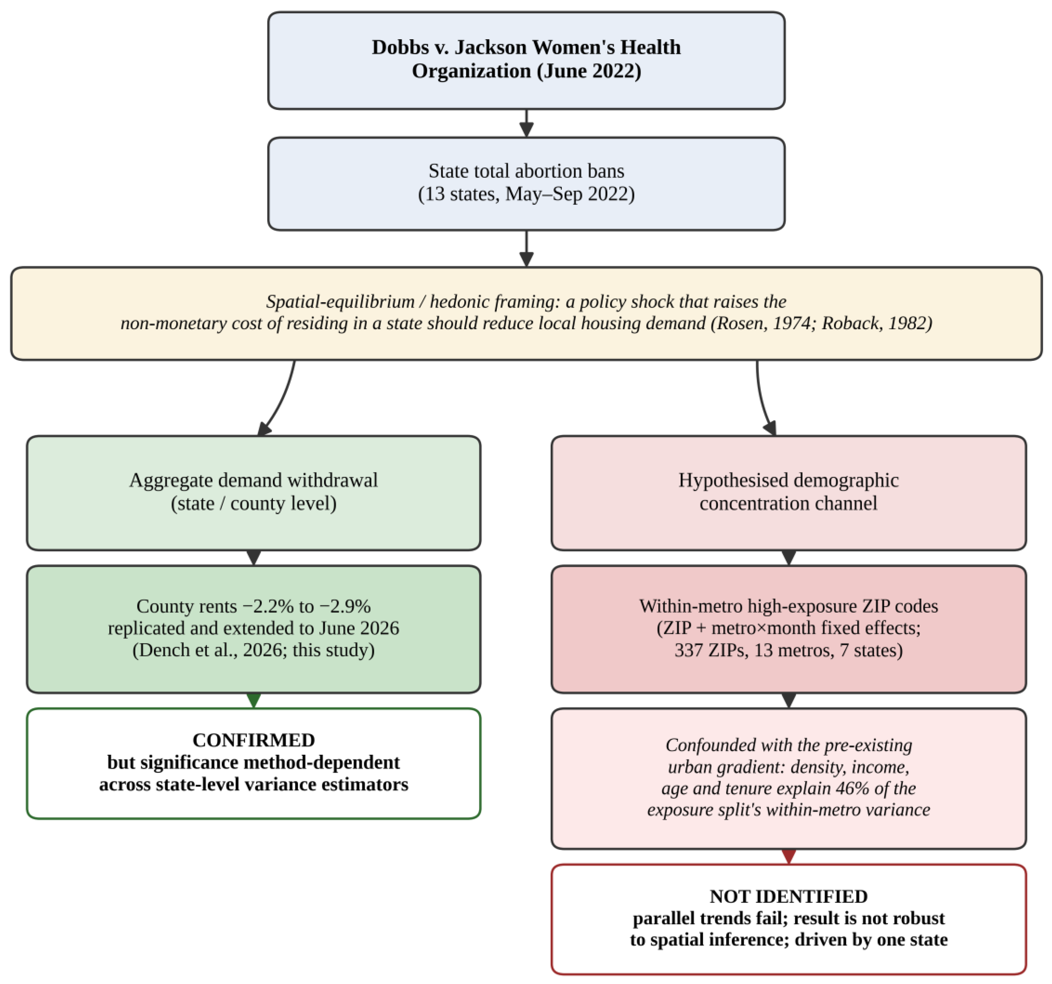
Figure 2.
High- and low-exposure ZIP codes in the four largest ban-state metropolitan areas, located at ZIP Code Tabulation Area internal points. Grid lines mark 0.25° cells, the block size used for spatially blocked permutation. Moran’s I is computed within each metropolitan area on inverse-distance weights. Authors’ own elaboration based on ACS 2016–2020 and the 2020 Census Gazetteer.
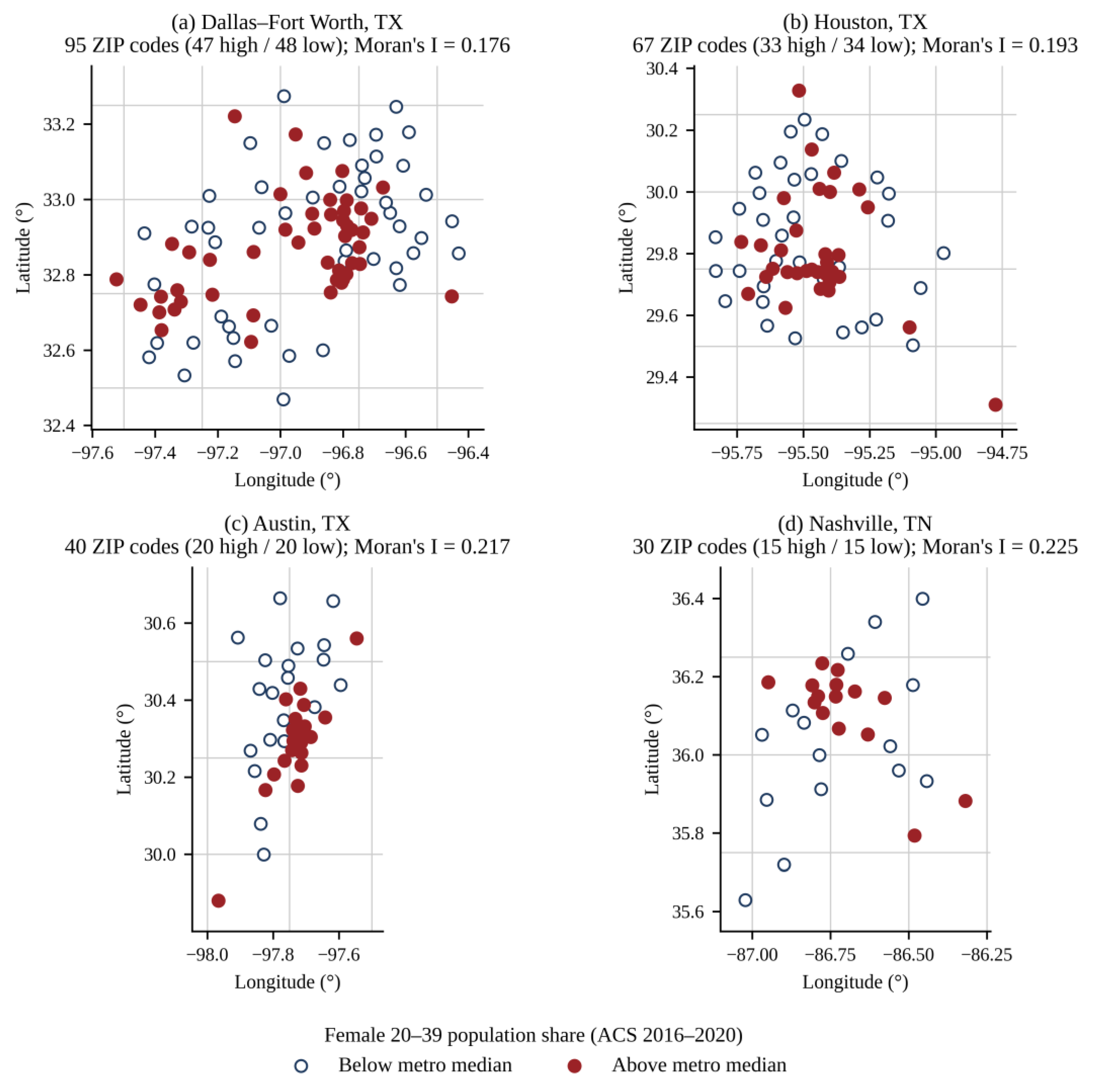
Figure 3.
Within-metropolitan exposure gap in ban-state metropolitan areas on the per-state event clock: event-study coefficients at selected event times relative to month −1. Filled markers denote p < 0.05 with standard errors clustered by state. Authors’ own elaboration.
Figure 3.
Within-metropolitan exposure gap in ban-state metropolitan areas on the per-state event clock: event-study coefficients at selected event times relative to month −1. Filled markers denote p < 0.05 with standard errors clustered by state. Authors’ own elaboration.
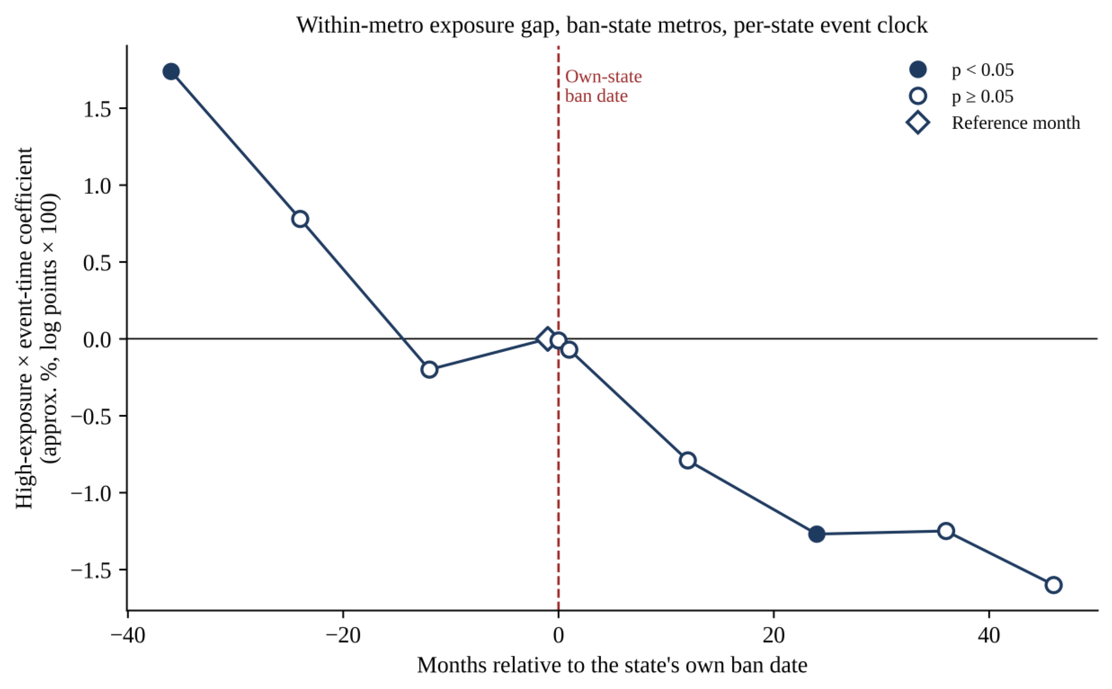
Figure 4.
Pre- and post-ban exposure-gap slopes under two estimation windows, with 95% confidence intervals (state clusters, t with six degrees of freedom). Authors’ own elaboration.
Figure 4.
Pre- and post-ban exposure-gap slopes under two estimation windows, with 95% confidence intervals (state clusters, t with six degrees of freedom). Authors’ own elaboration.
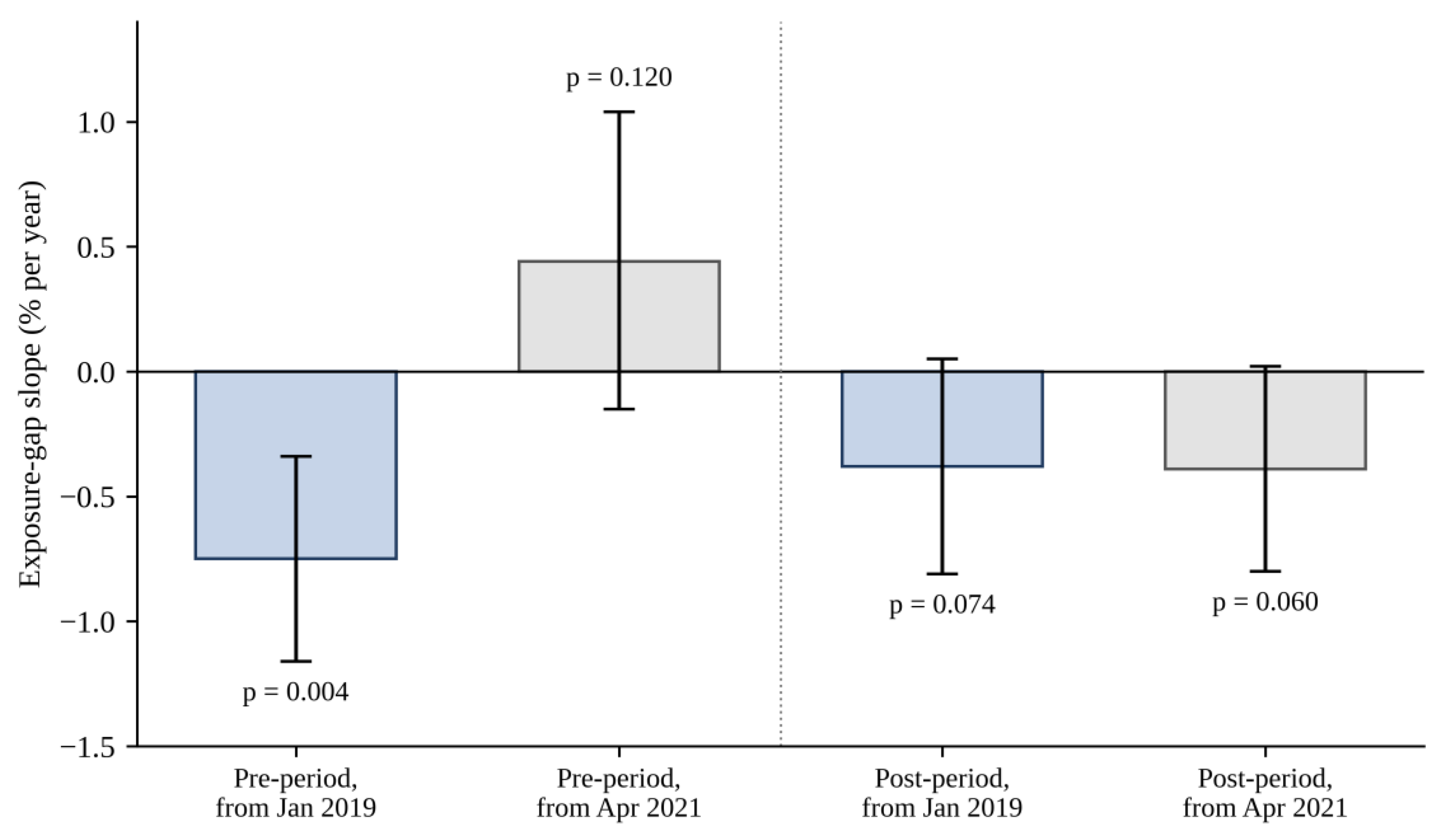
Figure 5.
Significance of the within-metropolitan differential under ten inference procedures. Authors’ own elaboration.
Figure 5.
Significance of the within-metropolitan differential under ten inference procedures. Authors’ own elaboration.
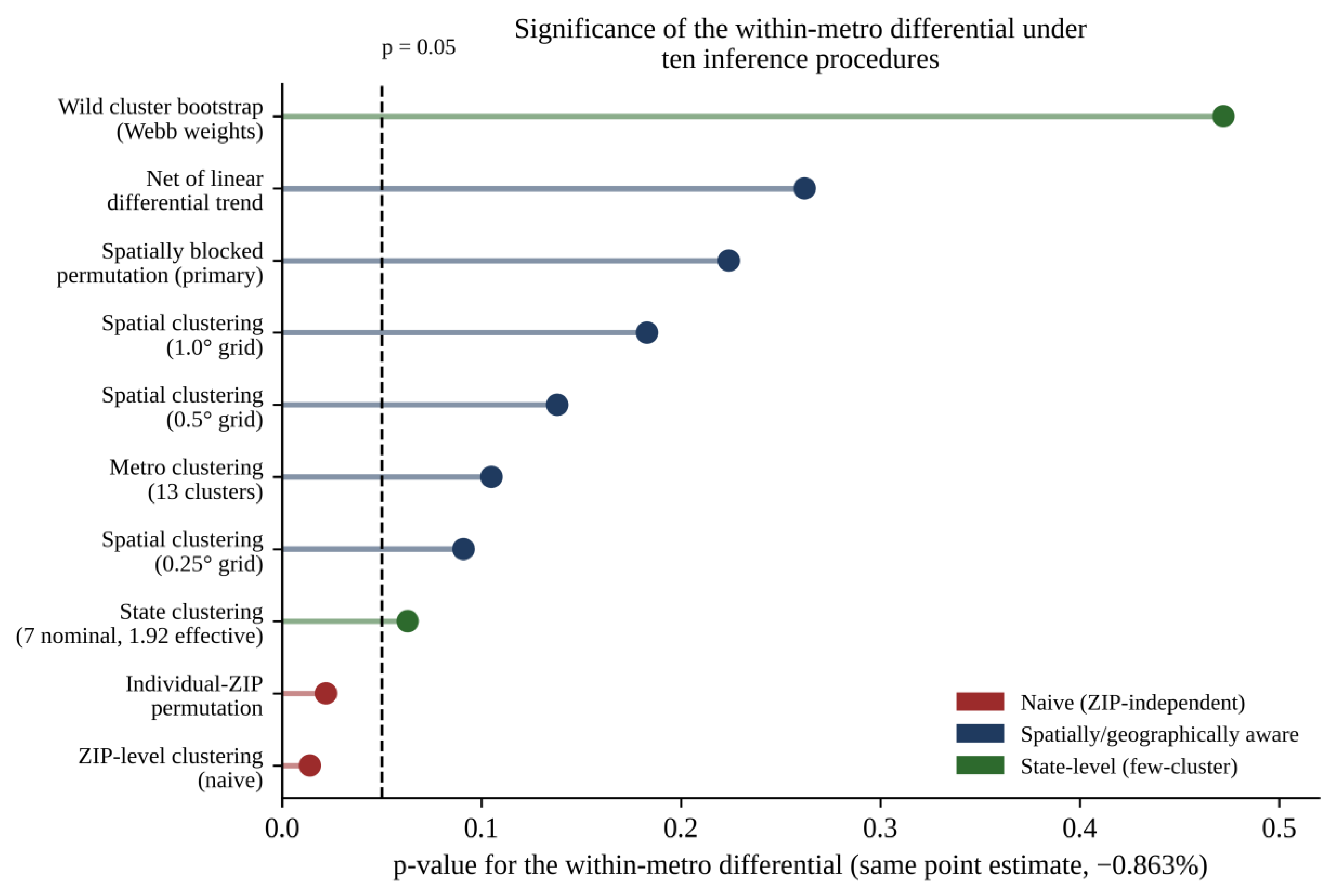
Figure 6.
Triple difference with 95% confidence intervals: (a) additional movement in the ban-metropolitan exposure gap relative to protecting-state metropolitan areas (β₂); (b) difference between ban and intermediate tiers (β₂ − β₃). Dotted lines mark ±1%. Authors’ own elaboration.
Figure 6.
Triple difference with 95% confidence intervals: (a) additional movement in the ban-metropolitan exposure gap relative to protecting-state metropolitan areas (β₂); (b) difference between ban and intermediate tiers (β₂ − β₃). Dotted lines mark ±1%. Authors’ own elaboration.
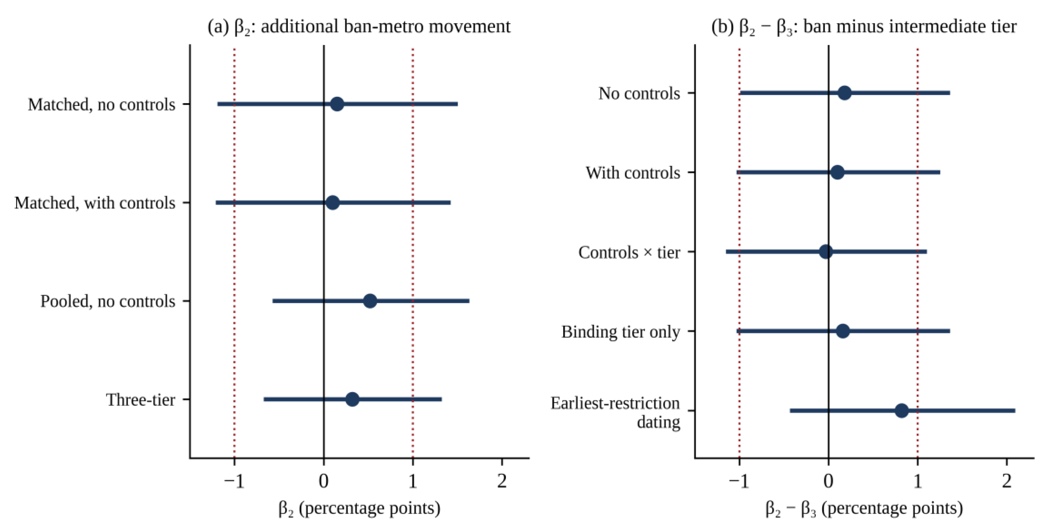

Table 1.
Sample construction and geographic coverage.
| Stage | ZIP codes |
| Zillow ZORI ZIP codes, raw | 8,477 |
| Matched to ACS exposure measure | 8,449 |
| ≥80% pre-treatment coverage (Jan 2019–May 2022) | 2,214 |
| In classified states and metropolitan areas | 2,210 |
| Final analytical sample | 1,651 |
| — Ban tier (13 metros, 7 states) | 337 |
| — Intermediate tier (24 metros, 9 states) | 597 |
| — Protecting tier (23 metros, 12 states) | 717 |
| Pooled ban and protecting (triple-difference base) | 1,054 |
| Matched triple-difference sample | 662 (337 ban, 325 protecting) |
Table 1: Authors’ own elaboration based on Zillow ZORI and ACS 2016–2020.
Table 2.
Within-metropolitan exposure differential: point estimates and inference.
| Specification | Estimate (%) | 95% CI | MDE (80%) | p |
| Median split, no covariate adjustment | −0.86 | [−1.78, 0.07] | 1.28 | 0.063 |
| Median split, covariates × Post | −0.84 | [−2.06, 0.40] | 1.71 | 0.148 |
| Continuous, per 10pp of female share | −1.72 | [−2.53, −0.91] | 1.14 | 0.002 |
| Continuous, covariates × Post | −1.48 | [−2.20, −0.75] | 1.02 | 0.003 |
| Strict nine-metro sample | −1.01 | [−1.86, −0.16] | 1.17 | 0.028 |
| Equal-metropolitan weighting | −0.011 | [−1.22, 1.22] | — | 0.983 |
| Population weighting within metropolitan area | +0.160 | [−0.85, 1.18] | — | 0.713 |
| Resident-population weighting | −0.665 | [−1.49, 0.16] | — | 0.097 |
| Excluding Texas (99 ZIPs) | +0.04 | [−2.17, +2.30] | — | 0.967 |
| Median split, spatially blocked permutation (primary inference) | −0.86 | — | — | 0.224 |
Table 2: Authors’ own elaboration. MDE is the minimum detectable effect at 80% power. Standard errors clustered by state unless stated.
Table 3.
Specificity test: placebo discrimination (Panel A) and sex-composition estimates (Panel B).
Table 3.
Specificity test: placebo discrimination (Panel A) and sex-composition estimates (Panel B).
| Panel A: Candidate exposure measures and classification agreement | |||||
| Measure | Correlation with treatment | Same classification | Verdict | ||
| Male 20–39 share | 0.741 | 88.7% | Low power, uninformative placebo | ||
| Female 50–69 share | −0.626 | 30.6% | Sign-flipped proxy, not a null test | ||
| Female minus male, 20–39 | 0.008 | 46.6% | Discriminating | ||
| Female-to-male ratio, 20–39 | 0.024 | 45.4% | Discriminating | ||
| Panel B: Sex-composition specificity estimates (H2) | |||||
| Measure | Estimate (%) | 95% CI | MDE (80%) | Verdict | |
| Female − male gap, median split | +0.07 | [−0.32, +0.46] | 0.54 | Informative null | |
| Female − male gap, per SD | +0.37 | [−0.12, +0.86] | 0.67 | Informative null | |
| Female-to-male ratio, median split | +0.08 | [−0.38, +0.54] | 0.63 | Informative null | |
| Female-to-male ratio, per SD | +0.26 | [−0.07, +0.58] | 0.44 | Informative null | |
Table 3: Authors’ own elaboration based on ACS 2016–2020 and Zillow ZORI.
Table 4.
Replication and one-year extension of Dench et al. (2026).
| Outcome / window | This study | Dench et al. (2026) published |
| Rents, Jul 2022–Jun 2025 | −2.20% | −2.2% |
| Rents, final year (Jul 2024–Jun 2025) | −3.96% | −4.0% |
| Home values, Jul 2022–Jun 2025 | −1.77% | −1.8% (reported n.s.) |
| Extension: rents, Jul 2022–Jun 2026 | −2.87% | n/a (extension) |
| Extension: rents, newest year (Jul 2025–Jun 2026) | −5.02% | n/a (extension) |
| Extension: home values, Jul 2022–Jun 2026 | −2.32% | n/a (extension) |
| Rent county sample (ban / protecting) | 79 / 175 | 76 / 172 |
| Home-value county sample (ban / protecting) | 647 / 630 | 647 / 630 |
Table 4: Authors’ own elaboration based on Zillow ZORI and ZHVI; published figures from Dench et al. (2026).
Disclaimer/Publisher’s Note: The statements, opinions and data contained in all publications are solely those of the individual author(s) and contributor(s) and not of MDPI and/or the editor(s). MDPI and/or the editor(s) disclaim responsibility for any injury to people or property resulting from any ideas, methods, instructions or products referred to in the content. |
© 2026 by the authors. Licensee MDPI, Basel, Switzerland. This article is an open access article distributed under the terms and conditions of the Creative Commons Attribution (CC BY) license.
Copyright: This open access article is published under a Creative Commons CC BY 4.0 license, which permit the free download, distribution, and reuse, provided that the author and preprint are cited in any reuse.