

Submitted:
05 October 2026
Posted:
09 October 2026
You are already at the latest version
Abstract
In many contemporary studies on solar activity, time is typically treated as a single variable or as a linear variable over a given timescale. In traditional Chinese culture, time is represented by two ordinal categorical labels—Heavenly Stems and Earthly Branches—across four timescales. In recent studies, these two categorical variables were transformed into two cosine waves and significant correlations were found between these waves and the yearly variations in tropical cyclones and sunspot numbers. This study followed the methods of previous studies and provided explicit mathematical expressions. The objective of this study was to investigate the possible relationship between time represented by two cosine waves derived from the Ganzhi calendar and the spatial attributes of solar activity. Results showed that, on the yearly timescale, significant correlations were found between the two cosine waves and solar activity in the northern and southern hemispheres of the Sun, and three distinct patterns were identified. Based on these results, a linear formula for solar activity was proposed, from which estimates for the sunspot cycle and the solar magnetic cycle can be derived. In conclusion, treating time as two cosine waves may be useful for extracting spatial as well as temporal information from solar activity.
Keywords:
solar activity
; solar cycle
; sunspot number
; Tiangan–Dizhi
; north–south asymmetry
; butterfly diagram
; solar polar magnetic field strength
; Ganzhi calendar
1. Introduction
Solar activity exerts a profound impact on various aspects of human existence [1,2,3], yet accurately predicting it remains a considerable challenge [4]. Sunspots appear as dark regions on the solar surface, with the sunspot number (SN) serving as the primary indicator of solar activity. Currently, various methods are employed to forecast the maximum sunspot number or the amplitude of upcoming solar cycles [5,6]. Among the 12 methods reviewed in [7], the polar field approach was shown to be the most accurate for predicting the maximum of Solar Cycle 24.
In the conventional view, time is regarded as a one-dimensional phenomenon; accordingly, in most previous studies, whether pertaining to solar activity or extending across various disciplines, time has generally been treated as a single variable or a straight line. However, in the traditional Chinese Stems-and-Branches time-reckoning system (Tiangan–Dizhi or Ganzhi calendar), time is denoted using two categorical variables simultaneously: one from the 10 Heavenly Stems (Tiangan, T) and the other from the 12 Earthly Branches (Dizhi, D).
For example, on the yearly timescale, the year 2025 is denoted as Yi-Si, where "Yi" is the 2nd element of the 10 Stems and "Si" is the 6th element of the 12 Branches. This coding scheme applies uniformly to the hourly, daily, monthly, and yearly timescales.
Two recent studies employing the Ganzhi calendar have provided valuable insights into the longstanding challenge of predicting sunspot activity. In the first study, because tropical cyclone frequencies exhibit periodic variations on the daily, monthly, and yearly timescales, and because the T and D variables also exist on the three scales, the two variables were quantified, drawing on ancient assertions, as two cosine waves (with T = 1−cos(1.2θ) and D = 1−cosθ), and the possible relationships of these waves with tropical cyclone frequencies on each scale were then examined. The results showed that the difference between the two cosine waves on the yearly timescale correlated significantly with the 6-hourly frequencies of tropical cyclones over the western North Pacific from 1956 to 2016 (p < 0.05) [8]; this correlation was later also found on the daily timescale [9] (p. 216). These findings demonstrated the feasibility of transforming the two categorical variables into the two cosine waves. In the second study, the SN (which also varies on daily, monthly, and yearly timescales) from 1749 to 2018 was found to correlate significantly with the two cosine waves in an alternating manner on the yearly timescale: specifically, SN correlated significantly with the D wave during 1864–1923, then with the T wave during 1924–1983, and again with the D wave during 1984–2018 [9] (pp. 221–241). This alternating pattern was also observed for the sunspot group number (SGN) (see Appendix A).
The previous study [9] (pp. 221–241) examined the relationship between the temporal attributes of sunspot number and the cosine waves. This companion paper aims to further investigate, across the three timescales (daily, monthly, and yearly), the possible relationship between the spatial attributes of solar activity and the T and D cosine waves.
The null hypothesis was that there was no correlation between the cosine waves and the spatial attributes of solar activity on any of the three timescales.
2. Materials and Methods
2.1. Materials
The analysis focused on spatial attributes of solar activity, including north–south sunspot numbers (N–S SN), the butterfly diagram, and solar polar magnetic field strength.
N–S SN: Sunspot numbers recorded separately for the northern and southern (N–S) hemispheres of the Sun. The monthly mean N–S SN data (June 1944–May 2018, N = 888) were obtained from the Kanzelhöhe Solar Observatory (KSO) (http://cesar.kso.ac.at/synoptic/num_years.php).
Butterfly diagram: A two-dimensional representation of average sunspot coverage as a function of time (horizontal axis) and heliospheric latitude (vertical axis), resembling butterfly wings. The data (Nov. 5, 1825–Jan. 4, 2016, N = 52,804) were from VizieR (http://vizier.cfa.harvard.edu/viz-bin/VizieR?-source=J/A+A/599/A131).
Solar polar magnetic field strength: Data (May 31, 1976–May 21, 2018, N = 1,534) were taken from the Wilcox Solar Observatory (WSO) Polar Field Observations (see the item “Solar Polar Field Strength since 1976” at http://wso.stanford.edu/#MeanField).
2.2. Methods
The T–D calendar has been used for thousands of years and remains in use today. A T–D hour equals two Gregorian hours (e.g., 21:00–23:00 constitutes one T–D hour); a T–D day has the same duration as a Gregorian day but begins at 23:00 on the previous day and lasts 24 hours; a T–D month typically starts on a day between the 4th and 7th days of a Gregorian month and ends on a day between the 4th and 7th days of the following month; and a T–D year generally runs from Feb. 4 of one year to Feb. 3 of the next year.
In the T–D calendar, one T and one D are used sequentially in pairs to record time. These pairs are applied to the four timescales and cycle through 60 pairs (also known as the sexagenary cycle): Shi (T–D hour), Ri (T–D day), Yue (T–D month), and Sui (T–D year).
The following paragraphs describe how the ancient assertions described above were translated into modern mathematical formulas.
The ancient Chinese evenly allocated the T and D around the 360° circumference of the celestial sphere, and they also believed that the T (Yang) and D (Yin) components each progressed through the stages of birth, growth, prime, decline, and death. Based on these assertions, the two groups of discrete variables (10 and 12 components) were quantified as two continuous variables, i.e., two cosine waves [8]. In this way, over a single T–D year, the T on the yearly timescale (yT) was expressed as formula (1), and the D on the yearly timescale (yD) was expressed as formula (2):
In a sexagenary cycle of 60 years (equivalent to 360°·60, or 21,600°), T cycles six times (10·6·360°), and D cycles five times (12·5·360°). Thus, the yearly T (yT) cosine wave over a sexagenary cycle is given by formula (3), and the yearly D (yD) by formula (4):
The monthly T (mT) over the same cycle is given by formula (5), and the monthly D (mD) by formula (6):
The daily T (dT) is given by formula (7), and the daily D (dD) by formula (8):
Additionally, in ancient Chinese philosophy, the weight of a specific T or D component on each of the four timescales is its frequency: the more frequent a given component is, the greater its weight (effect or influence).
For example, consider two time points. At the first time point, the four timescales are labeled as "T1D1 T2D2 T3D3 T4D4", so T1 occurs once. At the second time point, the labels are "T1D1 T1D3 T1D5 T1D7", so T1 occurs four times. In this case, the ancient Chinese believed that T1 at the second time point exerted a greater effect than at the first. This belief implies that the frequency of a given component serves as its weight on each timescale, thereby justifying the averaging of the waves across the four timescales. Following this reasoning, the waves from the four timescales were averaged with equal weights, yielding the following averaged waves.
First, the average of the monthly and yearly T (myT) over a sexagenary cycle of 60 T–D years is given by formula (9), where mT(θ) and yT(θ) are defined in formulas (5) and (3), respectively. The average of the monthly and yearly D (myD) over a sexagenary cycle is given by formula (10), where mD(θ) and yD(θ) are defined in formulas (6) and (4), respectively.
Second, the average of daily and monthly T (dmT) over a sexagenary cycle of 60 T–D years is given by formula (11), where dT(θ) and mT(θ) are defined in formulas (7) and (5), respectively. The average of daily and monthly D (dmD) is given by formula (12), where dD(θ) and mD(θ) are defined in formulas (8) and (6), respectively.
Third, the average of daily, monthly, and yearly T waves (dmyT) over a sexagenary cycle of 60 T–D years is given by formula (13), and the corresponding average for D (dmyD) is given by formula (14).
Because hourly solar data were not available, hourly waves and the averaged waves involving them were not defined in the present analysis.
In this way, the averaged waves can also serve as a tool for investigating possible relationships between them and variations in solar activity.
3. Results
3.1. Correlation Between KSO N–S Monthly SN Data and T/D Cosine Waves
The earlier study focusing on temporal attributes of SN found that SN correlated significantly with the yearly T wave in the sexagenary cycle from 1924 to 1984, whereas SN correlated significantly with the yearly D wave—but not with the yearly T wave—in the 1984–2018 interval of the following sexagenary cycle [9] (pp. 231–237). Therefore, in analyzing the spatial attributes of the KSO N–S SN, the data were divided into two parts in early 1984 (Figure 1): Part 1, spanning June 1944 to Jan. 1984, was dominated by the yearly T cosine wave; Part 2, spanning Feb. 1984 to May 2018, was dominated by the yearly D cosine wave.
For the entire period, SN exhibited significant correlations with yT (r = 0.44, p < 0.0001), myT (r = 0.32, p < 0.0001), and the difference between yT and yD (yT − yD) (r = 0.19, p < 0.0001), but not with yD, myD, mT, or mD (Table 1).
In Part 1 (June 1944–Jan. 1984), northern sunspot numbers (nSN) were significantly positively correlated with yT (r = 0.77, p < 0.0001) (Figure 1, left panel, red curves), yD (r = 0.35, p < 0.0001), myT (r = 0.56, p < 0.0001), and myD (r = 0.21, p < 0.0001), but not with mT or mD; in contrast, southern sunspot numbers (sSN) were significantly negatively correlated with yT (r = −0.54, p < 0.0001), yD (r = −0.47, p < 0.0001), myT (r = −0.38, p < 0.0001), and myD (r = −0.34, p < 0.0001), but not with mT or mD.
In Part 2 (Feb. 1984–May 2018), nSN were significantly positively correlated with yT (r = 0.16, p < 0.0001) and myT (r = 0.11, p < 0.05), and significantly negatively correlated with yD (r = −0.72, p < 0.0001) and myD (r = −0.51, p < 0.0001), but not with mT or mD; meanwhile, sSN correlated significantly with yD (r = 0.71, p < 0.0001) (Figure 1, right panel, black curves) and myD (r = 0.48, p < 0.0001), but not with yT, myT, mT, or mD.
Additionally, over the entire period, the difference between nSN and sSN (nSN − sSN) correlated significantly with the difference between yT and yD (yT − yD) (r = 0.19, p < 0.0001) (Figure 1, bottom panel, blue curves).
3.2. Correlation Between SN Latitudes and T/D Waves in Degrees
The latitude distribution of sunspots in the butterfly diagram was analyzed, and it was found that the θ values corresponding to yT and yD (in degrees, rather than their cosine-wave values) correlated significantly with heliographic latitudes.
First, over the entire time range, no correlation was found between the latitudes and either cosine wave (yT or yD) on the yearly timescale. Nevertheless, yT and yD can also be expressed in degrees (obtained at Step 3 of the transformation from the Gregorian calendar to the Chinese calendar; see Table 1 of [8]), an approach that was more appropriate for the correlation analysis. Because the degree values for yT and yD both range from 0 to 360, for positive correlations the range was inverted (from 360 to 0) (for yT in degrees, see the oblique dashed lines at the top of Figure 2; for yD, see those at the bottom). The values in degrees were shown on the rightmost part of Figure 2.
Over the entire time range, the northern latitudes correlated significantly with the θ values for yT (r = 0.15, p < 0.0001) and yD (r = 0.02, p < 0.0001); the southern latitudes correlated significantly with the θ values for yT (r = 0.11, p < 0.0001) and yD (r = 0.04, p < 0.0001).
The cycle-by-cycle analysis was performed between the latitudes and the θ values for yT and yD. Because the northern latitudes were mainly correlated with the θ values for yT, and the southern latitudes with those for yD, only the correlation coefficients and significance levels for the northern latitudes with yT θ values (upper part of Figure 2) and for the southern latitudes with yD θ values (lower part of Figure 2) were shown.
From the red lines at the top and black lines at the bottom, three distinct patterns emerged. First, the yT-dominant pattern, in which the θ values for yT were significantly correlated with the latitudes in both hemispheres (Feb. 1828–Jan. 1864, Feb. 1924–Jan. 1984); second, the yD-dominant pattern, in which the θ values for yD were significantly correlated with the latitudes (Feb. 1876–Jan. 1904, Feb. 2004–Jan. 2016); third, the mixed pattern, in which the θ values for yT and yD were both significantly correlated with the latitudes (Nov. 1825–Jan. 1828, Feb. 1904–Jan. 1924, and Feb. 1984–Jan. 2004), or in which the θ values for yT and yD were not significantly correlated with the latitudes (Feb. 1864–Jan. 1876).
3.3. Correlation of Poloidal Magnetic Values and T/D Waves
The data (both raw and filtered at 20 Hz) were averaged over 10-day intervals. Therefore, correlation analyses were conducted only for the monthly (mT, mD), yearly (yT, yD), and their averaged waves (myT, myD). These analyses were performed within 10-year intervals of yT (Table 2) and 12-year intervals of yD (Table 3). Correlations between the northern raw data and yT (Figure 3, upper part) and between the southern raw data and yD (Figure 3, lower part) were also shown. Because the southern data were predominantly negative, negated D waves (i.e., −yD, −mD, and −myD) were employed in the present analysis.
Over the entire data, the raw northern data were significantly positively correlated with yT (r = 0.17, p < 0.0001) and myT (r = 0.12, p < 0.001), but not with −yD, mT, −mD, or −myD. In contrast, the raw southern data showed no significant positive correlation with any of the waves. The results for the 20-Hz-filtered northern data were very similar to those for the raw data.
It can be easily seen that the zero-crossing points (defined as the points nearest to zero) of the filtered data divide the data into several ranges. This raises an interesting question: within each range, how do the waves differ in their correlations with the data? Correlation analyses were therefore performed between these waves and the data—including the northern data (Figure 4) and the southern data (Figure 5)—within the six ranges defined by the zero-crossing points of the filtered data (Table 4).
4. Discussion
In this study, correlation analyses were performed between the solar activity data and various waves derived from the Chinese Ganzhi calendar.
First, a key finding is that solar activity was significantly correlated with the yT and −yD waves and these correlations exhibited three distinct patterns, thereby rejecting the working hypothesis. In the yT-dominant pattern, the yT cosine wave was significantly correlated with northern solar activity (see the red correlation coefficients in the upper panels of Figure 1, Figure 2, Figure 3, Figure 4 and Figure 5). In the −yD-dominant pattern, the −yD cosine wave was significantly correlated with southern solar activity (see the black correlation coefficients in the lower panels of Figure 1, Figure 2, Figure 3, Figure 4 and Figure 5). In the mixed pattern, either both yT and −yD were significantly correlated with solar activity (for example, Range 5 in the North and Range 1 in the South in Table 4), or neither was correlated with solar activity (Range 1 in the North and Ranges 5 and 6 in the South in Table 4). These three patterns were also observed previously in the SN [9] (p. 233) and SGN data (see Figure A1 in Appendix A).
Consequently, in a phenomenological sense, a linear combination of the yT and −yD cosine waves can correlate significantly with aforementioned solar activity:
In the formula (15), S represents the solar activity, and yT(θ) and yD(θ) were defined as in (3) and (4), respectively.
This formulation may reasonably describe the aforementioned solar activity as follows: when α₁ is very large and α₂ is very small, the yT-dominant pattern emerges (mostly in the northern hemisphere); when α₁ is very small and α₂ is very large, the −yD-dominant pattern emerges (mostly in the southern hemisphere); and when α₁ and α₂ are nearly equal (both very small or both very large), the mixed pattern appears. Thus, when combined with additional parameters, formula (15) might well describe and fit most solar activity. Furthermore, the difference wave yT − yD, which can be seen as a special example when α₁ = α₂, was found to be significantly correlated with the difference in SN between the northern and southern hemispheres of the Sun (Figure 1) as well as with tropical cyclone frequencies [9] (p. 217). In addition, based on formula (15), the period of the solar cycle may be obtained in units of time or degrees. The yT cycle is 10 T–D years and the yD cycle is 12 T–D years; therefore, the solar cycle would be their mean, i.e., 11 T–D years (approximately equal to 11 Gregorian years). Expressed in degrees, one T–D year equals 360°, so 60 T–D years equal 21,600°. Thus, the 10 T–D year cycle is 3,600° for T and the 12 T–D year cycle is 4,320° for D, so the solar cycle on the yearly timescale would be 3,960°. As for the polar field cycle on the yearly timescale, it would be the sum of the T and D cycles, corresponding to 22 T–D years (approximately 22 Gregorian years), or 7920°.
Second, in most previous studies, time has been treated as a single monotonically increasing index variable—effectively a linear coordinate on the timescale. While this coordinate serves as a useful numerical feature, it captures only the sequential ordering of events and inevitably discards the multi-dimensional cyclic phase structures that are often intrinsic to natural phenomena. Our results demonstrate that this neglect is not merely a theoretical concern. The three alternating patterns we observed—yT-dominant, −yD-dominant, and mixed—were detectable only when time was decomposed into two independent cyclic components. The traditional Chinese Stems-and-Branches system, which encodes time as two simultaneous categorical cycles (T and D), provided the conceptual basis for this decomposition. By transforming these two categories into cosine waves, we effectively replaced a one-dimensional monotonic variable with a two-dimensional circular representation. This transformation enabled the identification of periodic spatial variations that the single-coordinate approach inherently fails to detect. Notably, it yielded a simple linear formulation, namely formula (15), with remarkable parsimony. Since the significant correlations between the aforementioned solar activity and the yT and −yD waves can be described reasonably by formula (15), solar activity appears to be, at least in part, a linear phenomenon.
Third, regarding the N–S asymmetries, Temmer et al. previously reported that approximately 60% of the monthly N–S asymmetries were significant [10]. In the present study, correlation results between the yearly waves (yT and −yD) and the data (the KSO N–S monthly sunspot number data and polar magnetic field data) indicated that formula (15), with additional parameters, could reasonably describe such asymmetries.
Fourth, the correlation between sunspot latitudes and the θ values can be used to predict the spatial attributes of sunspots. In Figure 2, there are 18 pairs of butterfly wings, with the right wing in the upper part (northern hemisphere) and the left wing in the lower part (southern hemisphere); the heads are on the left and the tails on the right. At the top of Figure 2 are the red lines representing θ for yT, and at the bottom are the black lines representing θ for yD. The slopes of the red lines are notably steeper than those of the black lines. Interestingly, for the two wings (one in each hemisphere) that correlate significantly with the red lines, the angles between the anterior (left) parts of the wings are relatively large (close to 180°); however, for the two wings that correlate significantly with the black lines, the corresponding angles are narrower (close to 160°). It is also observed that when a pair of butterfly wings correlates significantly with the θ values, its range nearly overlaps with that of the corresponding cosine wave. For example, the rightmost (18th) pair of butterfly wings correlates significantly with θ for yD, and its range overlaps more with yD wave than with yT wave. Overall, these results may help predict the spatial attributes of sunspots in future work.
Fifth, currently, only data covering the three timescales (daily, monthly, and yearly) are used. In this study, significant correlations were discovered mostly on the yearly timescale, yet significant correlations also existed on the monthly timescale (Table 4). While daily data on solar activity were absent in this study, it was found in the previous study [9] (p. 216) that tropical cyclone activity on the daily timescale was significantly correlated with the daily cosine waves. Based on these results, it is reasonable to assume that solar activity on the three timescales should be significantly correlated with the waves on the corresponding timescales. This might also hold true for tropical cyclones, as the activities on the yearly [8] and daily [9] (p. 216) timescales were significantly correlated with the waves on the corresponding timescales in the previous studies.
Sixth, the Chinese time system could also be used to analyze solar activity on longer timescales. SN is known to exhibit such variations. For example, on the multi-decadal to centennial scale, the Gleissberg cycle [11] has a period of approximately 90 years, with a period varying between 60 and 120 years [12]. On the centennial scale, the 210-year Suess cycle has been identified [13]. On the millennial scale, SN has been reconstructed over the last 11,000 years [14,15], revealing a 2,400-year Hallstatt cycle [16]. In fact, longer-period T and D waves also exist in the Chinese time system, and these long-period cosine waves may prove useful for analyzing long-term solar activity. The Chinese time system traditionally encompasses four timescales, yet a recent study [17] expanded it to a seven-timescale system, and another study [9] (pp. 160–163) extended it to a system with theoretically infinite timescales, which spans periods from seconds to tens of thousands of years and beyond. Such a multi-timescale framework might be useful for addressing variations across multiple timescales in solar activity and related phenomena.
Seventh, the 60-year cycle is an important cycle in many natural phenomena and has been discussed by some researchers. Weng and Zhang analyzed time series of various natural disasters—including earthquakes, droughts, floods, and tropical cyclones—and found that the 60-year sexagenary cycle was a fundamental cycle [18]. This 60-year cycle has also been identified in modern analyses [19].
In the Chinese Ganzhi calendar, the start and end of these 60-year cycles are set and well defined. For example, the nearest cycles are Feb. 5, 1804–Feb. 3, 1864, Feb. 4, 1864–Feb. 4, 1924, Feb. 5, 1924–Feb. 3, 1984, and Feb. 4, 1984–Feb. 3, 2044. However, solar activity did not show a good fit with these ending time points except on Feb. 4, 1924, when the SN and SGN dropped to zero, and both yT and yD (in the previous studies, the yD took the positive values) also reached zero; see [9], p. 232); the reason is currently unknown, and further research is needed in the future.
In the Chinese Ganzhi calendar, the start and end of these 60-year cycles are set and well defined. For example, the most recent cycles are Feb. 5, 1804–Feb. 3, 1864, Feb. 4, 1864–Feb. 4, 1924, Feb. 5, 1924–Feb. 3, 1984, and Feb. 4, 1984–Feb. 3, 2044. However, solar activity did not show a good fit with these end points except on Feb. 4, 1924, when the SN dropped to zero, and both yT and yD (in previous studies, yD was defined as positive) also reached zero (see [9], p. 232); the reason is currently unknown, and further research is needed.
Finally, our method, derived from the Yin-Yang philosophy, is novel and differs considerably from previous approaches that relied on cycle statistics [20,21], geomagnetic precursors [22,23,24], polar field measurements [25,26], dynamo models [27,28], machine learning [29], and other approaches. In the Yin-Yang philosophy, the two factors (Yang/T and Yin/D) are thought to be related to all phenomena in the universe. Our studies on solar activity and tropical cyclones provide some support for this ancient philosophical framework. We acknowledge, however, that a detailed discussion of the underlying physical mechanism lies beyond the scope of this work, as it would require specialized expertise in solar physics.
5. Conclusions
Overall, the dual cosine waves derived from the ancient Chinese calendar proved valuable for uncovering spatial patterns in solar activity. Given that this approach has provided insights into solar activity as well as tropical cyclone activity, it may hold promise for applications in other fields.
Data Availability Statement
The original data presented in the study are openly available (for details, see “2.1. Materials”).
Acknowledgments
The author gratefully acknowledges the use of data from the Kanzelhöhe Solar Observatory (KSO), the VizieR catalogue service, the Wilcox Solar Observatory (WSO), and the Sunspot Index and Long-term Solar Observations (SILSO) at the Royal Observatory of Belgium.
Conflicts of Interest
The author declares no conflict of interest.
Abbreviations
The following abbreviations are used in this manuscript:
| SN | sunspot number |
| T | Tiangan |
| D | Dizhi |
| T–D | Tiangan–Dizhi |
| SGN | sunspot group number |
| N–S | northern and southern |
| KSO | Kanzelhöhe Solar Observatory |
| WSO | Wilcox Solar Observatory |
| yT | T on the yearly timescale, or the yearly T |
| yD | the yearly D |
| mT | monthly T |
| mD | monthly D |
| dT | daily T |
| dD | daily D |
| myT | average of the monthly and yearly T waves |
| myD | average of the monthly and yearly D waves |
| dmT | average of daily and monthly T waves |
| dmD | average of daily and monthly D waves |
| dmyT | average of daily, monthly, and yearly T waves |
| dmyD | average of daily, monthly, and yearly D waves |
| nSN | northern sunspot numbers |
| sSN | southern sunspot numbers |
Appendix A. Correlation Between SGN and T/D Waves
1. Data
The annual sunspot group numbers (SGN) were obtained from Svalgaard 2016 (S16) (1610–2015, N = 406) [30], Usoskin 2016 (U16) (1749–1995, N = 247) [31], and Cliver 2016 (C16) (1841–1976, N = 136) [32].
2. Analysis
In summary, the annual sunspot group numbers (SGN) from Svalgaard 2016 (S16), Usoskin 2016 (U16), and Cliver 2016 (C16) exhibited significant correlations with the yearly T variable (for S16, r = 0.25, p < 0.0001; U16, r = 0.39, p < 0.0001; C16, r = 0.38, p < 0.0001), but not with the yearly D variable (Table A1, row 1 to row 6).

Table A1.
Correlation between the SGN data and the waves.
| No. | Data | Type | y | m | d | my | dmy |
|---|---|---|---|---|---|---|---|
| 1 | S16 yearly | T | 0.2484*** | NA | NA | NA | NA |
| D | NS | NA | NA | NA | NA | ||
| 2 | U16 yearly | T | 0.3885*** | NA | NA | NA | NA |
| D | NS | NA | NA | NA | NA | ||
| 3 | C16 yearly | T | 0.3823*** | NA | NA | NA | NA |
| D | NS | NA | NA | NA | NA | ||
| 4 | U16 monthly | T | 0.3904*** | NS | NA | 0.2707*** | NA |
| D | 0.084*** | NS | NA | 0.0606*** | NA | ||
| 5 | C16 monthly | T | 0.3635*** | NS | NA | 0.2564*** | NA |
| D | 0.0878*** | NS | NA | 0.0721*** | NA | ||
| 6 | U16 daily | T | 0.3614*** | -0.0085* | NS | 0.2499*** | 0.2046*** |
| D | 0.0901*** | NS | NS | 0.0669*** | 0.0554*** | ||
| 7 | C16 daily | T | 0.3256*** | NS | NS | 0.2285*** | 0.1884*** |
| D | 0.075*** | 0.0127** | NS | 0.0619*** | 0.05*** |
Note: SGN represents sunspot group numbers, T for Tiangan, D for Dizhi, y for yearly, m for monthly, d for daily, my for the average of monthly and yearly waves, and dmy for the average of daily, monthly, and yearly waves. S16 stands for Svalgaard 2016, U16 for Usoskin 2016, and C16 for Cliver 2016. NS denotes not significant, and NA indicates not available. All tests with p < 0.0001 are reported as ***.
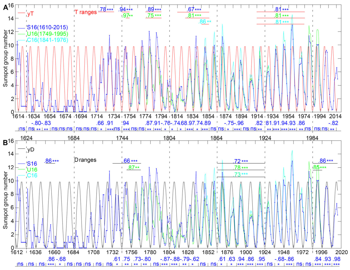
Subsequently, cycle-by-cycle correlation analyses were conducted for all the data on the yearly timescale (see Figure A1). In the case of S16 (blue curve), the correlation coefficients and significance levels for yT and yD cycles were provided at the bottom of Figure A1A and Figure A1B, respectively. The coefficients for U16 and C16 were not displayed because they were close to those of S16. Based on the positive correlation coefficients, T ranges (depicted by red lines in the upper part of Figure A1A) and D ranges (represented by black lines in the upper part of Figure A1B) were delineated for the three datasets, with the correlation coefficients and their significance levels (highlighted in various colors for different datasets) presented above these lines. Notably, there was a discernible pattern where yT and yD alternated in dominance in different 60-year sexagenary cycles after 1804. Moreover, during the sexagenary cycle from 1744 to 1804, both yT and yD demonstrated significant correlations with the SGN, while no clear pattern emerged before 1744.
On the monthly timescale, the U16 monthly data spanning Jan. 1749 to Dec. 1995 (N = 2964) exhibited significant correlations with yT (r = 0.39, p < 0.0001), yD (r = 0.08, p < 0.0001), myT (r = 0.27, p < 0.0001), and myD (r = 0.06, p < 0.001), but not with mT or mD. Meanwhile, the C16 data covering Jan. 1841 to Dec. 1976 (N = 1632) showed significant correlations with yT (r = 0.36, p < 0.0001), yD (r = 0.09, p < 0.001), myT (r = 0.26, p < 0.0001), and myD (r = 0.07, p < 0.01), but not with mT or mD (Table A1, items 4 and 5).
On the daily timescale, the U16 daily data from Jan. 1, 1749, to Dec. 31, 1995 (N = 90,214) demonstrated significant correlations with yT (r = 0.36, p < 0.0001), yD (r = 0.09, p < 0.0001), myT (r = 0.25, p < 0.0001), myD (r = 0.07, p < 0.0001), dmyT (r = 0.20, p < 0.0001), and dmyD (r = 0.06, p < 0.0001). Additionally, weak negative correlations were observed with mT (r = −0.01, p < 0.05), but not with mD, dT, or dD. The C16 data, covering Jan. 1, 1841, to Dec. 31, 1976 (N = 49,673), displayed significant correlations with yT (r = 0.33, p < 0.0001), yD (r = 0.08, p < 0.0001), mD (r = 0.01, p < 0.01), myT (r = 0.23, p < 0.0001), myD (r = 0.06, p < 0.0001), dmyT (r = 0.19, p < 0.0001), and dmyD (r = 0.05, p < 0.0001), while no significant correlations were found with mT, dT, or dD (see Table A1, items 6 and 7).
Figure A1.
Sunspot group numbers (SGN) from various sources exhibited significant correlations with (A) yearly T (yT) or (B) yearly D (yD) waves. The two cosine waves were scaled by a factor of five for better visual comparison. Correlation coefficients and significance levels, depicted in blue for Svalgaard 2016 (S16), green for Usoskin 2016 (U16), and cyan for Cliver 2016 (C16) data, were presented in the figure. The lines in the upper part (red for the T range and black for the D range) delineated the periods where the data showed positive correlations with yT or yD. Vertical lines indicated the boundaries of the 60-year sexagenary cycles. * p < 0.05; ** p < 0.01; *** p < 0.001; ns indicates not significant.
References
- Pulkkinen, T. Space Weather: Terrestrial Perspective. Living Rev. Sol. Phys. 2007, 4, 1. [Google Scholar] [CrossRef]
- Haigh, J.D. The Sun and the Earth’s Climate. Living Rev. Sol. Phys. 2007, 4, 2. [Google Scholar] [CrossRef]
- Hathaway, D.H. The Solar Cycle. Living Rev. Sol. Phys. 2015, 12, 4. [Google Scholar] [CrossRef] [PubMed]
- Tobias, S.; Hughes, D.; Weiss, N. Unpredictable Sun leaves researchers in the dark. Nature 2006, 442, 26. [Google Scholar] [CrossRef] [PubMed]
- Petrovay, K. Solar Cycle Prediction. Living Rev. Sol. Phys. 2010, 7, 6. [Google Scholar] [CrossRef] [PubMed]
- Pesnell, W.D. Solar Cycle Predictions (Invited Review). Sol. Phys. 2012, 281, 507–532. [Google Scholar] [CrossRef]
- Pesnell, W.D. Predictions of Solar Cycle 24: How are we doing? Space Weather 2016, 14, 10–21. [Google Scholar] [CrossRef]
- Wang, Y. Re-analysis of tropical cyclone variability from February 1956 to February 2016 over the western North Pacific using the TianGan-DiZhi calendar. J. Geogr. Reg. Plan. 2017, 10, 309–316. [Google Scholar] [CrossRef]
- Wang, Y. Exploration of the Scientific Value in Chinese Traditional Culture – Taking Yinyang–Wuxing and Tiangan–Dizhi as Examples, 1st ed.; Jinan University Press: Guangzhou, China, 2022. (in Chinese) [Google Scholar]
- Temmer, M.; Veronig, A.; Hanslmeier, A. Hemispheric Sunspot Numbers Rn and Rs: Catalogue and NS asymmetry analysis. Astron. Astrophys. 2002, 390, 707–715. [Google Scholar] [CrossRef]
- Gleissberg, W. A long-periodic fluctuation of the sun-spot numbers. Observatory 1939, 62, 158–159. [Google Scholar]
- Gleissberg, W. The probable behaviour of sunspot Cycle 21. Sol. Phys. 1971, 21, 240–245. [Google Scholar] [CrossRef]
- Suess, H.E. The Radiocarbon Record in Tree Rings of the Last 8000 Years. Radiocarbon 2016, 22, 200–209. [Google Scholar] [CrossRef]
- Usoskin, I.G. A history of solar activity over millennia. Living Rev. Sol. Phys. 2017, 14, 3. [Google Scholar] [CrossRef]
- Solanki, S.K.; Usoskin, I.G.; Kromer, B.; Schüssler, M.; Beer, J. Unusual activity of the Sun during recent decades compared to the previous 11,000 years. Nature 2004, 431, 1084–1087. [Google Scholar] [CrossRef]
- Usoskin, I.; Gallet, Y.; Lopes, F.; Kovaltsov, G.; Hulot, G. Solar activity during the Holocene: The Hallstatt cycle and its consequence for grand minima and maxima. Astron. Astrophys. 2016, 587, A150. [Google Scholar] [CrossRef]
- Wang, Y. “Yangjiu Bailiu” Related to Flood and Drought Disasters on Large Time Scales and Its Calculation Method. J. Jiujiang Univ. (Natural Science Edition) 2018, 33, 1–6. (in Chinese). [Google Scholar] [CrossRef]
- Weng, W.; Zhang, Q. Tiangan Dizhi Jili Yu Yuce (The Heavenly Stems and Earthly Branches Calendar and Its Prediction), 1st ed.; Petroleum Industry Press: Beijing, China, 1993; pp. 60–101. (in Chinese) [Google Scholar]
- Rozelot, J.P. On the stability of the 11-year solar cycle period (and a few others). Sol. Phys. 1994, 149, 149–154. [Google Scholar] [CrossRef]
- Wilson, P.R.; Altrocki, R.C.; Harvey, K.L.; Martin, S.F.; Snodgrass, H.B. The extended solar activity cycle. Nature 1988, 333, 748. [Google Scholar] [CrossRef]
- Javaraiah, J. North–south asymmetry in solar activity: predicting the amplitude of the next solar cycle. Mon. Not. R. Astron. Soc. 2007, 377, L34–L38. [Google Scholar] [CrossRef]
- Ohl, A.I. Forecast of sunspot maximum number of cycle 20. Soln. Dannye 1966, 84. [Google Scholar]
- Feynman, J. Geomagnetic and solar wind cycles, 1900-1975. J. Geophys. Res. 1982, 87, 6153–6162. [Google Scholar] [CrossRef]
- Thompson, R.J. A technique for predicting the amplitude of the solar cycle. Sol. Phys. 1993, 148, 383–388. [Google Scholar] [CrossRef]
- Svalgaard, L.; Cliver, E.W.; Kamide, Y. Sunspot cycle 24: Smallest cycle in 100 years? Geophys. Res. Lett. 2005, 32, L01104. [Google Scholar] [CrossRef]
- Muñoz-Jaramillo, A.; Balmaceda, L.A.; DeLuca, E.E. Using the Dipolar and Quadrupolar Moments to Improve Solar-Cycle Predictions Based on the Polar Magnetic Fields. Phys. Rev. Lett. 2013, 111, 041106. [Google Scholar] [CrossRef] [PubMed]
- Dikpati, M.; de Toma, G.; Gilman, P.A. Predicting the strength of solar cycle 24 using a flux-transport dynamo-based tool. Geophys. Res. Lett. 2006, 33, L05102. [Google Scholar] [CrossRef]
- Kitiashvili, I.; Kosovichev, A.G. Application of Data Assimilation Method for Predicting Solar Cycles. Astrophys. J. 2008, 688, L49. [Google Scholar] [CrossRef] [PubMed]
- Paraskakis, N.; Hristopulos, D.T. Prediction of yearly mean sunspot number using machine learning methods. Stoch. Environ. Res. Risk Assess. 2025, 39, 3405–3432. [Google Scholar] [CrossRef]
- Svalgaard, L.; Schatten, K.H. Reconstruction of the Sunspot Group Number: The Backbone Method. Sol. Phys. 2016, 291, 2653–2684. [Google Scholar] [CrossRef]
- Usoskin, I.G.; Kovaltsov, G.A.; Lockwood, M.; Mursula, K.; Owens, M.; Solanki, S.K. A New Calibrated Sunspot Group Series Since 1749: Statistics of Active Day Fractions. Sol. Phys. 2016, 291, 2685–2708. [Google Scholar] [CrossRef]
- Cliver, E.W.; Ling, A.G. The Discontinuity Circa 1885 in the Group Sunspot Number. Sol. Phys. 2016, 291, 2763–2784. [Google Scholar] [CrossRef]
Figure 1.
Correlations between monthly northern and southern sunspot numbers and the yearly cosine waves. From June 1944 to Jan. 1984, the northern sunspot numbers (nSN) correlated significantly with the yearly T (yT) cosine wave. In contrast, from Feb. 1984 to May 2018, the southern sunspot numbers (sSN) correlated significantly with the yearly D (yD) cosine wave. Across the entire period, the difference between nSN and sSN correlated significantly with the difference wave (yT − yD).
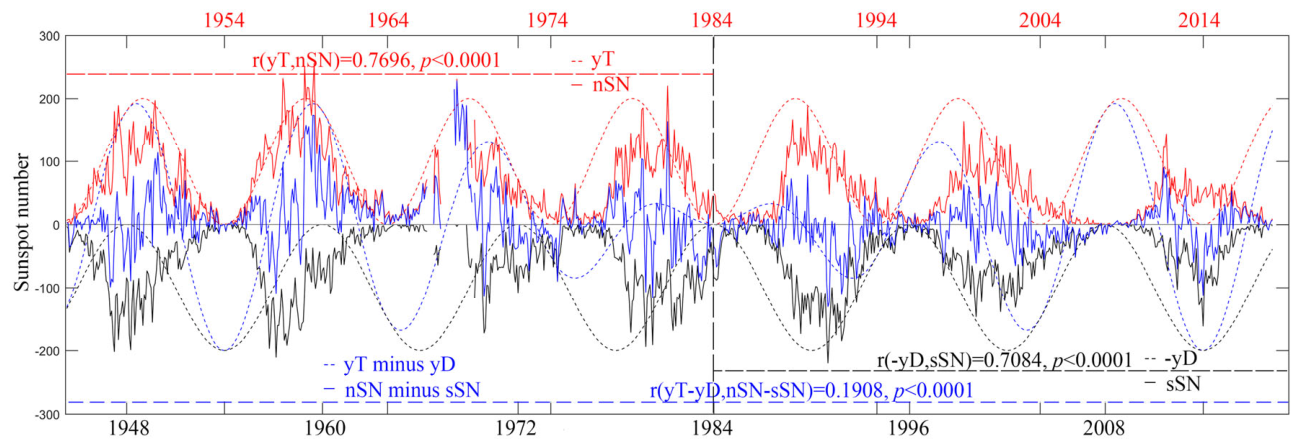
Figure 2.
Correlations between the spatial distribution of sunspots in the butterfly diagram and the θ values for yearly T (yT) and yearly D (yD) (see oblique dashed lines at the top and at the bottom, respectively). Correlation coefficients and significance levels (red for T, black for D) were shown alongside each cycle. Red lines at the top indicated the ranges with significant positive correlations for T cycles, and black lines at the bottom indicated those for D cycles, with corresponding coefficients and significance levels shown above or below the lines. Note: the yT and yD cosine waves were multiplied by 20 (in the north) and −20 (in the south), respectively, and plotted as background only for visual reference.
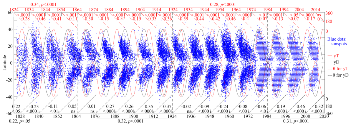
Figure 3.
Correlations between the raw polar magnetic field data and the yearly cosine waves. Three types of time ranges were presented: the entire range; the ranges before and after 1984; and the ranges defined by the 10-year T cycle (top) or the 12-year D cycle (bottom). Top: correlations between the raw northern data and the yearly T wave over different time ranges. Bottom: correlations between the raw southern data and the yearly D wave over different time ranges. Results for the filtered data were similar and were not shown. For more results, see Table 2 and Table 3. N, north; S, south; y, yearly; T, Tiangan; D, Dizhi; my, average of monthly and yearly waves.
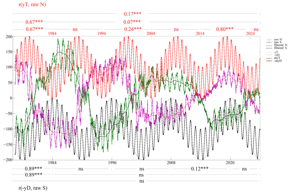
Figure 4.
Correlations between the raw northern polar magnetic field data and the yearly cosine waves over six time ranges segmented by the zero-crossing points of the filtered data. Three patterns emerged: (1) the yT-dominant pattern (Ranges 2 and 4), in which yT was significantly positively correlated with the northern data; (2) the −yD-dominant pattern (Ranges 3 and 6), in which −yD was significantly positively correlated with the northern data; and (3) the mixed pattern, which appeared in Range 1 (in which neither yT nor −yD was significantly correlated with the northern data) and Range 5 (in which both yT and −yD were significantly positively correlated with the northern data). Correlation results between the filtered northern data and the waves were also presented for reference.
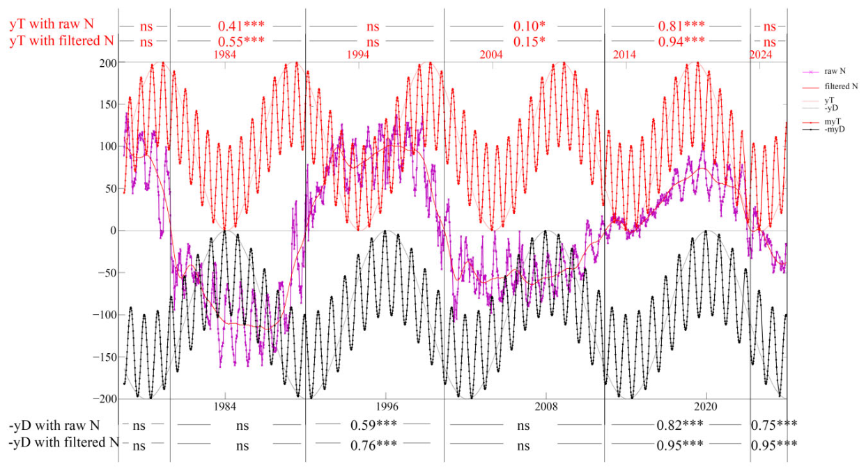
Figure 5.
Correlations between the raw southern polar magnetic field data and the yearly cosine waves over six time ranges divided by the zero-crossing points of the filtered data. Three patterns emerged: (1) the yT-dominant pattern (Range 3), in which yT correlated significantly positively with the southern data; (2) the −yD-dominant pattern (Ranges 2 and 4), in which −yD correlated significantly positively with the southern data; and (3) the mixed pattern, which appears in Ranges 5 and 6 in which neither yT nor −yD was significantly correlated with the raw southern data) and Range 1 (in which both yT and −yD were correlated significantly positively with the southern data). Correlation results between the filtered southern data and the waves were also presented for reference.
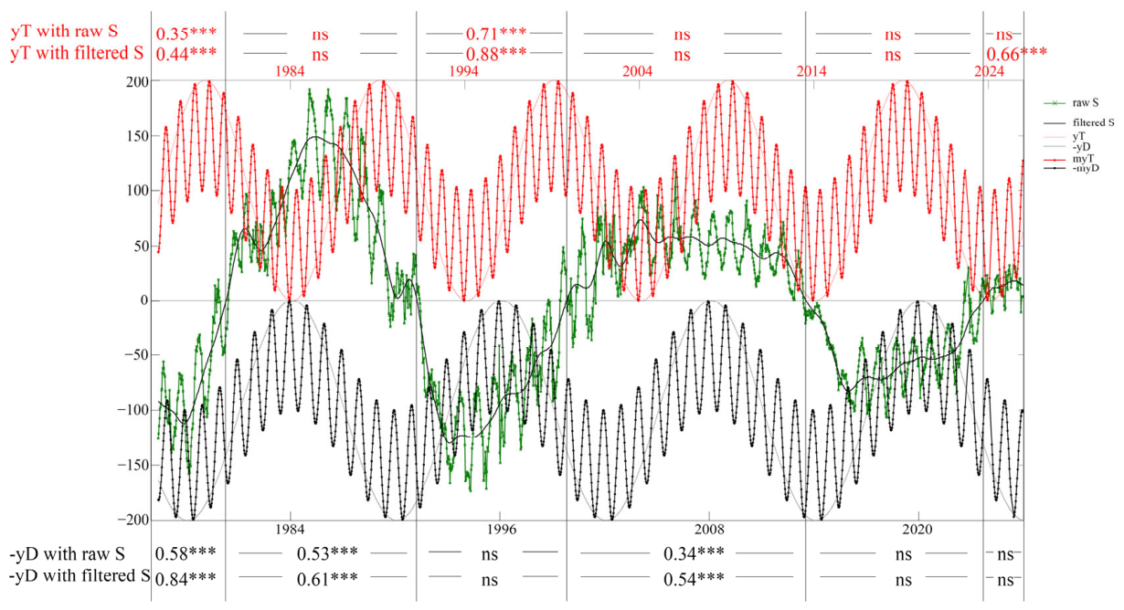
Table 1.
Correlation between KSO N–S monthly SN data and T/D waves.
| Time Range | Hemisphere | yT | -yD | mT | -mD | myT | -myD | yT minus yD |
|---|---|---|---|---|---|---|---|---|
| Whole period (1944—2018) | N and S | r = 0.44*** | NS | NS | NS | r = 0.32*** | NS | r = 0.19*** |
| June 1944—Jan. 1984 | N | r = 0.77*** | r = 0.35*** | NS | NS | r = 0.56*** | r = 0.21*** | - |
| June 1944—Jan. 1984 | S | r = −0.54*** | r = −0.47*** | NS | NS | r = −0.38*** | r = −0.34*** | - |
| Feb. 1984—May 2018 | N | r = 0.16*** | r = −0.72*** | NS | NS | r = 0.11* | r = −0.51*** | - |
| Feb. 1984—May 2018 | S | NS | r = 0.71*** | NS | NS | ns | r = 0.48*** | - |
* p < 0.05; *** p < 0.001; NS, not significant; —, not calculated. Note: All tests with p < 0.0001 are reported as ***.
Table 2.
Correlations between the data and the waves for each 10-year interval.
| Hemishphere | 10-year intervals | Raw | Filtered | ||
|---|---|---|---|---|---|
| yT | -yD | yT | -yD | ||
| N | 1976.5.31-1984.1.30 | 0.67*** | — | 0.72*** | — |
| 1984.2.9-1994.1.27 | — | — | — | — | |
| 1994.2.6-2004.1.25 | 0.24*** | 0.89*** | 0.25*** | 0.95*** | |
| 2004.2.4-2014.2.1 | — | — | — | — | |
| 2014.2.11-2024.1.20 | 0.80*** | 0.78*** | 0.94*** | 0.91*** | |
| 2024.3.10-2025.12.20 | — | 0.76*** | — | 0.99*** | |
| S | 1976.5.31-1984.1.30 | — | 0.89*** | — | 0.94*** |
| 1984.2.9-1994.1.27 | 0.20*** | 0.35*** | 0.22*** | 0.35*** | |
| 1994.2.6-2004.1.25 | — | — | — | — | |
| 2004.2.4-2014.2.1 | 0.27*** | 0.49*** | 0.39*** | 0.70*** | |
| 2014.2.11-2024.1.20 | — | — | — | — | |
| 2024.3.10-2025.12.20 | — | — | 0.72*** | — | |
*** p < 0.001; —, no significant positive correlation (including non-significant or significantly negative results). Note: All tests with p < 0.0001 are reported as ***. The results for mT and mD were not shown as nearly all of them were not correlated with the data; the results for myT and myD were also not shown as their values were only slightly lower than those for yT and yD.
Table 3.
Correlations between the data and the waves for each 12-year interval.
| Hemishphere | 12-year intervals | Raw | Filtered | ||
|---|---|---|---|---|---|
| yT | -yD | yT | -yD | ||
| N | 1976.5.31-1984.1.30 | 0.67*** | — | 0.72*** | — |
| 1984.2.9-1996.1.27 | — | — | — | — | |
| 1996.2.6-2008.2.3 | 0.54*** | 0.39*** | 0.58*** | 0.42*** | |
| 2008.2.13-2020.1.31 | — | — | — | — | |
| 2020.2.10-2025.12.20 | 0.69*** | 0.89*** | 0.78*** | 0.99*** | |
| S | 1976.5.31-1984.1.30 | — | 0.89*** | — | 0.94*** |
| 1984.2.9-1996.1.27 | 0.37*** | — | 0.39*** | — | |
| 1996.2.6-2008.2.3 | — | — | — | — | |
| 2008.2.13-2020.1.31 | 0.10* | 0.12* | 0.10* | 0.11* | |
| 2020.2.10-2025.12.20 | — | — | — | — | |
* p < 0.05; ***, p < 0.001; —, no significant positive correlation (including non-significant or significantly negative results). Note: All tests with p < 0.0001 are reported as ***. The results for mT and mD were not shown as nearly all of them were not correlated with the data; the results for myT and myD were also not shown as their values were only slightly lower than those for yT and yD.
Table 4.
Correlations between the raw data and different waves over six time ranges segmented by the zero-crossing points of the filtered data.
Table 4.
Correlations between the raw data and different waves over six time ranges segmented by the zero-crossing points of the filtered data.
| Hemishphere | NO. | Time range | yT | -yD | mT | -mD | myT | -myD | yT-yD | myT-myD |
|---|---|---|---|---|---|---|---|---|---|---|
| N | 1 | 1976.5.31—1979.12.2 | — | — | 0.20* | — | — | — | — | — |
| 2 | 1979.12.12—1990.1.8 | 0.41*** | — | — | — | 0.24*** | — | — | — | |
| 3 | 1990.1.18—2000.5.15 | — | 0.59*** | — | — | — | 0.36*** | 0.18*** | — | |
| 4 | 2000.5.25—2012.6.1 | 0.10* | — | — | — | — | — | — | — | |
| 5 | 2012.6.11—2023.4.15 | 0.81*** | 0.82*** | — | — | 0.58*** | 0.55*** | 0.85*** | 0.68*** | |
| 6 | 2023.4.25—2025.12.20 | — | 0.75*** | — | — | — | — | 0.48*** | — | |
| S | 1 | 1976.5.31—1980.4.20 | 0.35*** | 0.58*** | 0.17* | 0.19* | 0.30*** | 0.31*** | 0.60*** | 0.46*** |
| 2 | 1980.4.30—1991.3.24 | — | 0.53*** | — | — | — | 0.37*** | 0.37*** | — | |
| 3 | 1991.4.3—1999.10.28 | 0.71*** | — | — | — | 0.42*** | — | 0.37*** | 0.13* | |
| 4 | 1999.11.7—2013.7.16 | — | 0.34*** | — | — | — | 0.24*** | 0.15*** | 0.09* | |
| 5 | 2013.7.26—2023.9.12 | — | — | 0.13* | — | — | — | — | — | |
| 6 | 2023.9.22—2025.12.20 | — | — | — | — | — | — | — | — |
* p < 0.05; *** p < 0.001; —, not significant or negatively correlated. Note: All tests with p < 0.0001 are reported as ***; the correlation coefficients for the filtered data were similar to those for the raw data (shown above) and are therefore not shown.
Disclaimer/Publisher’s Note: The statements, opinions and data contained in all publications are solely those of the individual author(s) and contributor(s) and not of MDPI and/or the editor(s). MDPI and/or the editor(s) disclaim responsibility for any injury to people or property resulting from any ideas, methods, instructions or products referred to in the content. |
© 2026 by the author. Licensee MDPI, Basel, Switzerland. This article is an open access article distributed under the terms and conditions of the Creative Commons Attribution (CC BY) license.
Copyright: This open access article is published under a Creative Commons CC BY 4.0 license, which permit the free download, distribution, and reuse, provided that the author and preprint are cited in any reuse.