

Submitted:
05 October 2026
Posted:
09 October 2026
You are already at the latest version
Abstract
Housing insecurity is a critical aspect of understanding public health. To date, most work concerning housing insecurity focuses on urban environments with little research on rural conditions and the potential differences that exist between these environment. This leads to a fundamental question: how does housing insecurity change as we progress across the rural-urban continuum? To tackle this question, we considered several measures derived from the 2020-2024 5-year American Community Estimates and performed cluster analysis and association rules mining on a set of seven risk factors. We then further broke the analysis down based on the RUCA codes established by the US Department of Agriculture at the census tract geometry level. The results show that various housing insecurity factors predict others to varying degrees, based on rural/suburban/urban characteristics, with flow destinations (more urban settings) having different interaction profiles than flow providers (more suburban settings) and the most rural locales. The RUCA code provides a consistent pattern based on flow-rate to a central location. Connections to the extant literature about predictive mechanisms between subfacets are made. These differences and patterns have implications for policy and remediation, suggesting a typological approach to housing insecurity services based on aspects of the rural-urban continuum (a geospatial concept) and critical demographic data (a socioeconomic concept).
Keywords:
housing insecurity
; rural-urban continuum
; cluster analysis
; association rules mining
; geographic flow
1. Introduction
The rural-urban continuum is an important sociological and human geographic phenomenon that has become a core variable in social sciences over recent years. While historically, the rural-urban continuum was meant as a dichotomous concept, it is more accurate and useful to conceptually describe it as a progression [1,2]. Studies of the rural-urban continuum can be seen across the social sciences, with applications to psychology [3], geographic change [4,5], demography [6], political science [7,8,9,10], sociology [11], economics [12,13], and criminology [14,15]. In short, while we as a society tend to acknowledge urban and rural areas, we operationalize these concepts in overly simplistic ways; rural areas are often defined as simply non-urban despite a wide variation geographical and social factors among areas classified in this way [16]. This leads to significant challenges in understanding the natural progression of socio-economic and/or socio-cultural phenomena. And as Lichter and Brown [17] note, rural and urban areas, while distinct across many metrics, are also interdependent and face a range of similar social problems.
In the United States, a series of codes were developed by the U.S. Department of Agriculture [18] in the 1990s and were reevaluated after the decennial census to characterize this rural-urban continuum (Table 1). This process allowed for the designations of areas to change with their present reality through time, representing temporal evolution. A map of current RUCA codes for US census tracts is shown in Figure 1.
In research on social issues, urbanness is often the dominant paradigm. As a result those with lived experiences sometimes express self-identities that are at odds with the RUCA designations [19]. Part of this issue is the fundamental way in which RUCA codes are inferred from census and American Community Survey data. Overall, there are a lot of areas that when you change how they are modelled, a different outcome arises. However, tract level analysis shows about 97% convergence between types [20]. This fundamental assertion makes understanding how social phenomena occur within these groups even more tantamount. Acknowledging the full continuum allows for creativity in policymaking by parsing more nuanced perspectives to match solutions to concepts of underlying reality, impacting areas across the continuum more appropriately to their own context.
When we think about the RUCA code designations, it is important to recognize that RUCA codes are not about population density; rather, they are about the flow of people to work and centralized services. A couple of prime examples in Table 1 are Portland, ME (1), Standish, ME (2), Augusta, ME (4), Presque Isle, ME (7), and Farmington, ME (10). All of these locations house a college or university. Portland itself is a sufficiently large urban city to be defined as a metropolitan core. Residents of Standish typically commute to Portland. Augusta represents a micropolitan area that people commute to. Presque Isle represents a small town that people commute to. Farmington represents a rural enough area that any commuting does not enter a micropolitan area. The population is not the main focus for those areas that give flow, but rather for those that receive it. For example, Livermore Falls (3) has less than half of the population of Farmington (10), yet it has a more urban-like RUCA code. The difference is that Livermore Falls flows into Lewiston-Auburn (1), whereas Farmington pretty much sustains itself and is not incorporated as a city.
Metropolitan, micropolitan, and small-town areas serve as hubs of activity, and because of this, they are more likely to have some semblance of centralized resources that surrounding communities will leverage. This is not universally restrictive. For example, Skowhegan, ME has a functioning hospital and medical offices, despite being classified as a 10. In Skowhegan is some necessity to having these functions due to its location in Somerset County with respect to other communities which cannot on their own support that type of resource. This can lead to fiscal inefficiencies in the provision of resources in rural areas that are otherwise straightforward in urban ones, a concept that is critical to understand in housing insecurity research.
Housing insecurity is a critical concept in understanding public health, where housing is considered an important social determinant of health [21]. Coleman-Jensen, Steffen, and Whitley [22] describe housing as a “somewhat lumpy bundle of services” that consists of “a package of basic shelter, neighborhood security and amenities, access to transportation and social networks, personal consumption, productivity potential, and financial investment potential” (270). Just as housing itself is complex, so are the broad range of social outcomes with which it is associated. While housing insecurity is often most strongly associated with homelessness among the general public [23], it is a far more structurally complex issue,
Swope and Hernandez [21] have convincingly documented the health impacts of insecurity housing using the four C’s framework: Cost, Condition, Consistency, and Context. The four C’s framework gives some structure to organizing the “somewhat lumpy” [22] aspects of housing. The first C is cost, which draws attention to the importance of the cost-burden of housing. If community members pay most of their income to housing (e.g., rent, utilities, maintenance costs), then very little is left to cover other costs (e.g., food, medicine, transportation). Condition examines the quality of the housing, where overcrowded or dilapidated housing can negatively impact health and wellbeing. Consistency draws attention to the instability of involuntary moves (e.g., evictions, couch surfing) and the negative impacts this can have on health. Finally, the fourth C is context, which focuses on the community or neighborhood context of housing. If a community is unsafe, unwalkable, or lacks adequate sources of healthy food, this can be detrimental to health [21]. Swope and Hernandez make a strong argument for broadening research and understanding on housing insecurity to conceptualize it as a continuum of housing struggles, where homelessness is included as an unsheltered expression of this continuum [21].
For the most part, the overwhelming majority of housing insecurity research is anchored in urban areas [16], whereas there is very minimal research into the effects of housing insecurity in rural communities, although the volume of it is increasing [24,25,26,27,28,29]. The existing body of literature on rural housing insecurity indicates that assumptions derived from research on urban homelessness cannot be applied wholesale to rural areas [16,24,25,26,27]. For example, methodologies of measuring rates of homelessness typically applied in urban areas do not adequately capture the extent of the problem in rural areas [25]. Unsheltered and other types of housing insecurity tend to be more hidden [26] and less publicly recognized [27] in rural areas. Gleason et al. [26] have also stressed the need to appreciate the unique housing challenges of different rural areas. They used key informant interviews to explore housing insecurity across four different rural areas in Maine and found that the differing histories and geographies of these areas likely shaped differences in housing issues across the areas. Because rural housing insecurity is under researched, there are still large gaps in our understanding of the diverse risks, contours, and needed interventions in rural areas [26,27]. Montañez’s [30] ethnographic study of Taos is an example of the complex ways in which housing insecurity reflects many aspects of the “four C’s,” and how these struggles are shaped by the specificity of the particular ruralness of Taos. In this location, a gentrifying rural community faced housing shortages due to residential mobility and in-migration, rising costs, and increased incidence of AirBnBs. Montañez noted distinct patterns in how different ethnic groups navigated housing insecurity, with long-term Hispanic residents being more likely to rely on kinship networks and strategies such as renting rooms or trailers on family land, which can provide barriers to applying for aid, and using robust social networks to learn of resources. White newcomers, however, were more likely to engage with formal services and live in vehicles or shelters. Coleman-Jensen, Steffen and Whitley [22] also cite survey data that suggest the tendency to rely on family is more common among the rural housing insecure, whereas urban individuals are more likely to appeal to friends, emphasizing how different social networks and family structures are more or less salient in different spatial contexts.
Speaking more broadly, there are a range of reasons why we might expect rural and urban areas to have different levels of risks across the four C’s of housing insecurity. Some rural areas, for example, have been experiencing population loss (e.g., outmigration) for decades, while others have started to see marked increases in population due to in-migration of retirees and tourist populations [31]. Rural areas also have higher rates of homeownership than the national average, and generally have lower home prices, on average [32]. However, despite this increased affordability and availability, rural areas have higher rates of poverty than the national average [33]. These trends also vary significantly by region as well as rural-urban status [22].
Because of the need to better understand the spectrum of housing insecurity risks in and its intersection with rural-urban dynamics, we propose the following research questions: does the rural-urban continuum relate to shifts in rates of risk across the four C’s of housing insecurity? Do RUCA codes 1, 4, and 7 (anchoring hubs) behave similarly to one another (or more similarly to one another) than do other codes? Would that behavior pass down to the percentile exchange groups (2, 5, 8 and 3, 6, 9 respectively)? How does code 10, the most rural code and one outside of an explicit commuting area, relate to any of these? Prior research has suggested that the more rural an area is, the more likely that the housing insecurity strain is targeted to one or two of the 4 C’s as opposed to systemic failure [26].
In this paper, we tried to predict risk of housing insecurity based on publicly available data regarding demographic information across the United States that reflect the 4 C’s of housing insecurity. To accomplish this, we used several data mining techniques to create an ensemble approach to risk assessment. For each dimension, we asserted a risk for the individual tract. From this, we constructed intersectional profiles of the 4 C’s and compare incidence rates of risk based on the RUCA code designations. The goal of the study was to understand how our risk assessment measure correlates with the structure of the rural-urban continuum. Furthermore, we endeavored to consider how urban areas might be able to learn from the profile of rural areas and similarly how an area going through a transition in the rural-urban continuum might project to appear within those dimensions.
2. Materials and Methods
Using the tidycensus package from R, a total of 85 2020-2024 ACS 5-year variables were extracted at the census tract level to capture the four C’s of housing insecurity. A series of eight concepts were used to characterize areas motivated by extant literature [16]: economic diversity, demographic diversity, housing cost, housing quality, residential mobility, household factors, and housing type. Of particular note in this dataset is that a small set of census tracts from Brentwood, NY and Wyandanch, NY are missing due to an interviewing error from the US Census Bureau. These datapoints have been removed.
A series of measures were constructed to address each of these areas by combining relevant ACS measurements:
-
Economic diversity
- o Sullivan index of economic diversity, GINI index, proportion of workers in below average economic wage categories
-
Demographic diversity
- o Proportions of white, women, and children, Sullivan index of racial diversity
-
Housing cost (Cost)
- o Mortgage, owner non-mortgage, and renters paying over 30% of their income (burden)
-
Housing quality (Condition)
- o Occupied incomplete kitchen or plumbing
- o All incomplete kitchen or plumbing
-
Residential mobility (Consistency)
- o Same house, moved within county, moved within state, moved out of state
-
Household factors
- o Households with 3 or more workers, households without investment income, households with no other income, households with no vehicle, households with no wages, households with public assistance, households with Social Security Insurance, households with workers with no vehicle
-
Housing type
- o Renter/owner ratio, renters broken down by single, 2-4, 5+ units, mobile homes, and unconventional housing.
The USDA RUCA codes table linking census tracts to the rural-urban continuum for the 2020 decennial US Census were joined to the remaining data columns from the ACS data.
In each of the various groups, k-medoids clustering was employed to determine clusters of high-, medium-, and low-risk of housing insecurity based on how the literature characterizes housing insecurity challenges using silhouette metrics [34]. For example, an area with high economic diversity (i.e., a varied job profile) has better economic resilience as compared to an area with a lower economic diversity is susceptible to employment and income challenges, thus the cluster with the most economic diversity is labelled lowest risk and the one with the least is labelled as highest risk.
Association rules mining was conducted on these associated risk levels to determine if there are patterns within the risk levels. Association rules are formed when there are several comorbidities that tend to be found in concert, increasing the likelihood of the occurrence of the other from the base proportion, evaluated by measures such as support, confidence, lift, gain, and conviction [35]. It is important to consider these concepts to see if the nature of comorbidities is changing along the rural-urban continuum.
To achieve an understanding of the impact of the rural-urban continuum on housing insecurity, these approaches are further analyzed with respect to the RUCA codes. We approach this problem from two different perspectives:
- Central locations (1,4,7) compared to various feeding levels (2,5,8), (3,6,9)
- Size of the centralized hub (1,2,3), (4,5,6), (7,8,9), (10)
3. Results
Utilizing the RUCA codes and various ACS data columns, we present a multi-pronged analysis of the Rural-Urban Continuum across housing insecurity dimensions. In Section 3.1, we create clusters of risk of housing insecurity across seven characteristics. In Section 3.2, we look at how the Rural-Urban Continuum is distributed across the various risk factors. In Section 3.3, we look for comorbidities of housing insecurity risk. In Section 3.4, we look for changes in those comorbidities based on RUCA codes.
3.1. Clusters of Risk
Using the cluster library in R, the ACS data of each census tract with a complete record was processed using the clara function for each of the seven identified dimensions of potential housing insecurity. The clara function attempts k-medoids partitioning by taking samples of larger datasets and then propagating those results across the rest of the dataset a specified number of times. The model was run under an assumption of self-standardization (to account for the diversity of scales of measures compared to one another) and was based on 20,000 samples (~25% of the dataset). Because demographic data is inherently messy in terms of similarity, it is expected that there will be overlap between clusters. As such, we pay closer attention to the silhouette scores than the isolation scores [34]. Silhouette scores can range from -1 (totally random cluster) to 1 (totally isolated clusters). Silhouette scores above 0.7 are considered strong; above 0.5 are considered moderate, and above 0.25 are considered weak. The results of the clustering protocol are enumerated in Appendix A in Table A1, Table A2, Table A3, Table A4, Table A5, Table A6 and Table A7. Silhouette graphs are presented in Appendix A in the odd numbered Figure A1Figures –Figure A14. PCA plots are presented in Appendix A in the even numbered Figure A1, Figure A2, Figure A3, Figure A4, Figure A5, Figure A6, Figure A7, Figure A8, Figure A9, Figure A10, Figure A11, Figure A12, Figure A13 and Figure A14. Table 2 summarizes the silhouette scores for the various clusterings from Table A1, Table A2, Table A3, Table A4, Table A5, Table A6 and Table A7.
Figure 2, Figure 3, Figure 4, Figure 5, Figure 6, Figure 7 and Figure 8 show the spatial distribution of each of the clustering outputs within the coterminous United States. Each of the figures shows substantive variation, suggesting that a typological approach is likely to better serve practitioners.
3.2. Distribution of Risk Across RUCA Codes
Areas with different RUCA codes are fundamentally different by their geographic and communal nature. It is thus important to understand how the classifications break down across RUCA codes. We examined percentages to address this phenomenon as it is disproportionately likely to see census tracts at levels 1, 4, 7, and 10. The resulting tables are found in Appendix B. As a means of summarizing, Table 3 records the proportion of high risk tracts in each risk category.
3.3. Comorbidities in Housing Insecurity Risk Factors
An association rules mining procedure [35] was applied to the dataset to determine if there are risk factors that seem to predict one another at high levels. In Table 16, the list of association rules between high risk classifiers that have at least a confidence of 0.3 are presented. A lift exceeding 1 suggests that the rule predicts a stronger affinity with the antecedent (lhs) than the overall affinity of consequent (rhs) in the dataset at large. To interpret the following tables, we consider the first row of Table 4. The first row of Table 4 has LHS of ROC=H, RHS of HHFC=H, Support of 0.003, Confidence of 0.634, Coverage of 0.005, Lift of 2.478, and Count of 279. In an association rule, the LHS (left-hand side) is called the antecedent. The aim of the analysis is to see how the presence of the antecedent influences some other piece of information. The RHS (right-hand side) is called the consequent is that second piece of information. Support reflects the proportion of the overall dataset that has the two concepts together. Count reflects the raw number within the dataset. Coverage reflects the proportion of rows in the dataset that include LHS, and must be at least as large as Support because Support adds further restriction. Confidence is the conditional probability that a row that contains LHS also contains RHS, computed by dividing Support by Coverage. Lift represents the strength of the rule from the perspective of how much of a gain is produced from the information, namely Confidence/Coverage for RHS. In the case of the first row of Table 4, knowing that ROC is high risk scales the support for HHFC being high by a factor of almost 2.5, suggesting there is a strong connection between these concepts in that particular order. It is possible for Lift to be less than 1, suggesting that knowledge of LHS makes RHS less likely. There are a few instances of this within Section 3.3 and Section 3.4. In total, this line of data suggests that ROC = H is not very prevalent (this is also observed in Table A7 and B7), but when it is, it provides evidence that HHFC = H will appear disproportionately relative to its normal rate.
To place the rules in Table 4 in context, there are 80,855 records for which every measure can be computed. These rules are the only ones in which the antecedent produces the consequent at least 30% of the time (confidence). The largest number of an occurrence of this is less than 1 out of every 9 times. These rules also demonstrate that in four cases, the antecedent more than doubles the rate of occurrence of the actual phenomenon.
Similar to an association rule, it is also important to get sheer counts of the number of times a census tract has a certain number of comorbidities. That insight is shown in Table 5.
Table 5 demonstrates clearly that the majority of tracts have few high risk classifications, but a select few have a very large number of them. Figure 9 shows how these counts distribute through space.
Both Table 4 and Table 5 however treat all census tracts as equal; RUCA codes suggest there are fundamental differences between census tracts that center on surrounding context. In Section 3.4, we break this down further.
3.4. RUCA Codes and the Impact on Comorbidities
In order to get a better understanding of the impact of the RUCA codes on comorbidities, we repeat the analysis from Section 3.3 on each RUCA code subset of the data. The association rules results are shown in Appendix C and summarized in Table 6. Tables C1-C10 do not immediately show patterns in their relative size or their components. To get a better understanding of their similarity, we have compiled a compendium table (Table 6) that shows where the various combinations occur.
Table 6 shows that RUCA code 1 is the dominant feature in producing association rules. This is unsurprising as it has 68% of the dataset. When we remove the effect of RUCA code 1 by letting each RUCA code be its own set, it becomes easier to see that some associations are hidden by the most urban census tracts. The association rules analysis provides a glimpse into which factors occur together in only urban environments, only rural environments, or in any combination. It also reveals those that occur in many conditions.
4. Discussion
There are numerous points of interest to discuss relative to the analyses in Section 3. Section 4 is thus broken down based on the dimension of the analysis in question.
4.1. Clustering Procedure
Table 2 and Appendix A highlight the difficulties in trying to predict risk factors on large scales. The ability to find segregated categorizations in multi-dimensional factors is very difficult [16]. One concept did however occur over and over again: the lowest risk category is the one that is the most isolated, having larger silhouette scores. This is a strong indicator that risk factors are diverse and localized, as shown by Gleason et al. [26].
4.2. Clustering Procedure Across RUCA Codes
The most striking finding in Section 3 is the parallels between the codes, based on their status as “core” or commuting outflow areas as exhibited in Appendix B and Table 3 as well as in Table 7 and Table 8. The data did not cluster in risk factors at ends of the spectrum as one might expect with a clear “rural” vs. “urban” dichotomy. Instead, similar types of places (e.g., flow centers) looked more like their functional counterparts than their spatial (e.g., rural or urban) counterparts. This indicates another example of rural-urban alignment and interdependency [5]. Another noteworthy finding was the comorbidity count for RUCA code 10. From the perspective of having any morbidity with respect to housing insecurity or comorbidities, RUCA code 10 seemed to behave more like the rural codes that flow into RUCA code 7 than the RUCA codes 1, 4, and 7. This indicates that the most rural places in the U.S., especially those that are not within easy commuting distance to employment centers face a range of social challenges, from concentrated poverty and racial and ethnic segregation to becoming home to LULUs (locally undesirable land uses) such as prisons. This is the type of place that Eason [36] dubbed “rural ghettos.” These communities, with little economic opportunity and few ties to regional economies become stigmatized and economically depressed, presenting them with challenges somewhat similar to disadvantaged urban neighborhoods, but without the benefits of population density, economies of scale, or public transportation to help mediate these conditions. This stands in contrast to those areas that flow into metropolitan (RUCA code 2-3) and micropolitan (RUCA code 5-6) areas which have the lowest rates of both morbidity and comorbidity. We might classify these communities conceptually as suburbs. In this sense, trends in the areas surrounding rural and urban centers seem to come together.
Appendix B and Table 3 show interesting patterns that relate to RUCA code designations. Economic diversity (Table B1) and household factors (Table B5) show a similar pattern where the rate of occurrence of a morbidity is strongest in flow centers and the rate of morbidity increases as the population of those flow centers decreases. In other words, high risk in economic diversity was highest in flow centers, with higher rates of high risk in economic diversity in smaller flow centers. We interpret this as inequality in wages and wealth being most prominent in flow centers, especially those with smaller populations (e.g., small towns). This reflects the reality that less than thirty percent of rural counties are classified as economically diverse, while a majority of metropolitan counties are [37]. Household factors, which also capture economic vulnerability (e.g., not having transportation or wages and using government benefits) are also more prominent in flow centers and especially prominent in smaller flow centers. What is notable is that this seems to demonstrate low population flow centers are likely to be areas of high service need with relatively few service resources [38]. For example, few of these areas are likely to have emergency shelters for housing [25].
Demographic diversity (Table B2) and renter/owner characteristics (Table B7) are strongest in flow centers and dissipate rapidly both with flow rate and as the size of the flow center declines. These concepts suggest a phenomenon predicted by population and centrality. Lee and Sharp [39] suggest that at the aggregate level this is true for demographic diversity, but is potentially dissipating and lacks spatial context; similarly, urban environments have far more reliance on rentals than do rural settings [40].
Housing costs (Table B3) and residential mobility (Table B6) represent problems that are strongest in flow centers, but the size of the flow center is largely irrelevant. Housing costs tend to relate to being in desirable locations, closer to amenities and infrastructure [41], and centralized locations fit this bill [42]. Residential mobility is of course predicated by being forced to move and/or having stock available with which to move. This requires sufficient units, again, likely in centralized places.
Finally, housing quality (Table B4) seems to be a morbidity characteristic of dispersal, with the rate of occurrence increasing as the flow center gets smaller but also having stronger signals in places that flow toward these centers. This fits in with trends related to the core-periphery model, where preference is given to centralized locations for value, and thus translates into lower quality moving away from the center (in this case, places with decreased amount of flow) [43].
4.3. Association Rules
Interesting patterns seem to arise within the association rules protocol across the identified factors of housing insecurity from Section 3.3 and Section 3.4 that can be seen by navigating Table 6 with an eye toward the structure of the RUCA codes. We emphasize that the interpretation of association rules can be confusing, so we reiterate that association rules relate categories to categories: an association rule exists when knowledge of one category meaningfully alters the rate of occurrence of another category (i.e., conditional probability). This is not the same as the rate of a measure being positively correlated with the rate of another measure (i.e., regression). It is important to note that often times regression arguments can be helpful in providing support for why a category might spike in conditional probability. As such, we endeavor to provide instances where such spikes are supported by phenomenon found in the literature.
Renter/Owner characteristics (ROC) never occurs as a consequent in an association rule, either within the whole dataset or within the various subsets by RUCA code. This is not necessarily due to it not being a legitimate comorbidity with other concepts, but rather a consequence of the overall size of the high risk cluster, seen in Table A7 and B7. It does, however, serve as an antecedent, in each case predicting a rule that is relevant to flow centers. Its relationship to residential mobility (RMC) is relevant to all flow centers. In all flow centers (RUCA 1, 4, and 7) the high risk group of renter/owner characteristics substantively increases the rate of high risk in the residential mobility dimension. This makes sense as flow centers have higher rental rates [40] and eviction is a much larger problem in these areas than it is in rural environments [44]. ROC’s relationship to economic diversity (EDC) is relevant to metropolitan and micropolitan flow centers, with high risk renter/owner characteristics predicting high risk economic diversity at a stronger rate than normal; this might be caused by the relationship between the GINI index and rental affordability in metropolitan areas [42] combined with higher rates of renting in urban environments [40]. ROC’s relationships with demographic diversity (DDC), housing costs (HCC), and household factors (HHFC) are all relevant to metropolitan centers. This is a clear indication that the overall size of the flow center changes how ROC is found in situ. ROC and housing quality (HQC) do not seem to influence one another notably, which is likely a side effect of the sheer lack of volume of ROC risk in rural environments within the clustering outcome.
Flow centers seem to hold a key place in the risk factor comorbidities. Several pairs of morbidities occur only between flow centers.
High risk in the housing quality dimension appears to predict high risk in the economic diversity dimension. This suggests that substandard housing seems to place itself around areas with lesser economic diversity, higher incidence rates of poverty, and general income inequality. This would make sense across the spectrum. Areas that are characteristically central are likely to have income inequality issues, and housing quality can afflict all areas (e.g., run-down rural communities that have experienced significant economic shifts like in West Virginia [45] or cities with historical development changes such as Detroit and Flint, Michigan [46]).
High risk in special household factors appears to predict high risk in housing costs in all flow centers. This is a difficult area to discuss because many of these factors are about transportation, income, or benefit utilization. An example of this concept is found in practices by landlords to offset benefits for housing with overpriced rentals [47].
In metropolitan and micropolitan flow centers, high risk in special household factors appear to predict high risk in residential mobility. It is likely that areas in the high risk category for special household factors wind up with issues that can lead to eviction, predicating movement.
In metropolitan flow centers, high risk in the residential mobility dimension appears to predict high risk in the demographic diversity dimension. Because rents are more expensive and prevalent in urban areas [40,44] and urban areas are much more associated with demographic diversity [39], such an association makes sense. This is not, however, universal. Certain ethno-racial groups are actually highly immobile [48], however, eviction serves as a harrowing contrast to this, where those same immobile groups have stunning eviction rates [49]. Similarly, high risk in residential mobility appears to predict high risk in housing costs in metropolitan flow centers. Urban costs are skyrocketing, and this has had a substantive impact on evictions amongst urban poor [44].
In metropolitan flow centers, high risk in the economic diversity dimension appears to predict high risk in the demographic diversity dimension. This is a fairly clear connection to the concept of redlining [50], using economic means related to income inequality to segregate communities, which disproportionately impacts minority populations in the urban centers of the US. Similarly, economic diversity appears to predict high risk in the housing cost dimension, suggesting that income inequality is higher where housing is more expensive [51].
In metropolitan flow centers, high risk in the housing quality dimension appears to predict high risk in housing costs and also high risk in the demographic diversity dimension. Housing quality and cost seem to reflect a surprising juxtaposition, but Desmond [52] argues that renters in lower-income urban areas often pay disproportionate to unit worth as landlords jack prices to offload risk of renting in that environment. Demographic diversity is not nearly as surprising as with the sheer amount of income inequality in minority populations combined with the redlining effect would lead to these risk factors aligning in urban environments.
In metropolitan flow centers, high risk in special household factors appears to predict high risk in demographic diversity. One of the components of the special household factors concerned lack of access to personal transportation. There are significant examples of disparities in public transportation access in minority communities [53].
Two different high risk categories appear to predict high risk in residential mobility in micropolitan areas: high risk in economic diversity and high risk in housing costs. Micropolitan areas (like rural areas) are often not the primary target of studies [54], so exploring this linkage is a suggestion for future study.
Residential mobility and economic diversity have an interesting relationship in that they are the only pair which combines the flow centers with the areas that flow highly to them. This is a pairing that we would expect to see in flow centers due to the economic issues and eviction factors [44]. However, the addition of the high flow communities is insightful. Research suggests that suburban areas are shrinking [55]. Also, research suggests that poverty is on the rise in suburbs [56], which could also contribute to this linkage.
High risk in residential mobility appears to predict high risk in housing quality in sub-micropolitan flow providers as well as purely rural tracts. This suggests something of importance: the reason for movement in flow centers is likely centered around cost concerns, whereas in lesser populated areas, the issue is about the quality of the house itself, emblematic of the core-periphery model. Recent studies show that rural areas suffer from housing quality issues more so than their urban counterparts [57].
In both flow centers and rural areas, high risk in residential mobility and high risk in housing quality appear to predict high risk in special household factors. This would suggest that the necessity of moving and challenges with respect to housing quality impact households with specific needs across the board with respect to places that are their own emphasis. This is not surprising as one of the factors in the list is about lack of transportation, meaning that that family would be dependent upon where they live to sustain them economically.
In both flow centers and rural areas, high risk in housing cost predicts high risk in economic diversity. While costs in urban areas are spiraling out of control, the same is true in rural areas [58]. This fits in nicely with the concept of rural gentrification [59].
In both flow centers and rural areas, high risk in special household factors appears to predict both high risk in economic diversity and housing quality. Special household factors are often associated with poverty which knows no real spatial bound, and housing quality can be compromised in several locations.
In sub-micropolitan areas, high risk in demographic diversity appears to predict high risk in both housing quality and special household factors. This would suggest that as population areas get smaller, diverse populations wind up in more distressed communities [37].
In rural areas, high risk in housing cost appears to predict high risk in housing quality. This appears consistent with the idea of the core-periphery model [43], but also consistent with the idea of the growth of the AirBnB market [30].
There is one virtually universal rule (other than RUCA code 2): high risk in housing cost predicts high risk in special household factors. RUCA code 2 is significant in that it is the most prototypically suburban area.
Several rules are hidden when looking at the entire dataset. Table 6 has 12 combinations that are undiscovered until filtering the dataset into subsets by RUCA codes, clear evidence for nuance in factor combinations.
The intricacies of the relationships between various factors have an important role to play in the construction of policies geared at remediation of housing insecurity challenges. The lack of universality of the association rules shows that we must be cognizant of the types of comorbidities that are mutually predicted in areas and use that knowledge to better situate services to meet the needs of communities, be they rural, suburban, or urban. Moreover, these complicated association rules suggest that we should pay attention to both population size and flow related to economic centers of various sizes when parsing need and policy solutions.
5. Conclusions
The overall picture of the results in Section 3 presents a pattern across the rural-urban continuum in the form of the USDA RUCA codes. Flow centers and flow percentages tend to drive the pattern in the dataset for the existence of risks for housing insecurity. Only in isolated categories do we find a general decline or spike based on the relative size. This means that RUCA codes 1, 4, and 7 (core areas) behave more similarly to one another than they do to other codes. RUCA codes 2, 5, and 8 (high commute into core areas) are similarly related; as are RUCA codes 3, 6, and 9 (low commute into core areas). When searching for comorbidities, after getting to rural RUCA codes, the comorbidity profile more closely resembled flow centers. This is not all that surprising as rural communities often have to fend for themselves. Associations between specific comorbidities are dictated largely by the set of urban census tracts, but patterns exist outside of this. Particular comorbidities only come into focus when the effects of the urban tracts are removed as they are disproportionately represented as efforts are made to try to control the populations of census geometries at the tract level to be relatively equal in population where possible. To our knowledge, only Byrne et al. [60] have attempted to compare community level risk factors for housing insecurity (specific to homelessness) nationwide. Their study used U.S. Department of Agriculture’s (USDA) Economic Research Service definitions of rurality, comparing metropolitan and non-metropolitan areas on factors associated Housing and Urban Development Continuum of Care homeless counts. They did find some differences in morbidity factors between rural and urban areas. For example, rent levels and unemployment were stronger predictors of homelessness in non-metro areas. However, the findings described in the present study call into question the validity of approaching rural and urban housing risks in a dichotomous way. Our findings suggest that risk factors for housing insecurity might be patterned along dimensions more related to proximity to an economic core than strictly along metro/non-metro lines.
Interestingly, it seems that the difference between rural, suburban, and urban arise when we address comorbidity prediction. Some characteristics are predicted well as comorbidities in urban settings; others have nuanced predictions that do better in rural, suburban, or urban (and in some cases combinations). While flow appears to be the determining factor for prevalence of high risk measures for housing insecurity, the differences across the continuum that relate to size tend to have a greater effect on prediction of associated problems. This seems to indicate that risk of housing insecurity may occur along multiple dimensions related to both economic flow to centers and the size of the communities in question, with the intersection of these factors appearing to pattern risk in complicated ways.
Gleason et al. [26] have recommended that research on rural housing move towards developing a typology of patterns for rural housing insecurity. Overall, the findings of the present study illustrated clear support for the argument that rural-urban differences exist along a continuum and not a binary. As demonstrated consistently throughout the results, RUCA codes 1, 4, and 7 (core areas) are remarkably consistent in terms of their housing insecurity risk factors, despite being in very different areas of the rural-urban population size continuum. This same pattern plays out for codes 2, 5, and 8 (high commute to core areas) as well as 3, 6, and 9 (low commute to core areas). We also found notable housing insecurity risks for code 10, indicating that the very rural areas in the U.S. that are not within easy commuting distance to employment centers face higher risks for a range of social challenges. These findings highlight the importance of thinking beyond “rural” or “urban” labels and simple population thresholds and thinking instead about the social and economic dimensions of places and how those characteristics may provide a more useful, place-based typology for understanding important social problems such as housing insecurity.
This study overall highlights that understanding housing insecurity at the typological level is more than just an exercise in understanding demography; a typology of housing insecurity should also include the role of the rural-urban continuum, specifically aspects of the place’s regional role and size. Housing insecurity challenges present differently under different conditions. The risk profiles of areas based on their rural-urban continuum position can differ greatly. Understanding a place at the community-level with all of its human interactions will always be the best way to construct effective policy [61].
Future work should be devoted to addressing the diversity of housing insecurity beyond the scope of this paper in two ways: (1) using a regionalized approach to determining risk, thereby narrowing the geographic window to areas with higher similarity [62], and (2) addressing risk factors not by physical proximity, but rather by their role in population dynamics. This work presents strong evidence that the second approach could bear relevant fruit. As with any study anchored in data mining practices, ground truthing risk is an essential next step [63]. This is especially true in places where the social sciences are involved due to the interdisciplinary aspects of the problems faced by human communities. These efforts are costly, but are essential for solidifying risk factors as well as motivating the right policies and services for the population, the ultimate goal of these types of work.
Supplementary Materials
The following supporting information can be downloaded at: https://www.mdpi.com/article/doi/s1, Figure S1: title; Table S1: title; Video S1: title.
Author Contributions
Conceptualization, M.D., S.G.; methodology, M.D., S.G.; software, M.D., S.G.; validation, M.D., K.G., S.W.; formal analysis, M.D.; investigation, K.G., S.G.; resources, M.D.; data curation, S.G.; writing—original draft preparation, M.D., K.G., S.W.; writing—review and editing, M.D., K.G., S.W.; visualization, M.D.; supervision, M.D.; project administration, M.D.; funding acquisition, M.D. All authors have read and agreed to the published version of the manuscript.
Funding
Matthew P. Dube was funded by US National Science Foundation, grant numbers 2019740 and 2218063.
Data Availability Statement
We encourage all authors of articles published in MDPI journals to share their research data. In this section, please provide details regarding where data supporting reported results can be found, including links to publicly archived datasets analyzed or generated during the study. Where no new data were created, or where data is unavailable due to privacy or ethical restrictions, a statement is still required. Suggested Data Availability Statements are available in section “MDPI Research Data Policies” at https://www.mdpi.com/ethics.
Conflicts of Interest
The authors declare no conflicts of interest.
Appendix A: Cluster Formation
Table A1 through A7 identify the results of the simulation protocol. Table A1, Table A2, Table A3, Table A4, Table A5, Table A6 and Table A7 show the various clustering outputs, while Figure A1, Figure A2, Figure A3, Figure A4, Figure A5, Figure A6, Figure A7, Figure A8, Figure A9, Figure A10, Figure A11, Figure A12, Figure A13 and Figure A14 show the corresponding silhouette plots and clustering maps associated with those outputs. These tables and figures support Table 2 in Section 3.1.

Table A1.
Economic diversity cluster information for ACS data. The risk assessment in this category follows the maximum number of highest percentages (low risk) to the maximum number of minimum percentages (high risk) [16].
Table A1.
Economic diversity cluster information for ACS data. The risk assessment in this category follows the maximum number of highest percentages (low risk) to the maximum number of minimum percentages (high risk) [16].
| Metric | Low Risk Cluster | Middle Risk Cluster | High Risk Cluster |
| GINI | 0.39 | 0.43 | 0.45 |
| Economic Diversity | 0.14 | 0.14 | 0.16 |
| %Lower Income Professions | 53.81% | 44.45% | 63.31% |
| Cluster Size | 29,440 | 26,882 | 24,533 |
| Max Dissimilarity | 0.50 | 0.69 | 0.71 |
| Average Dissimilarity | 0.06 | 0.08 | 0.09 |
| Isolation Ratio | 4.91 | 6.74 | 6.16 |
| Average Silhouette | 0.40 | 0.20 | 0.16 |
| Avg. Global Silhouette: 0.26 | |||
Figure A1.
Silhouette plot of economic diversity. Overall, economic diversity shows a weak separation based on an average global silhouette of 0.26 in Table A1. The low risk cluster group is the most isolated of all the groups as evidenced by the height and orientation of the silhouette plot.
Figure A1.
Silhouette plot of economic diversity. Overall, economic diversity shows a weak separation based on an average global silhouette of 0.26 in Table A1. The low risk cluster group is the most isolated of all the groups as evidenced by the height and orientation of the silhouette plot.
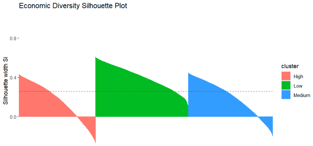
Figure A2.
Cluster plot for economic diversity rendered against a two-dimensional Principal Components Analysis. There is significant overlap between the clusters, suggesting the sizable isolation scores in Table A1.
Figure A2.
Cluster plot for economic diversity rendered against a two-dimensional Principal Components Analysis. There is significant overlap between the clusters, suggesting the sizable isolation scores in Table A1.
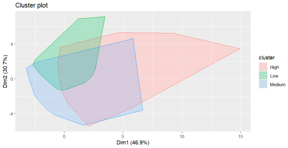
Table A2.
Demographic diversity cluster information for ACS data. The risk profile in this indicator follows the proportion of non-white population [16].
Table A2.
Demographic diversity cluster information for ACS data. The risk profile in this indicator follows the proportion of non-white population [16].
| Metric | Low Risk Cluster | Middle Risk Cluster | High Risk Cluster |
| %White | 88.71% | 64.63% | 23.64% |
| Diversity Index | 0.79 | 0.49 | 0.52 |
| %Women | 50.44% | 50.75% | 50.47% |
| %Children | 20.60% | 20.71% | 23.43% |
| Cluster Size | 30,252 | 28,848 | 21,755 |
| Max Dissimilarity | 1.26 | 0.57 | 1.29 |
| Average Dissimilarity | 0.12 | 0.15 | 0.25 |
| Isolation Ratio | 3.27 | 3.15 | 1.48 |
| Average Silhouette | 0.56 | 0.42 | 0.24 |
| Avg. Global Silhouette: 0.43 | |||
Figure A3.
Silhouette plot of demographic diversity. Overall, demographic diversity shows a weak-to-moderate separation based on an average global silhouette of 0.43 in Table A2. The low risk cluster group is the most isolated of all the groups as evidenced by the height and orientation of the silhouette plot. The low risk category shows a moderate separation based on its silhouette score of 0.56 in Table A2.
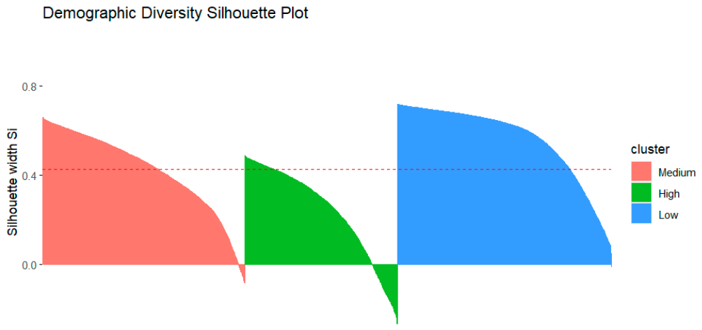
Figure A4.
Cluster plot for demographic diversity rendered against a two-dimensional Principal Components Analysis. The medium group shows a small overlap with the low group, suggesting its lower isolation score in Table A2.
Figure A4.
Cluster plot for demographic diversity rendered against a two-dimensional Principal Components Analysis. The medium group shows a small overlap with the low group, suggesting its lower isolation score in Table A2.
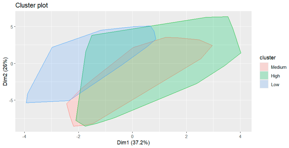
Table A3.
Housing cost cluster information for ACS data. The risk assessment follows the population share under burden, which in this case increases in each dimension [16].
Table A3.
Housing cost cluster information for ACS data. The risk assessment follows the population share under burden, which in this case increases in each dimension [16].
| Metric | Low Risk Cluster | Middle Risk Cluster | High Risk Cluster |
| Mortgage Burden | 5.60% | 6.54% | 6.75% |
| Owner Non-Mortgage Burden | 1.99% | 2.18% | 2.45% |
| Renter Burden | 10.72% | 20.87% | 32.92% |
| Cluster Size | 27,328 | 34,370 | 19,157 |
| Max Dissimilarity | 0.98 | 0.98 | 0.99 |
| Average Dissimilarity | 0.05 | 0.05 | 0.09 |
| Isolation Ratio | 9.65 | 9.63 | 8.21 |
| Average Silhouette | 0.41 | 0.36 | 0.19 |
| Avg. Global Silhouette: 0.34 | |||
Figure A5.
Silhouette plot of housing cost. Overall, housing cost shows a weak separation based on an average global silhouette of 0.34 in Table A3. The low risk cluster group is the most isolated of all the groups as evidenced by the height and orientation of the silhouette plot. The low and medium risk category shows a weak-to-moderate separation based on their silhouette scores in Table A3.
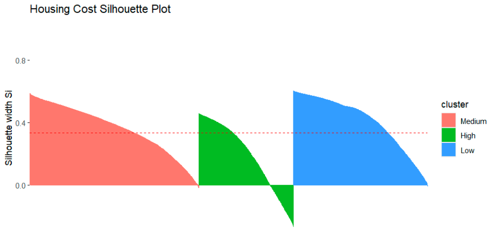
Figure A6.
Cluster plot for housing cost rendered against a two-dimensional Principal Components Analysis. There is a substantive overlap between all of the groups, suggesting the high isolation scores in Table A3.
Figure A6.
Cluster plot for housing cost rendered against a two-dimensional Principal Components Analysis. There is a substantive overlap between all of the groups, suggesting the high isolation scores in Table A3.
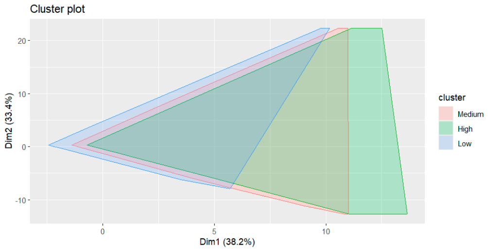
Table A4.
Housing quality cluster information for ACS data. The risk assessment follows the population share under burden, which in this case increases in each dimension [16].
Table A4.
Housing quality cluster information for ACS data. The risk assessment follows the population share under burden, which in this case increases in each dimension [16].
| Metric | Low Risk Cluster | Middle Risk Cluster | High Risk Cluster |
| Housing with Incomplete Kitchens | 0.00% | 1.72% | 7.34% |
| Housing with Incomplete Plumbing | 0.00% | 2.68% | 7.39% |
| Occupied Housing with Incomplete Kitchens | 0.00% | 0.53% | 1.01% |
| Occupied Housing with Incomplete Plumbing | 0.00% | 0.80% | 1.38% |
| Cluster Size | 40,931 | 29,282 | 11,182 |
| Max Dissimilarity | 0.04 | 0.14 | 1.03 |
| Average Dissimilarity | 0.01 | 0.03 | 0.07 |
| Isolation Ratio | 1.21 | 4.32 | 13.92 |
| Average Silhouette | 0.79 | 0.05 | 0.01 |
| Avg. Global Silhouette: 0.41 | |||
Figure A7.
Silhouette plot of housing quality. Overall, housing quality shows a weak-to-moderate separation based on an average global silhouette of 0.41 in Table A4. The low risk cluster group is the most isolated of all the groups as evidenced by the height and orientation of the silhouette plot. The low-risk cluster shows strong separation based on its silhouette score of 0.79 in Table A4.
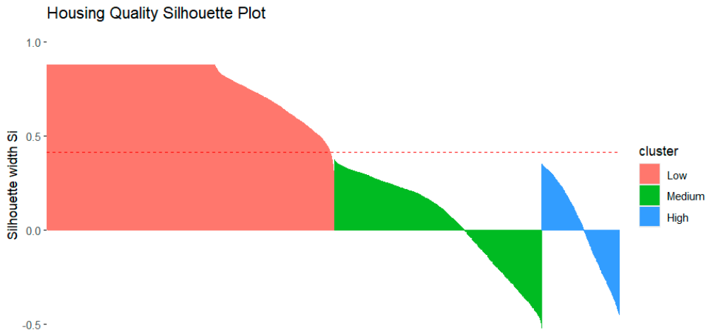
Figure A8.
Cluster plot for housing quality rendered against a two-dimensional Principal Components Analysis. The low cluster is fundamentally isolated from the high cluster, emblematic of its high silhouette score in Table A4.
Figure A8.
Cluster plot for housing quality rendered against a two-dimensional Principal Components Analysis. The low cluster is fundamentally isolated from the high cluster, emblematic of its high silhouette score in Table A4.
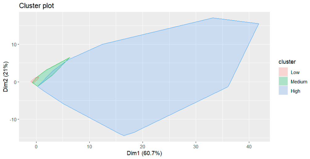
Table A5.
Household factor cluster information for ACS data. The risk assessment follows largest proportions as each metric presents a characteristic emblematic of economic insecurity, and thus housing insecurity challenges [16].
Table A5.
Household factor cluster information for ACS data. The risk assessment follows largest proportions as each metric presents a characteristic emblematic of economic insecurity, and thus housing insecurity challenges [16].
| Metric | Low Risk Cluster | Middle Risk Cluster | High Risk Cluster |
| Households, No Income | 5.84% | 10.77% | 15.90% |
| Households, No Other Income | 29.79% | 36.05% | 44.63% |
| Households, No Investment Income | 26.67% | 33.10% | 39.85% |
| Households, Public Assistance | 2.76% | 5.05% | 8.37% |
| Households, Social Security Insurance | 1.47% | 1.37% | 3.20% |
| Households, No Workers | 6.52% | 11.11% | 17.12% |
| Households, 3+ Workers | 3.51% | 2.82% | 1.51% |
| Households, Workers with No Vehicles | 0.25% | 0.97% | 3.34% |
| Households, No Vehicles | 0.84% | 2.07% | 5.59% |
| Cluster Size | 25,186 | 34,978 | 20,691 |
| Max Dissimilarity | 0.45 | 0.38 | 1.72 |
| Average Dissimilarity | 0.08 | 0.08 | 0.16 |
| Isolation Ratio | 3.85 | 3.33 | 11.70 |
| Average Silhouette | 0.34 | 0.25 | -0.02 |
| Avg. Global Silhouette: 0.21 | |||
Figure A9.
Silhouette plot of household factors. Overall, housing factors shows a weak separation based on an average global silhouette of 0.21 in Table A5. The low risk cluster group is the most isolated of all the groups as evidenced by the height and orientation of the silhouette plot. The low-risk and medium-risk clusters show weak separation based on their silhouette scores in Table A5.
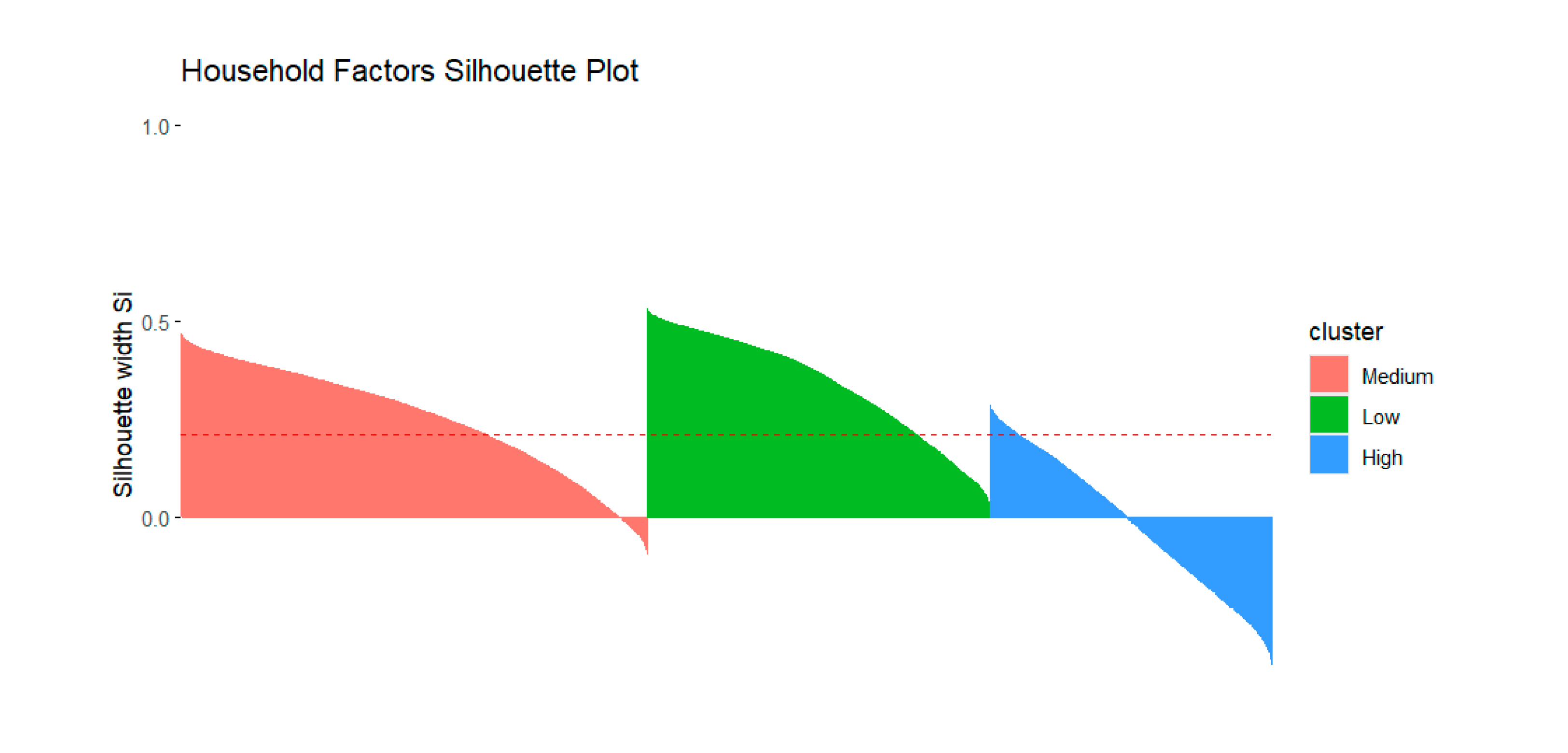
Figure A10.
Cluster plot for household factors rendered against a two-dimensional Principal Components Analysis. The three clusters show sizable intersections, leading to the large isolation score in Table A5 for high risk.
Figure A10.
Cluster plot for household factors rendered against a two-dimensional Principal Components Analysis. The three clusters show sizable intersections, leading to the large isolation score in Table A5 for high risk.
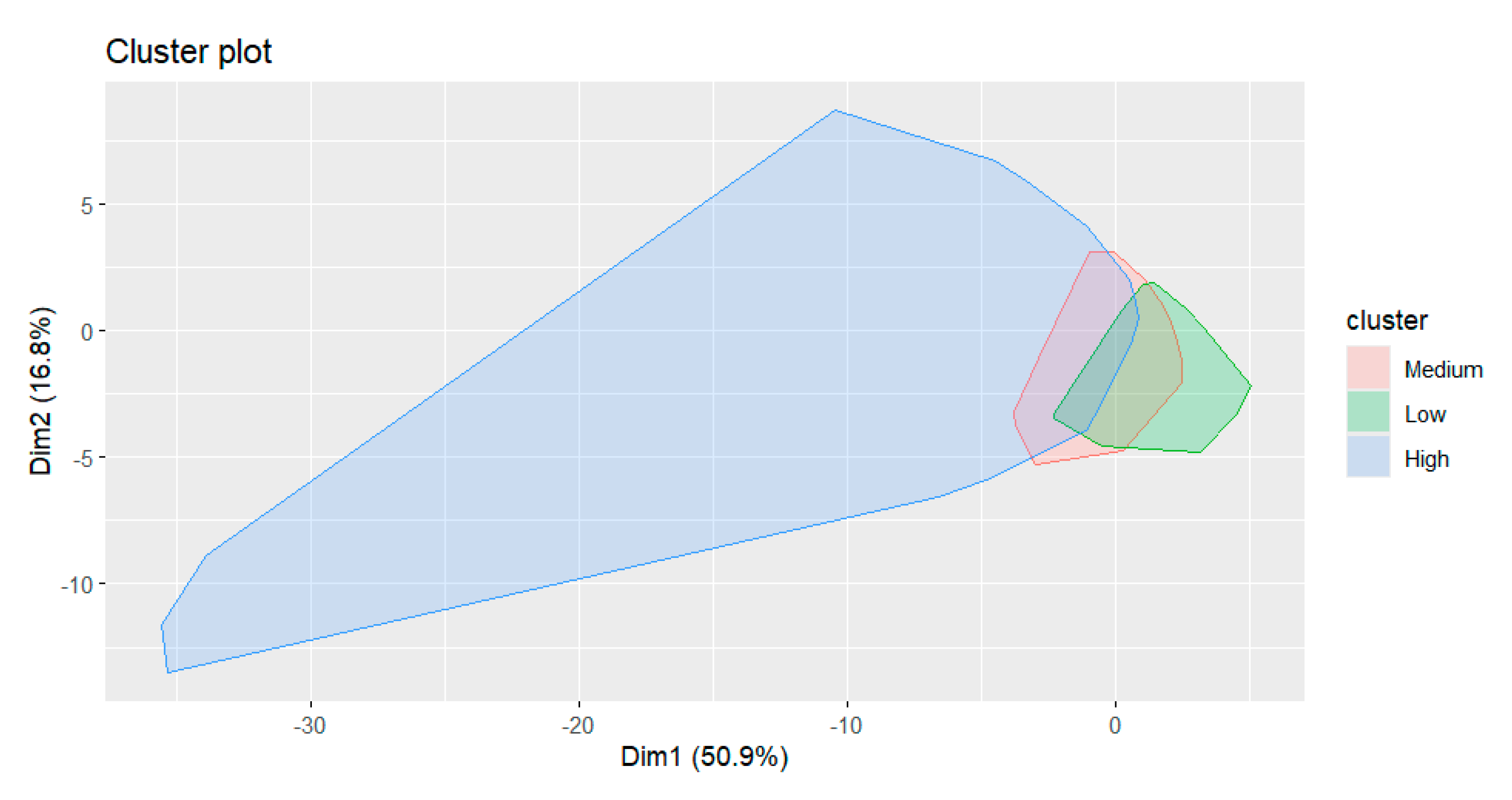
Table A6.
Residential Mobility factor cluster information for ACS data. The risk clusters are organized by amount of mobility, which increases for all three sectors [16].
Table A6.
Residential Mobility factor cluster information for ACS data. The risk clusters are organized by amount of mobility, which increases for all three sectors [16].
| Metric | Low Risk Cluster | Middle Risk Cluster | High Risk Cluster |
| Same House | 97.16% | 90.60% | 80.09% |
| Moved Within County | 1.64% | 5.82% | 13.74% |
| Moved Within State, but Outside County | 0.77% | 2.50% | 3.79% |
| Moved Out of State | 0.44% | 1.07% | 2.38% |
| Cluster Size | 32,949 | 34,978 | 16,302 |
| Max Dissimilarity | 0.10 | 0.23 | 1.26 |
| Average Dissimilarity | 0.03 | 0.05 | 0.12 |
| Isolation Ratio | 1.20 | 2.83 | 9.48 |
| Average Silhouette | 0.59 | 0.21 | 0.03 |
| Avg. Global Silhouette: 0.33 | |||
Figure A11.
Silhouette plot of residential mobility. Overall, residential mobility shows a weak separation based on an average global silhouette of 0.33 in Table A6. The low risk cluster group is the most isolated of all the groups as evidenced by the height and orientation of the silhouette plot. The low-risk clusters shows moderate separation based on its silhouette score in Table A6.
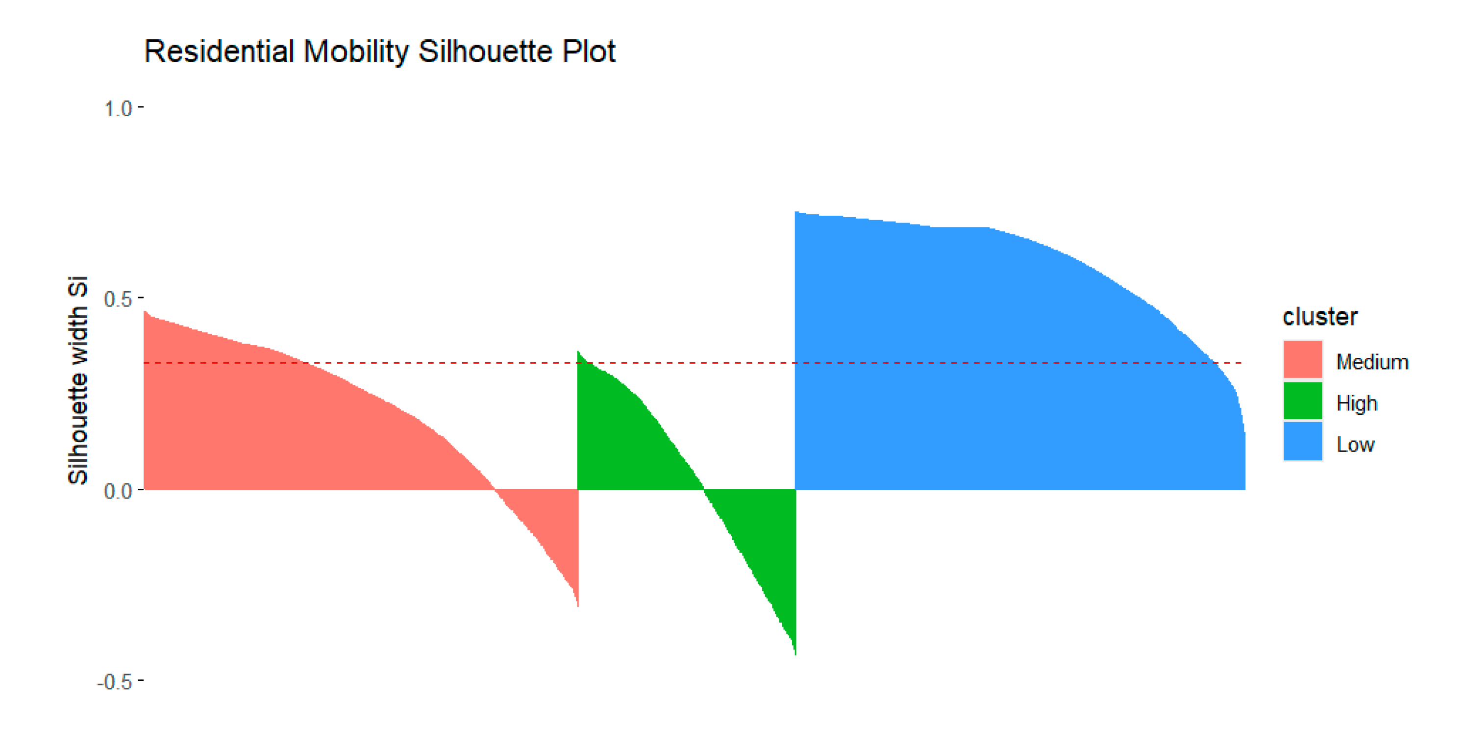
Figure A12.
Cluster plot for residential mobility rendered against a two-dimensional Principal Components Analysis. The low cluster is fundamentally separated from the high cluster, leading to its low isolation score in Table A6.
Figure A12.
Cluster plot for residential mobility rendered against a two-dimensional Principal Components Analysis. The low cluster is fundamentally separated from the high cluster, leading to its low isolation score in Table A6.
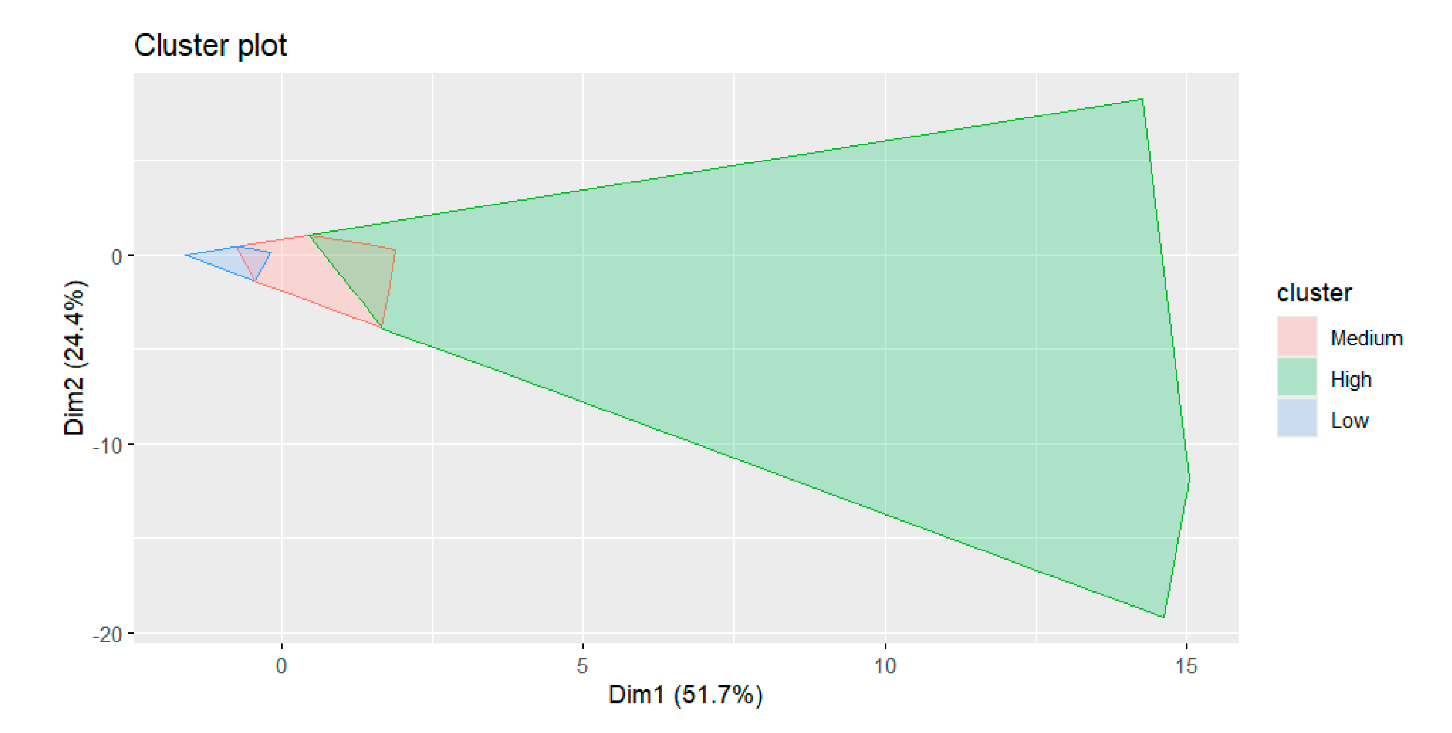
Table A7.
Renter/Owner cluster information for ACS data. The risk clusters are organized by amount of mobility, which increases for all three sectors [16].
Table A7.
Renter/Owner cluster information for ACS data. The risk clusters are organized by amount of mobility, which increases for all three sectors [16].
| Metric | Low Risk Cluster | Middle Risk Cluster | High Risk Cluster |
| Renter/Owner Ratio | 0.37 | 3.21 | 74.84 |
| %Rental Single | 57.09% | 23.58% | 9.91% |
| %Rental 2-4 | 12.12% | 21.78% | 6.33% |
| %Rental 5+ | 22.39% | 54.64% | 83.76% |
| %Rental Mobile Home | 8.41% | 0.00% | 0.00% |
| %Rental Unconvential | 0.00% | 0.00% | 0.00% |
| Cluster Size | 71,117 | 9,298 | 440 |
| Max Dissimilarity | 1.70 | 35.76 | 1593.16 |
| Average Dissimilarity | 0.54 | 2.94 | 69.96 |
| Isolation Ratio | 0.59 | 12.43 | 22.24 |
| Average Silhouette | 0.84 | -0.11 | 0.04 |
| Avg. Global Silhouette: 0.72 | |||
Figure A13.
Silhouette plot of rent characteristics. Overall, rent characteristics shows a strong separation based on an average global silhouette of 0.72 in Table A7. The low risk cluster group is the most isolated of all the groups as evidenced by the height and orientation of the silhouette plot. The low-risk cluster shows strong separation based on its silhouette score in Table A7.
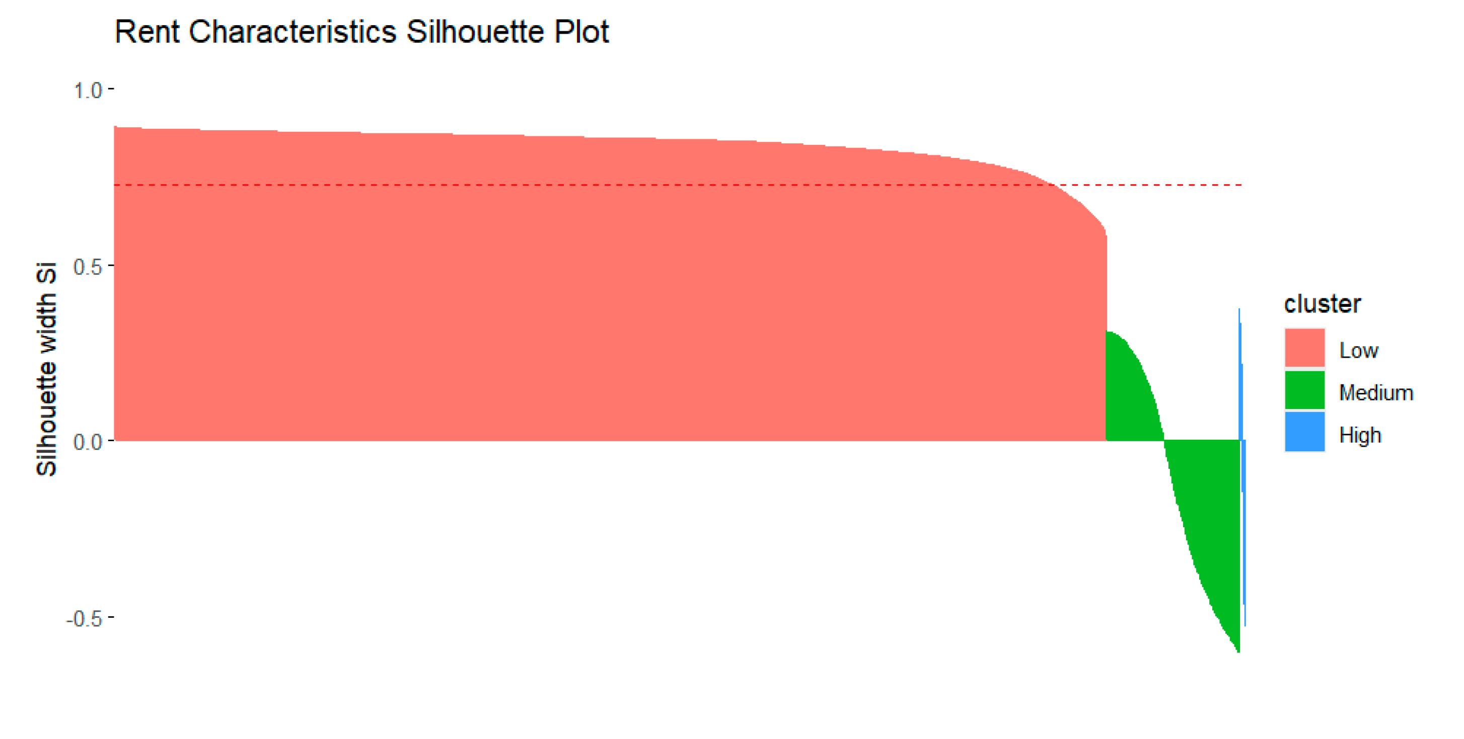
Figure A14.
Cluster plot for rent characteristics rendered against a two-dimensional Principal Components Analysis.
Figure A14.
Cluster plot for rent characteristics rendered against a two-dimensional Principal Components Analysis.
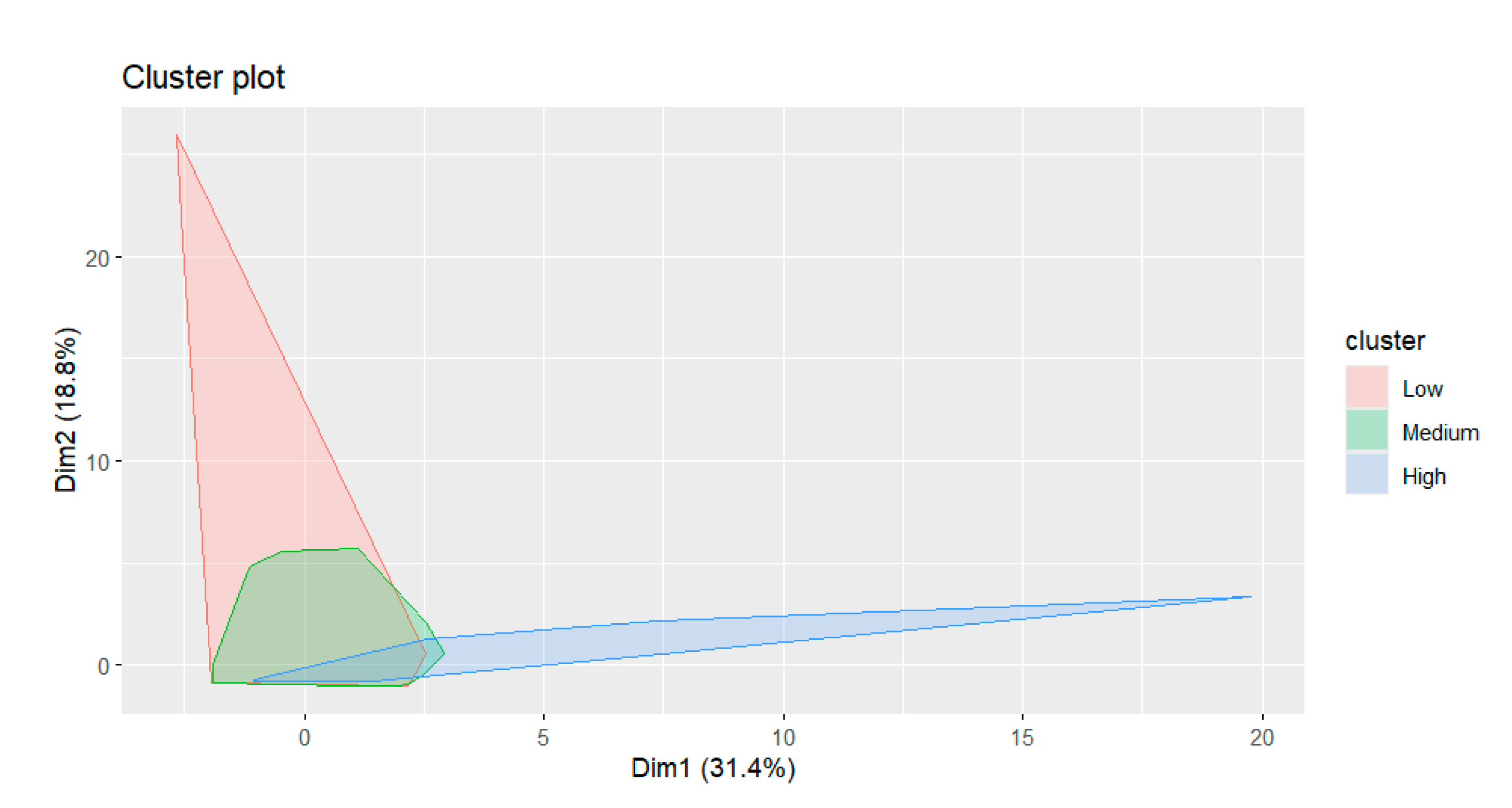
Table A1, Table A2, Table A3, Table A4, Table A5, Table A6 and Table A7 as well as Figure A1, Figure A2, Figure A3, Figure A4, Figure A5, Figure A6, Figure A7, Figure A8, Figure A9, Figure A10, Figure A11, Figure A12, Figure A13 and Figure A14 show a strong trend: the lowest risk cluster had the highest silhouette score, suggesting that these clusters are more rigidly defined, leading to the tallest peaks in the even numbered figures. Similarly, in almost every case, the lowest isolation ratio within the groups occurred for this cluster as well, making it the least overlapping in the odd numbered figures. This is not overly surprising as housing insecurity is a multi-faceted problem, and thus is likely to paint potentially confusing profiles in any one measure [16,25,26]. Because of this, we decided to search for combinations of measures in Section 3.3 and Section 3.4.
Appendix B: Cluster Distribution Across RUCA Codes
Tables B1 through B7 consider the proportion of RUCA coded census tracts that fit into low, medium, and high risk categories across the various dimensions from Section 3.1. These tables support Table 3 in Section 3.2.
Table B1. Economic diversity clusters against RUCA codes. A consistent pattern emerges across the codes: codes 1, 4, and 7 are more evenly distributed, whereas codes 2, 5, and 8 and codes 3, 6, and 9 are weighted toward low and medium risk. As such, the rate of a high risk economic diversity tract is between 2 and 2.5 times as likely in flow centers as it is in areas that outflow to those centers. RUCA Code 10 behaves differently than the rest, where the medium risk is disproportionately largest.
| RUCA Code | Prop L | Prop M | Prop H |
| 1 | 36.92% | 30.48% | 32.60% |
| 2 | 42.44% | 40.76% | 16.80% |
| 3 | 40.40% | 45.03% | 14.57% |
| 4 | 30.25% | 25.48% | 44.27% |
| 5 | 38.16% | 38.03% | 23.81% |
| 6 | 39.04% | 43.69% | 17.27% |
| 7 | 27.93% | 28.35% | 43.72% |
| 8 | 32.89% | 43.26% | 23.85% |
| 9 | 39.88% | 43.15% | 16.96% |
| 10 | 28.73% | 48.18% | 23.09% |
Table B2. Demographic diversity clusters against RUCA codes. A consistent pattern emerges in that flow centers have lower low risk values than their outflow counterparts, and as their size gets smaller, the rate of low risk grows. Similarly, the proportion of high risk spikes in flow centers. RUCA Code 10 behaves much like the outflow tracts.
| RUCA Code | Prop L | Prop M | Prop H |
| 1 | 24.14% | 40.64% | 35.22% |
| 2 | 66.34% | 25.76% | 7.91% |
| 3 | 69.72% | 23.56% | 6.72% |
| 4 | 53.40% | 32.80% | 13.80% |
| 5 | 72.24% | 22.20% | 5.56% |
| 6 | 76.63% | 17.56% | 5.81% |
| 7 | 61.02% | 26.15% | 12.83% |
| 8 | 70.23% | 23.85% | 5.92% |
| 9 | 70.54% | 21.43% | 8.04% |
| 10 | 71.59% | 20.20% | 8.21% |
Table B3. Housing cost clusters against RUCA codes. Housing cost follows a specific pattern: the proportion of low risk is lowest in flow centers and the proportion of high risk spikes in these tracts. The proportions of RUCA codes at different sizes but similar concepts is remarkably consistent. This would suggest that the costs of housing are heavier in flow centers and decrease as tracts become more distant from centers.
| RUCA Code | Prop L | Prop M | Prop H |
| 1 | 27.31% | 45.68% | 27.00% |
| 2 | 52.08% | 31.79% | 16.12% |
| 3 | 56.37% | 30.72% | 12.91% |
| 4 | 28.03% | 47.62% | 24.35% |
| 5 | 56.46% | 31.26% | 12.29% |
| 6 | 58.93% | 30.33% | 10.74% |
| 7 | 28.21% | 48.73% | 23.06% |
| 8 | 61.35% | 27.14% | 11.51% |
| 9 | 59.52% | 28.87% | 11.61% |
| 10 | 53.38% | 33.22% | 13.40% |
Table B4. Housing quality clusters against RUCA codes. A pattern emerges in the table where other than in RUCA code 1, the proportion of medium risk tracts is largely the same. The common pattern that we have seen before shows again. Flow centers have the highest rate of low risk, and that declines both by outflow group and by population size. Conversely, the high risk proportion climbs as tracts become further from the population center. RUCA Code 10 is a relative culmination of this pattern.
| RUCA Code | Prop L | Prop M | Prop H |
| 1 | 58.48% | 33.09% | 8.44% |
| 2 | 43.19% | 41.22% | 15.59% |
| 3 | 29.84% | 44.76% | 25.39% |
| 4 | 38.36% | 42.89% | 18.74% |
| 5 | 22.87% | 46.28% | 30.85% |
| 6 | 21.34% | 46.15% | 32.51% |
| 7 | 31.85% | 42.69% | 25.46% |
| 8 | 14.80% | 41.94% | 43.26% |
| 9 | 15.48% | 45.83% | 38.69% |
| 10 | 17.71% | 43.51% | 38.78% |
Table B5. Household factors clusters against RUCA codes. These proportions show a different pattern than in prior risk dimensions. As tracts progress down the code designation, the rate of low risk tracts generally declines. The rate of high risk tracks behaves in the hypothesized groups: the proportion of highest risk is in the flow centers and ascends as those centers gets smaller. Unlike other dimensions, the lower outflow group has a higher risk than the larger one.
| RUCA Code | Prop L | Prop M | Prop H |
| 1 | 36.08% | 38.21% | 25.71% |
| 2 | 36.34% | 52.62% | 11.04% |
| 3 | 23.21% | 60.73% | 16.06% |
| 4 | 13.69% | 46.69% | 39.63% |
| 5 | 13.95% | 67.71% | 18.34% |
| 6 | 11.47% | 64.44% | 24.09% |
| 7 | 7.21% | 42.83% | 49.97% |
| 8 | 8.22% | 65.46% | 26.32% |
| 9 | 6.85% | 61.01% | 32.14% |
| 10 | 11.98% | 55.72% | 32.29% |
Table B6. Residential mobility clusters against RUCA codes. The consistent pattern of flow proportion shows up here as well. The highest risk tracts are in the flow centers with declining risk as that flow rate declines. Similarly, the low risk tracts behave opposite of that phenomenon. The most urban centers have the highest low risk rate. As the flow centers shrink, the proportion is traded to medium risk.
| RUCA Code | Prop L | Prop M | Prop H |
| 1 | 38.29% | 38.21% | 23.50% |
| 2 | 52.52% | 37.87% | 9.61% |
| 3 | 56.81% | 37.35% | 5.85% |
| 4 | 28.55% | 44.22% | 27.22% |
| 5 | 52.74% | 38.57% | 8.70% |
| 6 | 56.60% | 38.03% | 5.37% |
| 7 | 26.84% | 50.72% | 22.44% |
| 8 | 57.24% | 35.53% | 7.24% |
| 9 | 54.17% | 41.96% | 3.87% |
| 10 | 47.72% | 42.88% | 9.40% |
Table B7. Renter characteristics clusters against RUCA codes. There is overall a low risk of housing insecurity on this factor group, with the highest and medium risk tracts existing in flow centers. There is the common pattern of flow and outflow, but the sheer number of low risk tracts make it harder to see practically. The pattern is most easily seen amongst the medium and high risk tracts.
| RUCA Code | Prop L | Prop M | Prop H |
| 1 | 83.18% | 16.06% | 0.76% |
| 2 | 99.36% | 0.63% | 0.02% |
| 3 | 99.74% | 0.26% | 0.00% |
| 4 | 93.13% | 6.65% | 0.22% |
| 5 | 99.87% | 0.13% | 0.00% |
| 6 | 100.00% | 0.00% | 0.00% |
| 7 | 97.53% | 2.20% | 0.27% |
| 8 | 99.67% | 0.33% | 0.00% |
| 9 | 99.70% | 0.30% | 0.00% |
| 10 | 99.53% | 0.42% | 0.05% |
A basic pattern emerges throughout most of Tables B1-B7. RUCA codes seem to predict a general pattern in the rate data: as we move further from a flow center, something happens to the rate. Largely, the size of the flow center does not change this, though it may spike or mute the individual rate as the case may dictate.
Appendix C: Association Rules Output
An association rules mining procedure was run on subsets of the dataset, separated by RUCA codes. The resulting association rules are shown in Tables C1-C10. These tables support Table 6 in Section 3.4.
Table C1. Association rules between high risk tracts within the different factors for only RUCA code 1, sorted by lift. A total of 23 combinations have a confidence of at least 30%. These rules are not necessarily symmetric, however some of them are.
| lhs | rhs | Support | Confidence | coverage | Lift | Count |
| {ROC=H} | {HHFC=H} | 0.004995 | 0.654028436 | 0.0076376 | 2.543966 | 276 |
| {ROC=H} | {RMC=H} | 0.003656 | 0.478672986 | 0.0076376 | 2.036664 | 202 |
| {ROC=H} | {EDC=H} | 0.00485 | 0.63507109 | 0.0076376 | 1.947798 | 268 |
| {HHFC=H} | {HCC=H} | 0.13469 | 0.523900035 | 0.2570901 | 1.940021 | 7442 |
| {HCC=H} | {HHFC=H} | 0.13469 | 0.498760137 | 0.2700487 | 1.940021 | 7442 |
| {HQC=H} | {HHFC=H} | 0.041681 | 0.494099979 | 0.0843574 | 1.921894 | 2303 |
| {ROC=H} | {DDC=H} | 0.004742 | 0.620853081 | 0.0076376 | 1.762614 | 262 |
| {HQC=H} | {DDC=H} | 0.051617 | 0.611885861 | 0.0843574 | 1.737156 | 2852 |
| {HQC=H} | {EDC=H} | 0.045862 | 0.543660159 | 0.0843574 | 1.667436 | 2534 |
| {ROC=H} | {HCC=H} | 0.003258 | 0.426540284 | 0.0076376 | 1.579494 | 180 |
| {HHFC=H} | {EDC=H} | 0.126599 | 0.492432242 | 0.2570901 | 1.510317 | 6995 |
| {EDC=H} | {HHFC=H} | 0.126599 | 0.388287538 | 0.3260456 | 1.510317 | 6995 |
| {HHFC=H} | {RMC=H} | 0.086348 | 0.335867652 | 0.2570901 | 1.429054 | 4771 |
| {RMC=H} | {HHFC=H} | 0.086348 | 0.367395657 | 0.235028 | 1.429054 | 4771 |
| {EDC=H} | {DDC=H} | 0.150073 | 0.460283097 | 0.3260456 | 1.306753 | 8292 |
| {DDC=H} | {EDC=H} | 0.150073 | 0.426061042 | 0.3522343 | 1.306753 | 8292 |
| {RMC=H} | {HCC=H} | 0.080412 | 0.342137687 | 0.235028 | 1.266948 | 4443 |
| {HCC=H} | {EDC=H} | 0.110039 | 0.407479391 | 0.2700487 | 1.249762 | 6080 |
| {EDC=H} | {HCC=H} | 0.110039 | 0.337496531 | 0.3260456 | 1.249762 | 6080 |
| {HQC=H} | {HCC=H} | 0.027021 | 0.320317528 | 0.0843574 | 1.186147 | 1493 |
| {RMC=H} | {EDC=H} | 0.086077 | 0.366240567 | 0.235028 | 1.12328 | 4756 |
| {HHFC=H} | {DDC=H} | 0.085642 | 0.33312214 | 0.2570901 | 0.94574 | 4732 |
| {RMC=H} | {DDC=H} | 0.073752 | 0.313799476 | 0.235028 | 0.890883 | 4075 |
Table C2. Association rules between high risk tracts within the different factors for only RUCA code 2, sorted by lift. A total of 2 combinations have a confidence of at least 30%.
| lhs | rhs | Support | confidence | coverage | Lift | Count |
| {HHFC=H} | {HQC=H} | 0.034651107 | 0.3139159 | 0.110383 | 2.013954 | 291 |
| {DDC=H} | {EDC=H} | 0.024053346 | 0.3042169 | 0.079066 | 1.81064 | 202 |
Table C3. Association rules between high risk tracts within the different factors for only RUCA code 3, sorted by lift. A total of 4 combinations have a confidence of at least 30%.
| lhs | rhs | support | confidence | coverage | Lift | Count |
| {HCC=H} | {HHFC=H} | 0.042757 | 0.331081081 | 0.1291449 | 2.062059 | 49 |
| {DDC=H} | {HQC=H} | 0.030541 | 0.454545455 | 0.0671902 | 1.790066 | 35 |
| {HHFC=H} | {HQC=H} | 0.0637 | 0.39673913 | 0.1605585 | 1.562416 | 73 |
| {EDC=H} | {HQC=H} | 0.057592 | 0.395209581 | 0.1457243 | 1.556392 | 66 |
Table C4. Association rules between high risk tracts within the different factors for only RUCA code 4, sorted by lift. A total of 17 combinations have a confidence of at least 30%. These rules are not necessarily symmetric, however some of them are.
| lhs | rhs | support | confidence | coverage | Lift | Count |
| {ROC=H} | {RMC=H} | 0.001744 | 0.8 | 0.0021796 | 2.938671 | 8 |
| {DDC=H} | {HQC=H} | 0.053618 | 0.388625592 | 0.1379686 | 2.073272 | 246 |
| {HCC=H} | {HHFC=H} | 0.152354 | 0.625783348 | 0.2434612 | 1.57926 | 699 |
| {HHFC=H} | {HCC=H} | 0.152354 | 0.384488449 | 0.3962511 | 1.57926 | 699 |
| {ROC=H} | {EDC=H} | 0.001308 | 0.6 | 0.0021796 | 1.355391 | 6 |
| {HHFC=H} | {EDC=H} | 0.226678 | 0.572057206 | 0.3962511 | 1.292269 | 1040 |
| {EDC=H} | {HHFC=H} | 0.226678 | 0.512063023 | 0.4426765 | 1.292269 | 1040 |
| {HQC=H} | {HHFC=H} | 0.095902 | 0.511627907 | 0.1874455 | 1.291171 | 440 |
| {HQC=H} | {EDC=H} | 0.106364 | 0.56744186 | 0.1874455 | 1.281843 | 488 |
| {HCC=H} | {EDC=H} | 0.13143 | 0.539838854 | 0.2434612 | 1.219488 | 603 |
| {DDC=H} | {EDC=H} | 0.070183 | 0.508688784 | 0.1379686 | 1.149121 | 322 |
| {RMC=H} | {EDC=H} | 0.138405 | 0.508406725 | 0.2722319 | 1.148484 | 635 |
| {EDC=H} | {RMC=H} | 0.138405 | 0.312653865 | 0.4426765 | 1.148484 | 635 |
| {RMC=H} | {HHFC=H} | 0.120968 | 0.444355484 | 0.2722319 | 1.121399 | 555 |
| {HHFC=H} | {RMC=H} | 0.120968 | 0.305280528 | 0.3962511 | 1.121399 | 555 |
| {HCC=H} | {RMC=H} | 0.073888 | 0.303491495 | 0.2434612 | 1.114827 | 339 |
| {DDC=H} | {HHFC=H} | 0.045118 | 0.327014218 | 0.1379686 | 0.82527 | 207 |
Table C5. Association rules between high risk tracts within the different factors for only RUCA code 5, sorted by lift. A total of 9 combinations have a confidence of at least 30%.
| lhs | rhs | support | confidence | coverage | Lift | Count |
| {HCC=H} | {HHFC=H} | 0.040359 | 0.328467153 | 0.12287 | 1.790909 | 90 |
| {DDC=H} | {HQC=H} | 0.029596 | 0.532258065 | 0.0556054 | 1.725197 | 66 |
| {HHFC=H} | {EDC=H} | 0.069507 | 0.378973105 | 0.1834081 | 1.591544 | 155 |
| {DDC=H} | {EDC=H} | 0.019731 | 0.35483871 | 0.0556054 | 1.490189 | 44 |
| {HHFC=H} | {HQC=H} | 0.078924 | 0.430317848 | 0.1834081 | 1.39478 | 176 |
| {RMC=H} | {EDC=H} | 0.028251 | 0.324742268 | 0.0869955 | 1.363795 | 63 |
| {HCC=H} | {EDC=H} | 0.039013 | 0.317518248 | 0.12287 | 1.333457 | 87 |
| {EDC=H} | {HQC=H} | 0.086099 | 0.361581921 | 0.2381166 | 1.171988 | 192 |
| {RMC=H} | {HQC=H} | 0.026457 | 0.304123711 | 0.0869955 | 0.98575 | 59 |
Table C6. Association rules between high risk tracts within the different factors for only RUCA code 6, sorted by lift. A total of 12 combinations have a confidence of at least 30%. These rules are not necessarily symmetric, however some of them are.
| lhs | rhs | support | confidence | coverage | Lift | Count |
| {DDC=H} | {EDC=H} | 0.021771 | 0.375 | 0.0580552 | 2.171218 | 15 |
| {HCC=H} | {EDC=H} | 0.037736 | 0.351351351 | 0.107402 | 2.034295 | 26 |
| {HHFC=H} | {EDC=H} | 0.075472 | 0.313253012 | 0.2409289 | 1.813709 | 52 |
| {EDC=H} | {HHFC=H} | 0.075472 | 0.43697479 | 0.1727141 | 1.813709 | 52 |
| {HCC=H} | {HHFC=H} | 0.046444 | 0.432432432 | 0.107402 | 1.794855 | 32 |
| {DDC=H} | {HQC=H} | 0.033382 | 0.575 | 0.0580552 | 1.768638 | 23 |
| {DDC=H} | {HHFC=H} | 0.024673 | 0.425 | 0.0580552 | 1.764006 | 17 |
| {RMC=H} | {HHFC=H} | 0.017417 | 0.324324324 | 0.053701 | 1.346141 | 12 |
| {HHFC=H} | {HQC=H} | 0.103048 | 0.427710843 | 0.2409289 | 1.315593 | 71 |
| {HQC=H} | {HHFC=H} | 0.103048 | 0.316964286 | 0.3251089 | 1.315593 | 71 |
| {EDC=H} | {HQC=H} | 0.060958 | 0.352941176 | 0.1727141 | 1.085609 | 42 |
| {RMC=H} | {HQC=H} | 0.017417 | 0.324324324 | 0.053701 | 0.997587 | 12 |
Table C7. Association rules between high risk tracts within the different factors for only RUCA code 7, sorted by lift. A total of 13 combinations have a confidence of at least 30%. These rules are not necessarily symmetric, however some of them are.
| lhs | rhs | support | confidence | coverage | Lift | Count |
| {ROC=H} | {RMC=H} | 0.002745 | 1 | 0.0027454 | 4.455657 | 4 |
| {DDC=H} | {HQC=H} | 0.07138 | 0.556149733 | 0.1283459 | 2.184124 | 104 |
| {HCC=H} | {HHFC=H} | 0.174331 | 0.755952381 | 0.2306108 | 1.512943 | 254 |
| {HHFC=H} | {HCC=H} | 0.174331 | 0.348901099 | 0.4996568 | 1.512943 | 254 |
| {RMC=H} | {EDC=H} | 0.118051 | 0.525993884 | 0.2244338 | 1.203097 | 172 |
| {EDC=H} | {HHFC=H} | 0.26081 | 0.596546311 | 0.4371997 | 1.193912 | 380 |
| {HHFC=H} | {EDC=H} | 0.26081 | 0.521978022 | 0.4996568 | 1.193912 | 380 |
| {HCC=H} | {EDC=H} | 0.115992 | 0.50297619 | 0.2306108 | 1.150449 | 169 |
| {HQC=H} | {EDC=H} | 0.126973 | 0.498652291 | 0.2546328 | 1.140559 | 185 |
| {DDC=H} | {EDC=H} | 0.060398 | 0.470588235 | 0.1283459 | 1.076369 | 88 |
| {RMC=H} | {HHFC=H} | 0.118737 | 0.529051988 | 0.2244338 | 1.058831 | 173 |
| {HQC=H} | {HHFC=H} | 0.123542 | 0.485175202 | 0.2546328 | 0.971017 | 180 |
| {DDC=H} | {HHFC=H} | 0.059025 | 0.459893048 | 0.1283459 | 0.920418 | 86 |
Table C8. Association rules between high risk tracts within the different factors for only RUCA code 8, sorted by lift. A total of 12 combinations have a confidence of at least 30%. These rules are not necessarily symmetric, however some of them are.
| lhs | rhs | support | confidence | coverage | Lift | Count |
| {HCC=H} | {HHFC=H} | 0.055921 | 0.485714286 | 0.1151316 | 1.845714 | 34 |
| {DDC=H} | {EDC=H} | 0.024671 | 0.416666667 | 0.0592105 | 1.747126 | 15 |
| {HCC=H} | {EDC=H} | 0.042763 | 0.371428571 | 0.1151316 | 1.557438 | 26 |
| {DDC=H} | {HHFC=H} | 0.023026 | 0.388888889 | 0.0592105 | 1.477778 | 14 |
| {EDC=H} | {HHFC=H} | 0.092105 | 0.386206897 | 0.2384868 | 1.467586 | 56 |
| {HHFC=H} | {EDC=H} | 0.092105 | 0.35 | 0.2631579 | 1.467586 | 56 |
| {RMC=H} | {EDC=H} | 0.024671 | 0.340909091 | 0.0723684 | 1.429467 | 15 |
| {DDC=H} | {HQC=H} | 0.036184 | 0.611111111 | 0.0592105 | 1.412759 | 22 |
| {RMC=H} | {HHFC=H} | 0.023026 | 0.318181818 | 0.0723684 | 1.209091 | 14 |
| {RMC=H} | {HQC=H} | 0.034539 | 0.477272727 | 0.0723684 | 1.103353 | 21 |
| {HHFC=H} | {HQC=H} | 0.116776 | 0.44375 | 0.2631579 | 1.025856 | 71 |
| {EDC=H} | {HQC=H} | 0.098684 | 0.413793103 | 0.2384868 | 0.956602 | 60 |
Table C9. Association rules between high risk tracts within the different factors for only RUCA code 9, sorted by lift. A total of 9 combinations have a confidence of at least 30%. These rules are not necessarily symmetric, however some of them are.
| lhs | rhs | support | confidence | coverage | Lift | Count |
| {HCC=H} | {HHFC=H} | 0.077381 | 0.666666667 | 0.1160714 | 2.074074 | 26 |
| {DDC=H} | {HHFC=H} | 0.047619 | 0.592592593 | 0.0803571 | 1.843621 | 16 |
| {DDC=H} | {HQC=H} | 0.044643 | 0.555555556 | 0.0803571 | 1.435897 | 15 |
| {RMC=H} | {HHFC=H} | 0.014881 | 0.384615385 | 0.0386905 | 1.196581 | 5 |
| {HHFC=H} | {HQC=H} | 0.139881 | 0.435185185 | 0.3214286 | 1.124786 | 47 |
| {HQC=H} | {HHFC=H} | 0.139881 | 0.361538462 | 0.3869048 | 1.124786 | 47 |
| {EDC=H} | {HHFC=H} | 0.059524 | 0.350877193 | 0.1696429 | 1.091618 | 20 |
| {EDC=H} | {HQC=H} | 0.065476 | 0.385964912 | 0.1696429 | 0.997571 | 22 |
| {HCC=H} | {HQC=H} | 0.03869 | 0.333333333 | 0.1160714 | 0.861538 | 13 |
Table C10. Association rules between high risk tracts within the different factors for only RUCA code 10, sorted by lift. A total of 13 combinations have a confidence of at least 30%. These rules are not necessarily symmetric, however some of them are.
| lhs | rhs | support | confidence | coverage | Lift | Count |
| {HCC=H} | {HHFC=H} | 0.075772 | 0.565533981 | 0.1339837 | 1.751276 | 466 |
| {DDC=H} | {EDC=H} | 0.032846 | 0.4 | 0.0821138 | 1.732394 | 202 |
| {DDC=H} | {HQC=H} | 0.04813 | 0.586138614 | 0.0821138 | 1.511427 | 296 |
| {EDC=H} | {HHFC=H} | 0.108455 | 0.46971831 | 0.2308943 | 1.454566 | 667 |
| {HHFC=H} | {EDC=H} | 0.108455 | 0.335850957 | 0.3229268 | 1.454566 | 667 |
| {HCC=H} | {EDC=H} | 0.044553 | 0.332524272 | 0.1339837 | 1.440158 | 274 |
| {RMC=H} | {HHFC=H} | 0.034309 | 0.365051903 | 0.0939837 | 1.130448 | 211 |
| {EDC=H} | {HQC=H} | 0.098862 | 0.428169014 | 0.2308943 | 1.104084 | 608 |
| {HHFC=H} | {HQC=H} | 0.137236 | 0.424974824 | 0.3229268 | 1.095847 | 844 |
| {HQC=H} | {HHFC=H} | 0.137236 | 0.353878407 | 0.3878049 | 1.095847 | 844 |
| {DDC=H} | {HHFC=H} | 0.027642 | 0.336633663 | 0.0821138 | 1.042446 | 170 |
| {RMC=H} | {HQC=H} | 0.036423 | 0.387543253 | 0.0939837 | 0.999325 | 224 |
| {HCC=H} | {HQC=H} | 0.040488 | 0.302184466 | 0.1339837 | 0.779218 | 249 |
References
- Dewey, R. The rural-urban continuum: real but relatively unimportant. Am. J. Sociol. 1960, 66(1), 60–66. [Google Scholar] [CrossRef]
- Rajagopalan, C. The rural-urban continuum: a critical evaluation. Sociol. Bull. 1961, 10(1), 61–74. [Google Scholar] [CrossRef]
- Bell, M. The fruit of difference: the rural-urban continuum as a system of identity. Rural Sociol. 1992, 57(1), 65–82. [Google Scholar] [CrossRef]
- Golding, S.A.; Winkler, R.L. Tracking urbanization and exurbs: migration across the rural-urban continuum, 1990-2016. Popul. Res. Policy Rev. 2020, 39(5), 835–859. [Google Scholar] [CrossRef]
- Lichter, D.T.; Johnson, K.F. Depopulation, deaths, diversity, and deprivation: the 4 Ds of rural population change. Russell Sage Found. J. Soc. Sci. 2025, 11(2), 88–114. [Google Scholar] [CrossRef]
- Powell, R.J.; Clark, J.T.; Dube, M.P. Partisan gerrymandering, clustering, or both? A new approach to a persistent question. Elect. Law J. Rules Politics Policy 2020, 19(1), 79–100. [Google Scholar] [CrossRef]
- Mettler, S.; Brown, T.E. The growing rural-urban political divide and democratic vulnerability. Ann. Am. Acad. Political Soc. Sci. 2022, 699(1), 130–142. [Google Scholar] [CrossRef]
- Brown, T.E.; Mettler, S. Sequential polarization: the development of the rural-urban political divide, 1976-2020. Perspect. Politics 2024, 22(3), 630–658. [Google Scholar] [CrossRef]
- Kelly, P.; Lobao, L. The social bases of rural-urban political divides: social status, work, and sociocultural beliefs. Rural Sociol. 2019, 84(4), 669–705. [Google Scholar] [CrossRef]
- Lobao, L.; Kelly, P. Local governments across the rural-urban continuum: findings from a recent national county government study. State Local Gov. Rev. 2019, 51(4), 223–232. [Google Scholar] [CrossRef]
- Brown, T.E.; Jauregui, G.P.; Mettler, S.; Rivera, M. A rural-urban political divide among whom? Race, ethnicity, and political behavior across place. Politics Groups Identities 2025, 13(1), 229–242. [Google Scholar] [CrossRef]
- Tsvetkova, A.; Partridge, M.; Betz, M. Entrepreneurial and employment responses to economic conditions across the rural-urban continuum. Ann. Am. Acad. Political Soc. Sci. 2017, 672(1), 83–102. [Google Scholar] [CrossRef]
- Auzina-Emsina, A.; Ozolina, V. Modelling impact of urban-rural income convergence in the EU. Res. Rural Dev. 2019, 2. [Google Scholar] [CrossRef]
- Walton, S.; Lobao, L.; Dube, M.P. Jail incarceration across the US: the role of the local state and place-based punishment vulnerability. Punishm. Soc. 2026, 28(2), 409–429. [Google Scholar] [CrossRef]
- Eason, J.M.; Zucker, D.; Wildeman, C. Mass imprisonment across the rural-urban interface. Ann. Am. Acad. Political Soc. Sci. 2017, 672(1), 202–216. [Google Scholar] [CrossRef]
- Garcia, S. Rurality and robustness: rural communities and housing insecurity risk. Masters Thesis, University of Maine, Orono, ME, USA, 2024. [Google Scholar]
- Lichter, D.T.; Brown, D.L. Rural America in an urban society: changing spatial and social boundaries. Annu. Rev. Sociol. 2011, 37(1), 565–592. [Google Scholar] [CrossRef]
- United States Department of Agriculture. Rural-Urban Commuting Area Codes - Descriptions and Maps. Available online: https://www.ers.usda.gov/data-products/rural-urban-commuting-area-codes/descriptions-and-maps.
- Onega, T.; Weiss, J.E.; Alford-Teaster, J.; Goodrich, M.; Eliassen, M.S.; Kim, S.J. Concordance of rural-urban self-identity and ZIP code-derived rural-urban commuting area (RUCA) designation. J. Rural Health 2020, 36(2), 274–280. [Google Scholar] [CrossRef]
- Fowler, C.S.; Cromartie, J. The role of data sample uncertainty in delineations of core based statistical areas and rural urban commuting areas. Spat. Demogr. 2023, 11(2), 6. [Google Scholar] [CrossRef]
- Swope, C.B.; Hernandez, D. Housing as a determinant of health equity: a conceptual model. Soc. Sci. Med. 2019, 243(1), 112571. [Google Scholar] [CrossRef]
- Coleman-Jensen, A.; Steffen, B.; Whitley, S. Food insecurity and housing insecurity. In Rural Poverty in the United States; Tickamyer, A.R., Sherman, J. Warlick, J., Eds.; Columbia University Press: New York City, 2017; pp. 257–298. [Google Scholar]
- Smith, M.; Byrne, T.; Montgomery, A.E. Examining the relationships between exposure to homelessness and attitudes toward homelessness among low- and moderate-income people. J. Soc. Distress Homelessness 2024, 33(2), 356–367. [Google Scholar] [CrossRef]
- Fitchen, J.M. On the edge of homelessness: rural poverty and housing insecurity. Rural Sociol. 1992, 57(2), 173–193. [Google Scholar] [CrossRef]
- Gleason, K.D.; Dube, M.P.; Bernier, E.; Martin, J. Using geographic information systems to assess community-level vulnerability to housing insecurity in rural areas. J. Community Psychol. 2022, 50(4), 1993–2012. [Google Scholar] [CrossRef]
- Gleason, K.D.; Dube, M.P.; Martin, J.; Bernier, E.; Gipson, J. Rural housing insecurity: a case study comparison across four rural areas in Maine. J. Ethnogr. Qual. Res. 2023, 17(1), 39. [Google Scholar]
- Gleason, K.D.; Martin, J.; Bernier, E. Community narratives on rural homelessness: tales of terror and tales of compassion. J. Prev. Interv. Community 2024, 52(1), 143–172. [Google Scholar] [CrossRef]
- Sherman, J. “Please don’t take this”: rural gentrification, symbolic capital, and housing insecurity. Soc. Probl. 2023, 70(2), 491–510. [Google Scholar] [CrossRef]
- Ndaba, Z.; Mncayi-Makhanya, P.; Dunga, S.H. Determinants of housing insecurity in urban and rural South Africa. Cogent Soc. Sci. 2025, 11(1), 2568736. [Google Scholar] [CrossRef]
- Montanez, M. Nowhere else to go: housing insecurity in a Hispanic-majority rural county during the COVID-19 pandemic. Rural Sociol. 2024, 89(1), 106–129. [Google Scholar] [CrossRef]
- Smith, M.N.; Winkler, R.L.; Johnson, K.M. How migration impacts rural America. Rural Popul. Res. Netw. 2016, 3. [Google Scholar]
- Van Sant, L.; Shelton, T.; Kay, K. Connecting country and city: the multiple geographies of real property in ownership in the US. Geogr. Compass 2023, 17, e12677. [Google Scholar] [CrossRef]
- Tieken, M.C. Rural poverty and rural schools. Bloomsbury Handb. Rural Educ. U. S. 2022, 62–71. [Google Scholar]
- Rousseeuw, P.J. Silhouettes: a graphical aid to the interpretation and validation of cluster analysis. J. Comput. Appl. Math. 1987, 20(1), 53–65. [Google Scholar] [CrossRef]
- Agrawal, R.; Imielinski, T.; Swami, A. Mining association rules between sets of items in large databases. In Proceedings of the 1993 ACM SIGMOD International Conference on Management of Data, 1993; pp. 207–216. [Google Scholar]
- Eason, J.M. Big House on the Prairie: Rise of the Rural Ghetto and Prison Proliferation; University of Chicago Press: Chicago, 2017. [Google Scholar]
- Guo, C.; Zhou, W.; Jing, C.; Zhaxi, D. Mapping and measuring urban-rural inequalities in accessibility to social infrastructures. Geogr. Sustain. 2024, 5(1), 41–51. [Google Scholar] [CrossRef]
- Slack, T.; Thiede, B.C.; Jensen, L. Race, residence, and underemployment: fifty years in comparative perspective, 1968–2017. Rural Sociol. 2020, 85(2), 275–315. [Google Scholar] [CrossRef]
- Lee, B.A.; Sharp, G. Ethnoracial diversity across the rural-urban continuum. Ann. Am. Acad. Political Soc. Sci. 2017, 672(1), 26–45. [Google Scholar] [CrossRef]
- Hulchanski, J.D. Private rental housing in Canada’s four largest metropolitan areas: Trends and prospects. Cities Afford. Hous. 2021, 274–288. [Google Scholar]
- De Bruyne, K.; Van Hove, J. Explaining the spatial variation in housing prices: an economic geography approach. Appl. Econ. 2013, 45(13), 1673–1689. [Google Scholar] [CrossRef]
- Dong, H. The impact of income inequality on rental affordability: an empirical study in large American metropolitan areas. Urban Stud. 2018, 55(10), 2106–2122. [Google Scholar] [CrossRef]
- Adnyani, P.I.; Kim, D.; Cho, G.H. Shrinking on the margins: spatial inequality in neighborhood perceptions and housing prices. Cities 2026, 171, 106771. [Google Scholar] [CrossRef]
- Desmond, M. Heavy is the house: rent burden among the American urban poor. Int. J. Urban Reg. Res. 2018, 42(1), 160–170. [Google Scholar] [CrossRef]
- Morris, A.C.; Kaufman, N.; Doshi, S. The risk of fiscal collapse in coal-reliant communities. In The Brookings Institution; 2019. [Google Scholar]
- Reckhow, S.; Downey, D.; Sapotichne, J. Governing without government: Nonprofit governance in Detroit and Flint. Urban Aff. Rev. 2020, 56(5), 1472–1502. [Google Scholar] [CrossRef]
- Lucio, J.; Cho, S. Can I (still) refuse housing vouchers? Source of income protections and landlord strategies. J. Urban Aff. 2026, 48(6), 2054–2069. [Google Scholar] [CrossRef]
- Evans, M.; Chapman, A. Residential immobility and racial and ethnic disparities in housing quality. Sociol. Race Ethn. 2024, 10(1), 31–50. [Google Scholar] [CrossRef]
- Graetz, N.; Gershenson, C.; Porter, S.R.; Sandler, D.H.; Lemmerman, E.; Desmond, M. The impacts of rent burden and eviction on mortality in the United States, 2000–2019. Soc. Sci. Med. 2024, 340, 116398. [Google Scholar] [CrossRef]
- Shaker, Y.; Grineski, S.E.; Collins, T.W.; Flores, A.B. Redlining, racism and food access in US urban cores. Agric. Hum. Values 2023, 40(1), 101–112. [Google Scholar] [CrossRef]
- Chien, M.S.; Setyowati, N.; Cheng, C.Y.; Cheng, Y.S. The nonlinear relationship between housing prices and income inequality. J. Hous. Built Environ. 2025, 40(3), 1089–1112. [Google Scholar] [CrossRef]
- Desmond, M. Evicted: Poverty and profit in the American city; Penguin Random House LCC, 2016. [Google Scholar]
- Archer, D.N. Transportation policy and the underdevelopment of black communities. J. Afford. Hous. Community Dev. L. 2021, 253. [Google Scholar]
- Vias, A.C. Micropolitan areas and urbanization processes in the US. Cities 2012, 29, S24–S28. [Google Scholar] [CrossRef]
- Sarzynski, A.; Vicino, T.J. Shrinking suburbs: Analyzing the decline of American suburban spaces. Sustainability 2019, 11(19), 5230. [Google Scholar] [CrossRef]
- Cooke, T.J.; Denton, C. The suburbanization of poverty? An alternative perspective. Urban Geogr. 2015, 36(2), 300–313. [Google Scholar] [CrossRef]
- Yam, H.; Swendener, A.; Tufte, M.; Pick, M.; Henning-Smith, C. Rural/urban differences in housing quality and adequacy: findings from the American Housing Survey, 2019. Policy Brief, 2024. [Google Scholar]
- Gershenson, C.; Desmond, M. Eviction and the rental housing crisis in rural America. Rural Sociol. 2024, 89(1), 86–105. [Google Scholar] [CrossRef]
- Nelson, P.B.; Oberg, A.; Nelson, L. Rural gentrification and linked migration in the United States. J. Rural Stud. 2010, 26(4), 343–352. [Google Scholar] [CrossRef]
- Byrne, T.; Fargo, J.; Montgomery, A.E.; Culhane, P. New perspectives on community-level determinants of homelessness. J. Urban Aff. 2012, 35(5), 607–625. [Google Scholar] [CrossRef]
- Hu, Y.; McKenzie, G.; Janowicz, K.; Gao, S. Mining human-place interaction patterns from location-based social networks to enrich place categorization systems. In Proceedings of the Workshop on Cognitive Engineering for Spatial Information Processes at COSIT 2015, 2015. [Google Scholar]
- Bernard, J.; Steinfuhrer, A.; Klarner, A.; Keim-Klarner, S. Regional opportunity structures: A research agenda to link spatial and social inequalities in rural areas. Prog. Hum. Geogr. 2023, 47(1), 103–123. [Google Scholar] [CrossRef]
- Sommers, D.; Sidorova, N.; van Dongen, B. A ground truth approach for assessing process mining techniques. Process Sci. 2025, 2(1), 1. [Google Scholar] [CrossRef]
Figure 1.
Map of the 2020 RUCA code designations on US land geographies [18]. While much research focuses on areas in the 1-3 and 4-6 groups, very little data-driven research has been conducted on the 7-10 groups [16].
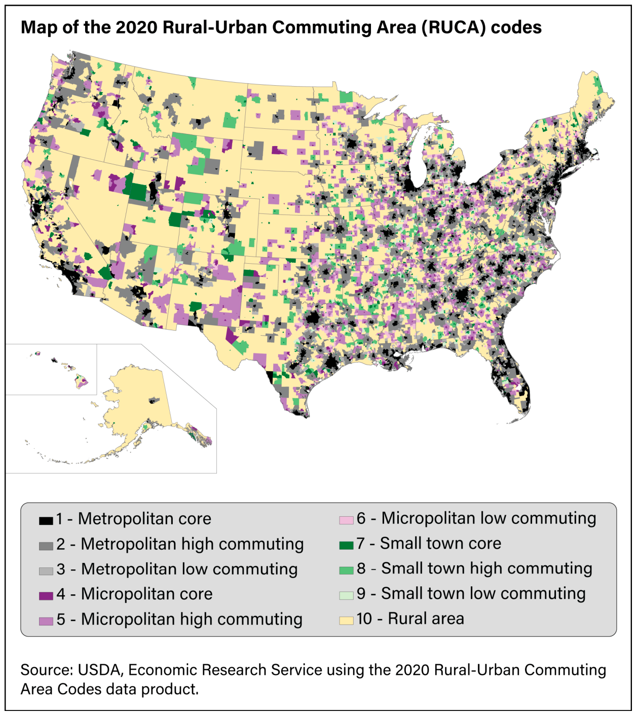
Figure 2.
Coterminous United States map of economic diversity risk clustering outcome.
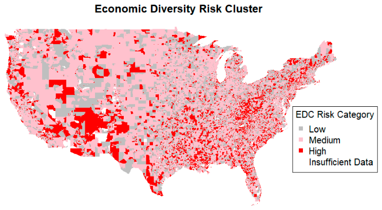
Figure 3.
Coterminous United States map of demographic diversity risk clustering outcome.
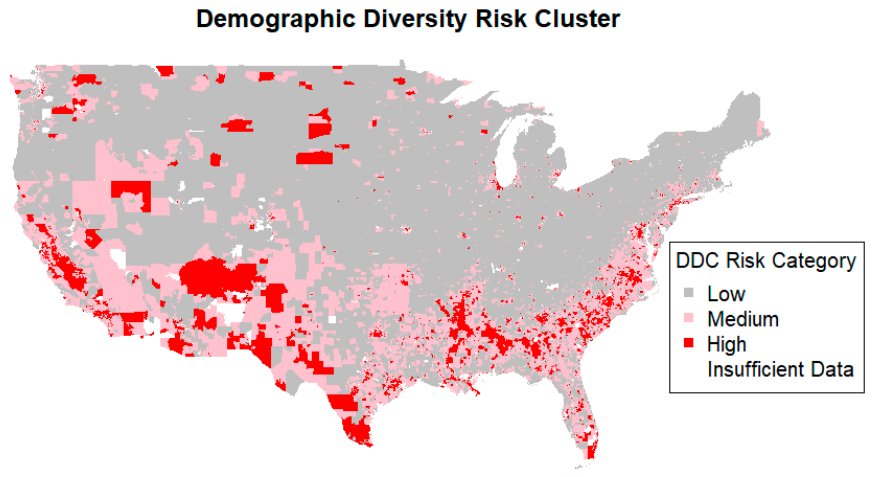
Figure 4.
Coterminous United States map of housing cost risk clustering outcome.
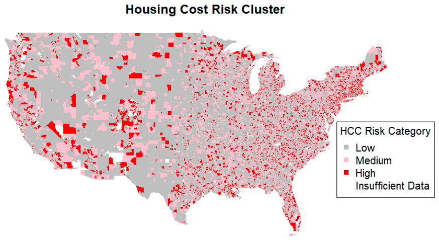
Figure 5.
Coterminous United States map of housing quality risk clustering outcome.
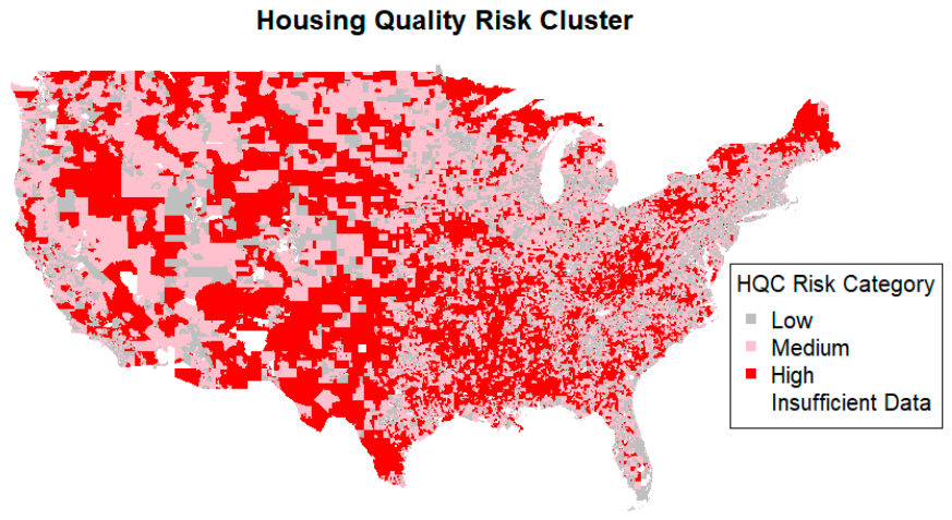
Figure 6.
Coterminous United States map of household factors risk clustering outcome.
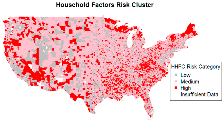
Figure 7.
Coterminous United States map of residential mobility risk clustering outcome.
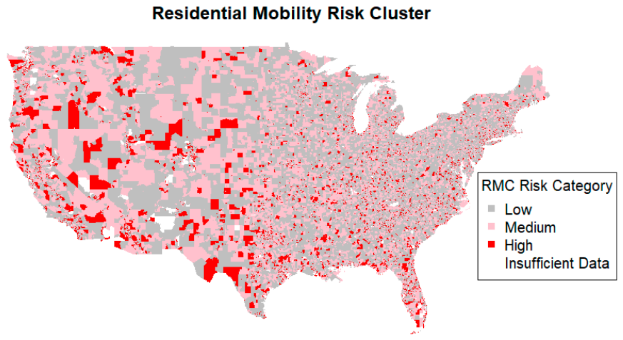
Figure 8.
Coterminous United States map of renter/owner characteristics risk clustering outcome.
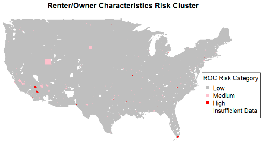
Figure 9.
Coterminous United States map showing the amount of high risk clusters in each census tract.
Figure 9.
Coterminous United States map showing the amount of high risk clusters in each census tract.
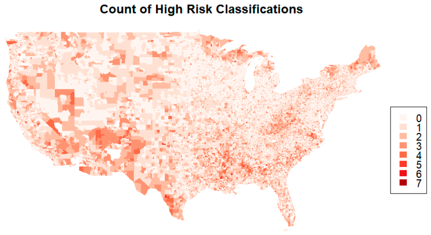
Table 1.
RUCA code designations and descriptions [18].
Table 1.
RUCA code designations and descriptions [18].
| RUCA Code | Description | Image | Example Location |
| 1 | Metropolitan core: primary flow is within an urban area of 50,000 or more people (metro UA) |  |
Portland, ME |
| 2 | Metropolitan high commuting: primary flow is 30 percent or more to a metro UA |  |
Standish, ME (to Portland, ME) |
| 3 | Metropolitan low commuting: primary flow is 10 percent to 30 percent to a metro UA | 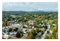 |
Livermore Falls, ME (to Lewiston/Auburn, ME) |
| 4 | Micropolitan core: primary flow is within an urban area of 10,000 to 49,999 people (micro UA) | 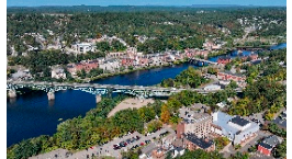 |
Augusta, ME |
| 5 | Micropolitan high commuting: primary flow is 30 percent or more to a micro UA |  |
Phippsburg, ME (to Brunswick, ME) |
| 6 | Micropolitan low commuting: primary flow is 10 percent to 30 percent to a micro UA |  |
Fairfield, ME (to Waterville, ME) |
| 7 | Small town core: primary flow is within an urban area of 9,999 or fewer people (small town UA) |  |
Presque Isle, ME |
| 8 | Small town high commuting: primary flow is 30 percent or more to a small town UA | 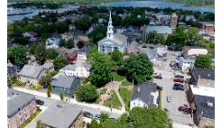 |
Warren, ME (to Rockland, ME) |
| 9 | Small town low commuting: primary flow is 10 percent to 30 percent to a small town UA |  |
Searsport, ME (to Belfast, ME) |
| 10 | Rural area: primary flow is to a tract outside an UA |  |
Farmington, ME |
Table 2.
Average silhouette scores for risk cluster outcomes from Appendix A. All dimensions other than household factors have a meaningful global silhouette score, with renter-owner characteristics having a strong silhouette score. Low risk clusters have the highest silhouette scores within their dimensions.
| Risk Factor | Low Cluster | Medium Cluster | High Cluster | Global |
| Economic Diversity (EDC) | 0.40 | 0.20 | 0.16 | 0.26 |
| Demographic Diversity (DDC) | 0.56 | 0.42 | 0.24 | 0.43 |
| Housing Cost (HCC) | 0.41 | 0.36 | 0.19 | 0.34 |
| Housing Quality (HQC) | 0.79 | 0.05 | 0.01 | 0.41 |
| Household Factors (HHFC) | 0.34 | 0.25 | -0.02 | 0.21 |
| Residential Mobility (RMC) | 0.59 | 0.21 | 0.03 | 0.33 |
| Renter/Owner Characteristics (ROC) | 0.84 | -0.11 | 0.04 | 0.72 |
Table 3.
Proportion of census tracts having a high risk designation in each of the risk categories established in Appendix A (data from Prop H columns in Appendix B).
Table 3.
Proportion of census tracts having a high risk designation in each of the risk categories established in Appendix A (data from Prop H columns in Appendix B).
| RUCA | EDC | DDC | HCC | HQC | HHFC | RMC | ROC |
| 1 | 32.60% | 35.22% | 27.00% | 8.44% | 25.71% | 23.50% | 0.76% |
| 2 | 16.80% | 7.91% | 16.12% | 15.59% | 11.04% | 9.61% | 0.02% |
| 3 | 14.57% | 6.72% | 12.91% | 25.39% | 16.06% | 5.85% | 0.00% |
| 4 | 44.27% | 13.80% | 24.35% | 18.74% | 39.63% | 27.22% | 0.22% |
| 5 | 23.81% | 5.56% | 12.29% | 30.85% | 18.34% | 8.70% | 0.00% |
| 6 | 17.27% | 5.81% | 10.74% | 32.51% | 24.09% | 5.37% | 0.00% |
| 7 | 43.72% | 12.83% | 23.06% | 25.46% | 49.97% | 22.44% | 0.27% |
| 8 | 23.85% | 5.92% | 11.51% | 43.26% | 26.32% | 7.24% | 0.00% |
| 9 | 16.96% | 8.04% | 11.61% | 38.69% | 32.14% | 3.87% | 0.00% |
| 10 | 23.09% | 8.21% | 13.40% | 38.78% | 32.29% | 9.40% | 0.05% |
Table 4.
Association rules between high risk tracts within the different factors, sorted by lift. A total of 19 combinations have a confidence of at least 30%. These rules are not necessarily symmetric, however some of them are.
Table 4.
Association rules between high risk tracts within the different factors, sorted by lift. A total of 19 combinations have a confidence of at least 30%. These rules are not necessarily symmetric, however some of them are.
| Lhs | Rhs | Support | Confidence | Coverage | Lift | Count |
| {ROC=H} | {HHFC=H} | 0.003451 | 0.634091 | 0.005442 | 2.477861 | 279 |
| {ROC=H} | {RMC=H} | 0.002684 | 0.493182 | 0.005442 | 2.446093 | 217 |
| {ROC=H} | {DDC=H} | 0.003265 | 0.6 | 0.005442 | 2.22997 | 264 |
| {ROC=H} | {EDC=H} | 0.003426 | 0.629545 | 0.005442 | 2.074834 | 277 |
| {HHFC=H} | {HCC=H} | 0.115651 | 0.451936 | 0.255903 | 1.907462 | 9351 |
| {HCC=H} | {HHFC=H} | 0.115651 | 0.488124 | 0.23693 | 1.907462 | 9351 |
| {ROC=H} | {HCC=H} | 0.002226 | 0.409091 | 0.005442 | 1.72663 | 180 |
| {HQC=H} | {HHFC=H} | 0.055606 | 0.402075 | 0.138297 | 1.571203 | 4496 |
| {HHFC=H} | {EDC=H} | 0.119733 | 0.467885 | 0.255903 | 1.542038 | 9681 |
| {EDC=H} | {HHFC=H} | 0.119733 | 0.394611 | 0.30342 | 1.542038 | 9681 |
| {RMC=H} | {HHFC=H} | 0.072834 | 0.361244 | 0.20162 | 1.411647 | 5889 |
| {DDC=H} | {EDC=H} | 0.113833 | 0.423075 | 0.269062 | 1.394356 | 9204 |
| {EDC=H} | {DDC=H} | 0.113833 | 0.375168 | 0.30342 | 1.394356 | 9204 |
| {RMC=H} | {HCC=H} | 0.06367 | 0.315789 | 0.20162 | 1.332837 | 5148 |
| {HQC=H} | {EDC=H} | 0.055903 | 0.404221 | 0.138297 | 1.332218 | 4520 |
| {EDC=H} | {HCC=H} | 0.09381 | 0.309175 | 0.30342 | 1.304921 | 7585 |
| {HCC=H} | {EDC=H} | 0.09381 | 0.395939 | 0.23693 | 1.304921 | 7585 |
| {HQC=H} | {DDC=H} | 0.04701 | 0.339921 | 0.138297 | 1.263357 | 3801 |
| {RMC=H} | {EDC=H} | 0.074467 | 0.369341 | 0.20162 | 1.217262 | 6021 |
Table 5.
The number of census tracts that have x number of high risk factors. While there is a larger risk of 1 high risk factor than 0, the number declines precipitously as the risk count climbs.
Table 5.
The number of census tracts that have x number of high risk factors. While there is a larger risk of 1 high risk factor than 0, the number declines precipitously as the risk count climbs.
| Number of Comorbidities | Number of Occurrences |
| 0 | 21,485 |
| 1 | 26,586 |
| 2 | 17,927 |
| 3 | 9,418 |
| 4 | 4,036 |
| 5 | 1,201 |
| 6 | 197 |
| 7 | 5 |
Table 6.
Presence of absence of a particular association rule, separated by RUCA codes for all combinations of two high risk categories. No association rule is universal; some association rules only arise when looking at individual RUCA codes; if an association rule exists in the entire dataset, it also appears in RUCA code 1.
| Antecedent | Consequent | ALL | 1 | 2 | 3 | 4 | 5 | 6 | 7 | 8 | 9 | 10 |
| {ROC=H} | {RMC=H} | 1 | 1 | 0 | 0 | 1 | 0 | 0 | 1 | 0 | 0 | 0 |
| {ROC=H} | {EDC=H} | 1 | 1 | 0 | 0 | 1 | 0 | 0 | 0 | 0 | 0 | 0 |
| {ROC=H} | {DDC=H} | 1 | 1 | 0 | 0 | 0 | 0 | 0 | 0 | 0 | 0 | 0 |
| {ROC=H} | {HQC=H} | 0 | 0 | 0 | 0 | 0 | 0 | 0 | 0 | 0 | 0 | 0 |
| {ROC=H} | {HCC=H} | 1 | 1 | 0 | 0 | 0 | 0 | 0 | 0 | 0 | 0 | 0 |
| {ROC=H} | {HHFC=H} | 1 | 1 | 0 | 0 | 0 | 0 | 0 | 0 | 0 | 0 | 0 |
| {RMC=H} | {ROC=H} | 0 | 0 | 0 | 0 | 0 | 0 | 0 | 0 | 0 | 0 | 0 |
| {RMC=H} | {EDC=H} | 1 | 1 | 0 | 0 | 1 | 1 | 0 | 1 | 1 | 0 | 0 |
| {RMC=H} | {DDC=H} | 0 | 1 | 0 | 0 | 0 | 0 | 0 | 0 | 0 | 0 | 0 |
| {RMC=H} | {HQC=H} | 0 | 0 | 0 | 0 | 0 | 1 | 1 | 0 | 1 | 0 | 1 |
| {RMC=H} | {HCC=H} | 1 | 1 | 0 | 0 | 0 | 0 | 0 | 0 | 0 | 0 | 0 |
| {RMC=H} | {HHFC=H} | 1 | 1 | 0 | 0 | 1 | 0 | 1 | 1 | 1 | 1 | 1 |
| {EDC=H} | {ROC=H} | 0 | 0 | 0 | 0 | 0 | 0 | 0 | 0 | 0 | 0 | 0 |
| {EDC=H} | {RMC=H} | 0 | 0 | 0 | 0 | 1 | 0 | 0 | 0 | 0 | 0 | 0 |
| {EDC=H} | {DDC=H} | 1 | 1 | 0 | 0 | 0 | 0 | 0 | 0 | 0 | 0 | 0 |
| {EDC=H} | {HQC=H} | 0 | 0 | 0 | 1 | 0 | 1 | 1 | 0 | 1 | 1 | 1 |
| {EDC=H} | {HCC=H} | 1 | 1 | 0 | 0 | 0 | 0 | 0 | 0 | 0 | 0 | 0 |
| {EDC=H} | {HHFC=H} | 1 | 1 | 0 | 0 | 1 | 0 | 1 | 1 | 1 | 1 | 1 |
| {DDC=H} | {ROC=H} | 0 | 0 | 0 | 0 | 0 | 0 | 0 | 0 | 0 | 0 | 0 |
| {DDC=H} | {RMC=H} | 0 | 0 | 0 | 0 | 0 | 0 | 0 | 0 | 0 | 0 | 0 |
| {DDC=H} | {EDC=H} | 1 | 1 | 1 | 0 | 1 | 1 | 1 | 1 | 1 | 0 | 1 |
| {DDC=H} | {HQC=H} | 0 | 0 | 0 | 1 | 1 | 1 | 1 | 1 | 1 | 1 | 1 |
| {DDC=H} | {HCC=H} | 0 | 0 | 0 | 0 | 0 | 0 | 0 | 0 | 0 | 0 | 0 |
| {DDC=H} | {HHFC=H} | 0 | 0 | 0 | 0 | 1 | 0 | 1 | 1 | 1 | 1 | 1 |
| {HQC=H} | {ROC=H} | 0 | 0 | 0 | 0 | 0 | 0 | 0 | 0 | 0 | 0 | 0 |
| {HQC=H} | {RMC=H} | 0 | 0 | 0 | 0 | 0 | 0 | 0 | 0 | 0 | 0 | 0 |
| {HQC=H} | {EDC=H} | 1 | 1 | 0 | 0 | 1 | 0 | 0 | 1 | 0 | 0 | 0 |
| {HQC=H} | {DDC=H} | 1 | 1 | 0 | 0 | 0 | 0 | 0 | 0 | 0 | 0 | 0 |
| {HQC=H} | {HCC=H} | 0 | 1 | 0 | 0 | 0 | 0 | 0 | 0 | 0 | 0 | 0 |
| {HQC=H} | {HHFC=H} | 1 | 1 | 0 | 0 | 1 | 0 | 1 | 1 | 0 | 1 | 1 |
| {HCC=H} | {ROC=H} | 0 | 0 | 0 | 0 | 0 | 0 | 0 | 0 | 0 | 0 | 0 |
| {HCC=H} | {RMC=H} | 0 | 0 | 0 | 0 | 1 | 0 | 0 | 0 | 0 | 0 | 0 |
| {HCC=H} | {EDC=H} | 1 | 1 | 0 | 0 | 1 | 1 | 1 | 1 | 1 | 0 | 1 |
| {HCC=H} | {DDC=H} | 0 | 0 | 0 | 0 | 0 | 0 | 0 | 0 | 0 | 0 | 0 |
| {HCC=H} | {HQC=H} | 0 | 0 | 0 | 0 | 0 | 0 | 0 | 0 | 0 | 1 | 1 |
| {HCC=H} | {HHFC=H} | 1 | 1 | 0 | 1 | 1 | 1 | 1 | 1 | 1 | 1 | 1 |
| {HHFC=H} | {ROC=H} | 0 | 0 | 0 | 0 | 0 | 0 | 0 | 0 | 0 | 0 | 0 |
| {HHFC=H} | {RMC=H} | 0 | 1 | 0 | 0 | 1 | 0 | 0 | 0 | 0 | 0 | 0 |
| {HHFC=H} | {EDC=H} | 1 | 1 | 0 | 0 | 1 | 1 | 1 | 1 | 1 | 0 | 1 |
| {HHFC=H} | {DDC=H} | 0 | 1 | 0 | 0 | 0 | 0 | 0 | 0 | 0 | 0 | 0 |
| {HHFC=H} | {HQC=H} | 0 | 0 | 1 | 1 | 0 | 1 | 1 | 0 | 1 | 1 | 1 |
| {HHFC=H} | {HCC=H} | 1 | 1 | 0 | 0 | 1 | 0 | 0 | 1 | 0 | 0 | 0 |
Table 7.
Number of comorbidities per tract at RUCA code level. RUCA Codes 1, 4, and 7 do not have their plurality in the 0 category, nor do the rural codes of 7-10. Flow categories within metropolitan and micropolitan groups (2-3; 5-6) show 0 as the plurality of that type of tract.
Table 7.
Number of comorbidities per tract at RUCA code level. RUCA Codes 1, 4, and 7 do not have their plurality in the 0 category, nor do the rural codes of 7-10. Flow categories within metropolitan and micropolitan groups (2-3; 5-6) show 0 as the plurality of that type of tract.
| 1 | 2 | 3 | 4 | 5 | 6 | 7 | 8 | 9 | 10 | Total Comorbidities | |
| 0 | 12684 | 4038 | 533 | 857 | 840 | 278 | 239 | 169 | 108 | 1739 | 21485 |
| 1 | 18031 | 2782 | 377 | 1409 | 811 | 239 | 385 | 245 | 124 | 2183 | 26586 |
| 2 | 12962 | 1145 | 163 | 1167 | 373 | 114 | 434 | 128 | 65 | 1376 | 17927 |
| 3 | 7022 | 348 | 62 | 744 | 165 | 42 | 286 | 49 | 36 | 664 | 9418 |
| 4 | 3311 | 70 | 10 | 322 | 37 | 13 | 88 | 15 | 3 | 167 | 4036 |
| 5 | 1056 | 13 | 1 | 79 | 4 | 3 | 23 | 2 | 0 | 20 | 1201 |
| 6 | 182 | 2 | 0 | 10 | 0 | 0 | 2 | 0 | 0 | 1 | 197 |
| 7 | 5 | 0 | 0 | 0 | 0 | 0 | 0 | 0 | 0 | 0 | 5 |
| Total RUCA | 55253 | 8398 | 1146 | 4588 | 2230 | 689 | 1457 | 608 | 336 | 6150 | 80855 |
| Prop w/Morbidity | 77% | 52% | 53% | 81% | 62% | 60% | 84% | 72% | 68% | 72% | 73% |
| Prop w/Comorbidity | 44% | 19% | 21% | 51% | 26% | 25% | 57% | 32% | 31% | 36% | 41% |
Table 8.
Proportion of tracts in a RUCA code with the given number of housing insecurity comorbidities. RUCA codes 2 and 3 are similar; RUCA codes 5 and 6 are similar; RUCA codes 8-10 are similar. Though they are different individually, RUCA codes 1, 4, and 7 show similar types of behavior.
Table 8.
Proportion of tracts in a RUCA code with the given number of housing insecurity comorbidities. RUCA codes 2 and 3 are similar; RUCA codes 5 and 6 are similar; RUCA codes 8-10 are similar. Though they are different individually, RUCA codes 1, 4, and 7 show similar types of behavior.
| 1 | 2 | 3 | 4 | 5 | 6 | 7 | 8 | 9 | 10 | |
| 0 | 22.96% | 48.08% | 46.51% | 18.68% | 37.67% | 40.35% | 16.40% | 27.80% | 32.14% | 28.28% |
| 1 | 32.63% | 33.13% | 32.90% | 30.71% | 36.37% | 34.69% | 26.42% | 40.30% | 36.90% | 35.50% |
| 2 | 23.46% | 13.63% | 14.22% | 25.44% | 16.73% | 16.55% | 29.79% | 21.05% | 19.35% | 22.37% |
| 3 | 12.71% | 4.14% | 5.41% | 16.22% | 7.40% | 6.10% | 19.63% | 8.06% | 10.71% | 10.80% |
| 4 | 5.99% | 0.83% | 0.87% | 7.02% | 1.66% | 1.89% | 6.04% | 2.47% | 0.89% | 2.72% |
| 5 | 1.91% | 0.15% | 0.09% | 1.72% | 0.18% | 0.44% | 1.58% | 0.33% | 0.00% | 0.33% |
| 6 | 0.33% | 0.02% | 0.00% | 0.22% | 0.00% | 0.00% | 0.14% | 0.00% | 0.00% | 0.02% |
| 7 | 0.01% | 0.00% | 0.00% | 0.00% | 0.00% | 0.00% | 0.00% | 0.00% | 0.00% | 0.00% |
Disclaimer/Publisher’s Note: The statements, opinions and data contained in all publications are solely those of the individual author(s) and contributor(s) and not of MDPI and/or the editor(s). MDPI and/or the editor(s) disclaim responsibility for any injury to people or property resulting from any ideas, methods, instructions or products referred to in the content. |
© 2026 by the authors. Licensee MDPI, Basel, Switzerland. This article is an open access article distributed under the terms and conditions of the Creative Commons Attribution (CC BY) license.
Copyright: This open access article is published under a Creative Commons CC BY 4.0 license, which permit the free download, distribution, and reuse, provided that the author and preprint are cited in any reuse.