

Submitted:
06 October 2026
Posted:
09 October 2026
You are already at the latest version
Abstract
Three-arm binary trials may require low-dose benefit over control and additional high-dose benefit. We evaluate posterior support, false-declaration control and power when both response-probability differences must reach positive minima and at least one exceeds its target. Conditioning on the shared low-dose probability under independent binomial sampling and independent beta priors gives the posterior probability of meeting this requirement. Probabilities of complete or partial attainment and expected shortfalls describe uncertainty. For tables retaining declarations when control responder counts decrease or high-dose counts increase, maximization of false-declaration probability over all configurations failing the requirement reduces to three one-dimensional paths. Certified bounds keep the saved tables' maximal false-declaration probability below 2.5%. With illustrative thresholds and uniform priors, the joint Bayesian rule's power was at most 1.3% across 24 acceptable profiles exceeding only one target per design (250 or 386 participants). Method-independent bounds constrain fixed-sample count-based rules with the same error control. At 30% control response, 200 low-dose participants, low-dose effects between a minimum and target of 7 and 10 percentage points, and an increment above 5 points, power cannot exceed approximately 14%, regardless of other group sizes. JADE MONO-2 counts illustrate retrospective reporting. The results distinguish satisfying a requirement from reliably establishing it.
Keywords:
Bayesian inference
; binary outcomes
; composite null
; dose response
; finite-sample calibration
; partial attainment
1. Introduction
Dose-ranging trials help determine whether a treatment is effective and whether a higher dose provides additional benefit [1,2]. Consider a trial with control, low-dose and high-dose groups and a binary outcome, such as response to treatment. Two differences in response probability may matter: low dose minus control, and high dose minus low dose. The first measures the benefit available at the lower dose; the second measures the additional benefit associated with the higher dose. A comparison of high dose with control gives their sum and cannot establish how much each contributes. We consider assessment of these two contributions at the planned final analysis of a fixed-sample trial, with the joint requirement specified during planning.
Development decisions may distinguish a desired effect from a smaller effect that remains acceptable [3,4]. We use this distinction to specify a target and a lower minimum for each of the two differences. Both differences must reach their minima, and at least one must exceed its target. We call this the target–minimum requirement. For example, suppose the low-dose minimum and target are 7 and 10 percentage points, and the corresponding values for the higher-dose increment are 2 and 5 points. Effects of 8 and 6 points satisfy the requirement: low-dose efficacy is below target but above its minimum, and the increment exceeds its target. Effects of 9 and 4 points fail because neither target is exceeded. These examples express a possible development requirement; they do not establish which effects should be clinically acceptable.
This requirement raises three statistical questions. First, after observing the responder counts, what is the posterior probability that the two true effects satisfy it? The posterior distribution describes uncertainty about the three group response probabilities conditional on those counts and the chosen prior. It also shows which effect may fall below its minimum or target, and by how much. Second, when should the data justify a declaration that the requirement holds? A false declaration occurs when the rule declares success although the true effects fail the requirement. Third, if the requirement does hold, how often would repeated trials with the planned group sizes make that declaration? This repeated-sampling probability is the rule’s power. It differs from the posterior probability calculated from one observed trial. An effect only slightly above its minimum may be acceptable under the requirement but difficult to distinguish from an effect below that minimum.
The requirement to meet all lower thresholds and at least one upper threshold is established in simultaneous non-inferiority and superiority testing [5,6]. Related procedures address correlated binary endpoints [7] and mixed continuous and binary endpoints [8]. In a preprint, Chen et al. [9] calibrated a combined testing procedure under a multivariate-normal model, and Kavelaars et al. [10] developed Bayesian decision rules for multiple correlated binary outcomes. These studies provide testing and decision principles. Here, the low-dose group enters the two differences with opposite signs, making their estimates dependent despite independent binomial sampling across groups. Separate dose–control tests or a test for an overall dose trend do not by themselves answer whether both adjacent differences meet their minima and at least one exceeds its target. Modelling a dose-response curve, as in multiple comparisons and modelling (MCP-Mod) [1], addresses a related but distinct question.
Kawasaki et al. [11] calculated joint probabilities that all specified differences exceed their margins in three-arm binary trials. By conditioning on the response probability in the shared group, they reduced the calculation to a one-dimensional integral. We retain that strategy and allow one effect to miss its target if it still reaches its minimum. The response-probability configurations satisfying this requirement form the acceptable region. Its complement, the null region, includes three reasons for failure: low-dose efficacy below its minimum, the higher-dose increment below its minimum, or neither target exceeded. Error control must cover all three reasons and all possible baseline response probabilities, rather than only a selected set of simulated examples.
For this target–minimum requirement, we determine how the three reasons for failure affect finite-sample error control and how proximity to a minimum limits attainable power. A decision table maps every possible triple of responder counts to declaration or non-declaration. For tables whose declarations are preserved when the control count decreases or the high-dose count increases, we reduce the null maximization to three paths and bound the false-declaration probability over each complete path. Separate power bounds apply to any fixed-sample rule using those counts with the required error control. Their purpose is to rule out sample-size choices that cannot meet a prespecified power goal under the requirement.
We compare joint Bayesian, componentwise Bayesian and frequentist rules with a common 2.5% error limit. The comparison assesses whether evaluating the acceptable region directly changes decisions under this common constraint; posterior reporting and power bounds address interpretation and planning beyond a binary declaration. In each design, we evaluated profiles at which both effects were strictly above their minima but only one exceeded its target. Under uniform priors and illustrative thresholds, the joint rule’s power never exceeded 1.3% across these profiles. The method-independent bounds also restrict power throughout ranges of partial attainment at a fixed control response probability, irrespective of the other two sample sizes (Table 1). These results identify both what the evaluated rules achieved and when changing the rule cannot overcome limited information. Published JADE MONO-2 counts [12] illustrate the posterior report using requirements specified for this analysis. Section 2, Section 3 and Section 4 define the requirement, posterior calculations and decision rules; Section 5 and Section 6 evaluate their performance and illustrate interpretation.
2. Clinical Requirements and Target–Minimum Profiles
2.1. Clinical Setting and Requirements
We consider a fixed-sample randomized trial with control (C), low-dose (L) and high-dose (H) groups. A favourable binary outcome is assessed at a common time point in a defined analysis population. Let be the fixed analysis denominator and the observed number of responders in group , and let denote the corresponding response probability. The outcome and analysis population must be defined before counting responders. The definition must state how missing assessments and events such as treatment discontinuation affect the response and denominator. Section 3 assumes that the resulting counts follow independent binomial distributions. The effects of interest are
The increment z is a between-group risk difference, not an individual patient’s response to dose escalation. The high-dose versus control difference is .
For low-dose efficacy, is the minimum acceptable effect and is the target. For the higher-dose increment, the corresponding levels are and ; the subscript I denotes the increment. All four levels are fixed thresholds on the risk-difference scale, not quantities estimated from the trial. The two comparisons may have different targets, minima and tolerated deficits; a common margin is not required. The effect pair , together with , determines the true response-probability profile . It is acceptable under the specified requirement when both effects meet their minima and at least one exceeds its target. Thus, at most one effect may fail to exceed its target, and that effect must still meet its minimum. The two partial-attainment routes are defined in Section 2.2. These are requirements on true effects, not separate declarations from the data.
One reason to use this requirement is that a development programme needs both doses to contribute: the low dose must provide a minimum benefit over control, and the high dose must provide a minimum additional benefit over the low dose. The programme may also require a target-level benefit in at least one of these comparisons. If neither target is exceeded, neither of these stronger development goals is met, even when the total high-dose versus control effect equals that of an acceptable profile. Excluding profiles that meet both minima but exceed neither target is part of this hypothetical development requirement; it does not mean that those profiles are clinically inferior to acceptable profiles. An application that regards both minima alone as sufficient should use a different region.
Before examining trial outcomes, prospective users should document the clinical rationale and external evidence supporting each minimum and the development goal defining each target. The reason for accepting either route must be prespecified separately. The tolerated losses and require clinical justification, drawing on the principle of acceptable efficacy loss used in non-inferiority margin setting [13]. The target and minimum levels are not the historical-effect and effect-preservation quantities of an active-control non-inferiority analysis; that principle does not determine the requirement to exceed at least one target. The criterion applies when both low-dose efficacy and incremental efficacy matter, rather than when only the high-dose versus control effect is relevant. The thresholds used below are illustrative and have not been clinically validated. Acceptance concerns the specified efficacy profile, not overall benefit–risk or dose selection.
2.2. Acceptable and Complete-Target Profiles
The response-probability profile satisfies . Thresholds are on the probability scale and satisfy
The last condition ensures that both targets can be exceeded simultaneously. We describe the requirement as a set of possible true response probabilities. The acceptable region contains every satisfying the target–minimum requirement, and contains those exceeding both targets:
Equality meets a minimum but does not exceed a target. These definitions concern the true profile; posterior assessment and declaration rules are introduced in Section 3 and Section 4. Under an absolutely continuous posterior, the boundaries have probability zero, but the convention remains part of the null region : the response probabilities for which the requirement fails. Section 4 controls false declarations over this entire region.
Under the stated threshold conditions,
Thus, one effect need not exceed its positive target, but the response probabilities must still satisfy . Equal responses at adjacent doses (a plateau) and reversed dose ordering are excluded. A high-dose benefit alone also fails if , even when is large. Such failure concerns this two-dose requirement, not the absence of any treatment benefit. Partial attainment, defined as , consists of two disjoint routes:
The first is termed the low-dose route because low-dose efficacy exceeds its target; the second is the increment route because the higher-dose increment exceeds its target. Profiles that meet both minima but exceed neither target are outside .
For illustration, let (Figure 1). With , the true profiles and give and : each meets both minima and exceeds one target. Their midpoint gives and exceeds neither target. Hence is non-convex, although increasing either effect cannot turn an acceptable feasible profile into an unacceptable one. The first two profiles lie on minimum boundaries and are not examples of high declaration probability under uniform error control (Section 4.4).
No separate high-dose versus control requirement is imposed. For a proposed threshold on that contrast, the requirement follows from if and only if
For the illustrative thresholds, every acceptable profile has . Supporting Information S1.4 establishes this sharp lower limit.
3. Joint Posterior Assessment
3.1. Model and Probability of an Acceptable Profile
We use the observed responder counts to assess whether the unknown true response probabilities satisfy the joint efficacy requirement. The posterior distribution describes uncertainty about after observing these counts, and hence about the effects and .
Let denote the random number of responders and its observed value for the fixed analysis denominator of Section 2. Write and . We assume independent binomial sampling and independent beta prior distributions for the three response probabilities,
where the positive prior parameters are fixed inputs; for prospective use they are prespecified before the trial. The base setting uses . The posteriors are independent across groups, with
Throughout this section, conditioning on means conditioning on . The group-specific shape is distinct from the error limit used in Section 4. Let and denote the posterior density and distribution function of , extending to zero for and one for . Although the three response probabilities are independent in the posterior, the contrasts and share and are dependent in the posterior: (S2.1).
The posterior probability that both effects meet their minima and at least one exceeds its target is
Thus, is posterior support for an acceptable true profile: the probability assigned to under the model, prior and observed data. It is neither a future-trial success probability nor a repeated-trial declaration rate.
To calculate joint exceedance of thresholds a and b, fix the shared low-dose probability at . The control and high-dose probabilities remain independent. Averaging over the posterior distribution of gives [11]
The formula holds for real contrast thresholds a and b. For the positive thresholds used here, the integrand vanishes outside ; if . An acceptable profile either exceeds the low-dose target and meets the increment minimum, or meets the low-dose minimum and exceeds the increment target. Adding these two probabilities and subtracting their overlap gives (derivations in Supporting Information S2)
Marginal probabilities such as and describe the effects separately. Their product generally differs from because it ignores the dependence induced by .
3.2. Attainment States and Shortfall Summaries
Different datasets can have similar overall posterior probability while assigning support to different attainment states. We distinguish complete attainment, the low-dose route and the increment route of Section 2, with posterior probabilities
respectively. All three states meet both minima; they exceed both targets, only the low-dose target, or only the increment target. Together with the probability of an unacceptable profile, , they form the primary four-state report. The sum is the probability of partial attainment. A high can be spread across the three acceptable states. These probabilities describe posterior uncertainty, not separate error-controlled declarations.
The four-state report summarizes overall attainment. For a more detailed account of which requirements may fail, we further classify each effect into three states: state 0, below its minimum; state 1, at or above its minimum but not above its target; and state 2, above its target. Thus the low-dose states are , and , with analogous states for z. Conditional on , the low-dose and increment state probabilities, ordered as states 0, 1 and 2, are
Pairing the three states of each effect gives nine possible combinations. The posterior probability that the low-dose effect is in state i and the increment is in state j is
These nine probabilities sum to one, with , and . The outside probability, defined above as , is computed by summing the remaining six cells. Conditional independence given justifies the product; after averaging over , cell probabilities are not generally products of the separate state probabilities. Each profile belongs to one cell, so multiple failures are counted only once.
To describe how far each effect may fall below its target, the posterior expected shortfall averages that deficit over uncertainty about the true effect:
Here sets the deficit to zero whenever the target is reached or exceeded. Both expectations are multiplied by 100 for reporting in percentage points. Averaging includes profiles with zero deficit, unlike the conditional mean among profiles missing the target. Expected shortfall also differs from the positive part of the target minus the posterior mean effect. Conditioning on gives one-dimensional integrals involving beta partial moments: first moments integrated over specified subintervals of (Supporting Information S2).
For each effect, the mean deficit conditional on missing its target equals its unconditional expected shortfall divided by its posterior probability of missing that target, provided that probability is positive. These descriptive summaries are available regardless of the score used for the error-controlled joint declaration in Section 4.
3.3. Computation
We evaluate the beta posterior integrals without approximating the effect differences by normal distributions. The three acceptable-state probabilities are computed directly from the non-negative integrands , and , and added to obtain . This avoids recovering a small state probability by subtracting two much larger probabilities. Numerical integration must also account for small tail probabilities and changes in the integrand at the threshold boundaries. Supporting Information S2 gives the integration details, partial-moment formulas and computational checks.
Numerical integration error estimates and comparisons across precision settings check numerical stability; they do not provide proved intervals containing the exact posterior probabilities. Section 4 establishes error control separately by bounding the saved rule’s maximal false-declaration probability over all unacceptable true profiles.
ChatGPT (OpenAI) assisted with literature searches, code-related work, and mathematical and statistical checks during manuscript preparation. Its use and the authors’ review of the outputs are disclosed in the Acknowledgments.
4. Frequentist Calibration and Limits on Declaration Probability
4.1. Declaration Rule and False-Declaration Probability
A joint declaration is the trial’s conclusion, based on the responder counts, that both effects meet their minima and at least one exceeds its target. We calibrate the decision rule to limit how often it makes this declaration when the true profile fails the requirement.
Fix the analysis denominators, independent beta priors and four thresholds of Section 2 and 3. The joint posterior rule declares when the posterior probability exceeds a fixed cutoff c. Using the exact posterior probability gives the ideal rule
Here is one when its condition holds and zero otherwise. Any fixed deterministic rule can be represented as a binary decision table : for every possible count triple , the table stores one for declaration or zero for no declaration. For a fixed true profile , its declaration probability over repeated trials is
The sum weights every decision by the probability of its count triple and is continuous on . Unlike , which describes uncertainty after observing the data, describes variation in trial decisions at fixed true response probabilities.
The null comprises all unacceptable true profiles: the low-dose effect is below its minimum, the increment is below its minimum, or neither effect exceeds its target. A declaration at any such profile is false. The maximal false-declaration probability is , where
For a true profile in , is the power to declare the joint requirement; its supremum over is the maximal type I error. The three null components overlap because a profile can fail more than one condition. The central-cell probability of Section 3 is the posterior probability of , where both minima are met but neither target is exceeded; also includes profiles below one or both minima.
Two monotonicity conditions simplify maximization. Holding the other counts fixed, is non-increasing in the control count and non-decreasing in the high-dose count. For a fixed denominator and prior, a larger responder count shifts that group’s beta posterior towards higher response probabilities. Decreasing or increasing preserves membership in ; posterior independence therefore gives these two monotonicity conditions for and .
For any decision table satisfying these two monotonicity conditions, binomial stochastic ordering gives corresponding directions in repeated-sampling probability: is non-increasing in and non-decreasing in , with the other probabilities fixed. No monotonicity in the low-dose count or response probability is assumed: increasing improves x but reduces z. Supporting Information S3 supplies the ordering arguments.
4.2. Reduction to Three Paths
These two monotonicity conditions reduce maximization over the three-dimensional null to three one-dimensional paths, one for each null component. Each path fixes and chooses the control and high-dose probabilities giving the largest declaration probability within that component or its boundary. In the order , define, for ,
Theorem 1.
Under the threshold conditions of Section 2, independent binomial sampling and fixed positive denominators, let be a fixed binary table that is non-increasing in and non-decreasing in for every fixed . Then
At fixed , decreasing and increasing gives the limiting paths , and for , and , respectively. Continuity includes boundary values approached from the strict null components and ; belongs to . The path suprema are attained, although a maximizing point can lie on the boundary rather than inside the corresponding strict null component. Supporting Information S3 gives the proof.
The maximum and minimum operations keep response probabilities between zero and one. On , both target equalities hold only for ; the outer pieces remain part of the null. Maximization must cover entire paths, including these pieces. The reduction also applies to comparison tables satisfying Theorem 1’s two monotonicity conditions.
4.3. Finite-Sample Calibration
Calibration is applied to the decision table that will actually be used. We bound its false-declaration probability over each of the three paths and certify the table only when all three bounds are at most . This limits the probability of a false declaration to 2.5% at every unacceptable true profile. A posterior cutoff of 0.975 does not itself establish this repeated-sampling property.
The computed posterior score can differ from the exact . We denote the implemented joint score by and its decision table by . A tilde denotes an implementation score; and are the corresponding comparison scores defined in Section 5.1. The score construction satisfies the two monotonicity conditions required by Theorem 1, using the same adjusted score array for every candidate cutoff. Supporting Information S4.2 gives the rounding and monotone-adjustment details. This construction does not establish a bound on the exact posterior score.
Let be a proved upper bound on the table’s largest declaration probability anywhere along path k. Verifying gives
and certifies the saved table. Because this calculation bounds the sampling probability of the saved decisions, it does not require proved intervals containing the exact posterior scores.
For a fixed table, each path probability is a polynomial between the points where clipping at zero or one changes the path formula. A Bernstein representation expresses the polynomial as a weighted average of coefficients, so the largest coefficient bounds the polynomial throughout that interval. Subdividing the interval can tighten these bounds. In the main evaluation, integer coefficient construction and rational Bernstein subdivision supplied bounds over every path piece. Numerical searches guided candidate selection; certified bounds determined acceptance. Supporting Information S4 gives the arithmetic details and the separate score-precision checks.
Algorithm 1: implementation-table calibration.
- 1.
- Fix the score construction, cutoff convention, candidate family and verification settings (S4). Include the empty table that never declares.
- 2.
- Construct nested candidate tables, so that more-permissive candidates retain all previous declarations. Bound each candidate’s complete null paths using Theorem 1. A candidate is safe when its upper bound is at most , invalid when a lower bound exceeds , and otherwise unresolved.
- 3.
- Select the most permissive verified safe candidate considered. Unresolved more-permissive candidates prevent a claim of being most permissive within the family, but do not invalidate the selected table’s guarantee.
- 4.
- Save the table and its path certificates before evaluating power. Store the table as the minimum high-dose responder count required at each control and low-dose count pair, including a value for pairs at which declaration is impossible.
In the Section 5 evaluation, each selected table’s immediately more-permissive neighbour exceeded the error limit. The selected table was therefore the most permissive valid table within its fixed numerical-score family, without implying optimality among ideal-score rules or arbitrary tests.
To apply the certified rule, use the archived count boundaries; changing a boundary requires renewed certification. The guarantee can be extended to the ideal rule if its declaration set is separately proved to agree with, or be contained within, that of a certified table.
This distinction affects error control in practice. For the 386-participant design D386 described in Section 5, applying the archived full-precision cutoff to the ideal posterior rule gives a false-declaration probability greater than 2.5169% at a specified null point (S4.8). Even a tiny score difference can change the binary decision at a count triple with positive sampling probability; score accuracy alone therefore does not establish the same error bound. The guarantee applies to the separately certified saved table.
4.4. Boundary Behaviour and Limits on Declaration Probability
An acceptable profile may be difficult to distinguish from an unacceptable one. The following bounds can rule out a planned sample size when the desired power exceeds the bound. They limit declaration probability for any rule satisfying the full-null error constraint. A fixed decision function may here take values in , representing the probability of declaring after observing a given count triple. This allows mathematical randomization, although the proposed implementation is deterministic. The notation denotes the null together with all limits of sequences of null profiles.
Proposition 1.
If , then for every .
By continuity, an acceptable profile approached by null profiles cannot have declaration probability above the error limit. This includes the Section 2 examples with an effect exactly at its minimum. For interior acceptable profiles, we report distances from relevant boundaries; null and boundary profiles serve as error-control checks.
A second bound compares a chosen alternative profile with a single point in the null or its closure.
Proposition 2.
For any rule with the same uniform error constraint, any and any alternative ,
where is the power of the most powerful level- test of the simple null against . Here, a simple null or alternative specifies one complete response-probability profile, and level requires declaration probability at most at that null profile.
Uniform control and continuity make the rule level at ; the Neyman–Pearson (NP) lemma gives the bound [14]. Taking the minimum of bounds from several such null or null-closure points remains valid. If the two profiles differ in only one group, the other groups have identical sampling distributions under both profiles, so only that group’s count enters the likelihood ratio (Supporting Information S5).
For partial attainment through the increment route, this comparison gives a bound depending only on the low-dose sample size once the control response probability is fixed. The set of profiles at that fixed control probability is called a fixed-baseline slice.
Corollary 1 (Fixed-baseline partial-attainment bound).
Under the independent-binomial model with fixed positive denominators and the threshold conditions of Section 2, let be fixed and satisfy , with . Let be the power of the randomized most powerful level- binomial test of u against , with . Fix with . Every feasible increment-route profile satisfying and obeys
To obtain the first inequality, compare with the null-closure point , which places the low-dose effect exactly at its minimum. Only the low-dose distribution changes between these profiles. The second inequality follows because the power of the upper-tail binomial test increases as the alternative low-dose response probability increases. Unlike Theorem 1, the corollary requires no monotonicity of the evaluated decision rule. Fixing r restricts the profiles being evaluated; the rule must still control error over the full null, including other control response probabilities.
With the illustrative thresholds and , the bound is . Table 1 shows its values throughout the feasible increment-route slice at this fixed baseline, irrespective of the control and high-dose sample sizes. To have 80% power at even one profile in this fixed-baseline increment-route slice requires . This is a necessary condition, not a sufficient sample-size requirement. Supporting Information S5 gives the exact values, the point-specific 11.02% bound, and the analogous low-dose-route result at fixed .
The bound also describes what happens when the allowed gap between the low-dose minimum and target becomes small. For fixed and , the upper bound converges to as through feasible specifications. Thus, for any family of rules each controlling its corresponding full null, the limit superior of the maximal declaration probabilities over these fixed-baseline increment-route slices is at most , even if the other groups’ sample sizes increase (S5.9). Actual declaration probabilities need not converge to . These are upper limits, not statements that a rule attains them; their numerical values depend on the baseline and do not apply unchanged to complete-target profiles.
5. Numerical Evaluation
5.1. Objectives, Scenarios and Methods
The evaluation addressed three questions: whether the implemented rules control false declarations over the full null, how often they declare at specified true profiles, and what posterior reports reveal about unmet targets. Declaration probabilities describe repeated-trial decisions, whereas posterior summaries describe uncertainty after each dataset. Method-independent power bounds provide benchmarks that no valid rule can exceed, but need not be attainable.
We used the illustrative thresholds . Thus the low-dose versus control effect had a minimum of 7 and a target of 10 percentage points, and the high-dose versus low-dose increment had a minimum of 2 and a target of 5 percentage points. Designs D250 and D386, named for their total sample sizes, used fixed denominators and , respectively, in control, low-dose and high-dose order.
Eighteen effect pairs at each control response probability , and gave 54 evaluation points per design (Table 2; Supporting Information S6.1). Varying the baseline while holding the effect differences fixed preserves the attainment state and assesses sensitivity to baseline-dependent binomial sampling variability. Complete-target profiles exceed both targets; near and farther denote smaller and larger excesses. The low-dose route exceeds the low-dose target while the increment lies between its minimum and target; the increment route reverses these roles. Within each partial route, locates the effect between minimum and target, and is the other effect’s excess above target, in percentage points. Four combinations per route and baseline give 24 interior partial-attainment points per design. The remaining profiles examine unmet minima or targets, equality at a minimum or both targets, a plateau with no increment, and a reversed increment. Minimum-boundary profiles also belong to but are evaluated separately as boundary diagnostics. These points were used to evaluate fixed rules; calibration covered the entire null region.

Table 2.
Fixed designs and true-effect profiles used in the numerical evaluation.
| Design | Total | |||
| D250 | 50 | 100 | 100 | 250 |
| D386 | 77 | 155 | 154 | 386 |
| True-effect family | x (pp) | z (pp) | Profiles per baseline |
In | In |
| Complete target, near | 12 | 7 | 1 | Yes | Yes |
| Complete target, farther | 20 | 15 | 1 | Yes | Yes |
| Low-dose route | 4 | Yes | No | ||
| Increment route | 4 | Yes | No | ||
| Neither target exceeded | 8.5 | 3.5 | 1 | No | No |
| Low-dose minimum not met | 5 | 15 | 1 | No | No |
| Increment minimum not met | 20 | 1 | 1 | No | No |
| Plateau | 20 | 0 | 1 | No | No |
| Reversed increment | 20 | -2 | 1 | No | No |
| Low-dose minimum boundary | 7 | 15 | 1 | Yes | No |
| Increment minimum boundary | 20 | 2 | 1 | Yes | No |
| Both-target corner | 10 | 5 | 1 | No | No |
All thresholds are illustrative: percentage points (pp). In each family, , and , converting effects from pp to probabilities. For partial routes, and pp yield four combinations. Thus, 18 effect profiles at three baselines give 54 points per design. Minimum equalities belong to but are used for boundary diagnostics, not as high-power design points. The two designs differ in both sample size and allocation; their comparison is not a pure sample-size contrast. Full coordinates and boundary distances are supplied in Data S1; Supporting Information S6.1 identifies the corresponding file. Three implemented rules addressed the same acceptable region , with a maximal false-declaration limit over all true profiles outside it. Both Bayesian rules used independent priors. The joint Bayesian rule used the posterior probability of satisfying the joint target–minimum requirement. The componentwise Bayesian rule combined the separate posterior probabilities of exceeding each threshold, using
where and . Its score requires support for both minima and at least one target, but does not calculate their joint posterior probability. The frequentist union–intersection/intersection–union (UI–IU) comparator combined one-sided component tests using
The outer maximum requires both minimum tests and the target component to pass; the inner minimum permits either target test to supply the target evidence. Here and are component p-values for and . Each is the largest, over its component null, binomial probability of a risk difference at least as large as the observed one, including ties. For these ideal p-values, the factor two provides the Bonferroni adjustment for the two target tests. The numerical decision table was calibrated over the full null separately, without assuming that approximate p-values retain this guarantee.
The unconditional calculation sums over possible counts in both groups without conditioning on their total. Let be the control and low-dose response probabilities for the first contrast, or the low-dose and high-dose probabilities for the second. Each supremum reduces to the boundary , ; numerical maximization retained the whole interval. The comparator used no prior. Neither V nor W is a posterior probability of .
Let and denote the Bayesian scores’ calibrated upper-tail cutoffs, and the frequentist score’s calibrated cutoff used with ≤. The numerical implementations declared when or , respectively; the frequentist implementation declared when . A tilde identifies the fixed numerical score defining the saved table. Integer cross-products preserved risk-difference ties. The specification and code were fixed before calibration, but after preliminary feasibility calculations and examination of the retrospective dataset; this was not prospective clinical prespecification. At the specified rational profiles, declaration probabilities were computed by exact rational evaluation of the binomial finite sums, so no Monte Carlo standard errors apply.
We also evaluated a complete-target reference rule based on , the posterior probability that both targets are exceeded. Its implementation declared when the numerical score exceeded a cutoff calibrated separately over . Because that null includes partial-attainment profiles accepted by , this reference addresses a stricter requirement, rather than efficiency for the same declaration (S6.6).
An exploratory sensitivity analysis of the target-component weighting examined
which omits the factor two from that component. Each implementation was recalibrated over the full composite null. Exploratory analyses also examined repeated-trial decision disagreement and tighter power bounds from alternative null comparison points. The rates and disagreement probabilities used deterministic floating-point binomial sums. These analyses were specified after the main results and did not alter the main comparison (S5.8 and S6.8–S6.9; Data S2).
Reporting and rounding conventions are given at the start of Supporting Information S6.
5.2. Calibration and Computational Performance
All six primary decision tables satisfied the 2.5% maximal false-declaration limit over the full null region (Table 3). Six additional tables were certified separately: two for prior sensitivity, two for the complete-target reference and two for target-component weighting sensitivity. All twelve tables declared for at least one possible dataset. Their maximal false-declaration probabilities were below 0.025 over the corresponding null regions: for ten tables and for the two complete-target reference tables.
For the implemented joint Bayesian, componentwise Bayesian and frequentist UI–IU rules, the certified upper bounds were 2.4694%, 2.4694% and 2.1029% in D250. The corresponding D386 bounds were 2.4951%, 2.4951% and 2.4949% (Table 3). These are outward-rounded bounds on repeated-sampling false-declaration probabilities, not confidence limits. Both Bayesian rules attained their maxima on , where only configurations contribute; the small probability of their disagreements there explains the matching displays despite distinct tables (S6.2). In D250, W used less of the common error allowance than the Bayesian rules. No table attained its maximum on the third null path; this setting-specific finding does not justify omitting that path generally.
For every selected table, the immediately more-permissive candidate violated the error limit. The selected table was therefore the most permissive valid table in that fixed numerical-score family. The guarantee concerns the saved decisions, without asserting their agreement with ideal-score decisions at every count configuration. Score construction and verification details are given in S4 and S6.2; the two calibrations are in S6.8.
Per-rule calibration took 5.98–9.82 seconds in D250 and 57.02–74.86 seconds in D386 for the six main comparisons (Table 3). These timings exclude shared score construction, independent certificate verification and performance evaluation. S6.2 reports construction times alongside the calibration and verification records. These measurements do not describe cost at unexamined sample sizes.
5.3. Declaration Probabilities and Feasibility Bounds
Power to declare was low at the 24 interior partial-attainment profiles per design (Figure 2A–B; Figure S6.1 shows the rate-only enlargement). In D250, the largest declaration probabilities were 0.364% for the joint Bayesian rule, 0.388% for the componentwise Bayesian rule and 0.140% for the frequentist UI–IU rule. In D386, the respective maxima were 1.274%, 1.120% and 0.456%. Each maximum was taken separately across the 24 evaluated points for that rule and design; none is a maximum over the continuous partial-attainment region.
Across the 48 partial-attainment design/profile combinations, the point-specific most-powerful-test upper bounds had a maximum of approximately 11.32%. Each compares a true profile with a chosen null or null-limit profile and bounds the power of every rule controlling false declarations over the full null (Section 4.4). Figure 2 also gives the distance above the minimum for the effect that does not exceed its target and the excess above target for the other effect. The implemented rates were lower than the bounds. This gap does not quantify avoidable inefficiency: a rule attaining a bound for one null comparison need not control error over the entire composite null.
Power was also limited at complete-target profiles with : joint-rule rates ranged from 5.93% to 10.06% across the three baselines in D250 and from 18.97% to 31.94% in D386 (Figure S6.2). Because the designs also differ in allocation, their differences are not solely sample-size effects. The joint and componentwise Bayesian rules had no uniform ordering of declaration rates. Among the partial-attainment points, the largest positive difference in favour of the joint rule was approximately 0.164 percentage points in D386 and below 0.001 percentage points in D250. Full profile-specific rates and differences are supplied in Data S1 and described in S6.3–S6.4.
Exploratory analyses tightened one power bound and changed the comparator’s target component, without altering the finding of low power. For D386 at , a two-group null comparison reduced the bound from 11.32% to 6.70%; it was not optimized over the null, and Figure 2 retains the original one-group bounds (S5.8). Recalibrated tables increased the largest partial-attainment rates to 0.296% in D250 and 0.891% in D386. Their maximal-error upper bounds were still 2.1029% and 2.4949%, respectively, at the displayed precision, so D250 did not compare rules at the same maximal false-declaration probability. Each table retained every declaration made by W; this inclusion concerns these specific rules, not UI–IU procedures generally (S6.8). Repeated-trial disagreement probabilities for the Bayesian rules, counting disagreements in both directions, are reported in S6.9.
5.4. Reporting Behaviour and Sensitivity
To study how posterior reports vary from trial to trial, we generated 10,000 trials at each of 12 fixed true profiles per design. The 240,000 generated trial datasets were reused under independent and priors, giving 480,000 posterior evaluations. A posterior report was calculated for each dataset and then summarized across generated trials. Means, Monte Carlo standard errors and the 10th, 50th and 90th percentiles are supplied in Data S1; S6.5 identifies the corresponding files and presents an illustrative comparison.
For illustration, two D386 profiles with the same and had and . They follow the low-dose and increment routes, respectively. Under priors, the sampling mean of was 57.61% for the low-dose route and 57.68% for the increment route. For the low-dose route, the mean posterior expected shortfalls were 0.34 percentage points for low-dose efficacy and 3.33 for the increment. For the increment route, the corresponding means were 3.29 and 0.25 percentage points. Similar overall posterior support therefore accompanied different locations of shortfall: mainly the increment for the first profile and mainly the low-dose effect for the second. These are averages of posterior summaries across repeated trials, not individual-trial reports or declaration rates. Each posterior expected shortfall includes zero when a target is met or exceeded.
After recalibration under independent priors in D386, the largest rates across the 24 partial-attainment points were 1.749% and 1.552% for and V. Declaration probabilities remained low at these points (S6.7). D250 under this prior was assessed descriptively only, without additional calibrated tables. Both priors have mean 0.5 and differ in concentration and shape. This comparison does not assess informative priors, different group-specific means or historical borrowing.
6. Retrospective Illustration: JADE MONO-2
6.1. Trial and Profile Specification
This example uses publicly reported counts from a trial whose placebo and two active-dose groups match the proposed setting. It illustrates how the final report quantifies uncertainty about target attainment beyond the observed effect differences. JADE MONO-2 was a randomized, double-blind trial of placebo and once-daily abrocitinib 100 mg and 200 mg in patients aged 12 years or older with moderate-to-severe atopic dermatitis [12]. We used the week-12 EASI-75 response, defined as at least 75% improvement from baseline in the Eczema Area and Severity Index, one of the trial’s coprimary endpoints. Placebo, 100 mg and 200 mg form the control, low-dose and high-dose groups in this illustration. The published numbers of responders and endpoint-specific analysis denominators were 8/77, 69/155 and 94/154, respectively (Table 4); the randomized denominators were 78, 158 and 155. These same published counts were used in the ordering-probability illustration of Kawasaki et al. [11]; here they illustrate the target–minimum requirement.
The article’s supplementary methods classified missing responses after permanent study discontinuation as non-response and described stratified comparisons of each dose with placebo [12] (Supplement 2). We retained the published denominators as fixed binomial inputs; individual missing-data assignments could not be reconstructed from these summaries. The unadjusted observed differences were 34.13 percentage points for low dose versus control and 16.52 for high versus low dose. The high-dose versus low-dose difference is a parallel-group contrast, not the effect of escalating treatment in individual non-responders.
We retained the illustrative thresholds used in Section 5 and independent priors. The joint requirement is therefore a low-dose effect of at least 7 percentage points and an increment of at least 2 percentage points, together with a low-dose effect above 10 percentage points or an increment above 5 percentage points. The thresholds and the choice to accept either target were introduced for this methodological illustration and were not prespecified in JADE MONO-2.
6.2. Joint Assessment and Calibrated Declaration
Under the stated prior, the posterior mean differences were 33.19 percentage points for low dose versus control and 16.31 for high versus low dose (S7.2), distinct from the observed differences reported above. The posterior probability of satisfying was 99.46%. It comprised 97.83% for complete target attainment, where both effects exceed their targets; 1.63% for the low-dose route, where only the low-dose target is exceeded and the increment meets its minimum; and 0.003% for the increment route, where only the increment target is exceeded and the low-dose effect meets its minimum. These are posterior probabilities for this dataset, not probabilities that a future trial would make a declaration. The probability of being outside was 0.54% (Table 4).
The nine-cell report in Figure 3A separates each effect into below-minimum, minimum-to-target and above-target states. Its largest outside cell, with probability 0.536%, combined a low-dose effect exceeding its target with an increment below its minimum. This cell accounted for nearly all of the outside probability, locating the remaining uncertainty principally in the between-dose increment.
The posterior expected target shortfalls were and 0.045 percentage points for the low-dose effect and increment, respectively (Figure 3B). Each averages the deficit over the entire posterior, assigning zero whenever the target is reached or exceeded. For the increment, the posterior probability of falling below target was 2.17%, and the mean deficit conditional on this event was 2.10 percentage points. Their product, using unrounded values, gives the unconditional expected shortfall of approximately 0.045 percentage points. It therefore reflects both the probability and magnitude of target failure. S7.6 reports these summaries for both effects under both priors; full-precision values remain in Data S1 and Data S2.
For this retrospective illustration, we applied the D386 joint-rule table from Section 5, which matched the published denominators and the thresholds and priors specified for this analysis. Its implemented score was 0.9946, above the cutoff 0.9761; these are rounded display values. The saved count boundary gives a direct check: at the observed , declaration required , and the published high-dose count was 94. Both comparison rules also declared . The separately calibrated complete-target reference rule declared , the stricter requirement to exceed both targets, with a minimum high-dose count of 94 at these fixed control and low-dose counts. The three primary rules for agree on a declaration in this example; the joint and attainment-state probabilities additionally show how posterior support is distributed across the acceptable states.
With independent priors, was 99.48% and was 97.90%; both recalibrated Bayesian rules retained the joint declaration (S7). Posterior mass was concentrated on complete attainment. The example therefore shows how the method reports a strongly supported complete-target profile; it does not establish high power at true partial-attainment profiles. Error control concerns the saved tables under the stated fixed-denominator binomial model. It does not cover the original trial’s missing-data process, stratified analyses, multiplicity adjustments or retrospective specification of the requirements, and the illustration does not re-establish the trial’s confirmatory conclusions.
7. Discussion
This study examined how a trial can assess and declare a joint efficacy requirement: low-dose efficacy and the higher-dose increment must both reach minimum levels, and at least one must exceed its target. Posterior probabilities describe how strongly the observed data support these conditions and which condition remains uncertain. Expected shortfalls describe the amount by which each effect may fall below its target. A separate calculation controls the probability that the decision rule declares success when the requirement is false. We implemented both steps and derived upper bounds on how often any rule with that error control can declare success when the requirement is true. Together, the results distinguish an acceptable true effect profile from a profile that a trial can reliably establish.
The requirement to meet all lower thresholds and at least one upper threshold is established in simultaneous non-inferiority and superiority testing [5,6], including methods for binary and mixed endpoints [7,8]. Calibration over the combined null has been studied for multivariate-normal endpoints [9], and Bayesian decisions for correlated binary outcomes have also been developed [10]. Kawasaki et al. [11] calculated joint probabilities that all specified differences exceed their margins in three-arm binary trials. We retain their strategy of conditioning on the shared group and allow one effect to miss its target provided it meets its minimum and the other effect exceeds its target. The principal analytical results are a three-path reduction of full-null maximization for the stated class of decision tables and finite-sample power bounds that apply independently of the chosen rule, including bounds uniform over fixed-baseline partial-attainment slices. The posterior reports and numerical comparisons show how these results inform interpretation and planning. Conditioning and polynomial bounds are computational tools, rather than new general principles. The additional failure condition, that neither target is exceeded, gives a third path on which false-declaration probabilities must be checked. That path was included in every calibration for , although it did not determine the maximum in the evaluated settings.
The numerical evaluation found low power at the specified partial-attainment profiles, despite their satisfying the requirement. Power was also limited at the evaluated complete-target profiles. D386 matches the published JADE MONO-2 endpoint denominators; neither design was selected to achieve a prespecified power for this requirement. The results therefore identify limitations of these designs under one threshold specification, rather than establishing that useful performance is impossible at larger sample sizes or at other effect profiles.
The upper bounds distinguish limitations of a particular rule from restrictions applying to every rule with the required error control. Related simultaneous non-inferiority and superiority procedures have shown low power for effects within a non-inferiority margin, with the loss varying by correlation [8]. Here, the point-specific bounds apply independently of the chosen rule, and Corollary 1 extends the restriction throughout a range of partial attainment at a fixed control response probability. At the baseline and thresholds in Table 1, increasing the control and high-dose sample sizes alone cannot remove the ceiling imposed by the low-dose sample size. To make 80% power possible at even one profile in that range requires at least 2,061 low-dose participants (S5.5). This is a necessary condition, not a sufficient sample-size recommendation. For fixed , and , narrowing the permitted low-dose shortfall towards zero drives this upper bound towards ; it does not imply that every rule’s power converges to that value (Section 4.4; S5.9).
A high upper bound does not establish feasibility: the intended rule still needs calibration and power assessment. The bounds need not be attainable under the full null, so their distance above a rule’s achieved power does not quantify avoidable inefficiency. No corresponding method-independent impossibility result was established for the evaluated complete-target profiles.
The comparisons showed no uniform superiority of the joint posterior rule. At partial-attainment points, differences from the componentwise Bayesian rule were small and depended on the setting; the largest positive difference was approximately 0.164 percentage points (Section 5.3). The frequentist comparator had a smaller maximum false-declaration probability in D250, which matters when interpreting its lower power. The sensitivity analysis also showed that changing the score can improve power after recalibration, although its maximum false-declaration probability remained below that of the joint rule in D250. A common error ceiling therefore did not give identical maximal false-declaration probabilities. These comparisons concern the specified rules and do not establish the best Bayesian or frequentist test. The posterior calculation provides an uncertainty report alongside a declaration: the probability that the entire requirement holds, which effect is mainly responsible for uncertainty, and the probability and magnitude of target shortfall. These reports can accompany a frequentist or Bayesian declaration rule; their interpretability does not establish a power advantage for the joint posterior rule.
The JADE MONO-2 analysis illustrates this distinction in one observed dataset. Most posterior probability was assigned to complete target attainment, with the remaining uncertainty principally about the high-dose versus low-dose difference. The small expected shortfall for that difference combined a low probability of falling below target with a larger mean deficit conditional on doing so. Reporting both quantities explains why a small overall mean deficit does not exclude a meaningful deficit in the less likely event of target failure. The matched decision tables also declared the requirement met. This observation concerns one dataset; it is not evidence of high power when the true effects achieve only one target.
Several restrictions define the scope of the findings. The performance evaluation used one threshold specification, two allocations, three baseline probabilities and two symmetric priors; it does not establish robustness to informative or group-specific priors or historical borrowing. If the prior is changed for decision making, the resulting table must be certified separately. The thresholds and the requirement to exceed at least one target need clinical justification before prospective use. The model assumes fixed denominators and independent binomial counts for one favourable outcome at one time point; the calibration does not cover departures from these sampling assumptions. The three-group setting isolates low-dose benefit and the increment through a shared low-dose group. Additional doses require a new joint requirement; the present integral formulas and three-path calibration have not been established for that setting. Positive minima exclude a dose-response plateau or reversal; overall benefit–risk and patient-specific responses to dose escalation were not evaluated.
The finite-sample false-declaration guarantee concerns the saved decision tables over their entire null regions under the assumed model. Recomputing exact posterior probabilities at the same cutoff defines a potentially different rule, so its error control must be verified separately (S4.8). For uniform priors and rational thresholds, exact integration could help prove that an ideal rule’s declarations are included in those of a certified table (S4.2.2); this extension was not established here.
8. Conclusions
A true effect profile can satisfy the specified efficacy requirement while the available sample sizes give little chance of declaring it with controlled error. Prospective use should begin with a clinical justification of the minima, targets and requirement that at least one target be exceeded. The upper bounds can then rule out some sample-size specifications before a decision rule is selected. If the desired power is not ruled out, the intended rule still needs calibration and evaluation of its achieved power. After a trial, report the responder counts, thresholds and prior; both component-effect estimates; and the joint and attainment-state probabilities. Pair each expected shortfall with the probability of missing its target and, when useful, the mean deficit conditional on missing it. Report any calibrated declaration separately, using a table matched to the group sizes, thresholds and prior. Failure to declare the requirement does not establish lack of efficacy.
Supplementary Materials
The following supporting information can be downloaded at the website of this paper posted on Preprints.org, Supporting Information provides S1–S7: region geometry; posterior integrals; monotonicity and the three-path reduction; saved-table certification; boundary and power bounds; numerical evaluation; and the JADE MONO-2 illustration. It includes Figure S6.1, magnified power at partial-attainment profiles; Figure S6.2, power at complete-target profiles; and Tables S1–S12, containing computational degrees, power bounds, calibration results, posterior reports and additional comparisons. Data S1 contains primary analysis code, fixed settings, saved decision tables, certificates and numerical results. Data S2 contains additional score, disagreement, strengthened-bound and verification analyses. The Reproducibility Guide and manuscript source archive provide verification commands and current figure-display code.
Author Contributions
Conceptualization, Y.K.; methodology, Y.K. and Y.I.; formal analysis, Y.K. and M.O.; writing—original draft preparation, Y.K.; validation and writing—review and editing, Y.K., M.O. and Y.I. All authors have read and agreed to the submitted version of the manuscript.
Funding
This work was supported by JSPS KAKENHI Grant Number JP25K13458.
Institutional Review Board Statement
Not applicable. This methodological study used numerical evaluations and previously published aggregate trial counts; it did not recruit participants or access individual-level data.
Informed Consent Statement
Not applicable. The clinical illustration used previously published aggregate results only.
Data Availability Statement
The numerical study data and analysis code are provided in Data S1 and Data S2. These supplementary data files include fixed evaluation settings, saved decision tables, calibration certificates and numerical inputs for the tables and figures. The published aggregate counts used for the JADE MONO-2 illustration are identified in the article and Supporting Information. The Reproducibility Guide explains the extraction layout and commands for checking all 12 saved tables and reconstructing their calibration certificates. Current figure-display code is included in the accompanying manuscript source archive. These materials are supplied for peer review and subsequent publication as supplementary files.
Acknowledgments
ChatGPT (OpenAI; accessed from April to October 2026) was used for language editing, literature-search assistance, code-related assistance, and mathematical and statistical checks. The authors used the latest versions available to them at the time. Exact session-level model identifiers could not be retrospectively verified. It was not used to determine the research objectives or final conclusions. The authors reviewed all AI-assisted outputs and take full responsibility for the manuscript.
Conflicts of Interest
The authors declare no conflicts of interest. JSPS had no role in the design or conduct of the study; in the analyses or interpretation of data; in the writing of the manuscript; or in the decision to submit it for publication.
References
- Pinheiro, J.; Bornkamp, B.; Glimm, E.; Bretz, F. Model-Based Dose Finding under Model Uncertainty Using General Parametric Models. Stat. Med. 2014, 33, 1646–1661. [Google Scholar] [CrossRef] [PubMed]
- Zhang, J.; Zhou, H.; Wages, N. A.; Guo, Z.; Liu, F.; Jemielita, T.; et al. TODO: A Triple-Outcome Double-Criterion Optimal Design for Dose Monitoring-and-Optimization in Multi-Dose Randomized Trials. Stat. Med. 2025, 44, e70090. [Google Scholar] [CrossRef] [PubMed]
- Frewer, P.; Mitchell, P.; Watkins, C.; Matcham, J. Decision-Making in Early Clinical Drug Development. Pharm. Stat. 2016, 15, 255–263. [Google Scholar] [CrossRef] [PubMed]
- Zhao, Y.; Li, D.; Liu, R.; Yuan, Y. Bayesian Optimal Phase II Designs with Dual-Criterion Decision Making. Pharm. Stat. 2023, 22, 605–618. [Google Scholar] [CrossRef] [PubMed]
- Tamhane, A. C.; Logan, B. R. A Superiority-Equivalence Approach to One-Sided Tests on Multiple Endpoints in Clinical Trials. Biometrika 2004, 91, 715–727. [Google Scholar] [CrossRef]
- Röhmel, J.; Gerlinger, C.; Benda, N.; Läuter, J. On Testing Simultaneously Non-Inferiority in Two Multiple Primary Endpoints and Superiority in at Least One of Them. Biom. J. 2006, 48, 916–933. [Google Scholar] [CrossRef] [PubMed]
- Ishihara, T.; Yamamoto, K. A Testing Procedure in Clinical Trials with Multiple Binary Endpoints. Commun. Stat. Theory Methods 2023, 52, 273–282. [Google Scholar] [CrossRef]
- Ishihara, T.; Tahata, K.; Yamamoto, K. A Testing Procedure in Clinical Trials with Multiple Endpoints that Include Mixed Continuous and Binary Variables. Sankhya B. Published online. 2026.
- Chen, W.; Zhao, N.; Qin, G.; Chen, J. A Unified Approach to Simultaneous Testing of Superiority and Non-Inferiority on Multiple Endpoints in Clinical Trials. arXiv 2023. [Google Scholar]
- Kavelaars, X.; Mulder, J.; Kaptein, M. Decision-Making with Multiple Correlated Binary Outcomes in Clinical Trials. Stat. Methods Med. Res. 2020, 29, 3265–3277. [Google Scholar] [CrossRef] [PubMed]
- Kawasaki, Y.; Osawa, M.; Shiko, Y.; Inaba, Y. Posterior Ordering Probabilities and Minimum-Gap Inference for Three-Arm Placebo-Controlled Dose-Response Trials with Binary Outcomes. Jpn. J. Biomet. Accepted. 2026. [Google Scholar]
- Silverberg, J. I.; Simpson, E. L.; Thyssen, J. P.; Gooderham, M.; Chan, G.; Feeney, C.; et al. Efficacy and Safety of Abrocitinib in Patients with Moderate-to-Severe Atopic Dermatitis: A Randomized Clinical Trial. JAMA Dermatol. 2020, 156, 863–873. [Google Scholar] [PubMed]
- Schumi, J.; Wittes, J. T. Through the Looking Glass: Understanding Non-Inferiority. Trials 2011, 12, 106. [Google Scholar] [CrossRef] [PubMed]
- Neyman, J.; Pearson, E. S. On the Problem of the Most Efficient Tests of Statistical Hypotheses. Philos. Trans. R. Soc. Lond. Ser. A 1933(231), 289–337. [CrossRef]
Figure 1.
True-effect profiles that satisfy the target–minimum requirement. The low-dose versus control effect and the high-dose versus low-dose increment are displayed in percentage points. Illustrative minima and targets are percentage points. An acceptable profile meets both minima and exceeds at least one target. The three coloured regions represent the effects of profiles in : both targets exceeded, only the low-dose target exceeded, or only the increment target exceeded. Grey denotes profiles that fail the requirement. Solid lines mark minima and dashed lines targets; equality meets a minimum but does not exceed a target. Acceptable points P=(7,6) and Q=(11,2) have an excluded midpoint (9,4), because the midpoint exceeds neither target, despite all three points having the same total high-dose versus control effect of 13 percentage points. Every pair in the displayed window is feasible with .
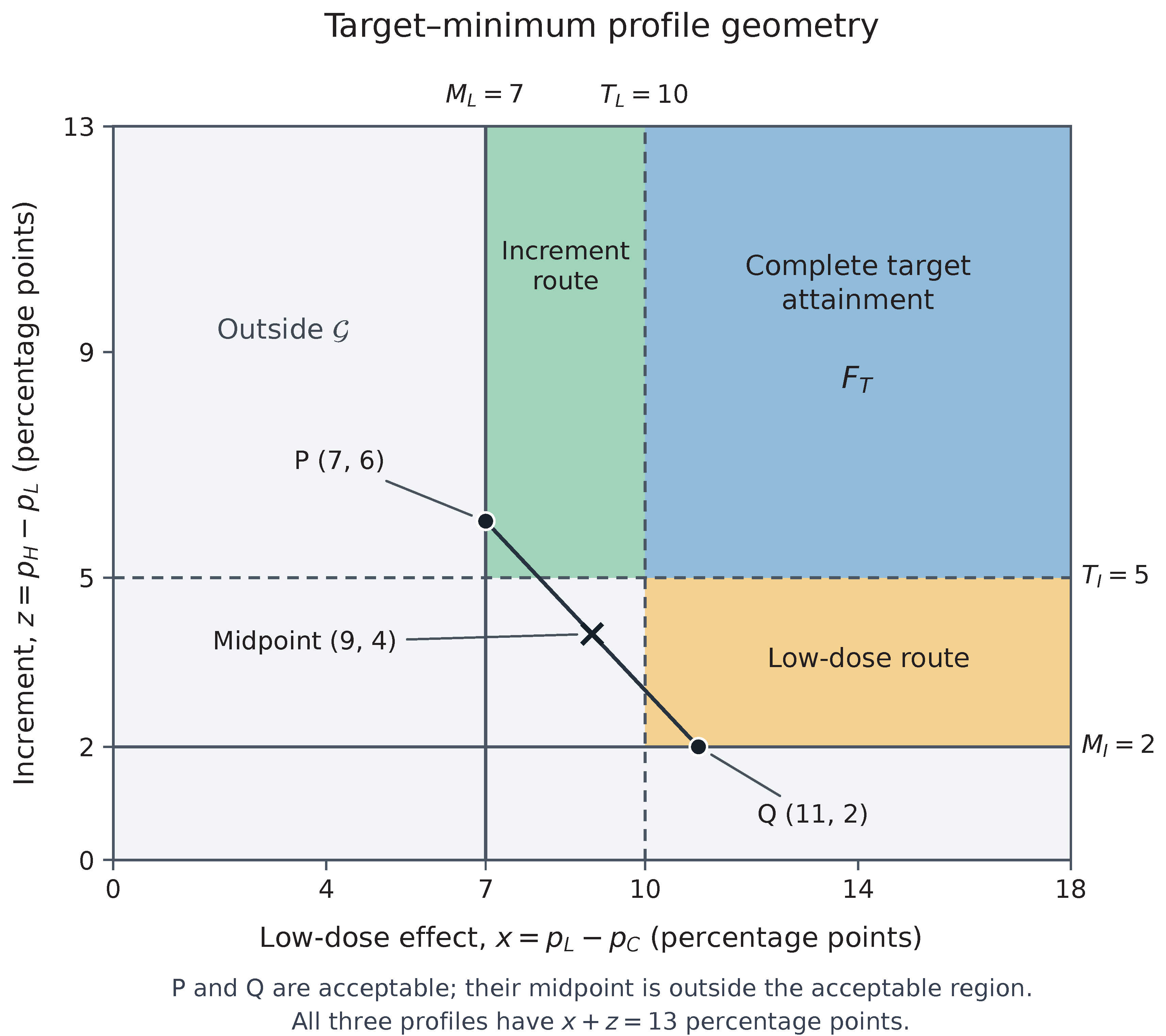
Figure 2.
A. D250, with . Route L exceeds only the low-dose target; route I exceeds only the increment target. The distance is the effect’s excess above its minimum when that effect does not exceed its target; is the other effect’s excess above its target. Both distances are in percentage points. Filled symbols show the power of the certified implemented rules; open diamonds show point-specific upper bounds. The common Figure 2 legend gives the thresholds and calculation details. B. Power and point-specific upper bounds at the specified interior partial-attainment profiles. Panels A and B show D250 and D386 , in control/low-dose/high-dose order, on identical scales. All 24 interior profiles per design exceed both minima and exceed exactly one target. Effects x and z are the low-dose versus control difference and high-dose versus low-dose increment; thresholds are . Filled symbols show power (repeated-trial declaration probability) from finite binomial sums. Joint and componentwise Bayesian rules use independent Beta(1,1) priors; union–intersection/intersection–union (UI–IU) uses W without a prior. All implemented rules have maximal false-declaration probability at most 2.5%. Row labels give control response probability and the route: L exceeds the low-dose target; I exceeds the increment target. Boundary distances are , for L, and , for I, in percentage points. Open diamonds show the smaller of the two one-group Neyman–Pearson upper bounds: a power ceiling, not an achieved rate. This ceiling need not be attainable under the full null. Figure S6.1 enlarges rates; S5.8 gives the sharper two-group bound for the specified D386 profile.
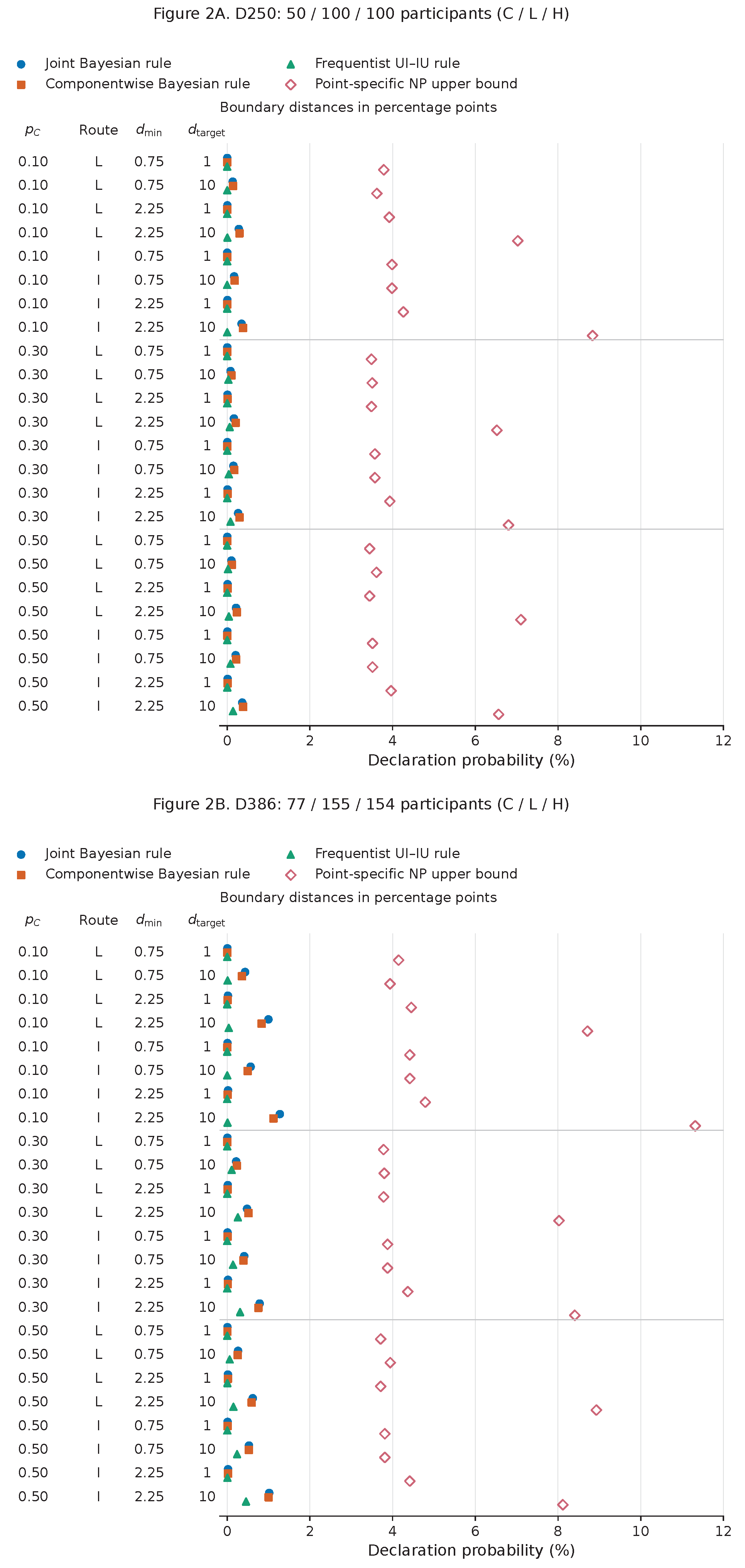
Figure 3.
Posterior attainment states and expected target shortfalls in the JADE MONO-2 illustration. Published responder counts [12] are with denominators , in placebo, abrocitinib 100 mg and abrocitinib 200 mg order. The effects x and z are the low-dose versus control difference and high-dose versus low-dose increment. Their illustrative minimum and target thresholds are . A: Entries are posterior probabilities in percent under independent Beta(1,1) priors. Rows classify x and columns classify z as below minimum, from minimum through target inclusive, or above target. Thick borders identify the three acceptable cells: both minima are met and at least one target is exceeded. Cells below 0.001% are labelled accordingly; full-precision values are retained in Data S1. Threshold labels are effect sizes in percentage points. B: Posterior means of and in percentage points under independent Beta(1,1) and Beta(1/2,1/2) priors. The positive part assigns the deficit below a target when the effect is deficient and zero when the target is reached or exceeded. Each expectation therefore averages over the entire posterior, rather than only deficient profiles. Values smaller than 0.001 percentage points are labelled accordingly.
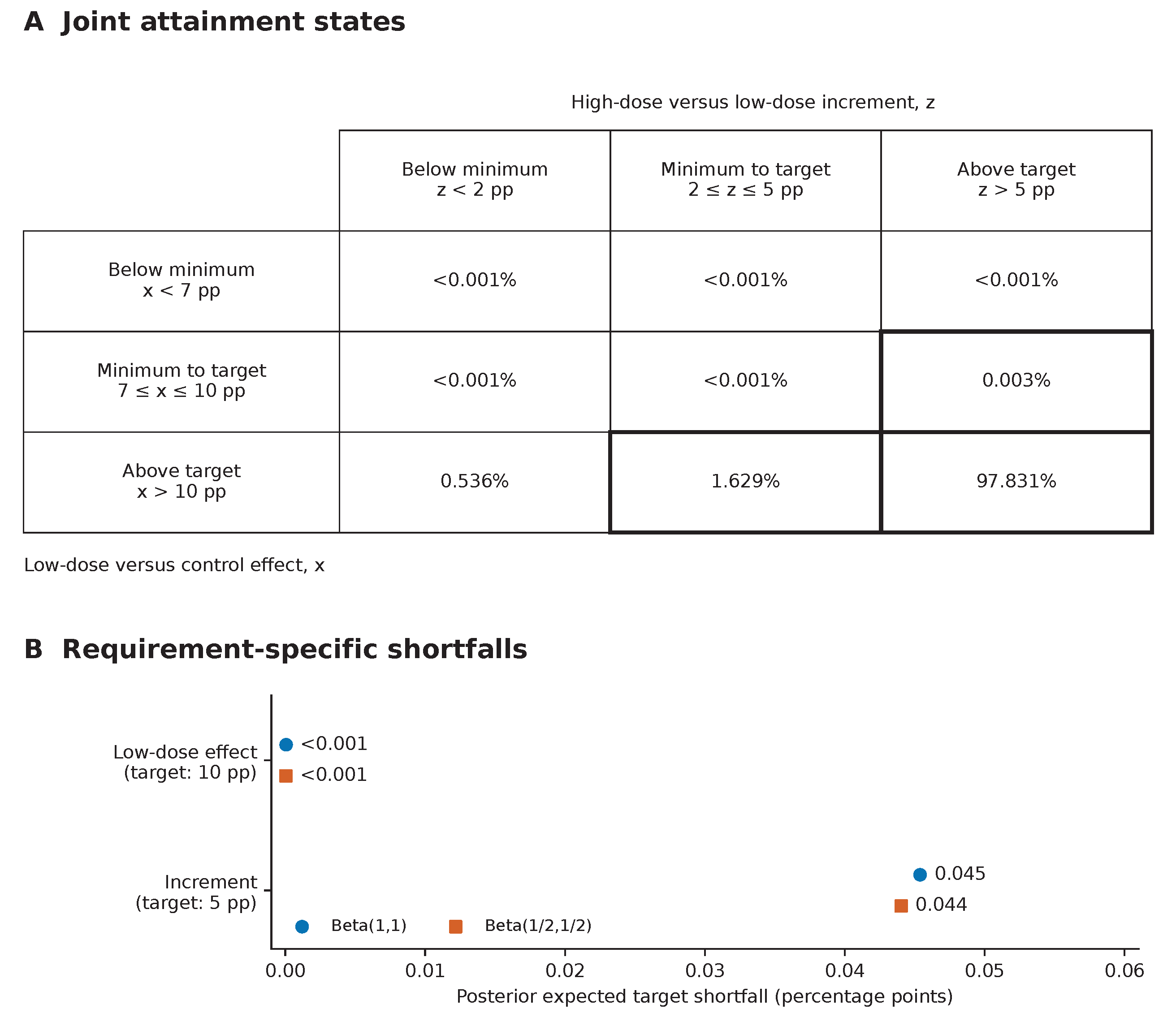
Table 1.
Method-independent declaration-probability bounds on the increment-route slice at .
| Low-dose sample size | Upper bound (%, rounded) |
| 100 | 9.08 |
| 200 | 14.00 |
| 500 | 28.25 |
| 1,000 | 49.77 |
Values are evaluations of for , rounded to the nearest 0.01 percentage point rather than rounded upward. They cover every feasible profile with , and , for any positive fixed control and high-dose denominators. They are not achieved declaration probabilities.
Table 3.
Calibration of the six primary implemented decision rules.
| Design | Rule | Implemented cutoff | Error upper bound (%) | Path | Calib. (s) |
| D250 | > 0.976140 | ≤2.4694 | 9.82 | ||
| D250 | > 0.976140 | ≤2.4694 | 8.68 | ||
| D250 | ≤ 0.027602 | ≤2.1029 | 5.98 | ||
| D386 | > 0.976110 | ≤2.4951 | 74.86 | ||
| D386 | > 0.976110 | ≤2.4951 | 72.84 | ||
| D386 | ≤ 0.025045 | ≤2.4949 | 57.02 |
, and denote the implemented scores for the joint Bayesian, componentwise Bayesian and frequentist UI–IU rules, respectively (Section 5.1). A tilde identifies a numerical score used to construct the saved decision table. The two Bayesian rules use independent Beta priors; uses no prior. All six rules address the same and error limit . Reported error bounds are conservative upper bounds for the maximum false-declaration probability over the full composite null; they are rounded upwards to four decimal places and are not confidence limits. Cutoffs are rounded to six decimal places for display only; archived integer ticks and boundary tables define the decisions. “Path” identifies the path attaining the largest false-declaration probability; and correspond to failure of the low-dose and increment minima, respectively, including their limiting boundaries (Section 4.2). Times cover cutoff calibration and certification only. Full calibration summaries are given in S6.2 and S6.8. Guarantees apply to the archived decision tables; at the archived full-precision D386 joint cutoff, the corresponding ideal posterior rule exceeds the error limit at a strict null point (S4.8).
Table 4.
Published trial summaries and target–minimum assessment for JADE MONO-2.
| A. Published trial data | |||
|---|---|---|---|
| Group | Responders/denominator | Observed response (%) | Randomized N |
| C: placebo | 8/77 | 10.39 | 78 |
| L: 100 mg | 69/155 | 44.52 | 158 |
| H: 200 mg | 94/154 | 61.04 | 155 |
| B. Posterior probabilities under independent Beta(1,1) priors | |||
| Event | Probability (%) | ||
| Acceptable profile, | 99.46 | ||
| Complete target attainment, | 97.83 | ||
| Low-dose route only, | 1.63 | ||
| Increment route only, | 0.003 | ||
| Outside | 0.54 | ||
| C. Application of the saved D386 joint-rule table | |||
| Implemented score (0–1 scale) | 0.9946 | ||
| Cutoff (strict >; score scale) | 0.9761 | ||
| High-dose responses required at | 90 | ||
| Published high-dose responder count | 94 | ||
| Illustrative joint declaration | Yes | ||
EASI-75 denotes at least 75% improvement from baseline in the Eczema Area and Severity Index. The low-dose route exceeds only the low-dose target while meeting the increment minimum; the increment route exceeds only the increment target while meeting the low-dose minimum. The published week-12 EASI-75 summaries [12] are used as fixed binomial inputs; analysis denominators are not replaced by randomized totals. The illustrative thresholds are . Posterior probabilities in panel B are percentages; score and cutoff in panel C are on the 0–1 scale and are rounded for display. The three acceptable-state probabilities sum to before display rounding. The rule is applied through the saved integer boundary table, not rounded printed probabilities. For this saved table under the stated binomial model, the maximal false-declaration probability is bounded by 2.4951% (rounded upwards; Table 3).
Disclaimer/Publisher’s Note: The statements, opinions and data contained in all publications are solely those of the individual author(s) and contributor(s) and not of MDPI and/or the editor(s). MDPI and/or the editor(s) disclaim responsibility for any injury to people or property resulting from any ideas, methods, instructions or products referred to in the content. |
© 2026 by the authors. Licensee MDPI, Basel, Switzerland. This article is an open access article distributed under the terms and conditions of the Creative Commons Attribution (CC BY) license (http://creativecommons.org/licenses/by/4.0/).
Copyright: This open access article is published under a Creative Commons CC BY 4.0 license, which permit the free download, distribution, and reuse, provided that the author and preprint are cited in any reuse.