

Submitted:
05 October 2026
Posted:
09 October 2026
You are already at the latest version
Abstract
Native multi-token prediction (MTP) uses a model’s own prediction module to draft future tokens for joint target verification. In hybrid language models, which combine full-attention and recurrent layers, this opportunity faces three coupled constraints: uneven numbers of accepted tokens, duplicated candidate states, and dependencies that limit verification parallelism. We present Xtra-MTP, which jointly designs candidate coverage, recoverable state, and Gated DeltaNet execution. One-token alternatives extend one recursively drafted path without recursively expanding additional branches. A shared checkpoint and compact update records preserve candidate continuations; the next verifier recovers only the selected path, sharing state access with verification. A topology-aware solver separates updates that propagate along the path from terminal readouts, while value tiling exposes parallel execution. Across three Qwen models and six workloads, with the 95th percentile of request average time per output token (TPOT) constrained to 30 ms, measured configurations improve six workload geometric-mean throughput by 29.4–39.2% over the best tested SGLang configurations and 5.9–9.2% over our ReplaySSM integration.
Keywords:
speculative decoding
; native multi-token prediction
; hybrid attention
; state-efficient verification
; parallel verification
; gated DeltaNet
; LLM serving
1. Introduction
Native multi-token prediction (MTP) modules in models such as DeepSeek-V4 and Qwen3.5 draft future tokens without additional draft-model training (DeepSeek-AI 2026,Qwen Team 2026). The target model jointly verifies these candidates and selects a continuation (Leviathan et al. 2023). This parallelism within a request complements batching across requests, which improves hardware utilization but can lengthen decoding steps (Agrawal et al. 2024). When accepted drafts amortize the extra work, speculation can raise throughput at a given request latency or reduce latency at a given throughput (Sadhukhan et al. 2025).
Hybrid language models interleave full attention with recurrent layers, such as Qwen3.5’s Gated DeltaNet (GDN) (Qwen Team 2026). Full attention retains token-indexed key-value (KV) entries; GDN summarizes the consumed prefix in a fixed-size state. Each candidate depends on its ancestors’ state updates, and the selected continuation must remain recoverable. Our measurements reveal three coupled serving bottlenecks (Figure 1).
First, median latency gains need not extend to tail requests. A chain accepts drafts only up to its first mismatch. On MT-Bench with Qwen3.8-27B-FP8, depth seven and 16 concurrent requests, native MTP reduces median time per output token (TPOT) by 32.5% versus autoregressive decoding, but p95 by just 3.9%; p99 increases 2.8%. These are percentiles of request-average TPOT. Second, candidate states consume concurrency capacity. At 32 allocated slots, Qwen3.5-4B’s candidate GDN storage grows from 6 to 24 GiB as depth rises from three to fifteen. Such duplication can limit the batch that fits before throughput saturates. Third, recurrent dependencies constrain parallel verification. At batch 32, depth fifteen and a 256-token prefix, target-only verification speedup reaches 8.12× for Qwen3-4B but 3.95× for Qwen3.5-4B.
Existing methods already address several of these costs. ReplaySSM uses compact history, deferred state write-back and a triangular GDN solve (Dao AI Lab 2026). Concurrent Bole combines factorized tree verification, selected-state reconstruction, value tiling and hardware-aware candidate budgets (Wang et al. 2026). We investigate a specific design for small native-MTP budgets: terminal candidates that need no recursive continuation, a solver exploiting that structure, and selected-state recovery sharing the next verifier’s state access.
Xtra-MTP separates candidate output computation from reconstruction of the selected state matrix. Its three contributions address Challenges 1–3:
- C1: Budgeted terminal coverage. To improve coverage without recursive widening, we retain terminal alternatives from the distributions along one primary draft path (the spine). Reach-weighted placement allocates a limited leaf budget; profiling selects between a chain and one-token alternatives at each serving operating point.
- C2: Consumer-coupled state recovery. To avoid per-candidate matrices, we preserve continuations with a shared checkpoint and compact update records. Recovery runs inside the next verifier that needs the selected state, avoiding an intermediate matrix handoff and permitting record storage to be reused across rounds.
- C3: Topology-aware parallel GDN execution. To expose candidate parallelism, a spine-first solve computes the updates that descendants need; terminal leaves consume them without propagating further. Tiling across requests, heads and value dimensions parallelizes readout and recovery.
Across three Qwen models and six workloads, measured configurations improve geometric-mean throughput under a 30 ms request-p95 TPOT budget by 29.4–39.2% over SGLang and 5.9–9.2% over our ReplaySSM integration. Task-balanced regression gives up to 64.5% higher throughput at matched p95 and 57.9% lower p95 at matched throughput versus SGLang; Section 5 reports both fitted and measured comparisons.
2. Background and Verification Bottlenecks
2.1. Native MTP and Recurrent Continuation
A speculative round drafts candidates, verifies target outputs and selects a continuation. Its spine is the primary recursively drafted path of D tokens. The root is already target-selected and is consumed at this round’s start. Adding E terminal leaves gives verified nodes; is a chain. H1 denotes one-token side branches (length ), regardless of leaf count. Native beam2 recursively expands two continuations per step before pruning for verification. Accepted progress a counts accepted drafts, excluding the root and target-selected bonus token that becomes the next root.
Candidate topology is the parent/branch structure; coverage is its ability to retain target-compatible continuations. Budgets bound depth and additional candidates. We distinguish active GPU batch B, client concurrency C and allocated request slots P. GDN updates a prefix summary from projected inputs and gates ; state recovery follows the selected candidate’s ancestor path.
2.2. Candidate Coverage and Uneven Progress
Figure 1a shows that median gains need not extend to tail requests. Native MTP D7 reduces MT-Bench median TPOT by 32.5%, p95 by 3.9%, and raises p99 by 2.8%; Alpaca p99 rises 1.1%. Here p50/p95/p99 are percentiles across request averages. Early mismatch leaves fewer accepted drafts to amortize drafting and verification. Section 3.1 tests whether extra coverage justifies its cost.

2.3. Candidate-State Duplication
At , Qwen3.5-4B requires 6/12/24 GiB of candidate GDN states for D3/D7/D15, versus 13.18 GiB for weights plus two 128K-token KV pools (Figure 1b). This buffer accounting follows : is the recurrent layer count, s the state bytes per layer, and the allocated candidate capacity per slot, beyond committed states. Duplication can consume memory needed for more requests before compute throughput saturates.

2.4. Recurrent Dependencies Limit Parallel Verification
At , prefix length , target-only speedup is 8.12× for Qwen3-4B and 3.95× for Qwen3.5-4B (Figure 1c). For chain nodes,
Both times include target outputs and state writes. This compares verification amortization within each model. GDN’s ancestor-dependent updates admit parallel formulations (Yang et al. 2025); exploiting them requires reorganizing candidate computation.

3. Design Principles and Controlled Analysis
Contributions C1–C3 address coverage, state storage and execution in the order of Challenges 1–3. Candidate controls match target prefixes; GDN controls match operands, topology and selected paths. GDN lifecycle time covers verification, selection, record maintenance and amortized final state reconstruction. It excludes upstream query/key/value (QKV) and gate projections, convolution, feed-forward networks (FFNs), drafting and sampling. Appendix A specifies the cohorts.
3.1. Budgeted Terminal Coverage
C1 seeks useful coverage without recursively expanding multiple draft continuations (recursive widening). Xtra retains one-token alternatives from distributions already computed along one spine. A matching terminal leaf rescues one token without drafting another continuation or reconnecting the unused spine suffix. In the D7 control, chain/H1 use six recursive MTP rows versus beam2’s twelve, verifying 8/9 versus 15 nodes.
Let be the full-vocabulary-normalized draft probability of rank j at position i. For the deployed one-leaf profile (), global allocation chooses
This reach-weighted draft score places the leaf; target verification determines acceptance. A fork budget F caps distinct branching parents; the serving profile uses . Chain () and Global H1 use the same implementation, with the profile fixed for each serving run.
Placement matters: 251 of 308 potential top-2 rescues (81.5%) in the 27B/D7 trace occur after position one (Figure 2a). On 191 matched 4B/D7 first-output prefixes, global H1 captures 25.6% of beam2’s mean accepted-length increment over chain using 12.4% of its additional projection work (Figure 2b). Root H1 more directly reduces zero acceptance, whereas global placement improves mean progress (Appendix C.4).
At low concurrency, terminal coverage can amortize verification over more outputs. On MT-Bench D3/ (Figure 3), H1 lowers request-p95 TPOT relative to Xtra chain by 4.8/6.0/1.7% for 4B/27B/35B-A3B. On 27B, the median falls 4.4% and measured throughput rises 4.1%. On 35B, H1’s median rises 2.6% despite its lower p95. SGLang beam2 narrows its relative tail but raises 35B latency. Appendix C.10.10.11 separates absolute latency from median-normalized tail spread.
Extra verification limits high-concurrency gains: on 4B/GSM8K/D7 at , H1 retains 95.2% of Xtra chain throughput, versus 67.4% for beam2 relative to SGLang chain (Figure 2c). Offline profiling chooses chain or H1 for each operating point; draft probabilities determine leaf positions. Appendix C.4 details the execution costs.
3.2. Consumer-Coupled State Recovery
C2 separates compact representation from recovery timing. Let be the per-head key/value dimensions and their head counts. For a GDN state , normalized key , value v, log-decay g and update strength (Yang et al. 2025),
A post-root checkpoint stores the state after consuming . The raw journal holds candidate operands ; a selected-path cursor identifies the endpoint to recover. This representation is lossless in real arithmetic and reduces per-head storage from SGLang’s matrices to . Materialization reconstructs the full matrix from the checkpoint and selected records, costing per head. Derivations and validation appear in Appendices Appendix C and Appendix C.5.
Vector-sized records also appear in Bole and ReplaySSM (Dao AI Lab 2026,Wang et al. 2026). Xtra couples recovery to its next consumer, the verifier needing the selected state, and reuses one journal. At , peak CUDA-allocator memory is 36.36 MiB versus 291.02 MiB for SGLang (8.0× smaller) and 36.55 MiB for ReplaySSM (Figure 4a). The journal stores raw operands; solved residuals remain transient.
With raw-record representation and verifier tiles fixed, deferring recovery to the next verifier reduces mixed-trace lifecycle time by 3.6/24.5% for , including final materialization (Figure 4b). Geometry and selected length affect gains; eager recovery is faster at full acceptance for (Appendix C.3).
3.3. Topology-Aware Parallel GDN Execution
C3 exploits the distinction between spine nodes, whose updates propagate, and terminal leaves, which only consume ancestor updates. Expanding the recurrence around the checkpoint moves dependencies from full matrices to residual vectors. Blocked checkpoint projections and readout surround an ancestry-constrained solve. For spine candidates c and terminal leaves ℓ,
where R contains checkpoint-relative updates and A their weighted ancestry interactions. Xtra solves spine columns first. Leaves consume these residuals without becoming propagation sources.
On matched inputs and paths, Xtra’s GDN lifecycle is 1.68–1.98× faster than ReplaySSM at , D3/D7/D15 (Figure 4c). Replacing its solver with the finite Neumann-series solver used in our Bole reproduction (Wang et al. 2026), retaining the other components, increases D7 lifecycle time by 6.2–8.1% across (Figure 4d).
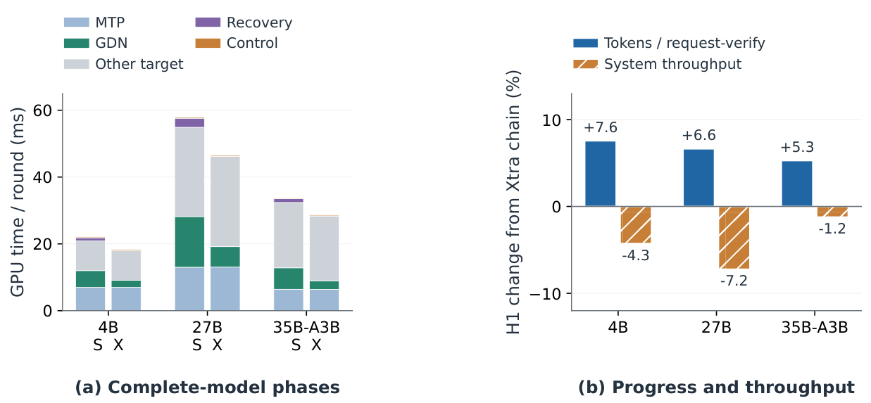
Each execution unit owns one request, value head and value tile of width , exposing independent units. Removing value tiling at the same total warp budget raises B16/D7 lifecycle time by 48.7%. A terminal leaf adds 6.5–7.1% within the tested D7 tile extent; padding boundaries change this cost (Appendix C.3). Complete-model profiles retain substantial MTP and non-GDN work, limiting how much layer speedup reaches serving throughput (Appendix C.4).
4. Cross-Round Integration
The three mechanisms form a serving lifecycle when the next round can consume the selected continuation. Xtra coordinates candidate parents, logical state and storage ownership across that boundary (Figure 5).
4.1. Output Computation and Logical Continuation
The post-root checkpoint , journal records and selected endpoint represent the consumed prefix as
Here is the root-to-endpoint path and Fold applies Equation 3 in that order. Target selection fixes without immediately writing its matrix. For , the continuation contains and excludes the unused spine suffix. Its matrix is materialized when the next consumer needs it.
4.2. Fused Recovery and Safe Journal Reuse
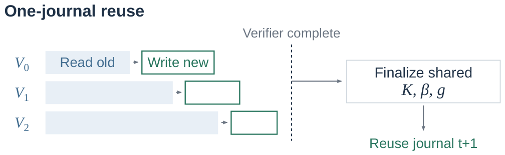
Each request–head–value-tile owner folds the previous suffix, absorbs the new root, projects the checkpoint, solves residuals and reads out candidates. Recovery shares state access with verification, removing the intermediate write and reload of the recovered matrix.
An owner may overwrite its private value records after their last read. Keys and gates serve multiple owners, so a following kernel on the same CUDA stream replaces them after all verifier programs finish. The new journal survives target selection and supplies the next selected suffix. This ordering permits value parallelism with one journal; Appendix C.2 proves the cross-round invariant.
4.2.0.1. Serving integration.
The selected endpoint coordinates GDN recovery, convolution windows, full-attention KV selection and MTP refresh. Each component represents the same logical consumed prefix, even when the GDN matrix awaits materialization. Integration with SGLang (Zheng et al. 2024) uses GPU metadata and fixed-capacity buffers to preserve CUDA Graph addresses and shapes. Parent masks coordinate packed chain/tree attention and GDN execution. External readers materialize pending state before consuming it; Appendix C.2 records the lifecycle transitions. Chain and H1 share this lifecycle. Offline profiling fixes the budget for each model, workload, depth and concurrency; per-request probabilities control leaf placement within that budget.
5. Evaluation
We evaluate throughput–latency trade-offs, then memory-budget throughput, testing the complete-model value of Section 3’s mechanisms.
5.1. Experimental Setup
We use Qwen3.5-4B (Qwen Team 2026), Qwen3.8-27B-FP8 ( ) and Qwen3.6-35B-A3B-FP8 ( ) on H100 PCIe 80 GiB GPUs, with native MTP and the named precision (FP8: 8-bit floating point). GDN keys/values use bfloat16 (BF16), checkpoints 32-bit floating point (FP32). Xtra’s BF16x3 checkpoint projections sum three BF16 matrix products with FP32 accumulation (Appendix C.1). Workloads are MT-Bench (Zheng et al. 2023), Alpaca (Taori et al. 2023), GSM8K (Cobbe et al. 2021), MATH-500 (Lightman et al. 2023,Hendrycks et al. 2021), HumanEval (Chen et al. 2021) and LiveCodeBench (Jain et al. 2024).
Baselines are SGLang based on source revision fd19a762, our raw-operand/reference-order ReplaySSM port and our Bole reproduction (Dao AI Lab 2026,Wang et al. 2026,Zheng et al. 2024). All methods use this SGLang serving revision; Appendix A.1 details the source pins and integrations, including how our ReplaySSM port differs from its published correction-vector/deferred-write-back variant. We evaluate SGLang/Bole with chain and beam2, and ReplaySSM with chain. One frozen Xtra implementation supports chain and Global H1 (). Offline profiling selects the higher-throughput chain/H1 run for each model/workload/depth/concurrency in fitted summaries, preserving paired latency. Budgeted comparisons search all eligible configurations. We test and with one process per cell. Prompts and capacities match within each workload; greedy generation produces 512 tokens with early end-of-sequence (EOS) and prefix caching disabled. The compact state representation preserves the recurrence in real arithmetic; Appendix C.5 reports floating-point validation of the frozen implementation.
Throughput covers the complete measured stage, including prefill, fill/drain and final materialization. Request latency is
where and are the first/last output times and the output count. Request-p95 is the 95th percentile of these averages. Each budgeted comparison selects the highest observed throughput over D3/D7, tested concurrency and supported topologies within each workload. All metrics come from that qualifying run; six-task summaries use geometric means. Appendix A records sample counts and implementation details.
5.2. Throughput–Latency Trade-Offs
5.2.0.2. Fitted trade-offs.
Figure 6 summarizes throughput and request-p95 TPOT across six workloads using 1,554 selected runs, with throughput and latency paired within each run. Gaussian-kernel regression fits give each workload equal total weight. At matched request-p95 TPOT, the fitted curves show maximum throughput gains of 64.5/53.4/61.2% over SGLang for 4B/27B/35B-A3B. At matched fitted throughput, maximum p95 reductions are 57.9/34.5/44.8%. These maxima can occur at different operating points. The curves describe configuration trends; Appendix A.3 specifies selection, fitting and comparison domains.
5.2.0.3. Measured configurations under latency budgets.
Figure 7 complements the fits with per-workload throughput under a 30 ms request-p95 budget, retaining SGLang/Bole chain and beam2 separately. Xtra’s gains over the better SGLang topology range from 17.8% to 68.4% across the 18 model–workload pairs. Its six-workload geometric-mean throughput gains over SGLang’s best tested configurations are 29.4/38.1/39.2% for 4B/27B/35B-A3B. Gains over the fastest baseline, our ReplaySSM integration in every row, are 6.1/5.9/9.2%.
These comparisons evaluate the shared execution backend with candidate budgets configured for the operating point. Section 3.1 shows how H1 complements chain at low concurrency. At fixed D7/ on MT-Bench, Xtra chain improves throughput by 5.0–8.1% over ReplaySSM (Table A4). Appendix B retains the per-topology curves, 20/30/40 ms summaries and configurations, including per-task 20/40 ms comparisons in Appendix B.6.6.9.
5.3. Throughput Under Memory Budgets
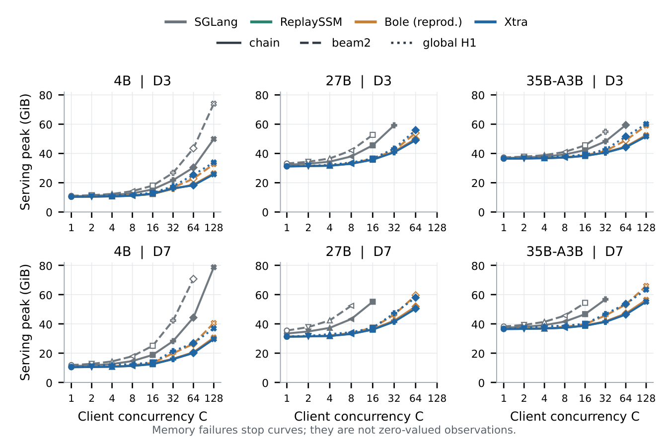
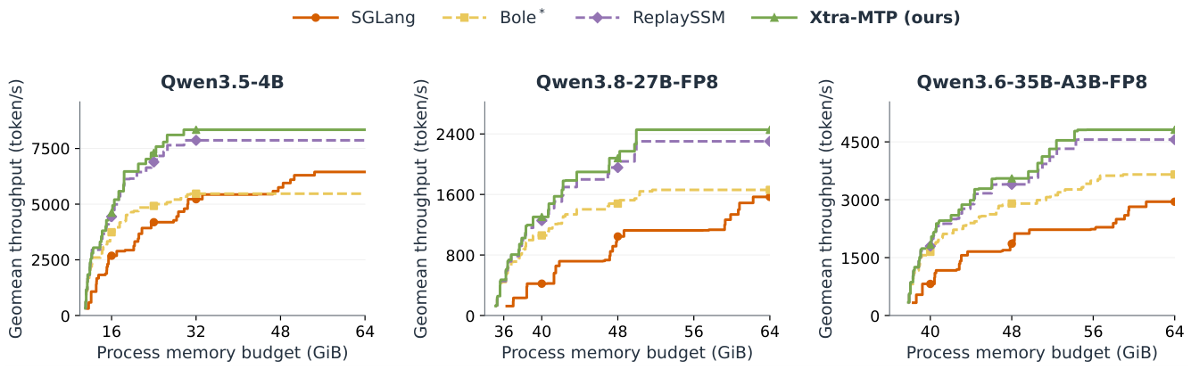
Figure 8 applies a common process-memory budget, sampled with the NVIDIA Management Library (NVML) every 50 ms. Lifetime peaks cover initialization, warmup and serving, with no TPOT constraint. It selects feasible measured runs from the existing sweep. At 24 GiB, 4B reaches 7,306 versus SGLang’s 4,190 token/s (+74.4%). At 48 GiB, gains are 99.1% for 27B and 90.9% for 35B-A3B; gains over ReplaySSM at these budgets are 6.0/6.4/4.5%.
Compressing SGLang’s candidate states enables substantial capacity savings. Against ReplaySSM, total process footprints are close: the matched 4B D7/ serving peaks are both 12.49 GiB, while Xtra’s recovery records are 12.5% smaller. The benefit is higher throughput at a similar footprint. Appendix B.3 provides exact budget values and state accounting.
6. Related Work
6.0.0.4. Candidate generation and verification.
Speculative decoding verifies proposed tokens with a target model (Leviathan et al. 2023,Chen et al. 2023). Tree/head-based proposals (Miao et al. 2024,Cai et al. 2024), feature drafting (Li et al. 2024,Li et al. 2025), and parallel drafting (Chen et al. 2026,Hu et al. 2026) expand candidate coverage. EAGLE-2 and Sequoia adapt candidate trees to confidence or hardware (Li et al. 2024,Chen et al. 2024). Xtra reuses native MTP (Gloeckle et al. 2024), restricts recursive expansion to one spine, and verifies budgeted terminal alternatives.
6.0.0.5. Recurrent-state recovery.
Backtracking/replay and component-aware drafting address speculation in state-space and hybrid models (Wu et al. 2024,Borobia et al. 2026). ReplaySSM combines compact history, deferred write-back and a triangular GDN solve (Dao AI Lab 2026). Concurrent Bole combines factorized tree verification and selected-state reconstruction with value tiling and candidate budgets; TreeWY uses tree-structured WY representations (Wang et al. 2026,Ghantasala 2026). Xtra specializes the dependency solve to one spine with terminal leaves and folds raw selected-path records inside the next verifier’s value-tile owner. Section 5.1 describes our backends.
6.0.0.6. Serving objectives.
DistServe and Sarathi-Serve study latency–throughput trade-offs, while AdaSpec considers serving-aware speculative decoding (Agrawal et al. 2024,Zhong et al. 2024,Huang et al. 2025). Xtra evaluates recurrent verification in SGLang (Zheng et al. 2024) under request-p95 TPOT and process-memory budgets.
7. Conclusions
Xtra-MTP connects budgeted terminal coverage, consumer-coupled state recovery and topology-aware parallel GDN execution. Candidate outputs are verified while full-state recovery follows only the selected path; chain and H1 provide complementary operating points. Across three Qwen models and six workloads, measured configurations under a 30 ms request-p95 TPOT budget improve geometric-mean throughput by 29.4–39.2% over the best tested SGLang configurations and 5.9–9.2% over our ReplaySSM integration. Jointly choosing candidate topology, state representation and execution turns speculative parallelism into serving value.
Appendix A. Evaluation Setup and Reproducibility
Appendix A.1. Environment and Evaluated Implementations
Experiments use H100 PCIe 80 GiB GPUs, tensor-parallel degree one (TP1), and the three Qwen checkpoints and six workloads in Section 5.1. Full models retain their named quantization; GDN operands are BF16 and checkpoints FP32. All serving arms share a locally extended SGLang tree based on fd19a762, native FlashAttention-3 (FA3), fixed CUDA Graph profiles, and disabled prefix caching and overlap scheduling. The implementation manifest pins the full source revisions and executed files by hash.

Table A1.
Evaluated GDN backends and supported serving topologies. Adapter, layout-copy and state-maintenance costs are included.
Table A1.
Evaluated GDN backends and supported serving topologies. Adapter, layout-copy and state-maintenance costs are included.
| Backend | Topologies | Computation and recovery |
|---|---|---|
| SGLang | Chain, beam2 | Native recurrence, full FP32 candidate states and accepted-state scatter. |
| ReplaySSM | Chain | Port of the raw-input ring and reference-order FP32 fold from revision 708f51e4. |
| Bole | Chain, beam2 | Local FP32/IEEE Triton reproduction; finite Neumann-series solve, log-space decays and selected-state reconstruction. |
| Xtra-MTP | Chain, H1 | Frozen balance implementation; BF16x3 projections, FP32 residuals and consumer-side raw-state recovery. |
ReplaySSM denotes the raw-operand/reference-order path, distinct from its correction-vector/ deferred formulation [6]. Bole denotes our reproduction of its ancestry-constrained factorization [7]. Process-local adapters replace GDN verification and selected-state update; native convolution and KV selection retain the same consumed prefix. Appendix C details the integrations. One frozen Xtra implementation supplies all reported results; H1 adds one terminal leaf ().
Appendix A.2. Workloads and Measurement Protocols
Serving uses greedy generation of 512 tokens with early EOS disabled. Throughput includes prefill, fill/drain and final materialization. TPOT statistics are computed across request averages (Equation 6). Repeated prompts at high concurrency extend measurement duration with caching disabled. Table A2 separates independent processes from repeated event windows.
Table A2.
Measurement cohorts. Kernel lifecycle timing covers verification, selection, record maintenance and final materialization; upstream QKV/gate projections, convolution, FFN, drafting and sampling are excluded.
Table A2.
Measurement cohorts. Kernel lifecycle timing covers verification, selection, record maintenance and final materialization; upstream QKV/gate projections, convolution, FFN, drafting and sampling are excluded.
| Study | Inputs and controls | Samples and independent repetitions |
|---|---|---|
| First-prefix coverage | 4B/D7, shared target prefix and spine; MT-Bench, GSM8K, HumanEval | 64 unique prompts/task; 191/192 pass a common two-token agreement screen. Equal task weights. |
| Multi-round placement | Three models, D3/D7, same three tasks; common target prefixes | 16 requests/task, 128-token windows; average rounds per request, then requests and tasks equally. |
| GDN grid / recovery | , , , capacity | 30 windows of 32 rounds/process; three processes at B64/D7, one elsewhere. Recovery: three for mixed , one per fixed length. |
| Execution controls | One layer, shared 17-node fixture; endpoints | Three processes paired by GPU; 30 windows of 32 rounds each. Ranges span process means or paired ratios. |
| Serving sweep | Three models, six tasks, D3/D7; | One process/cell; measured/warmup requests: 160/32 at , 1,920/160 at . |
| Request-TPOT CDFs | Three models, MT-Bench D3/C4; reuse serving-sweep runs and compare four configurations | 160 measured requests, 32 warmups, one process/arm; 512 output tokens. Same ordered prompts within each model. |
| Matched-profile serving | D7/C16, 256-token padded prompts, 16,384 KV tokens; matched Graph/controller | 192 requests (64/task), 16 warmups; one process/arm on the same GPU within each model. |
Auxiliary memory counts unique records/workspaces, excluding the common checkpoint; peak CUDA-allocator memory counts all live allocated buffers. NVML samples process memory every 50 ms. Lifetime peaks include initialization, warmup and serving; stage peaks cover serving alone. Shorter transients may be missed. Request/KV capacities match within each comparison, with context limit 8,192 and memory fraction 0.85. MT-Bench D7/C16 reserves 20,992 KV tokens for 4B/35B-A3B and 23,296 for 27B; C64 uses 83,200/93,184. Of 2,016 supported sweep cells, 1,830 succeed, 162 fail for memory and 24 inherit resource refusals; ReplaySSM beam2 is unsupported.
Appendix A.2.2.7. Motivation cohorts.
Figure 1c uses BF16 execution, FP32 states, FA3 and Triton GDN: 300 verify samples and 600 bracketing decode samples per point. Qwen3-4B/30B use Instruct-2507; one cross-GPU decode bracket differs by less than 0.1% from its same-GPU check. Panel (a) uses 27B-FP8/C16, 32 warmups and 160 requests/task/method, combining historical MTP with newer AR runs. Full six-model efficiency, buffer accounting and raw quantiles remain in the indexed supplementary data.
Appendix A.2.2.8. Request-distribution cohort.
The MT-Bench CDFs reuse complete serving-sweep runs selected after screening 276 matched H1/chain pairs. Every arm uses the same ordered prompts; event-derived TPOT agrees with the run summaries. Xtra chain/H1 pairs share a physical GPU. SGLang uses another H100 for 4B/27B and the same GPU for 35B. The source index retains GPU identities and request-log hashes. Curves count requests on 513 shared thresholds; table quantiles use the unbinned timings. The distribution is across request averages.
Appendix A.3. Aggregation, Fitting and Reproduction
Xtra exposes chain and Global H1 as candidate-budget configurations of the same implementation. At each profiled model, workload, depth and concurrency, the regression views retain the higher-throughput complete run: 200 chain and 76 H1 runs alongside 1,278 baseline runs. Offline selection preserves each run’s paired throughput and latency and represents its configured operating point. Each task has fit weight , split equally among its configurations. Gaussian-kernel regression uses an unpenalized intercept, length scale 0.55 of each series’ observed latency range and normalized ridge 0.001, with no Pareto filtering or extrapolation. Mean, p50, p95 and p99 describe TPOT within each run; requests are not pooled across tasks.
Fitted throughput annotations maximize the Xtra/baseline ratio over the latter half of common observed latency. Fitted latency reductions maximize over common fitted throughput, taking each curve’s lowest-latency crossing. These separate extrema can occur at different curve locations. Coordinates, fit parameters and the original p95 length-scale sensitivity are retained in the artifact.
For eligible runs of model m, workload w and method s, the latency- and memory-budget summaries use
where is throughput, is request-p95 TPOT, and is sampled lifetime process-memory peak. L and M are the latency and memory budgets. Selection uses unrounded values and each winning run’s complete metrics; six-task summaries are geometric means. SGLang best searches chain and beam2. Memory curves test every observed threshold without interpolation, showing a method only when all six tasks are feasible. These are maxima over the measured configuration grid, not capacity searches or sustainable arrival-rate measurements.
The reproduction index links source/input manifests, numerical checks, and kernel and serving summaries. Compact run tables, selected configurations and fitted coordinates are included; bulk traces are retained separately.
Appendix B. Complete Evaluation Results
Appendix B.1. Multi-Metric Throughput–Latency Summaries
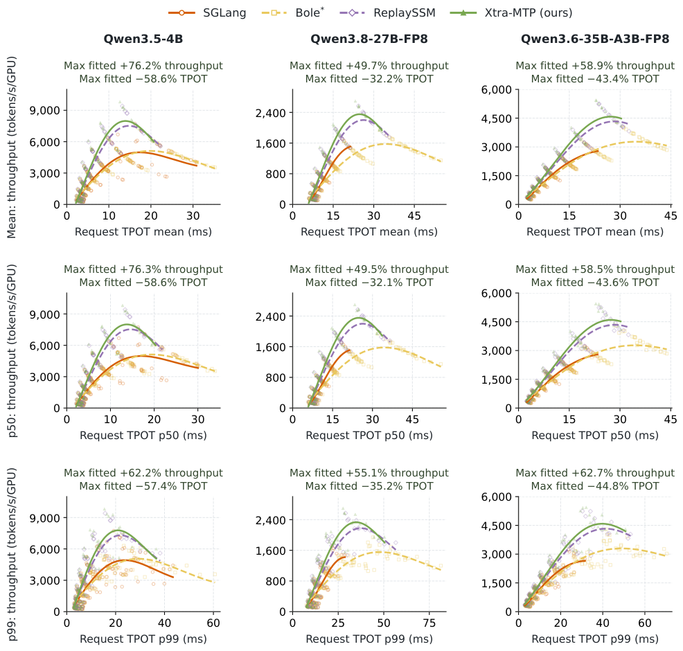
Figure A1 uses the same 1,554 selected runs and 1,093,440 measured requests as the main p95 view, changing only the request-TPOT statistic. Mean and median fits are similar; the p99 views extend to higher latency and yield different comparison extrema. Annotations follow Appendix A.3; the measured curves below retain individual workloads and topologies.
Figure A1.
Six-workload throughput versus mean, p50 and p99 request TPOT. Points are measured runs; fits weight tasks equally. Annotations are separate maximum fitted throughput gains and TPOT reductions versus SGLang on common support. Columns share y-axis scales across statistics; x-axis scales follow each statistic’s observed range. Bole is our reproduction.
Figure A1.
Six-workload throughput versus mean, p50 and p99 request TPOT. Points are measured runs; fits weight tasks equally. Annotations are separate maximum fitted throughput gains and TPOT reductions versus SGLang on common support. Columns share y-axis scales across statistics; x-axis scales follow each statistic’s observed range. Bole is our reproduction.
Appendix B.2. Per-Workload Measured P95 Curves
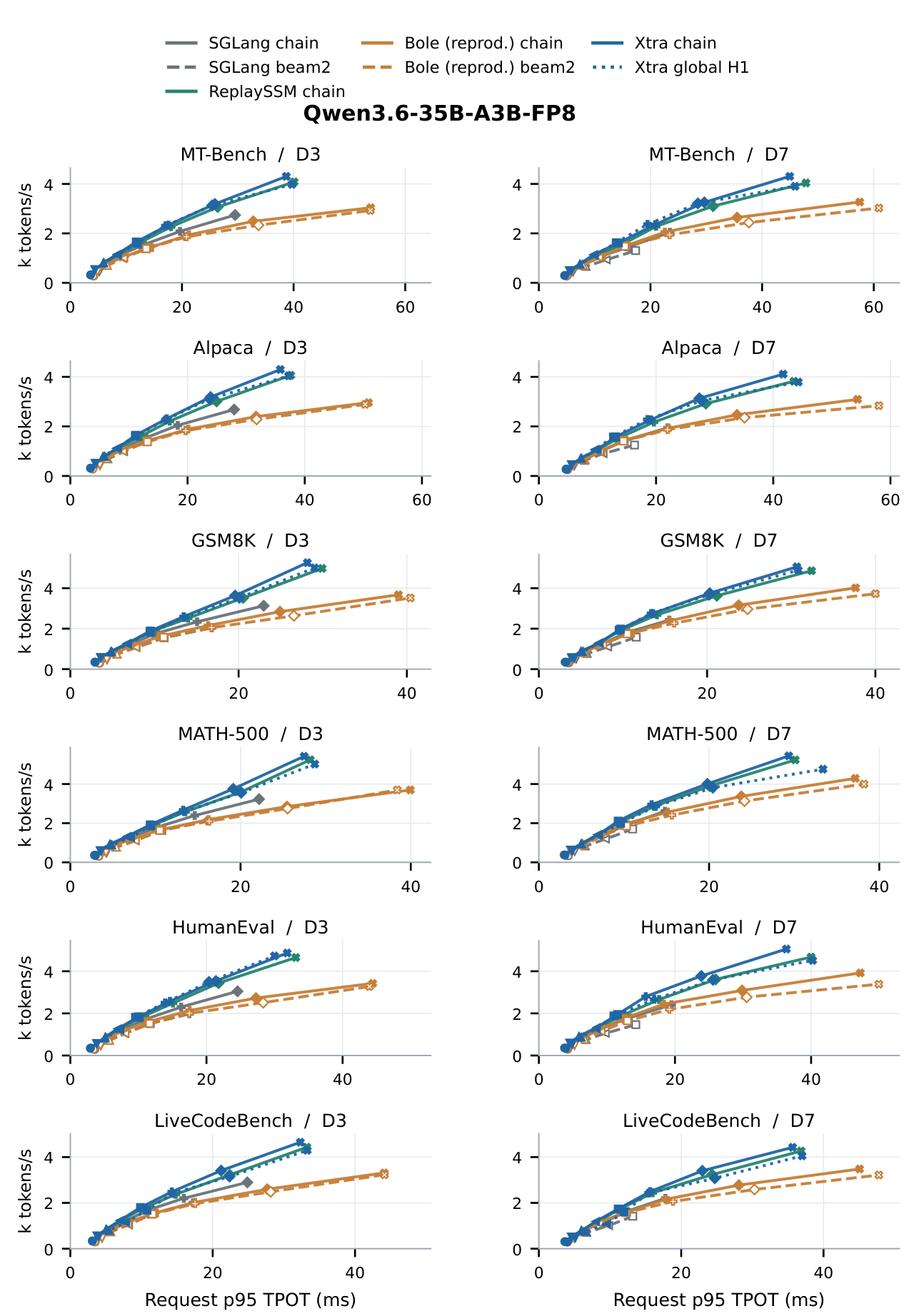
Figure A2–Figure A4 connect valid runs in concurrency order, , at fixed backend, topology and depth. D3/D7 axes match within each task; resource failures leave gaps. Xtra chain and H1 remain separate.
Figure A2.
Qwen3.5-4B: measured throughput–p95 curves for six tasks and D3/D7. Solid/dashed/dotted denote chain/beam2/H1; colors identify backends. Each point is one process under Table A2.
Figure A2.
Qwen3.5-4B: measured throughput–p95 curves for six tasks and D3/D7. Solid/dashed/dotted denote chain/beam2/H1; colors identify backends. Each point is one process under Table A2.
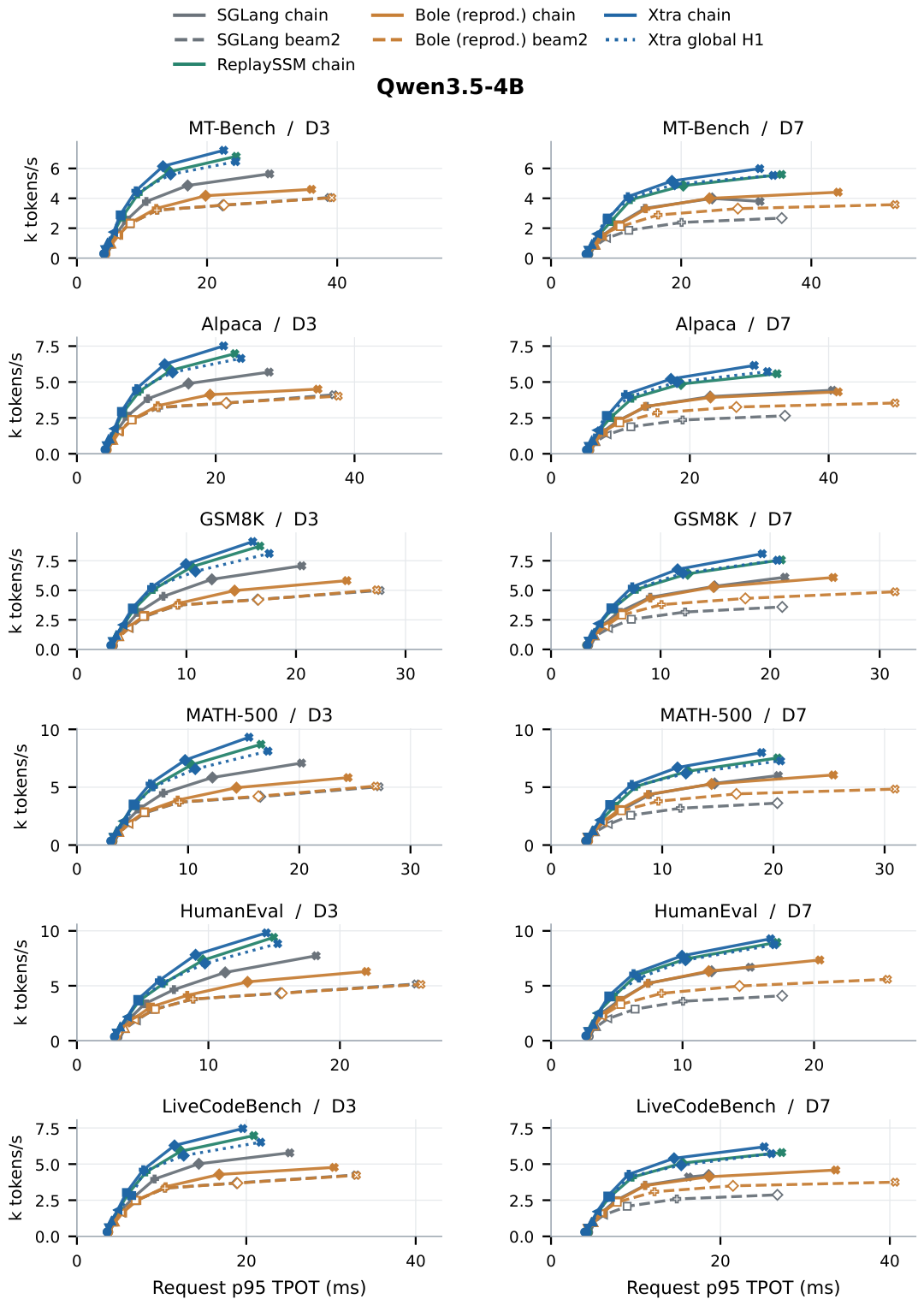
Figure A3.
Qwen3.8-27B-FP8: six tasks and D3/D7, with the encodings and protocol of Figure A2. Resource failures terminate the corresponding curve.
Figure A3.
Qwen3.8-27B-FP8: six tasks and D3/D7, with the encodings and protocol of Figure A2. Resource failures terminate the corresponding curve.
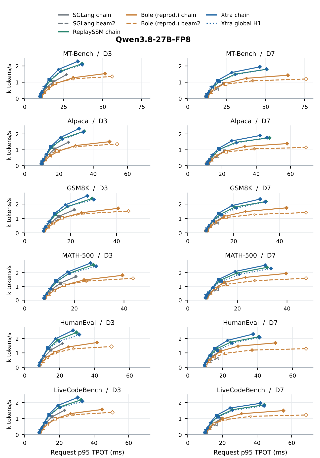
Figure A4.
Qwen3.6-35B-A3B-FP8: six tasks and D3/D7, with the encodings and protocol of Figure A2.
Figure A4.
Qwen3.6-35B-A3B-FP8: six tasks and D3/D7, with the encodings and protocol of Figure A2.
Appendix B.3. Budgeted Results and Fixed-Configuration Controls
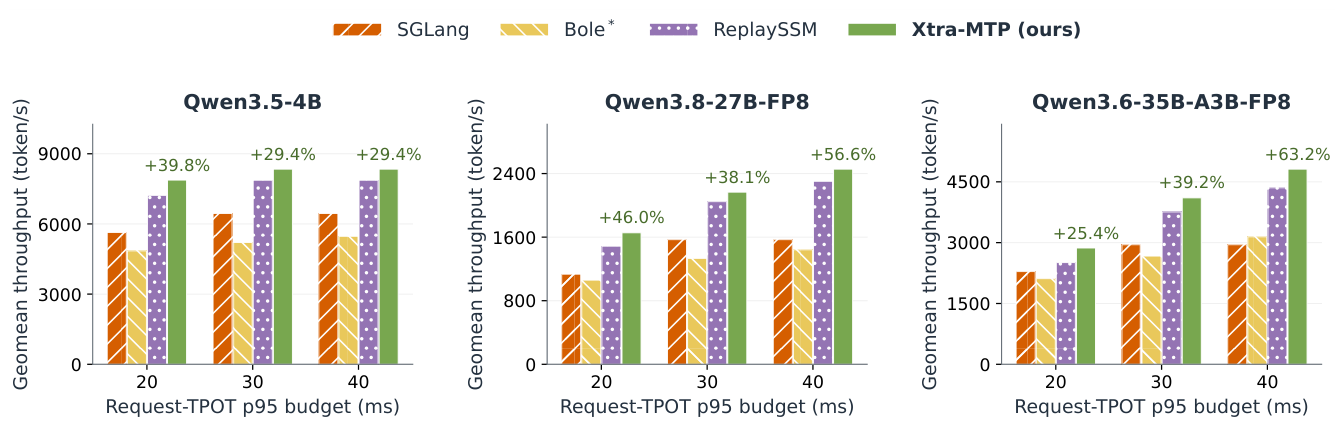
Figure A5 summarizes 20/30/40 ms budgets. Table A3 gives per-task 30 ms results; Table A4 fixes D7/C64. Table A5 gives memory-budget values and Figure A8 shows concurrency scaling; state/process components are in Table A6.
The 30 ms Xtra winners select chain in 17 cells and H1 in one; ReplaySSM is the fastest baseline in all 18. The 35B HumanEval winner’s p95 is 29.982 ms. The manifest records each winner’s configuration, latency and run ID.
Figure A5.
Maximum observed throughput under request-TPOT p95 budgets: geometric means of six per-workload maxima. Labels give gains over SGLang; Bole is our reproduction. Panels use separate y-axis scales.
Figure A5.
Maximum observed throughput under request-TPOT p95 budgets: geometric means of six per-workload maxima. Labels give gains over SGLang; Bole is our reproduction. Panels use separate y-axis scales.
Appendix B.6.6.9. Per-workload results at 20 and 40 ms.
Figure A6 and Figure A7 extend the 30 ms comparison in Figure 7 with the same selection rule, methods and axis scales.
Figure A6.
Per-workload maximum measured throughput at request-TPOT p95 ms. Bars select D3/D7 and concurrency; Xtra also selects chain/H1. Labels give gains over the better SGLang topology. †: p95 within 0.2 ms of the limit. Bole is our reproduction.
Figure A6.
Per-workload maximum measured throughput at request-TPOT p95 ms. Bars select D3/D7 and concurrency; Xtra also selects chain/H1. Labels give gains over the better SGLang topology. †: p95 within 0.2 ms of the limit. Bole is our reproduction.
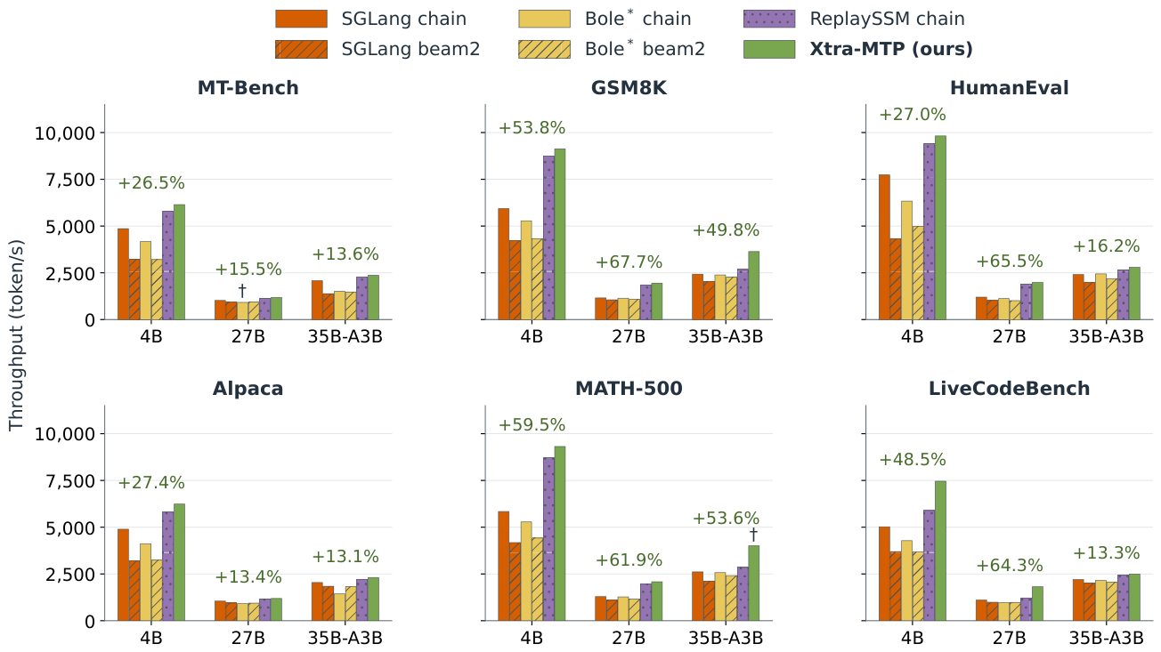
Figure A7.
Per-workload maximum measured throughput at request-TPOT p95 ms, using the same selection rule and encodings as Figure A6.
Figure A7.
Per-workload maximum measured throughput at request-TPOT p95 ms, using the same selection rule and encodings as Figure A6.
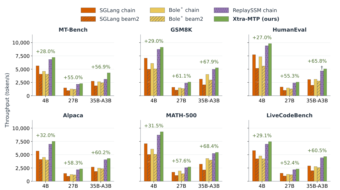
Table A3.
Maximum observed throughput at request-TPOT p95 ms (token/s/GPU), selecting D3/D7 and concurrency; Xtra also selects chain/H1. Gains use unrounded values and the better SGLang topology. †: p95 within 0.2 ms of the limit. Bole is our reproduction.
Table A3.
Maximum observed throughput at request-TPOT p95 ms (token/s/GPU), selecting D3/D7 and concurrency; Xtra also selects chain/H1. Gains use unrounded values and the better SGLang topology. †: p95 within 0.2 ms of the limit. Bole is our reproduction.
| Benchmark | SGLang | Bole | ReplaySSM chain |
Xtra-MTP (ours) |
Gain vs. SGLang |
Gain vs. best base. |
||
|---|---|---|---|---|---|---|---|---|
| chain | beam2 | chain | beam2 | |||||
| Qwen3.5-4B | ||||||||
| MT-Bench | 5636 | 3530 | 4175 | 3552 | 6810 | +28.0% | +5.9% | |
| Alpaca | 5691 | 3532 | 4119 | 3542 | 6975 | +32.0% | +7.7% | |
| GSM8K | 7073 | 4986 | 6087 | 5041 | 8738 | +29.0% | +4.4% | |
| MATH-500 | 7084 | 5041 | 6058 | 5094 | 8704 | +31.5% | +7.0% | |
| HumanEval | 7733 | 5166 | 7351 | 5593 | 9410 | +27.0% | +4.3% | |
| LiveCodeBench | 5779 | 3695 | 4281 | 3685 | 6970 | +29.1% | +7.0% | |
| Qwen3.8-27B-FP8 | ||||||||
| MT-Bench | 1475 | 950 | 926 | 936 | 1693 | +21.6% | +6.0% | |
| Alpaca | 1476 | 950 | 1268 | 1206 | 1705 | +20.7% | +4.5% | |
| GSM8K | 1597 | 1059 | 1483 | 1329 | 2385 | +61.1% | +7.9% | |
| MATH-500 | 1711 | 1094 | 1655 | 1414 | 2569 | +57.6% | +4.9% | |
| HumanEval | 1651 | 1019 | 1467 | 1287 | 2414 | +55.3% | +6.2% | |
| LiveCodeBench | 1514 | 988 | 1311 | 1235 | 1720 | +20.1% | +5.7% | |
| Qwen3.6-35B-A3B-FP8 | ||||||||
| MT-Bench | 2744 | 1874 | 2051 | 1941 | 3066 | +18.6% | +6.2% | |
| Alpaca | 2683 | 1841 | 1931 | 1870 | 3010 | +18.8% | +5.8% | |
| GSM8K | 3133 | 2041 | 3161 | 2963 | +67.9% | +5.7% | ||
| MATH-500 | 3231 | 2120 | 3373 | 3132 | 5242 | +68.4% | +3.8% | |
| HumanEval | 3048 | 1980 | 2509 | 3613 | +55.1% | +30.8% | ||
| LiveCodeBench | 2896 | 2002 | 2776 | 2486 | 3236 | +17.8% | +5.4% | |
Table A4.
Fixed D7/C64: k output tokens/s / request-TPOT p95 (ms), 1,920 requests per arm. Baselines use chain; both Xtra topologies are shown. Mem denotes a resource failure.
Table A4.
Fixed D7/C64: k output tokens/s / request-TPOT p95 (ms), 1,920 requests per arm. Baselines use chain; both Xtra topologies are shown. Mem denotes a resource failure.
| Task | SGLang | ReplaySSM | Bole | Xtra chain | Xtra H1 |
|---|---|---|---|---|---|
| Qwen3.5-4B | |||||
| MT-Bench | 4.00 / 24.8 | 4.85 / 20.3 | 4.00 / 24.3 | 5.16 / 18.6 | 4.94 / 19.0 |
| Alpaca | 3.98 / 22.9 | 4.86 / 18.7 | 3.93 / 23.0 | 5.21 / 17.3 | 4.99 / 18.1 |
| GSM8K | 5.34 / 14.9 | 6.40 / 12.5 | 5.28 / 14.8 | 6.78 / 11.6 | 6.45 / 12.0 |
| MATH-500 | 5.33 / 14.7 | 6.38 / 12.3 | 5.28 / 14.4 | 6.70 / 11.4 | 6.19 / 12.1 |
| HumanEval | 6.32 / 12.2 | 7.47 / 10.3 | 6.33 / 12.0 | 7.73 / 10.0 | 7.33 / 10.2 |
| LiveCodeBench | 4.24 / 18.6 | 5.07 / 15.5 | 4.13 / 18.7 | 5.40 / 14.5 | 4.92 / 15.4 |
| Qwen3.8-27B-FP8 | |||||
| MT-Bench | Mem | 1.80 / 50.7 | 1.43 / 64.3 | 1.95 / 46.2 | 1.81 / 50.6 |
| Alpaca | Mem | 1.76 / 47.7 | 1.39 / 58.0 | 1.90 / 42.1 | 1.77 / 46.4 |
| GSM8K | Mem | 2.18 / 34.1 | 1.74 / 43.0 | 2.35 / 31.5 | 2.16 / 33.8 |
| MATH-500 | Mem | 2.38 / 31.9 | 1.94 / 39.6 | 2.54 / 31.2 | 2.30 / 33.5 |
| HumanEval | Mem | 2.11 / 40.6 | 1.69 / 50.2 | 2.30 / 37.4 | 2.08 / 41.1 |
| LiveCodeBench | Mem | 1.85 / 44.2 | 1.49 / 55.2 | 1.95 / 41.9 | 1.79 / 44.1 |
| Qwen3.6-35B-A3B-FP8 | |||||
| MT-Bench | Mem | 3.10 / 31.2 | 2.64 / 35.5 | 3.26 / 29.7 | 3.22 / 28.5 |
| Alpaca | Mem | 2.92 / 28.5 | 2.47 / 33.8 | 3.13 / 27.4 | 3.04 / 27.9 |
| GSM8K | Mem | 3.63 / 21.2 | 3.16 / 23.7 | 3.75 / 20.3 | 3.68 / 20.2 |
| MATH-500 | Mem | 3.90 / 20.1 | 3.37 / 23.8 | 4.01 / 19.8 | 3.82 / 20.4 |
| HumanEval | Mem | 3.61 / 26.0 | 3.09 / 29.9 | 3.78 / 23.9 | 3.59 / 25.6 |
| LiveCodeBench | Mem | 3.24 / 24.3 | 2.78 / 28.1 | 3.40 / 23.0 | 3.08 / 24.7 |
Table A5.
Maximum observed throughput under lifetime process-memory budgets (token/s/GPU): geometric means of six task maxima, without a latency constraint. Gains use unrounded values and SGLang’s best supported configuration.
Table A5.
Maximum observed throughput under lifetime process-memory budgets (token/s/GPU): geometric means of six task maxima, without a latency constraint. Gains use unrounded values and SGLang’s best supported configuration.
| Budget (GiB) |
SGLang | Bole | ReplaySSM | Xtra-MTP (ours) |
Gain vs. SGLang |
Gain vs. best base. |
|---|---|---|---|---|---|---|
| Qwen3.5-4B | ||||||
| 16 | 2686 | 3739 | 4442 | +72.0% | +4.0% | |
| 24 | 4190 | 4922 | 6895 | +74.4% | +6.0% | |
| 32 | 5224 | 5470 | 7866 | +59.7% | +6.1% | |
| Qwen3.8-27B-FP8 | ||||||
| 40 | 421 | 1059 | 1255 | +209.3% | +3.8% | |
| 48 | 1045 | 1479 | 1956 | +99.1% | +6.4% | |
| 64 | 1568 | 1661 | 2302 | +56.6% | +6.7% | |
| Qwen3.6-35B-A3B-FP8 | ||||||
| 40 | 820 | 1650 | 1798 | +124.3% | +2.2% | |
| 48 | 1861 | 2902 | 3399 | +90.9% | +4.5% | |
| 64 | 2949 | 3654 | 4558 | +63.2% | +5.6% | |
Figure A8.
MT-Bench serving-stage process peak versus concurrency at D3/D7. NVML sampling interval is 50 ms; budgeted throughput instead uses lifetime peaks.
Figure A8.
MT-Bench serving-stage process peak versus concurrency at D3/D7. NVML sampling interval is 50 ms; budgeted throughput instead uses lifetime peaks.
Appendix C. GDN Implementation and Supporting Analysis
Appendix C.1. Residual Formulation and Kernel Execution
Expanding Equation 3 around the post-root checkpoint gives , where sums log-decays along i’s post-root path and is its normalized, scaled query. With denoting strict ancestry, residuals and outputs satisfy
The ancestor-ordered system has unit diagonal and a unique solution. In spine/leaf order,
terminal rows consume spine residuals without propagating to other rows.
Each Xtra program owns a request, value head and disjoint value tile. It recovers the selected suffix, absorbs the root, projects , solves residuals and reads out candidates. BF16x3 splits FP32 operands into BF16 high and residual parts, summing low–high, high–low and high–high matrix products with FP32 accumulation; the low–low product is omitted. State updates use FP32. Dense padded key products receive ancestry masks. The spine-first solve costs for padded extent and tile width , versus for the finite Neumann series , with p chosen so . Both keep intermediates on chip. These counts exclude projections, readout and recovery, which remain in lifecycle timing.
Serving adapters receive projected Q/K/V, gates, parents and physical state indices. ReplaySSM writes raw operands and folds the accepted prefix, including root, into FP32 checkpoints after selection. Bole uses normalized Q/K, masked log-decay differences and a value-tiled finite Neumann-series solve, followed by selected-state reconstruction; noncontiguous inputs are copied inside the timed path. Xtra defers that recovery to the next consumer.
Appendix C.2. State Recovery, Journal Reuse and Memory Accounting
The checkpoint plus selected raw suffix represents exactly the consumed prefix. Starting with an empty suffix, each round folds the old suffix, absorbs the guaranteed root, verifies candidates and records the selected cursor. These transitions establish the invariant by induction in real arithmetic. A bonus advances state when consumed as the next root. Recovery uses raw journal operands rather than transient solved residuals.
Private values can be overwritten after their owner’s last read. Shared keys, gates and cursor wait for all owners, then a same-stream kernel replaces them (Figure A9). Eager/Graph execution share one journal per physical pool. Prefill/decode, copy/export and release materialize pending paths; import, reuse and reset clear metadata. Convolution, KV selection and MTP refresh retain the same prefix.
Figure A9.
Journal ownership and overwrite order. Bar lengths show ordering, not measured duration.
Per layer, an FP32 checkpoint costs bytes; a raw record costs (BF16 keys/values, FP32 gates). For P slots and layers, Xtra stores conditional bytes plus metadata alongside the checkpoint, versus SGLang’s candidate bytes. Root absorption removes one record; aliasing is counted once. Recovering a selected records costs per head without intermediate matrix writes. The serving allocator retains a common conservative two-state reservation for compressed adapters; Table A6 counts actual allocations.
Table A6.
Memory at two distinct scopes. (a) Single-layer B16/D7, all values in MiB; workspace includes solve/readout buffers, and peak CUDA-allocator memory includes checkpoint/common inputs. (b) MT-Bench D7/C16, matched request/KV capacity; auxiliary excludes shared checkpoints, all state includes checkpoints and convolution, and process peaks cover measured serving.
Table A6.
Memory at two distinct scopes. (a) Single-layer B16/D7, all values in MiB; workspace includes solve/readout buffers, and peak CUDA-allocator memory includes checkpoint/common inputs. (b) MT-Bench D7/C16, matched request/KV capacity; auxiliary excludes shared checkpoints, all state includes checkpoints and convolution, and process peaks cover measured serving.
| Method | Vectors | Gates/meta. | Workspace | Auxiliary | CUDA peak | |
|---|---|---|---|---|---|---|
| 32 | Bole | 3.000 | 0.099 | 4.000 | 7.099 | 44.119 |
| 32 | ReplaySSM | 1.500 | 0.031 | 0.000 | 1.531 | 36.551 |
| 32 | Xtra | 1.312 | 0.028 | 0.000 | 1.340 | 36.361 |
| 48 | Bole | 4.000 | 0.130 | 5.500 | 9.630 | 64.158 |
| 48 | ReplaySSM | 2.000 | 0.047 | 0.000 | 2.047 | 54.074 |
| 48 | Xtra | 1.750 | 0.042 | 0.000 | 1.792 | 54.007 |
| Backend | 4B | 27B | 35B-A3B |
|---|---|---|---|
| SGLang | 6528.00 / 7.340 / 18.82 | 19584.00 / 21.936 / 55.11 | 8160.00 / 9.175 / 46.67 |
| ReplaySSM | 39.05 / 1.003 / 12.49 | 104.39 / 2.913 / 36.11 | 48.81 / 1.254 / 38.75 |
| Bole | 169.54 / 1.131 / 12.88 | 460.54 / 3.261 / 36.46 | 211.91 / 1.413 / 38.92 |
| Xtra chain | 34.17 / 0.998 / 12.49 | 91.34 / 2.900 / 36.08 | 42.71 / 1.248 / 38.75 |
| Xtra H1 | 39.05 / 1.022 / 13.73 | 104.39 / 2.959 / 37.32 | 48.81 / 1.277 / 40.09 |
At 4B/D7/C16, Xtra chain saves 12.5% of ReplaySSM’s records, with both process peaks at 12.49 GiB; H1 raises Xtra’s peak to 13.73 GiB.
Appendix C.3. Kernel Comparisons and Execution Controls
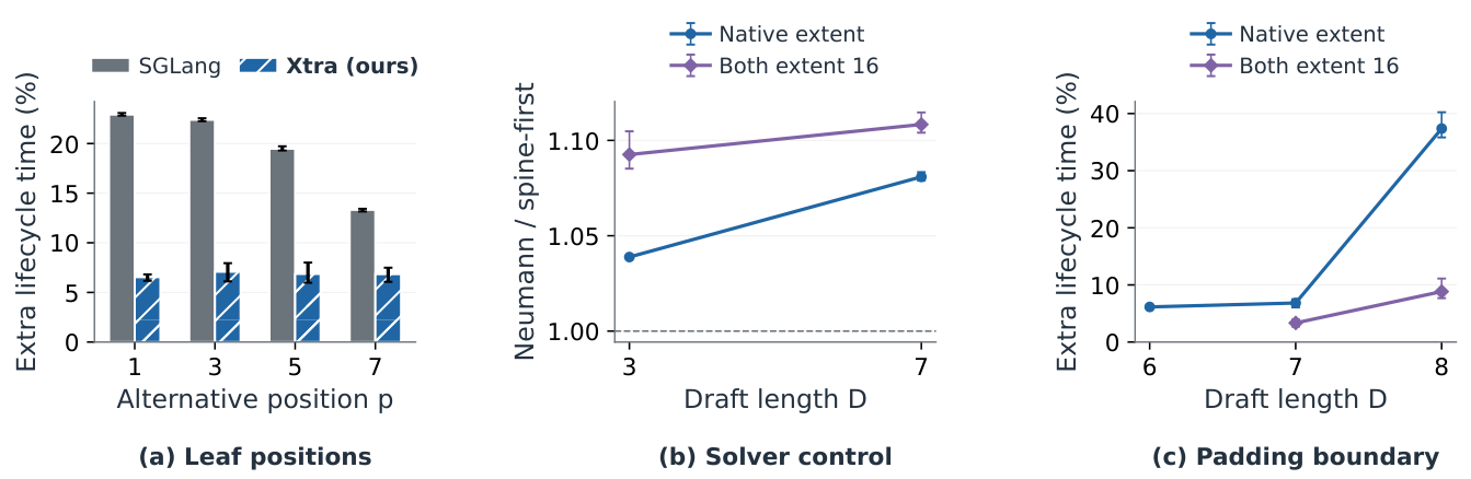
Figure A10 retains all batch/depth comparisons for both head geometries. Table A7 varies accepted length with raw-record representation and verifier tiling fixed: deferred recovery helps the mixed trace and every tested length at , while deferred recovery is 6.6% slower at . A separate two-layer root-record control saves records but increases latency by 9.8–17.0%; removing a record alone does not explain the final schedule’s speedup.
Figure A10.
Xtra GDN lifecycle speedup (baseline time / Xtra time); larger values favor Xtra. Two head geometries, three baselines, six batches and seven lengths; all include state maintenance and final materialization.
Figure A10.
Xtra GDN lifecycle speedup (baseline time / Xtra time); larger values favor Xtra. Two head geometries, three baselines, six batches and seven lengths; all include state maintenance and final materialization.
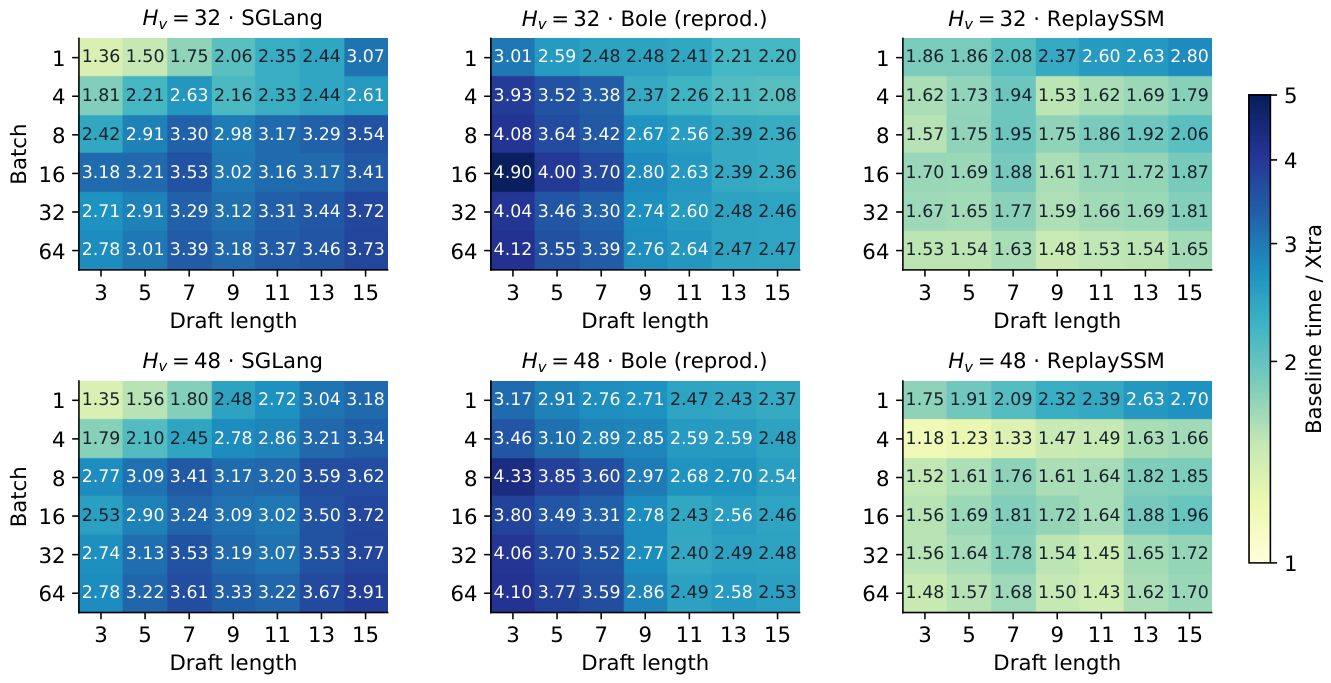
Table A7.
B16/D7 lifecycle time (s/round) versus committed drafts a. Mixed cycles and averages three processes; fixed lengths use one. Eager and Xtra share raw factors and tiling.
Table A7.
B16/D7 lifecycle time (s/round) versus committed drafts a. Mixed cycles and averages three processes; fixed lengths use one. Eager and Xtra share raw factors and tiling.
| a | ReplaySSM | Eager | Xtra | ReplaySSM | Eager | Xtra |
| Mixed | 118.36 | 65.51 | 63.14 | 189.37 | 138.87 | 104.80 |
| 0 | 101.12 | 50.57 | 47.89 | 166.95 | 97.90 | 84.19 |
| 1 | 107.22 | 64.02 | 52.83 | 171.92 | 146.36 | 89.03 |
| 3 | 119.48 | 67.36 | 63.63 | 190.30 | 149.02 | 103.74 |
| 5 | 132.05 | 74.25 | 74.44 | 210.01 | 156.83 | 119.73 |
| 7 | 144.05 | 81.09 | 86.45 | 229.77 | 166.66 | 137.66 |
Solver controls hold operands, BF16x3 projections, recovery and tiling fixed. Neumann products require reduction extent 16; the common-extent arm pads both residual systems to 16. The full-width control uses eight warps, matching four two-warp programs. At D8, natural chain/H1 extents 8/16 yield 37.4% late-leaf overhead; equal extent 16 reduces it to 8.8% (Figure A11). Tile shape contributes alongside dependency structure.
Figure A11.
B16/ controls; ranges span three paired processes. (a) D7 one-leaf overhead at four positions versus each backend’s chain. (b) Solver control with native/common extent 16. (c) Padding-boundary control with identical selected spine endpoints.
Figure A11.
B16/ controls; ranges span three paired processes. (a) D7 one-leaf overhead at four positions versus each backend’s chain. (b) Solver control with native/common extent 16. (c) Padding-boundary control with identical selected spine endpoints.
Appendix C.4. Candidate Topology and Complete-Model Costs
Appendix C.10.10.10. Coverage and placement.
The budget screen retains top-5 alternatives from a fixed spine. Root placement chooses the E highest root alternatives; global placement chooses the E largest reach-weighted scores over ranks 2–5, without a parent-count cap. The deployed rule uses . Projection work in Table A8 counts MTP/target rows at 1.51257088/8.40957952 GFLOPs each, including block, MLP, vocabulary and MTP-fusion projections. It excludes shared MTP initialization/refresh, attention, state updates, sampling and padding.
Table A8.
Matched 4B/D7 first-prefix coverage and projection work. is chain; accepted drafts exclude root/bonus, verify nodes include root. The final column divides Global’s accepted-length increment by beam2’s.
Table A8.
Matched 4B/D7 first-prefix coverage and projection work. is chain; accepted drafts exclude root/bonus, verify nodes include root. The final column divides Global’s accepted-length increment by beam2’s.
| E | Root | Global | MTP rows | Verify nodes | GFLOPs | Gain / beam (%) |
|---|---|---|---|---|---|---|
| 0 | 4.777 | 4.777 | 6 | 8 | 76.35 | 0.0 |
| 1 | 4.814 | 4.950 | 6 | 9 | 84.76 | 25.6 |
| 2 | 4.825 | 5.044 | 6 | 10 | 93.17 | 39.6 |
| 4 | 4.825 | 5.118 | 6 | 12 | 109.99 | 50.4 |
| beam2 | 5.452 | 5.452 | 12 | 15 | 144.29 | 100.0 |
On these 191 prefixes, zero acceptance is 5.26/1.58/3.16/2.11% for chain/root/global/beam2: root placement best suppresses immediate rejection, while global placement recovers more mean progress. The separate 27B/D7 position diagnostic pools 1,286 rounds from 48 requests (384 full-depth); 251 of 308 possible top-2 rescues occur after position one. Both position bars use all rounds as denominator.
Table A9.
Placement controls: (a) common-prefix acceptance, 48 requests/row; (b) matched-profile serving, 192 requests/arm, with shared controller, Graph and capacity for root/global. Zero denotes .
Table A9.
Placement controls: (a) common-prefix acceptance, 48 requests/row; (b) matched-profile serving, 192 requests/arm, with shared controller, Graph and capacity for root/global. Zero denotes .
| Model / D | Chain | Root H1 | Global H1 |
|---|---|---|---|
| (a) Common-prefix acceptance: / zero (%) / (%) | |||
| 4B / 3 | 2.512 / 7.16 / 17.12 | 2.545 / 3.87 / 17.12 | 2.597 / 4.16 / 13.92 |
| 4B / 7 | 4.832 / 7.50 / 18.65 | 4.868 / 3.95 / 18.65 | 4.965 / 4.47 / 15.43 |
| 27B / 3 | 2.400 / 9.38 / 16.20 | 2.440 / 5.36 / 16.20 | 2.488 / 5.85 / 13.30 |
| 27B / 7 | 4.354 / 9.36 / 17.06 | 4.389 / 5.89 / 17.06 | 4.479 / 7.27 / 15.27 |
| 35B-A3B / 3 | 2.286 / 13.09 / 24.09 | 2.324 / 9.27 / 24.09 | 2.370 / 10.01 / 21.12 |
| 35B-A3B / 7 | 4.083 / 15.84 / 26.93 | 4.131 / 11.06 / 26.93 | 4.217 / 12.13 / 24.86 |
| (b) D7/C16 matched-profile serving: token/s / p95 (ms) | |||
| 4B | 3615 / 6.14 | 3506 / 6.01 | 3558 / 5.67 |
| 27B | 1230 / 17.71 | 1113 / 19.70 | 1154 / 19.30 |
| 35B-A3B | 1787 / 11.67 | 1644 / 12.66 | 1689 / 12.30 |
Appendix C.10.10.11. Request-TPOT distributions.
Figure A12 divides each method’s TPOT by its own median. Table A10 pairs absolute latency and throughput with , the relative upper tail. H1 lowers both p95 and versus Xtra chain in these D3/C4 runs. On 27B, p50/p95 fall together (9.145/11.439 to 8.742/10.751 ms); the change is smaller, 1.251 to 1.230. On 35B, beam2 lowers SGLang’s from 1.321 to 1.196 while raising both p50 and p95. A narrower relative tail can therefore coexist with higher absolute latency.
Figure A12.
Median-normalized request-TPOT CDFs for the same MT-Bench D3/ runs as Figure 3. Each method uses its own median. Horizontal/vertical guides mark 95% of requests and the median.
Figure A12.
Median-normalized request-TPOT CDFs for the same MT-Bench D3/ runs as Figure 3. Each method uses its own median. Horizontal/vertical guides mark 95% of requests and the median.
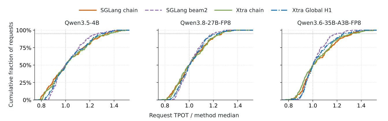
Table A10.
MT-Bench D3/: measured throughput and request-TPOT quantiles, 160 requests per arm. . Models are the three checkpoints in Section 5.1; all values come from the same runs as Figure 3.
Table A10.
MT-Bench D3/: measured throughput and request-TPOT quantiles, 160 requests per arm. . Models are the three checkpoints in Section 5.1; all values come from the same runs as Figure 3.
| Model | Configuration | token/s | p50 (ms) | p95 (ms) | |
|---|---|---|---|---|---|
| 4B | SGLang chain | 963 | 3.907 | 5.187 | 1.328 |
| SGLang beam2 | 944 | 4.003 | 5.040 | 1.259 | |
| Xtra chain | 1,034 | 3.619 | 4.916 | 1.358 | |
| Xtra Global H1 | 1,037 | 3.615 | 4.680 | 1.295 | |
| 27B | SGLang chain | 395 | 9.618 | 12.175 | 1.266 |
| SGLang beam2 | 398 | 9.516 | 11.351 | 1.193 | |
| Xtra chain | 416 | 9.145 | 11.439 | 1.251 | |
| Xtra Global H1 | 433 | 8.742 | 10.751 | 1.230 | |
| 35B-A3B | SGLang chain | 784 | 4.669 | 6.167 | 1.321 |
| SGLang beam2 | 708 | 5.338 | 6.385 | 1.196 | |
| Xtra chain | 807 | 4.568 | 5.977 | 1.308 | |
| Xtra Global H1 | 790 | 4.687 | 5.873 | 1.253 |
Appendix C.10.10.12. Concurrency and full-model costs.
At D3/ on the same workload, H1 raises p95 by 2.0/0.3/1.7% and reduces throughput by 2.3/1.5/3.7% for 4B/27B/35B-A3B. Across all 276 paired H1/chain configurations, 108 have lower p95, 197 lower , and 89 improve both. These per-run observations motivate profiling candidate budgets for the intended operating point.
In the separate D7/ matched-profile controls (Table A9b), global placement improves throughput over root by 1.5/3.6/2.8%, while chain remains faster in all three models; Global improves chain p95 on 4B. At D7/, MT-Bench H1 increases progress per request-verification by 5.3–7.6% while reducing throughput by 1.2–7.2%; the 27B changes are +6.6% and . Full-model profiles retain substantial MTP and non-GDN costs (Figure A13).
Figure A13.
Complete-model diagnostics. (a) GPU phase sums over three warmed H1 rounds, D7/C16; S/X are SGLang/Xtra with independently generated prefixes. (b) Xtra H1 versus chain progress/throughput on MT-Bench D7/C64.
Figure A13.
Complete-model diagnostics. (a) GPU phase sums over three warmed H1 rounds, D7/C16; S/X are SGLang/Xtra with independently generated prefixes. (b) Xtra H1 versus chain progress/throughput on MT-Bench D7/C64.
Appendix C.5. Numerical Validation
The state representation preserves the original recurrence in real arithmetic. Block projections and solving reorder floating-point operations, introducing rounding and accumulation error. We measure these errors on seven chain/tree shapes per GDN geometry over 48 feedback rounds, varying parents, accepted leaves, padding and slot permutations without flushing live journals for checks. Maximum output relative error is ; logical-state relative error is . Pool checks cover copy, export/import, prefill, release and reuse.
Execution controls separately use eleven B2/ shapes and eight feedback rounds. Against SGLang, maximum output absolute/relative errors are ; state absolute/relative errors are . All pass the fixed output gates and state gates . The isolated spine-first implementation also matches the released Xtra outputs/exported states bytewise.
References
- DeepSeek-AI. 2026. DeepSeek-V4: Towards Highly Efficient Million-Token Context Intelligence. arXiv arXiv:2606.19348. [Google Scholar]
- Qwen Team. 2026. Qwen3.5: Towards Native Multimodal Agents. [Google Scholar] [CrossRef]
- Leviathan, Y., M. Kalman, and Y. Matias. 2023. Fast Inference from Transformers via Speculative Decoding. Proceedings of the Proceedings of the 40th International Conference on Machine Learning; p. 2211.17192. [Google Scholar]
- Agrawal, A., N. Kedia, A. Panwar, J. Mohan, N. Kwatra, B. Gulavani, A. Tumanov, and R. Ramjee. 2024. Taming Throughput-Latency Tradeoff in LLM Inference with Sarathi-Serve. Proceedings of the 18th USENIX Symposium on Operating Systems Design and Implementation (OSDI 24); pp. 117–134. [Google Scholar]
- Sadhukhan, R., J. Chen, Z. Chen, V. Tiwari, R. Lai, J. Shi, I.E.H. Yen, A. May, T. Chen, and B. Chen. 2025. MagicDec: Breaking the Latency-Throughput Tradeoff for Long Context Generation with Speculative Decoding. Proceedings of the International Conference on Learning Representations. [Google Scholar]
- Dao, AI Lab. 2026. ReplaySSM: Cache SSM Inputs, Not State. Technical blog. (accessed on 2026-09-03).
- Wang, L., Y. Su, X. Wu, C. You, Y. Liu, Z. Qiu, J. Zhang, J. Zheng, F. Liu, J. Zhang, and et al. 2026. Bole: Efficient Tree Speculation for Hybrid-Attention Language Models. arXiv arXiv:2608.01651. [Google Scholar]
- Yang, S., J. Kautz, and A. Hatamizadeh. 2025. Gated Delta Networks: Improving Mamba2 with Delta Rule. Proceedings of the International Conference on Learning Representations; p. 2412.06464. [Google Scholar]
- Zheng, L., L. Yin, Z. Xie, C. Sun, J. Huang, C.H. Yu, S. Cao, C. Kozyrakis, I. Stoica, J.E. Gonzalez, and et al. 2024. SGLang: Efficient Execution of Structured Language Model Programs. Proceedings of the Advances in Neural Information Processing Systems Vol. 37. [Google Scholar] [CrossRef]
- Qwen Team. 2026. Qwen3.8-Max: A New Bar for Coding and Cowork. [Google Scholar] [PubMed]
- Qwen Team. 2026. Qwen3.6-35B-A3B: Agentic Coding Power, Now Open to All. [Google Scholar] [PubMed]
- Zheng, L., W.L. Chiang, Y. Sheng, S. Zhuang, Z. Wu, Y. Zhuang, Z. Lin, Z. Li, D. Li, E.P. Xing, and et al. 2023. Judging LLM-as-a-judge with MT-Bench and Chatbot Arena. Proceedings of the Advances in Neural Information Processing Systems Vol. 36. [Google Scholar] [CrossRef]
- Taori, R., I. Gulrajani, T. Zhang, Y. Dubois, X. Li, C. Guestrin, P. Liang, and T.B. Hashimoto. 2023. Stanford Alpaca: An Instruction-following LLaMA Model. Stanford CRFM project. [Google Scholar]
- Cobbe, K., V. Kosaraju, M. Bavarian, M. Chen, H. Jun, L. Kaiser, M. Plappert, J. Tworek, J. Hilton, R. Nakano, and et al. 2021. Training Verifiers to Solve Math Word Problems. arXiv arXiv:2110.14168. [Google Scholar]
- Lightman, H., V. Kosaraju, Y. Burda, H. Edwards, B. Baker, T. Lee, J. Leike, J. Schulman, I. Sutskever, and K. Cobbe. 2023. Let’s Verify Step by Step. arXiv arXiv:2305.20050. [Google Scholar]
- Hendrycks, D., C. Burns, S. Kadavath, A. Arora, S. Basart, E. Tang, D. Song, and J. Steinhardt. 2021. Measuring Mathematical Problem Solving With the MATH Dataset. NeurIPS. [Google Scholar] [CrossRef]
- Chen, M., J. Tworek, H. Jun, Q. Yuan, H.P. de Oliveira Pinto, J. Kaplan, H. Edwards, Y. Burda, N. Joseph, G. Brockman, and et al. 2021. Evaluating Large Language Models Trained on Code. arXiv arXiv:2107.03374. [Google Scholar]
- Jain, N., K. Han, A. Gu, W.D. Li, F. Yan, T. Zhang, S. Wang, A. Solar-Lezama, K. Sen, and I. Stoica. 2024. LiveCodeBench: Holistic and Contamination Free Evaluation of Large Language Models for Code. arXiv arXiv:2403.07974. [Google Scholar]
- Chen, C., S. Borgeaud, G. Irving, J.B. Lespiau, L. Sifre, and J. Jumper. 2023. Accelerating Large Language Model Decoding with Speculative Sampling. arXiv arXiv:2302.01318. [Google Scholar]
- Miao, X., G. Oliaro, Z. Zhang, X. Cheng, Z. Wang, Z. Zhang, R.Y.Y. Wong, A. Zhu, L. Yang, X. Shi, and et al. 2024. SpecInfer: Accelerating Large Language Model Serving with Tree-based Speculative Inference and Verification. Proceedings of the Proceedings of the 29th ACM International Conference on Architectural Support for Programming Languages and Operating Systems, Volume 3; ACM, pp. 932–949. [Google Scholar] [CrossRef]
- Cai, T., Y. Li, Z. Geng, H. Peng, J.D. Lee, D. Chen, and T. Dao. 2024. Medusa: Simple LLM Inference Acceleration Framework with Multiple Decoding Heads. Proceedings of the Proceedings of the 41st International Conference on Machine Learning. PMLR Vol. 235: 5209–5235. [Google Scholar]
- Li, Y., F. Wei, C. Zhang, and H. Zhang. 2024. EAGLE: Speculative Sampling Requires Rethinking Feature Uncertainty. Proceedings of the Proceedings of the 41st International Conference on Machine Learning. PMLR Vol. 235: 28935–28948. [Google Scholar]
- Li, Y., F. Wei, C. Zhang, and H. Zhang. 2025. EAGLE-3: Scaling up Inference Acceleration of Large Language Models via Training-Time Test. Proceedings of the Advances in Neural Information Processing Systems Vol. 38. [Google Scholar] [CrossRef]
- Chen, J., Y. Liang, and Z. Liu. 2026. DFlash: Block Diffusion for Flash Speculative Decoding. arXiv arXiv:2602.06036. [Google Scholar]
- Hu, L., Z. Feng, Y. Wu, H. Yuan, Y. Zhao, Y.Y. Qian, B. Wang, P. Zhao, D. Jiang, Y. Zhu, and et al. 2026. JetSpec: Breaking the Scaling Ceiling of Speculative Decoding with Parallel Tree Drafting. arXiv arXiv:2606.18394. [Google Scholar]
- Li, Y., F. Wei, C. Zhang, and H. Zhang. 2024. EAGLE-2: Faster Inference of Language Models with Dynamic Draft Trees. Proceedings of the Proceedings of the 2024 Conference on Empirical Methods in Natural Language Processing; Association for Computational Linguistics, pp. 7421–7432. [Google Scholar] [CrossRef]
- Chen, Z., A. May, R. Svirschevski, Y. Huang, M. Ryabinin, Z. Jia, and B. Chen. 2024. Sequoia: Scalable, Robust, and Hardware-aware Speculative Decoding. arXiv arXiv:2402.12374. [Google Scholar]
- Gloeckle, F., B. Youbi Idrissi, B. Rozière, D. Lopez-Paz, and G. Synnaeve. 2024. Better & Faster Large Language Models via Multi-token Prediction. Proceedings of the Proceedings of the 41st International Conference on Machine Learning. PMLR Vol. 235: 15706–15734. [Google Scholar]
- Wu, Y., Y. Dukler, M. Trager, A. Achille, W. Xia, and S. Soatto. 2024. Snakes and Ladders: Accelerating SSM Inference with Speculative Decoding. Proceedings of the Proceedings of the 4th NeurIPS Efficient Natural Language and Speech Processing Workshop. PMLR Vol. 262: 292–304. [Google Scholar]
- Borobia, H., E. Seguí-Mas, and G. Tormo-Carbó. 2026. Component-Aware Self-Speculative Decoding in Hybrid Language Models. arXiv arXiv:2605.01106. [Google Scholar]
- Ghantasala, S.M. 2026. TreeWY: Speculative Verification for Gated DeltaNet Hybrids. arXiv arXiv:2608.20961. [Google Scholar]
- Zhong, Y., S. Liu, J. Chen, J. Hu, Y. Zhu, X. Liu, X. Jin, and H. Zhang. 2024. DistServe: Disaggregating Prefill and Decoding for Goodput-Optimized Large Language Model Serving. Proceedings of the 18th USENIX Symposium on Operating Systems Design and Implementation (OSDI 24); pp. 193–210. [Google Scholar]
- Huang, K., H. Wu, Z. Shi, H. Zou, M. Yu, and Q. Shi. 2025. AdaSpec: Adaptive Speculative Decoding for Fast, SLO-Aware Large Language Model Serving. Proceedings of the Proceedings of the 2025 ACM Symposium on Cloud Computing. [Google Scholar] [CrossRef]
Figure 1.
Three verification bottlenecks. (a) Native MTP D7 request-TPOT p50/p95/p99 reductions versus autoregressive (AR) decoding, Qwen3.8-27B-FP8, , 512 output tokens; negative means slower MTP. (b) Qwen3.5-4B candidate GDN storage versus weights plus 128K-token target/MTP KV pools, . (c) Target-only speedup, , prefix 256; *: Instruct-2507, †: cross-GPU decode bracket. D excludes root; protocols are in Appendix A.2.
Figure 1.
Three verification bottlenecks. (a) Native MTP D7 request-TPOT p50/p95/p99 reductions versus autoregressive (AR) decoding, Qwen3.8-27B-FP8, , 512 output tokens; negative means slower MTP. (b) Qwen3.5-4B candidate GDN storage versus weights plus 128K-token target/MTP KV pools, . (c) Target-only speedup, , prefix 256; *: Instruct-2507, †: cross-GPU decode bracket. D excludes root; protocols are in Appendix A.2.
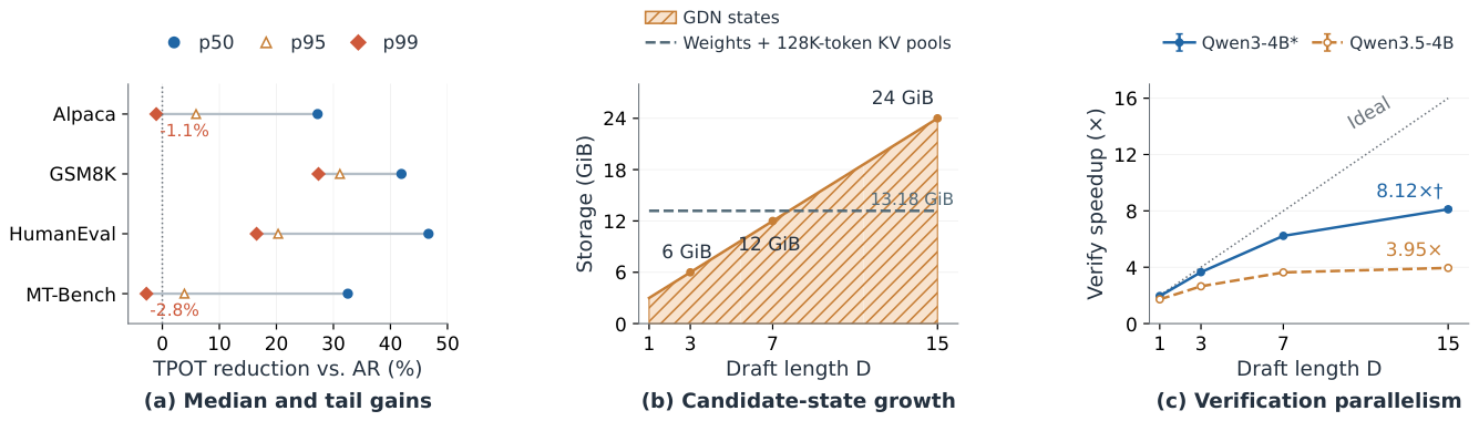
Figure 2.
(a) First mismatches and potential top-2 rescues, all 1,286 27B/D7 rounds. (b) Root/Global H1, : projection FLOPs versus mean accepted drafts, 191 matched 4B/D7 prefixes, equal task weights. (c) 4B/GSM8K/D7 throughput relative to each backend’s chain. D: spine length; H: side-branch length; E: extra leaves.
Figure 2.
(a) First mismatches and potential top-2 rescues, all 1,286 27B/D7 rounds. (b) Root/Global H1, : projection FLOPs versus mean accepted drafts, 191 matched 4B/D7 prefixes, equal task weights. (c) 4B/GSM8K/D7 throughput relative to each backend’s chain. D: spine length; H: side-branch length; E: extra leaves.
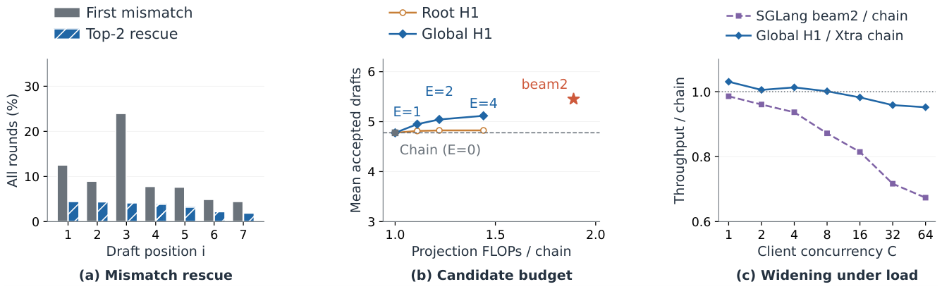
Figure 3.
Request-average TPOT cumulative distribution functions (CDFs) on MT-Bench, D3/: 160 requests per method, each generating 512 tokens. The horizontal guide marks 95% of requests. Median-normalized distributions and numerical summaries appear in Appendix C.10.10.11.
Figure 3.
Request-average TPOT cumulative distribution functions (CDFs) on MT-Bench, D3/: 160 requests per method, each generating 512 tokens. The horizontal guide marks 95% of requests. Median-normalized distributions and numerical summaries appear in Appendix C.10.10.11.
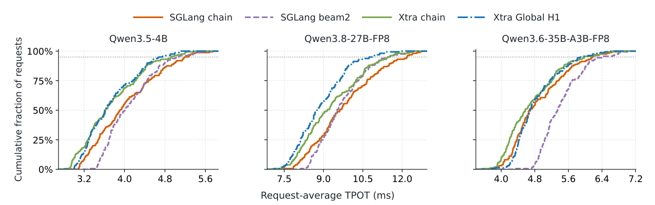
Figure 4.
GDN state and execution controls, . (a) Peak CUDA-allocator memory; solid/dashed: . (b) Profiled time at B16/D7, selected drafts ; forward includes fused recovery. (c) B16 chain lifecycle. (d) Solver/value-width changes within Xtra, D7. (c–d) use ; whiskers span three paired processes. All lifecycle timings include final materialization. Bole is our reproduction.
Figure 4.
GDN state and execution controls, . (a) Peak CUDA-allocator memory; solid/dashed: . (b) Profiled time at B16/D7, selected drafts ; forward includes fused recovery. (c) B16 chain lifecycle. (d) Solver/value-width changes within Xtra, D7. (c–d) use ; whiskers span three paired processes. All lifecycle timings include final materialization. Bole is our reproduction.
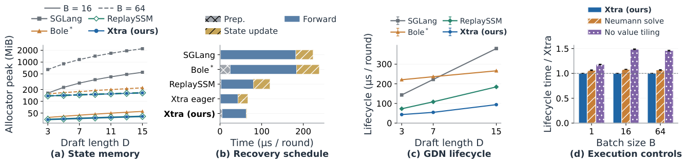
Figure 5.
Output and continuation paths, . Target selection retains suffix ; the bonus becomes the next root. The next value-tile owner folds the suffix and root before checkpoint projection, solve and readout. The selected cursor fixes the logical continuation before its full matrix is materialized; raw records come from upstream QKV/gate projections.
Figure 5.
Output and continuation paths, . Target selection retains suffix ; the bonus becomes the next root. The next value-tile owner folds the suffix and root before checkpoint projection, solve and readout. The selected cursor fixes the logical continuation before its full matrix is materialized; raw records come from upstream QKV/gate projections.
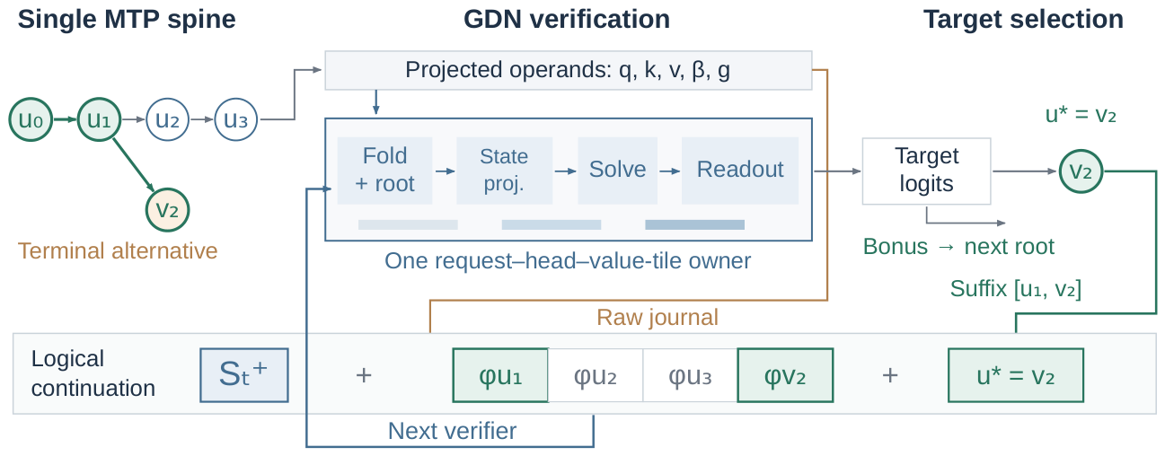
Figure 6.
Throughput–latency trade-offs across six workloads. Xtra selects chain/H1 at each profiled operating point. Points retain paired measurements from complete runs; lines are task-balanced Gaussian-kernel regression fits. Vertical guides compare throughput at matched request-p95 TPOT; horizontal guides compare p95 at matched throughput. Annotations give fitted maxima over the domains in Appendix A.3. Bole is our reproduction.
Figure 6.
Throughput–latency trade-offs across six workloads. Xtra selects chain/H1 at each profiled operating point. Points retain paired measurements from complete runs; lines are task-balanced Gaussian-kernel regression fits. Vertical guides compare throughput at matched request-p95 TPOT; horizontal guides compare p95 at matched throughput. Annotations give fitted maxima over the domains in Appendix A.3. Bole is our reproduction.
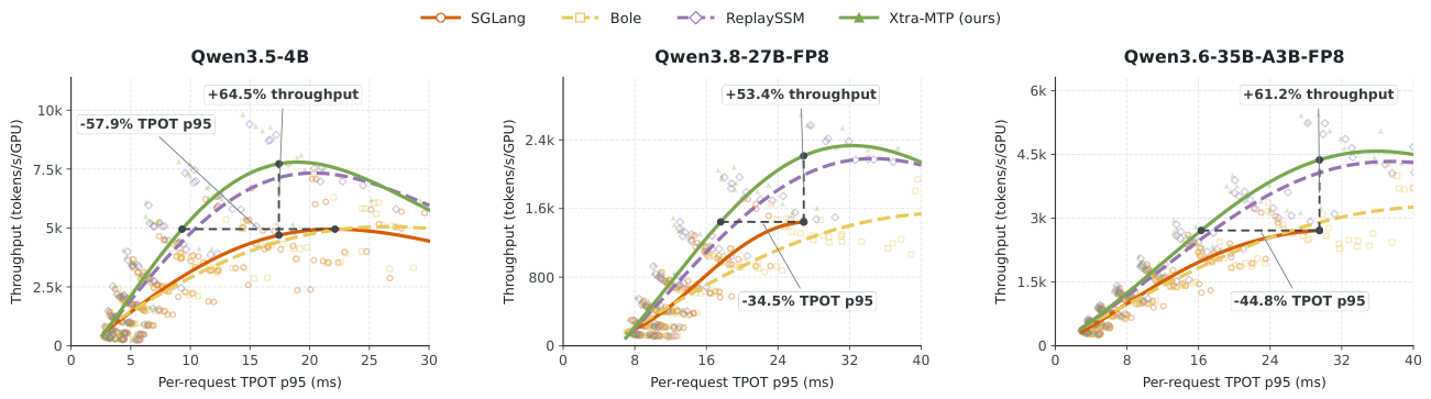
Figure 7.
Maximum measured throughput per GPU under a 30 ms request-p95 TPOT budget. Each bar uses the best measured D3/D7 and concurrency configuration; Xtra also selects chain/H1. Percentages show Xtra’s gains over the faster of SGLang chain and beam2. Bole denotes our reproduction.
Figure 7.
Maximum measured throughput per GPU under a 30 ms request-p95 TPOT budget. Each bar uses the best measured D3/D7 and concurrency configuration; Xtra also selects chain/H1. Percentages show Xtra’s gains over the faster of SGLang chain and beam2. Bole denotes our reproduction.
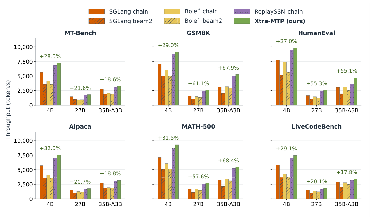
Figure 8.
Six-workload throughput under sampled process-memory budgets. Steps mark better feasible measured configurations; all six tasks must be covered. Markers identify budgets tabulated in Table A5. Panels use separate axis ranges.
Figure 8.
Six-workload throughput under sampled process-memory budgets. Steps mark better feasible measured configurations; all six tasks must be covered. Markers identify budgets tabulated in Table A5. Panels use separate axis ranges.
Disclaimer/Publisher’s Note: The statements, opinions and data contained in all publications are solely those of the individual author(s) and contributor(s) and not of MDPI and/or the editor(s). MDPI and/or the editor(s) disclaim responsibility for any injury to people or property resulting from any ideas, methods, instructions or products referred to in the content. |
© 2026 by the authors. Licensee MDPI, Basel, Switzerland. This article is an open access article distributed under the terms and conditions of the Creative Commons Attribution (CC BY) license (http://creativecommons.org/licenses/by/4.0/).
Copyright: This open access article is published under a Creative Commons CC BY 4.0 license, which permit the free download, distribution, and reuse, provided that the author and preprint are cited in any reuse.